Article

Demand-Driven Resilient Control for Generation Unit of Local Power Plant Under Unreliable Communication

1
State Grid Henan Electric Power Research Institute, Zhengzhou 450052, China
2
Henan Electric Power Dispatching and Control Center, Zhengzhou 450001, China
3
Shangqiu Power Supply Company, State Grid Henan Electric Power Company, Shangqiu 476002, China
4
School of Electrical and Information Engineering, Zhengzhou University, Zhengzhou 450001, China
*
Author to whom correspondence should be addressed.
Energies 2025, 18(2), 300; https://doi.org/10.3390/en18020300
Submission received: 8 December 2024 / Revised: 8 January 2025 / Accepted: 8 January 2025 / Published: 11 January 2025

Abstract

:
The resilient control issue for the generation unit (GU) in a local power plant with unreliable communication is addressed in this article, where the communication may be jammed by denial-of-service (DoS) attacks. Based on the GU model of voltage and current at the point of common coupling, a demand-driven network communication protocol is proposed to decrease the number of scheduling signal transmissions, and an observer-based prediction method is provided to replenish the lack of dispatching data during transmission intervals when the demand has not changed. The closed-loop performance is analyzed for the GU system in the input-to-state stable framework with or without attack. According to the DoS attack model, which is described by the assumptions of frequency and duration, the conservativeness of the tolerable DoS attack index is reduced by using the thought of robustness to the maximum disturbance-induced error. Simulation examples are provided to verify the effectiveness of the approach proposed in this article.

1. Introduction

In recent decades, with the vigorous progress of renewable energy, the randomness of renewable generation such as wind power and photovoltaics has made the smooth scheduling of power systems a hot topic [1]. In order to enhance the flexible capacity and peaking capacity of the power system, voltage and frequency control of small generation units (GUs) in local power plants becomes necessary. Recently, the scheduling scheme based on network communication has been widely used in power systems [2]. However, the utilization of heterogeneous electrical and electronic components with networks has made the data transmission fairly open to various cyber attacks. This can lead to serious security consequences. Unlike the attacks on traditional systems that limit the influence to the cyber level, the physical world of power systems can be impacted by malicious cyber attacks [3], causing serious social and livelihood problems. Thus, these strong demands for power systems exist, despite malicious cyber attacks, designing analysis and synthesis approaches to ensure their reliability and security [4,5].
Typically, the various malicious attacks involve deception attacks and denial-of-service (DoS) attacks, where the latter attack leads to the information absence of the actuator and sensor by blocking the data transmission to their respective destinations. The DoS attack is very common in networked control systems, and lots of studies have been presented on networked power systems under DoS attacks. In [6], an H load frequency control based on an event-triggered strategy is studied for multi-area power systems, and the resilient control approach is proposed to deal with the presence of DoS attacks. Security issues in remote state estimation with the existence of jamming attacks are investigated in [7] using a game-theoretic approach. In [8,9], the optimal DoS attack strategies for maximizing the deterioration on the system performance from the view of the adversary are investigated.
Stability analysis is a popular research topic on security problems of control systems under DoS attacks. In [10], the DoS attack model is characterized according to its frequency and duration, input-to-state stable (ISS) is demonstrated for the attacked closed-loop system, and transmission timing is scheduled based on this DoS attack model. Based on the analysis strategy proposed in [10], to maximize the attack intensity index according to the frequency and duration of the attack model with which the stability of the system is not destroyed, a resilient control framework is proposed in [11]. In [12], the controller design and analysis is investigated with this DoS attack model for nonlinear dynamics. In [13], based on the ISS control framework, the scenario of multiple transmission channels is considered for linear systems under DoS attacks. In [14], an output-based synthetical control design strategy for a class of hybrid nonlinear dynamics under DoS attacks is provided in a dynamic event-triggered framework. In [15], observer-based asynchronous control for switching power systems subject to DoS attacks is discussed. However, research on the resilient control of power systems under the condition of unreliable communication is still insufficient; particularly, the design of the output voltage and current control scheme of the GU via the network is still a challenging problem.
Traditionally, the control algorithms are executed in the time-scheduled strategy, in which the sampling and data communication are carried out periodically. Although the time-based periodic sampling might be preferable from the point of view of system analysis and design, it leads to the unnecessary waste of limited resources. Usually, network-based scheduling signals in power systems are not transmitted in real time but communicate when scheduling needs arise. In this way, the traditional time-triggered control method is no longer suitable. The event-triggered control scheme as a control strategy based on intermittent communication has been a wide concern for networked control systems [16,17,18], and it can be used to construct a demand-based control scheme for GUs. In [19], an event-triggered control (ETC) strategy with a periodic verification mechanism for linear systems is proposed, which is named periodic event-triggered control (PETC). By merging the time-scheduled strategy and ETC, the characteristic of PETC is to verify the triggering condition periodically—that is, whether to calculate and send new sampling data or new control data is determined at each periodic verification time. In [20], consider the scenario where both the sensor-to-controller channel and the controller-to-actuator channel are communicated via a network, a PETC algorithm is designed according to the retrievable system state space model. The above studies are all about networked control systems without attacks. Practically, power system scheduling also has a fixed sampling period; however, it is still a challenge to construct a resilient control scheme for the GU under unreliable communication using the idea of PETC.
For grid-connected power plants, the purpose of scheduling is to maintain the balance and stability of voltage and frequency, which are specified by the main grid when there are demands. However, for the local power plants tasked with flexibility and peaking, voltage and frequency outputs for GU are definitively controlled according to the networked scheduling signals, and it is necessary to save network resources. By introducing the concept of neutral interactions, the dynamic model of GU in this paper is established by exploiting quasi-stationary line approximations of line dynamics [21]. To improve the security of networked scheduling, the unreliable network communication channel is modeled as the communication interruption of the sensor channel due to the presence of a DoS attack. To construct the control framework, a smart sensor system is adopted in order to design the demand-driven mechanism (DDM)—that is, network communication is performed only when scheduling is required. Unfortunately, in the design of the control system, the load current of the unit connection is difficult to estimate. The conventional idea is to treat it as an unknown disturbance, but how to deal with the error term introduced by disturbance and noise is still a difficult point in the DDM design. To improve resilience against DoS attacks, a predictor is proposed in the controller system to compensate for the lack of data during communication intervals. Based on the ISS analysis framework, the stability when there are DoS attacks is proved and the maximum tolerable attack intensity index is quantified.
The prime innovations of this article are generalized below: First, the dynamic model of the GU for local power plant is established by exploiting quasi-stationary line approximations, and the unknown loads are treated as unmodeled disturbances, which can be restricted by the designed H observer. At the same time, the effects of disturbance and noise during the DDM design can be addressed by the quantified H performance index. Second, the advanced demand-driven resilient control method with a periodic verification strategy is presented to deal with the unreliable communication caused by DoS attacks, and the intermittent communication scenario meets the requirements of network scheduling for the GU by applying the prediction-based method. Third, based on the thought of robustness to the maximum disturbance accumulation error, the conservatism of the tolerable attack intensity in this result is decreased compared with [10,14].
The rest of this article is organized as follows: The GU model is described in Section 2, and the observer and the predictor are designed. In Section 3, the ISS of the demand-driven control approach is proved. Section 4 gives the resilient control strategy under DoS attacks. Section 5 provides simulation results. The conclusions of this paper are given in Section 6.

2. System Formulation and Problem Description

First of all, the meanings of the symbols used in this paper are shown in the notation below. Then, the state space model of the GU is constructed, and the resilient control framework is designed based on it.
Notation: Let R and R n be the sets of real and Euclidean spaces with dimension n, respectively. Let N be the natural number set and N 0 = N 0 . x denotes the Euclidean norm for any vector x R n . A T is the transpose of a given matrix A, A is the spectral norm, and μ A is the logarithmic norm [22] with μ A = max λ | λ spectrum A + A T 2 . For sets S 1 and S 2 , denote S 2 S 1 by the relative complement of S 1 in S 2 . T ( t 1 , t 2 ) = t 2 t 1 denotes by the length of an interval T = [ t 1 , t 2 ) . For a measurable function h ( t ) defined in [ 0 , t ) , the L norm of h ( · ) is denoted by h t = e s s sup s [ 0 , t ) h ( s ) .

2.1. Generation Unit Model

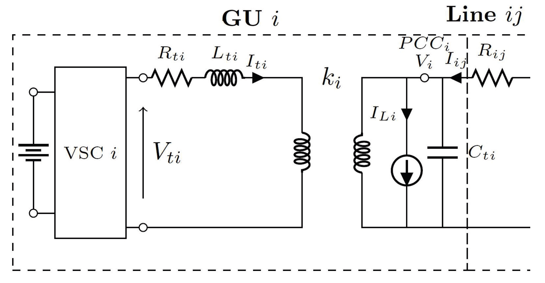
In this section, the dynamical model of the GU for a local power plant is presented. To simplify the analysis process, the realistic model of GU is assumed to consist of transformers, associated filters, and voltage source converters (VSCs) [21]. As shown in Figure 1, through a non-zero impedance three-phase line with ( R i j , L i j ) , the considered GU denoted by i is connected with other units j. The GU is made up of a VSC, a DC voltage source (representing a biomass or waste incineration unit), an inductance L t , a series filter characterized by a resistance R t , and a station step-up transformer ( Y Δ ) ; further, at the point of common coupling (PCC) of the electrical network, the GUs are connected with each other through the transformer, where the transformer coefficients are represented by R t and L t , and k is defined as the transformation ratio.
For the local loads that are connected to the PCC, consider the case where the GU proves the real and reactive powers. Suppose that the loads are time-varying and unknown, and the load current I L is treated as the disturbance for the GU. At the PCC of each local area, the effect of high-frequency harmonics of the load voltage is attenuated by using the shunt capacitance C t . In the abc-frame, based on the dynamical equations of this scheme and by applying Park’s transformation, the model rotating with speed ω 0 in the d q -frame is obtained as follows:
G U i : d V i , d q d t + j ω 0 V i , d q = k i C t i I t i , d q + 1 C t i I t i , d q 1 C t i I L i , d q d I t i , d q d t + j ω 0 I t i , d q = R t i L t i I t i , d q k i L t i V i , d q + 1 L t i V t i , d q
L i n e i j : d I i j , d q d t + j ω 0 I i j , d q = 1 L i j V j , d q R i j L i j I i j , d q 1 L i j V i , d q
where V i , d q is the output voltage at the PCC, and V t i , d q and I t i , d q are the output voltage and current of the GU, respectively. The states in (1) and (2) can be divided into two segments—that is, the d q reference frame is divided as the real component d- and the imaginary component q-, respectively, and I i j is the line current. Modeling the load current I L i , d q as the disturbance, (1) and (2) can be represented through the following continuous time linear dynamic form:
x ˙ ( t ) = A x ( t ) + B u ( t ) + E ω ( t ) y ( t ) = C x ( t ) + v ( t )
where x = [ V i , d , V i , q , I t i , d , I t i , q , I i j , d , I i j , q ] T is the state vector, u = [ V t i , d , V t i , q , V t j , d , V t j , q ] T is the control input, ω = [ I L i , d , I L i , q , I L j , d , I L j , q ] T is the unknown disturbance, y = [ V i , d , V i , q , V j , d , V j , q ] T is the measurement output, and v ( t ) is the measurement noise. Suppose that ω ( t ) and v ( t ) are bounded, where ω ( t ) δ ω , v ( t ) δ v . A, B, C, and E are system matrices to be determined later. This model is regarded as the master model here, since the states of the line are controlled by the GU i only for the control purpose.
To isolate the effects of other connected GUs on the grid, an approximate model is given to avoid the requirement of applying the line current in the GU’s dynamic equations. Let d I i j , d q d t = 0 ; the quasi-stationary line approximations model is given as
I ¯ i j , d q = V j , d q ( R i j + j ω 0 L i j ) V i , d q ( R i j + j ω 0 L i j ) .
Then, replace variable I i j , d q in (2) and divide the complex d q quantities into the corresponding d and q components; the transformed model for GUi is formulated as follows:
G U i : d V i , d d t = ω 0 V i , q + k i C t i I t i , d 1 C t i I L i , d + 1 C t i I ¯ i j , d d V i , q d t = ω 0 V i , d + k i C t i I t i , q 1 C t i I L i , q + 1 C t i I ¯ i j , q d I t i , d d t = k i L t i V i , d R t i L t i I t i , d + ω 0 I t i , q + 1 L t i V t i , d d I t i , q d t = k i L t i V i , q R t i L t i I t i , q ω 0 I t i , d + 1 L t i V t i , q
then, the dynamic model (1) of the GU is constructed as the following state space model form:
A = 1 C t i ( R i j Z i j 2 ) ω 0 1 C t i ( X i j Z i j 2 ) k i C t i 0 ω 0 + 1 C t i ( X i j Z i j 2 ) 1 C t i ( R i j Z i j 2 ) 0 k i C t i k i L t i 0 R t i L t i ω 0 0 k i L t i ω 0 R t i L t i , B = 0 0 0 0 1 L t i 0 0 1 L t i ,
C = 1 0 0 0 0 1 0 0 0 0 1 0 0 0 0 1 , E = 1 C t i 0 0 1 C t i 0 0 0 0 .
where X i j = ω 0 L i j , Z i j = R i j + j X i j , x ( t ) = [ V i , d , V i , q , I t i , d , I t i , q ] T , u ( t ) = [ V t i , d , V t i , q ] T , and ω ( t ) = [ I L i , d , I L i , q ] T .

2.2. Control Framework

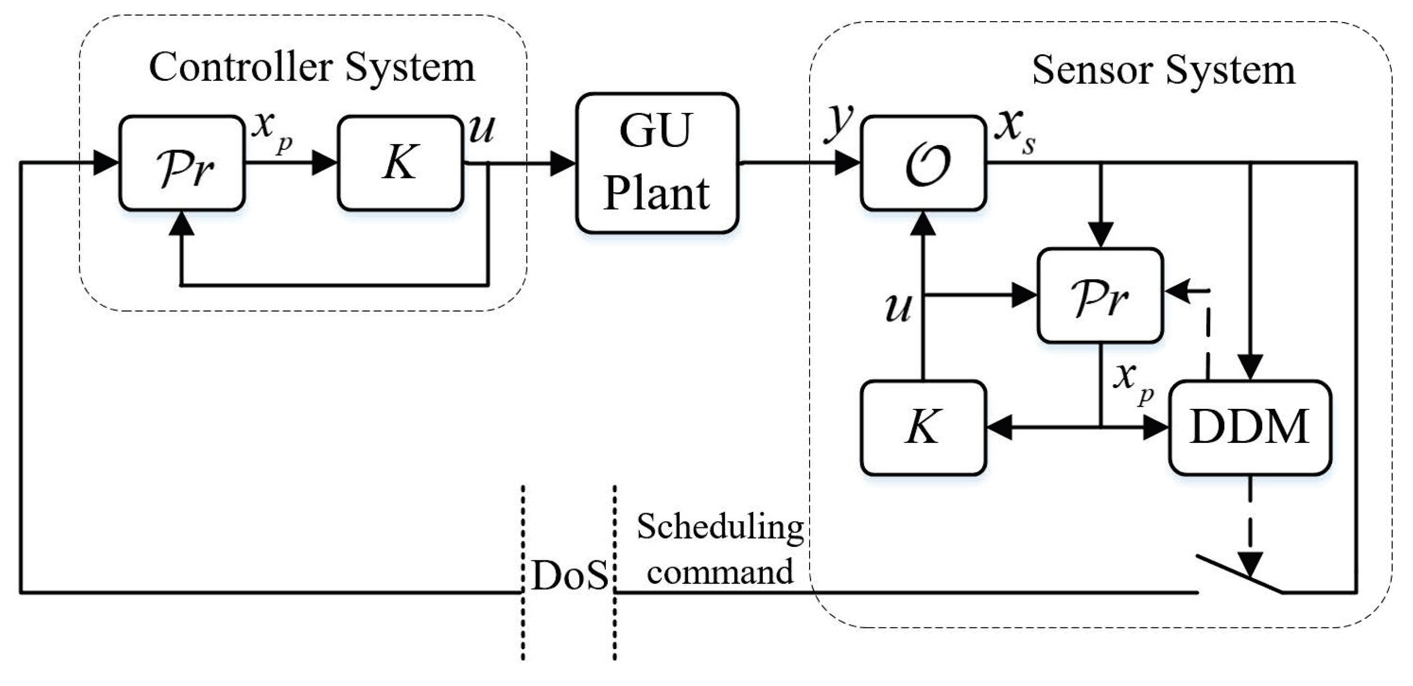
In order to meet the scheduling and control practice based on the network communication while guaranteeing the desirable scheduling performance of the GU, the control construction is designed as in Figure 2. A sensor system is designed to transmit the measurement information to the remote controller system based on the communication network. At the same time, the network communication is unreliable, which is caused by DoS attacks.
The smart sensor system with a demand-driven method and periodic verification strategy is designed to schedule the scheduling commands. The sensor system consists of an observer O that deals with disturbance and noise, and the time when information is needed to be sent to the controller system is decided by a designed DDM. Furthermore, the controller system contains a predictor P r that can compensate the GU’s state data loss during the transmission interval using the latest received data. To suppress the impact of disturbance and noise, the H observer is designed as follows:
O b s e r v e r O : x ˙ s ( t ) = A x s ( t ) + B u ( t ) + L ( y ( t ) C x s ( t ) ) + L v ( t )
where x s ( t ) denotes by the state estimation of the sensor system and L is the designed gain matrix. Denote e s ( t ) = x ( t ) x s ( t ) by the observation error; then, the error dynamic can be formulated as
e ˙ s ( t ) = Φ L e s ( t ) + Γ ξ ( t )
where Φ L = A L C , Γ = [ I L ] , ξ ( t ) = E ω ( t ) v ( t ) . Based on continuous-time systems’ bounded real lemma [23], the gain matrix L is able to be calculated based on the LMI in (7) and e s ( t ) 2 < γ ξ ( t ) 2 is obtained.
P ¯ Φ L + Φ L T P ¯ P ¯ Γ I γ I 0 γ I < 0
where P ¯ is a symmetric positive definite matrix and γ is a small positive scalar, which represents the H performance index. The predictor is given as
P r e d i c t o r P r : x ˙ p ( t ) = A x p ( t ) + B u ( t ) , x s ( t ) i s n o t r e c e i v e d x p ( t ) = x s ( t ) , x s ( t ) i s r e c e i v e d .
Whether the observer data x s ( t ) are sent is determined by the demand of scheduling control, which is represented by the difference between the observed states of the GU and the predicted value of the remote controller. Then, the DDM is designed as follows:
x s ( t ) i s s e n t x s ( t ) x p ( t ) > σ s x s ( t ) + σ c ρ
where ρ = γ C δ + δ v , δ = E δ ω + δ v , σ s and σ c are suitable positive demand parameters to be selected later, and γ is obtained by solving LMI (7). Besides, when the DDM (9) is met, an acknowledgment (ACK) signal is required to affirm that the transmission attempt was successful, and this assumption is consistent with the TCP-type communication protocol.
Define t k k N 0 as the sequence performing data transmission of control update, and denote Δ k = t k + 1 t k by the data transmission interval between two consecutive attempts, which
0 < Δ ̲ Δ k Δ ¯
where Δ ¯ and Δ ̲ are upper and lower bounds of the intervals between two consecutive attempts, respectively.
Remark 1. 
The length of interval Δ k is decided by the DDM (9), but it is necessary to set the lower and upper bound. Due to the characteristic of periodic verification strategy, the lower bound Δ ̲ can be selected as the DDM verification period. Inspired by the pre-specified upper bound of inter-event times in [17], the upper bound Δ ¯ is needed to force the sensor to send data to the remote controller if the transmission is not executed for long periods of time.
The sensor system transmits the latest estimation value x s ( t ) to the controller system by network communication to renew the state prediction x p ( t ) at t k k N 0 —that is, x p ( t k ) = x s ( t k ) , and it is the initial value for the state prediction when t [ t k , t k + 1 ) . Then, x p ( t ) is calculated by (8) and the control value is able to be designed by the switching controller formulated as
u ( t ) = K x p ( t ) , x s ( t ) i s n o t r e c e i v e d K x s ( t ) , x s ( t ) i s r e c e i v e d .
where K is the state feedback gain matrix. In order to improve the rate of convergence, region poles assignment lemma [23] is used to solve K with α stability margin. Let Φ 2 = A + B K ; then, K can be obtained by solving the following LMI:
P 2 Φ 2 + Φ 2 T P 2 + 2 α P 2 < 0
where α > 0 is a given coefficient and P 2 is a symmetric positive definite matrix.
As in Figure 2, a replica of the predictor P r is run in the sensor system so that it can synchronize x p ( t ) that the controller system has and can judge whether (9) is satisfied. When the DDM (9) is not satisfied, x s ( t ) is not sent and the error between x p ( t ) and x s ( t ) is accumulated until (9) is satisfied; then, x s ( t ) is transmitted to the predictor P r , and an ACK signal is sent and returned to the sensor from the controller system by the network to ascertain that the transmission attempt was triumphant.

3. Demand-Driven Control Strategy

This section gives the design process of the demand-driven control strategy—that is, the selection method of driven parameters under the premise of ensuring the control objective. First of all, the control objective is described as the definition provided below:
Definition 1 
([24]). Given the GU system (3) with control input (11), for each ω t L ( R , ω 0 ) and x ( 0 ) R n , if there is a K L -function h 1 ( · ) and a K -function h 2 ( · ) such that
x ( t ) h 1 ( x ( 0 ) , t ) + h 2 ( ω t )
holds for all t R with t 0 , the system is considered to be ISS. Besides, the system (3) is globally asymptotically stable if (13) is satisfied for ω t 0 .
Then, the design process of the demand-driven parameters is given. For t R , t 0 , to measure the difference between the truth state x ( t ) and the state prediction x p ( t ) , which represents the demand of network communication, denote the prediction error by
e ( t ) = x p ( t ) x ( t )
Then, the formula for the closed-loop GU system is given as
x ˙ ( t ) = Φ 2 x ( t ) + B K e ( t ) + E ω ( t )
Design the Lyapunov function as V ( t ) = x T ( t ) P x ( t ) , where P is the unique solution of the following Lyapunov equation:
P Φ 2 + Φ 2 T P + Q = 0
where Q is any given positive definite symmetric matrix. Then, we have
α 1 x ( t ) V ( t ) α 2 x ( t )
V ˙ ( t ) γ 1 x ( t ) 2 + γ 2 x ( t ) e ( t ) + γ 3 x ( t ) ω ( t )
for any t R , t 0 , where α 1 and α 2 are equal to the smallest and largest eigenvalues of P, respectively. γ 1 is the smallest eigenvalue of Q; γ 2 = 2 P B K and γ 3 = 2 P E . Notice that x s ( t ) x p ( t ) σ s x s ( t ) + σ c ρ is always true when t [ t k , t k + 1 ) ; then, it yields
x ( t ) x p ( t ) σ s x ( t ) + σ c ρ + λ ξ ( t )
where the inequality comes from the triangle inequality and the fact that e s ( t ) = x ( t ) x s ( t ) < γ ξ ( t ) . Then, ξ ( t ) E δ ω + δ v = δ yields
e ( t ) = x ( t ) x p ( t ) σ s x ( t ) + σ δ δ
where σ δ = γ σ c C + γ + σ c . Then, V ˙ ( t ) ( γ 1 σ s γ 2 ) x ( t ) 2 + ( γ 3 + σ δ γ 2 ) x ( t ) δ can be obtained by substituting (20) into (18) and indicates that when γ 1 σ s γ 2 > 0 holds,
V ( x ( t ) ) e θ 1 t V ( x ( 0 ) ) + γ 4 δ 2
where θ 1 = γ 5 2 α 1 , γ 4 = ( γ 3 + σ δ γ 2 ) 2 2 γ 5 θ 1 , and γ 5 = γ 1 σ s γ 2 .
The use of the prediction method makes the controller system able to simulate the true state value; then, the discrepancy accumulated in the transmission interval is degraded by the information compensation. From (14), it yields for any t [ t k , t k + 1 ) that the dynamic of the prediction error can be formulated as
e ˙ ( t ) = x ˙ p ( t ) x ˙ ( t ) = A e ( t ) E ω ( t )
then, we have the upper bound of the error as
e ( t ) t k t e μ A ( t τ ) ( A e s ( t k ) + E ω ( τ ) ) d τ < f ( t t k ) ( γ A δ + E δ ω ) = ε ( γ A δ + E δ ω )
where f ( t t k ) = t k t e μ A ( t τ ) d τ and ε = Δ k , μ A 0 1 μ A ( e μ A Δ k 1 ) , μ A > 0 .
Because the DDM (9) is periodically validated in the case of a continuous system process, it is necessary to investigate the transmission attempt sequence { t k } k N 0 to eliminate continuous transmissions within each validation period. Denote the estimation–prediction error by e p ( t ) = x s ( t ) x p ( t ) ; then, the dynamic of this error is
e ˙ p ( t ) = A e p ( t ) + L y ¯ ( t )
where y ¯ ( t ) = C e s ( t ) + v ( t ) . Since e p ( t k ) = 0 for any t [ t k , t k + 1 ) , it yields
e p ( t ) L t k t e μ A ( t τ ) y ¯ ( τ ) d τ L t k t e μ A ( t τ ) d τ ( C e s ( t ) + v ( t ) ) ρ L ( t t k ) , μ A 0 ρ L μ A ( e μ A ( t t k ) 1 ) , μ A > 0
where ρ = γ δ C + δ v as in (9); further, it yields that if t t k Δ ̲ with
Δ ̲ = σ c L , μ A 0 1 μ A log ( μ A σ c L + 1 ) , μ A > 0
then for any σ c > 0 , the DDM (9) cannot be satisfied if t [ t k , t k + Δ ̲ ) .
Remark 2. 
Notice that the threshold part of the mechanism is divided into two items. One influences the stability of the system and is determined by the parameter σ s . If the selected parameter σ s is large, the demand error will be too large compared to the updated data x s ( t ) , and the updated data may not stabilize the system. The other parameter is σ c , which determines the influence of the disturbance and noise to the DDM. The selection of σ c directly determines the minimum transmission interval Δ ̲ , and σ c can be chosen based on the quantitative relationship (25).

4. Resilient Control with Unreliable Communication

Notice that when the demand-driven control strategy is designed, the status of the communication is unknown. In other words, the prediction-based control algorithm is a passive resilient scheme. When a DoS attack occurs, the active communication scheduling protocol is another resilient scheme, which is presented in this section. Besides, the stability analysis under DoS attacks is given.

4.1. DoS Attack Model

To extend the application range of resilient control as far as possible, the unreliable communication caused by DoS attacks is considered here, and a general attack model is adopted that restricts the attack behavior by only posing constraints in time on their duration and frequency. Denote d n n N 0 by the DoS off/on transitions sequence with d 0 0 —that is, the time instant set in which attack behavior turns from zero (communication channel is reliable) to one (transmissions are jammed). The nth DoS time-interval is D n = d n [ d n , d n + τ n ) , and τ n R , τ n 0 is the length. Then, D n is a single pulse if τ n = 0 . Suppose that D n n N has no overlap; then, consider an interval [ t , ζ ) with 0 t < ζ and let
D ( t , ζ ) = n N 0 D n [ t , ζ )
H ( t , ζ ) = [ t , ζ ) D ( t , ζ )
be the subset of time intervals in [ t , ζ ) where the network is in attack status and healthy, respectively. Denote n ( t , ζ ) by the number of DoS off/on transitions over [ t , ζ ) . Referring to [10], the following assumptions are proposed to restrict the frequency and duration of DoS attacks.
Assumption A1. 
For any 0 t < ζ , there exist scalars κ R , η 0 and τ D R , τ D Δ ̲ such that
n ( t , ζ ) κ + ζ t τ D
Assumption A2. 
For any 0 t < ζ , there exist scalars ς R , ς 0 and T R , T > 1 such that
D ( t , ζ ) ς + ζ t T
Remark 3. 
The frequency and duration assumptions for DoS attacks are necessary. Take into account the worst scenario without the limitations: firstly, if n ( t , ζ ) is sufficient large, each transmission attempt may be overridden by attack pulses; secondly, when D ( t , ζ ) is sufficient large, an attack interval may never stop in any given [ t , ζ ) . In both cases, all the transmissions can be jammed and the scheduling control performance cannot be guaranteed. Besides, the two assumptions can be understood in terms of attack energy. Assume that an attacker having confined energy to carry out attack behaviors is reasonable and the usable energy is proportional to the length of time interval [ t , ζ ) with a scale factor. The energy expended by each attack off/on transition is τ D , and for each unit of time, the required energy to sustain an attack execution is T. Furthermore, κ and ς can be considered as regularized scalars.

4.2. Control Update Protocol Under DoS Attacks

Define the first time instant where the DDM is verified to be true after a data communication success at t k as
λ k = inf { t R , t > t k | x s ( t ) x p ( t ) σ s x s ( t ) + σ c ρ }
If a data transmission appears in an attack interval D n , the attempt cannot be successful. Define F = { k N 0 | t k n N 0 D n } as the set of integers associated with communication attempts that occur under attack. During the attack intervals, the control strategy of the GU system is converted to a periodic communication protocol—that is, the selected communication attempt period is smaller than or equal to the demand-driven control scheduling interval for the purpose of decreasing the communication delay introduced by the jamming attack. For any k N 0 , the time when that communication attempt occurs is described below:
t k + 1 = t k + Δ * , i f k F t k + Δ ¯ , i f k F Δ ¯ < λ k t k λ k , otherwise
where the control update period during the jamming attack intervals is denoted by Δ * , which satisfies 0 < Δ * Δ ̲ .
Remark 4. 
Equation (31) provides the resilient update protocol against the jamming attack behaviors described in Assumptions 1 and 2. If the sensor can receive the ACK signal at t k , then the data transmission at t k succeeds. Then, the next data transmission will be attempted at λ k when Δ ¯ λ k t k . If Δ ¯ < λ k t k , then the next data transmission will be attempted at t k + Δ ¯ . If the ACK signal cannot be received at t k for the sensor, it indicates that an attack off/on transition appeared before t k , and from t k , the data communication is performed at the periodic update rate appointed by Δ * tentatively until the sensor is able to receive the ACK signal again.
Remark 5. 
The resilience is achieved based on an active and passive combined control scheme. First, the predictor provides predicted values as close as possible to the state of the system when there is no data transmission. In this way, when malicious communication interferences occur and data cannot be transmitted, the predictor can compensate for the missing data, thereby improving resilience to unreliable communications actively. Meanwhile, the resilient update protocol designed in this paper is able to minimize the additional transmission periods caused by communication interruptions, so that the system can resume data transmission as early as possible at the end of the attack. This is a passive resilience improvement method.
Define H ^ ( t 1 , t 2 ) as the union of time subintervals in which the DDM (9) is not held in [ t 1 , t 2 ) with 0 t 1 < t 2 —i.e., the union of healthy subintervals in [ t 1 , t 2 ) —and define the union of valid attack subintervals in which DDM (9) is true as D ^ ( t 1 , t 2 ) ; then, the disjoint union of H ^ ( t 1 , t 2 ) and D ^ ( t 1 , t 2 ) is the whole interval [ t 1 , t 2 ) for any 0 t 1 < t 2 , and D ^ ( t 1 , t 2 ) = [ t 1 , t 2 ) H ^ ( t 1 , t 2 ) . Denote
ρ n = 0 , i f F = t sup { k F } d n , o t h e r w i s e
Λ n = 0 , i f F = Δ sup { k F } = Δ * , o t h e r w i s e
then, H ^ n = { d n } [ d n , d n + ρ n + Λ n ) is the n-th effective attack subinterval. It is worth noting that H ^ n and H ^ n + 1 may overlap since d n + 1 may be located in H ^ n . For convenience, the two overlapped subintervals can be considered as an incorporative, effective attack interval. Define { ϕ m } m N 0 as the sequence of off/on transitions of the m-th effective attack interval—that is,
ϕ 0 = d 0 , ϕ m + 1 = inf { d n > ϕ m | d n > d n 1 + ρ n 1 + Λ n 1 }
and the length of the m-th effective attack interval is ν m = n N 0 ϕ m d n < ϕ m + 1 H ^ n H ^ n + 1 ; then, D ^ ( t 1 , t 2 ) = m N 0 [ ϕ m , ϕ m + ν m ) [ t 1 , t 2 ) and H ^ ( t 1 , t 2 ) = m N 0 [ ϕ m + ν m , ϕ m + 1 ) [ t 1 , t 2 ) . From Assumptions 1 and 2, it can be obtained that the upper bound of the time interval for the impact of an attack is
D ^ ( t 1 , t 2 ) D ( t 1 , t 2 ) + ( n ( t 1 , t 2 ) + 1 ) Δ ς + t 2 t 1 T
where ς = ς + ( η + 1 ) Δ and 1 T = Δ τ D + 1 T . The following lemma gives a quantitative characterization of the interval between two successive successful transmissions.
Lemma 1. 
Define { z m } m N 0 as the time sequence at which the data transmissions succeed. For the communication update protocol as in (31), and considering the DoS attacks satisfying Assumptions 1 and 2, z m + 1 z m Ω + Δ ¯ holds for z 0 Ω , where Ω = ( ς + κ Δ ) ( 1 Δ τ D 1 T ) 1 .
Remark 6. 
Inspired by a similar result in [11], the above lemma gives an upper bound on the interval between two successful transmissions with a demand-driven strategy. Since the inner-demand interval is unknown, the time interval between transmission attempts during D n is also unknown. Fortunately, based on the known upper bound of the communication interval Δ ¯ , the worst case of the data updates can be bounded. Evidently, 1 T < 1 is necessary, and it is the loosest restriction to achieve closed-loop stability under any DoS attacks satisfying Assumptions 1 and 2, as discussed in [11].
According to Lemma 1, (22) and (23) yield the upper bound of the prediction error e ( t ) as
e ( t ) < ε ¯ ( γ A δ + E δ ω )
for any t [ z m , z m + 1 ) , where ε ¯ = Ω + Δ ¯ , μ A 0 1 μ A ( e μ A ( Ω + Δ ¯ ) 1 ) , μ A > 0 . It indicates that the prediction error between x p ( t ) and x ( t ) is bound even under DoS attacks. By applying (36), we have the main results as the following theorem.
Theorem 1. 
Consider the GU system (3) with a control structure that consists of the observer O and the predictor P r , the scheduling control input (11), and the DDM (9), and select the parameters such that γ 1 σ s γ 2 > 0 holds. Under Assumptions 1 and 2, if for any DoS attacks with arbitrary scalars ς, κ, τ D , and T such that
Δ τ D + 1 T < 1
holds, where Δ is a positive constant and satisfies Δ Δ ¯ , then the GU control system is ISS with the periodic update protocol (31).
Proof. 
The proof is provided in Appendix A. □
Remark 7. 
The conservatism of the results in [10,20] results from decomposing the timeline into attack intervals and non-attack intervals. In fact, the attack intervals can also be decomposed into valid attack intervals and invalid attack intervals; the latter are the subintervals where the DDM has not been met—that is, x s ( t ) x p ( t ) < σ s x s ( t ) + σ c ρ . The actual effective attack intervals are the subintervals where the DDM is verified to be true and the data transmissions fail. Due to the unknown time at which the attack behavior’s off/on transition occurs, the conservatism of the resilience cannot be decreased by splitting the timeline. Based on the maximum disturbance–accumulation error, which is calculated from (36), the procedure can be understood in turn as the difference converging from the maximum error to σ s x s ( t k ) + σ c ρ with k = inf { k F | t k n N 0 D n } ; in this way, the optimal bound of the tolerable intensity of a DoS attack can be achieved.

5. Simulation Examples

In this section, the GU model constructed in Section 2.1 is applied to validate the resilient control performance of the designed methods. The parameters of the GU system are shown as follows: f 0 = 1 Hz , ω 0 = 6.283 rad / s , R i j = 1.3 × 10 3 Ω , C t i = 62.86 F , k i = 0.0435 , L i j = 0.6 H , L t i = 9.26 × 10 3 H , R t j = 1.3 × 10 3 Ω . The system matrices of the GU model can be calculated as follows:
A = 1.3 2.516 0.691 0 2.516 1.3 0 0.691 4.69 0 0.14 6.283 0 4.69 6.283 0.14 , B = 0 0 0 0 1.07 0 0 1.07 , C = 1 0 0 0 0 1 0 0 0 0 1 0 0 0 0 1 .
In the simulation, the unknown disturbance ω ( t ) is assumed as stochastic signals with a uniform distribution in [ 0.4 , 0.4 ] and noise v ( t ) is v ( t ) = a sin ( Ω y ) , Ω y [ 0 , 2 π ] , where a is a stochastic number with a uniform distribution bounded in [ 0 , 0.2 ] . The initial conditions are x ( 0 ) = x p ( 0 ) = [ 0.8 , 1 , 0 , 0.3 ] T . The control objective is to track the reference signal [ 0.08 0.09 0.12 0.63 ] T . Selecting λ = 5.97 , the gain matrices of observer and controller can be calculated by solving the LMIs (7) and (12) as follows:
L = 0.5755 0.5755 0.1981 3.8506 1.1000 3.8657 5.5976 6.8427 , K = 0.0630 0.2771 0.3848 0.0003 0.2788 0.1109 0.0003 0.3278 .
The relative parameters can be obtained such that Φ 2 = 8.1528 , α 1 = 1.4768 , α 2 = 0.3375 , γ 1 = 1 , γ 2 = 1.4976 , and γ 3 = 2.9536 . Thus σ s has to be chosen such that σ s < 0.6677 . Setting σ s = 0.66 , and Δ ¯ = 0.5 s and Δ ̲ = 0.01 s, the demand-driven parameter σ c is chosen as σ c = 0.004 
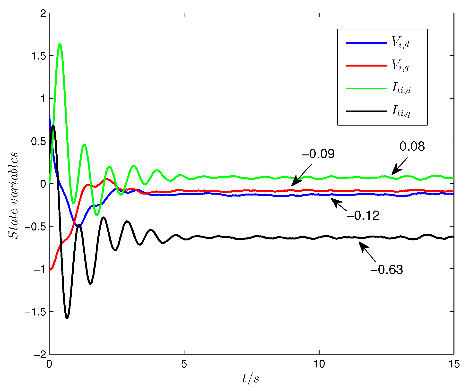
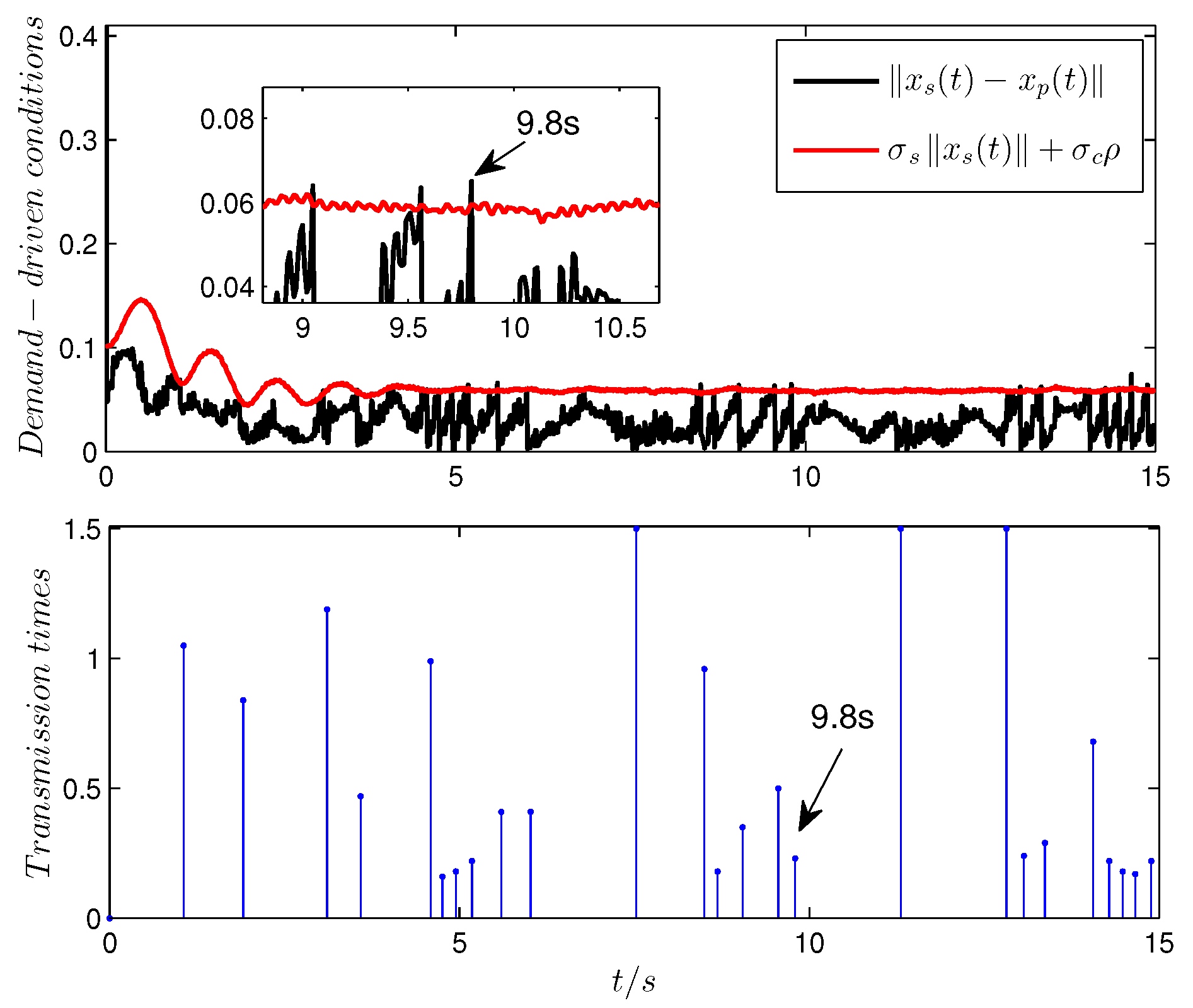
. When there are no DoS attacks, the state responses of the controlled system, the evolution of the transmission times, and the demand-driven conditions x s ( t ) x c ( t ) and σ s x s ( t ) + σ c ρ are exhibited in Figure 3 and Figure 4, respectively. From the above figures, it is obvious that the demand-driven control algorithm is able to ensure that the state responses of the GU system track the reference values while the number of network transmissions is decreased significantly. From Figure 4, when the demand (black) exceeds the transmission condition (red), the data are transmitted over the network (such as at 9.8 s). The black line quantifies the information difference between the controller side and the sensor side, which represent the control requirements in real application scenarios. The red line quantifies the acceptable demand threshold. If the information difference does not exceed the threshold, it indicates that the impact of the difference on system performance during actual application is tolerable, and no data transmission is required.
When DoS attacks occur, the transmission protocol is provided in (31), and the transmission attempt period is Δ = 0.01 s. In the simulation time domain of 15 s, the DoS attack is executed randomly and satisfies n ( 0 , 15 ) = 12 and D ( 0 , 15 ) = 10.93 s. According to the duration and frequency of the attack, we have τ D 1.25 and T 1.372 ; then, Δ τ D + 1 T 0.737 
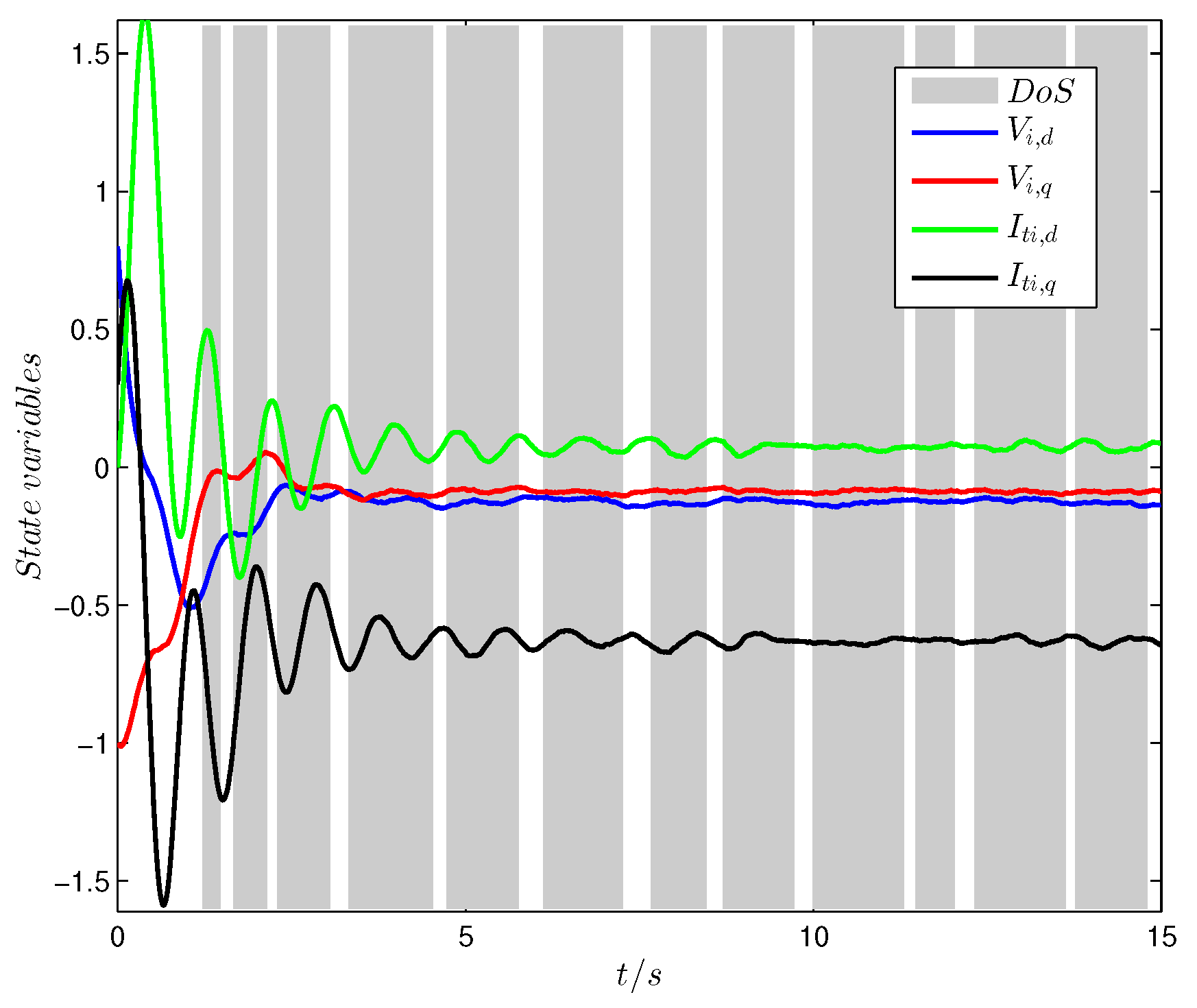
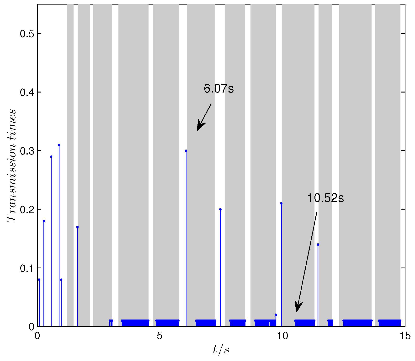
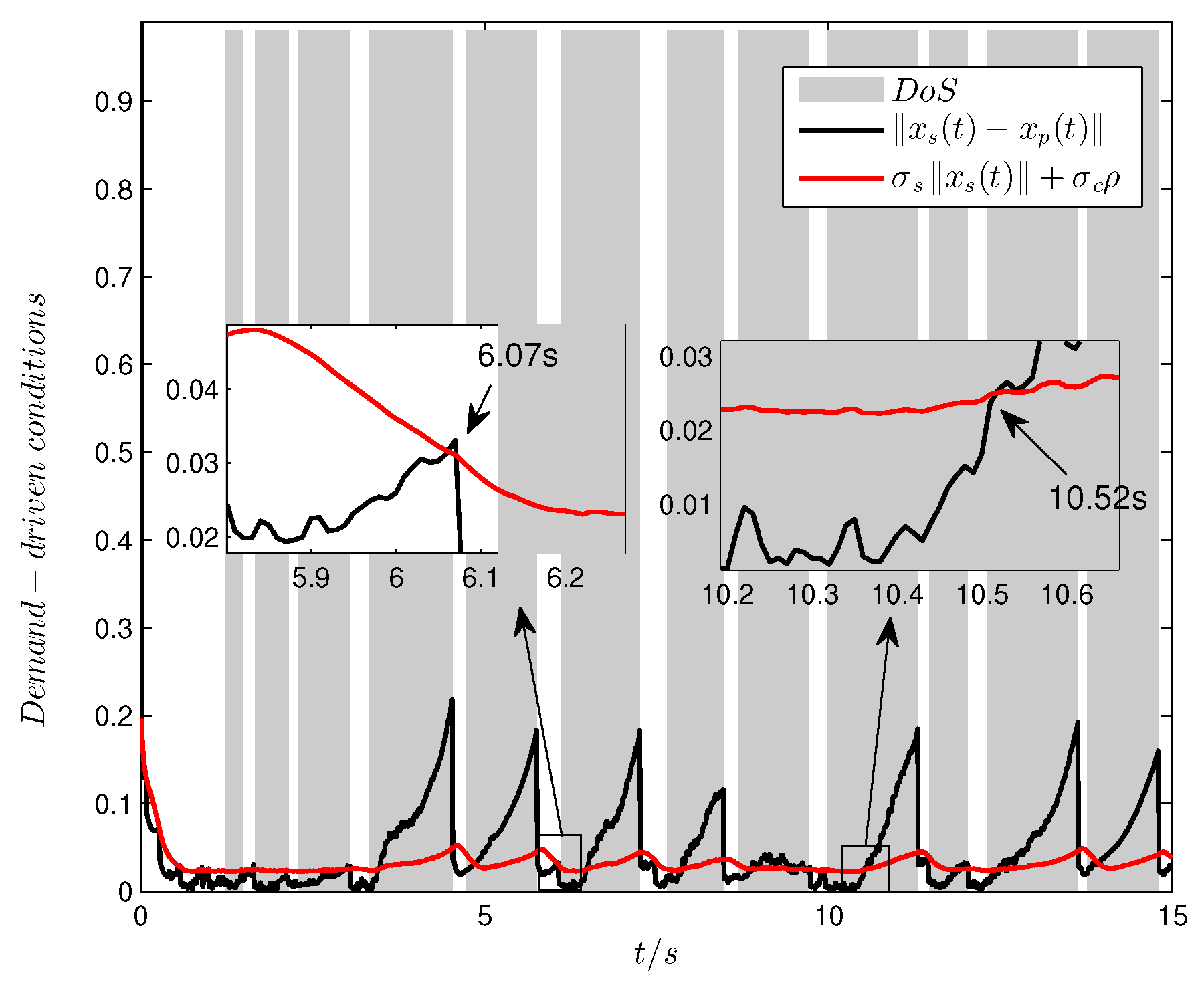
. Then, the state responses of the closed-loop GU system, the evolution of the transmission times, and the demand-driven condition x s ( t ) x p ( t ) and σ s x s ( t ) + σ c ρ are exhibited in Figure 5, Figure 6 and 
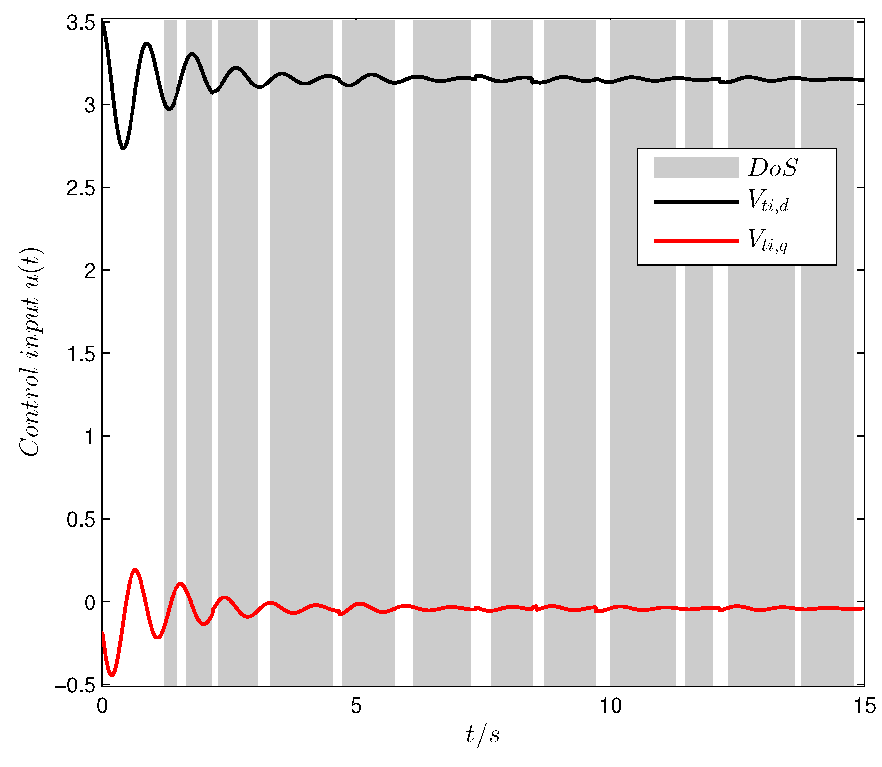
Figure 7, respectively. Finally, the control input of the GU model is given in Figure 8.
From Figure 5, it can be observed that the states of the GU model can also track the reference values under DoS attacks. However, compared with Figure 3 and Figure 5, it is shown that the time it takes for the wave of states under DoS attacks to end is significantly longer than that without DoS attacks, which indicates the influence of the DoS attacks to the networked control strategy. As can be observed from Figure 6 and Figure 7, the demand-driven algorithm still works, and the transmission attempts succeed during the no-attack intervals when the demand exceeds the transmission condition (such as at 6.07 s) while the transmission mode switches to periodic attempts during the attack intervals (such as 10.52 s). As can be seen from the above figures, the demand-driven control scheme also has a certain potential resilience in practical applications. For instance, from Figure 7, it can be seen that the DoS attacks before the demand (black) exceeds the threshold (red) are invalid. In these intervals, there is no transmission attempt, which can be observed in Figure 6 before 10.52 s.

6. Conclusions

This paper focuses on the secure control problem for the GU of a local power plant under unreliable communication, and the demand-driven control strategy has been investigated. The unreliable communication in consideration is caused by DoS attacks, and the resilient control algorithm is designed to handle the problem of performance degradation in this scenario. An H observer-based prediction method is provided, and the DDM is designed based on the error between the state estimation and prediction. In this way, the communication resources are saved while the ideal scheduling control performance is obtained. Based on the ISS analysis, the sufficient conditions on the DoS attack model are provided to ensure the stability of the GU system. Finally, simulation results were presented to demonstrate the effectiveness of the designed methods.
The technical novelties are summed up as follows: First, the H observer-based prediction method is able to remove the influence of unknown load currents to the system and compensate the loss of state data in the interval between any two continuous transmissions of scheduling signals. Second, the advanced demand-driven strategy with periodic verification is presented to schedule the intermittent communication. Third, by using the thought of robustness to the maximum disturbance-induced error, the conservatism of the tolerable attack intensity is decreased.

Author Contributions

Conceptualization, G.C. and D.X.; methodology, Y.-C.S.; software, Z.W.; validation, D.X. and B.L.; formal analysis, G.C. and D.X.; investigation, Y.-C.S.; resources, K.M.; data curation, B.L. and K.M.; writing—original draft preparation, Y.-C.S.; writing—review and editing, G.C. and Y.-C.S.; visualization, Y.-C.S.; supervision, G.C. and D.X.; project administration, G.C. and Z.W.; funding acquisition, G.C. and D.X. All authors have read and agreed to the published version of the manuscript.

Funding

This work was supported in part by the State Grid Henan Electric Power Company Technology Project (Grant No. 521702240003).

Data Availability Statement

Dataset available on request from the authors.

Conflicts of Interest

Author Guizhou Cao, Dawei Xia and Kai Meng was employed by the company State Grid Henan Electric Power Company. The remaining authors declare that the research was conducted in the absence of any commercial or financial relationships that could be construed as a potential conflict of interest.

Appendix A

Proof of Theorem 1.
Firstly, a stability analysis of the effective attack subinterval [ ϕ m , ϕ m + ν m ) and the healthy subinterval [ ϕ m + ν m , ϕ m + 1 ) is provided.
Select the Lyapunov function as V ( t ) = x T ( t ) P x ( t ) , where P and Q are calculated as in (16). It is worth noting that x ( t ) x p ( t ) σ s x ( t ) + σ c ρ holds for all t [ ϕ m + ν m , ϕ m + 1 ) , m N 0 ; then, from (21), we have
V ( x ( t ) ) e θ 1 ( t ϕ m ν m ) V ( x ( ϕ m + ν m ) ) + γ 4 δ 2
where θ 1 = γ 5 2 α 1 , γ 4 = γ 3 2 2 γ 5 θ 1 , and γ 5 = γ 1 σ s γ 2 .
Then, the effective attack interval t [ ϕ m , ϕ m + ν m ) , m N 0 is concerned. Beginning at some point in the above interval, x ( t ) x p ( t ) σ s x ( t ) + σ c ρ will become false. From (36), it yields that e ( t ) < ε ¯ ( γ A δ + E δ ω ) holds; then, from (18), we have
V ˙ ( x ( t ) ) γ 1 x ( t ) 2 + γ 2 ε ¯ x ( t ) ( γ A δ + E δ ω ) + γ 3 x ( t ) E ω ( t ) γ 1 x ( t ) 2 + ( γ 2 ε ¯ + γ 3 ) x ( t ) δ e
where δ e = γ A δ + E δ ω . Then, based on Yang’s inequality, it yields
V ˙ ( x ( t ) ) γ 1 2 x ( t ) 2 + ( γ 2 ε ¯ + γ 3 ) 2 2 γ 1 δ e 2 θ 2 V ( x ( t ) ) + γ 6 δ e 2
where θ 2 = γ 1 2 α 1 , γ 6 = ( γ 2 ε ¯ + γ 3 ) 2 2 γ 1 ; thus, it can be calculated that
V ( x ( t ) ) e θ 2 ( t ϕ m ) V ( x ( ϕ m ) ) + γ 7 δ e 2
holds for all t [ ϕ m , ϕ m + ν m ) , m N 0 , and γ 7 = γ 6 θ 2 .
Secondly, stability analysis on the entire timeline is given. For any t R , t > 0 , it yields
V ( x ( t ) ) e θ 1 H ^ ( 0 , t ) e θ 2 D ^ ( 0 , t ) V ( x ( 0 ) ) + γ m N 0 ; ϕ m t e θ 1 H ^ ( ϕ m + ν m , t ) e θ 2 D ^ ( ϕ m , t ) δ 2
where γ = max { γ 4 , γ 7 } and δ = max { δ , δ e } . Based on (35), one can obtain that for any t R , t > ϕ m , D ^ ( ϕ m , t ) ς + t ϕ m T holds. When t < ϕ m + ν m , we have that D ^ ( τ , t ) = [ t 1 , t 2 ] H ^ ( t 1 , t 2 ) and H ^ ( ϕ m + ν m , t ) = 0 hold, which yields
H ^ ( ϕ m + ν m , t ) = t ϕ m D ^ ( ϕ m , t )
It is worth noting that D ^ ( ϕ m , t ) = ν m and D ^ ( ϕ m + ν m , t ) = 0 hold for any t R , t > ϕ m + ν m ; then, it is indicated that H ^ ( ϕ m + ν m , t ) = t ϕ m ν m = t ϕ m D ^ ( ϕ m , t ) holds. Then, it yields
m N 0 ; ϕ m t e θ 1 H ^ ( ϕ m + ν m , t ) e θ 2 D ^ ( ϕ m , t ) e ( θ 2 θ 1 ) ς m N 0 ; ϕ m t e a ( t ϕ m )
where a = θ 1 + θ 2 θ 1 T . It is obvious that a > 0 can be guaranteed by 1 T < 1 . Similar to the transformation of (A7), the term e θ 1 H ^ ( 0 , t ) e θ 2 D ^ ( 0 , t ) in the right hand of (A5) can have an upper bound as e ( θ 2 θ 1 ) ς e a t , which yields
V ( x ( t ) ) e ( θ 2 θ 1 ) ς e a t V ( x ( 0 ) ) + γ ( 1 + e ( θ 2 θ 1 ) ς m N 0 ; ϕ m t e a ( t ϕ m ) ) δ 2
Inspired by the result from [10], it yields m N 0 ; ϕ m t e a ( t ϕ m ) e a η τ D 1 e a τ D ; then, we have
x ( t ) α 1 α 2 e ( θ 2 θ 1 ) ς 2 e a t 2 x ( 0 ) + γ α 2 ( 1 + e a κ τ D 1 e a τ D e ( θ 2 θ 1 ) ς ) δ
It is obvious that the scalars of (A9) have no connection with the initial conditions of the dynamic process and the unknown disturbance; then, based on Definition 1, it can be ascertained that the GU control system (3) is ISS. This ends the proof. □

References

  1. Qu, B.G.; Wang, Z.D.; Shen, B.; Dong, H.L. Distributed state estimation for renewable energy microgrids with sensor saturations. Automatica 2021, 131, 109730. [Google Scholar] [CrossRef]
  2. Jonathan, D.; Wang, J.H. AGC signal modeling for energy storage operations. IEEE Trans. Power Syst. 2014, 29, 2567–2568. [Google Scholar]
  3. Tian, J.W.; Wang, B.H.; Li, T.Y.; Shang, F.T.; Cao, K.R. Coordinated cyber-physical attacks considering DoS attacks in power systems. Int. J. Robust Nonlinear Control 2020, 31, 4345–4358. [Google Scholar] [CrossRef]
  4. Deng, R.L.; Gao, G.X.; Lu, R.X.; Liang, H.; Athanasios, V. False data injection on state estimation in power systems–attacks, impacts, and defense: A survey. IEEE Trans. Ind. Inform. 2017, 13, 411–423. [Google Scholar] [CrossRef]
  5. Qi, W.H.; Sha, M.X.; Park, J.H.; Yan, H.C.; Xie, X.P. Asynchronous stabilization for discrete hidden semi-markov jumping power models with cyber attacks. IEEE Trans. Circuits Syst. II Express Briefs 2023, 70, 2565–2569. [Google Scholar] [CrossRef]
  6. Peng, C.; Li, J.C.; Fei, M.R. Resilient event-triggering H-infinity load frequency control for multi-area power systems with energy-limited DoS attacks. IEEE Trans. Power Syst. 2017, 32, 4110–4118. [Google Scholar] [CrossRef]
  7. Li, Y.Z.; Shi, L.; Cheng, P.; Chen, J.M.; Quevedo, D.E. Jamming attacks on remote state estimation in cyber-physical systems: A game-theoretic approach. IEEE Trans. Autom. Control 2015, 60, 2831–2836. [Google Scholar] [CrossRef]
  8. Zhang, H.; Cheng, P.; Shi, L.; Chen, J.M. Optimal denial-of-service attack scheduling with energy constraint. IEEE Trans. Autom. Control 2015, 60, 3023–3028. [Google Scholar] [CrossRef]
  9. Zhang, H.; Cheng, P.; Shi, L.; Chen, J.M. Optimal DoS attack scheduling in wireless networked control system. IEEE Trans. Control. Syst. Technol. 2016, 24, 843–852. [Google Scholar] [CrossRef]
  10. Persis, C.D.; Tesi, P. Input-to-state stabilizing control under denial-of-service. IEEE Trans. Autom. Control 2015, 60, 2930–2944. [Google Scholar] [CrossRef]
  11. Feng, S.; Tesi, P. Resilient control under denial-of-service: Robust design. Automatica 2017, 79, 42–51. [Google Scholar] [CrossRef]
  12. Persis, C.D.; Tesi, P. Networked control of nonlinear systems under denial-of-service. Syst. Control Lett. 2016, 96, 124–131. [Google Scholar] [CrossRef]
  13. Lu, A.Y.; Yang, G.H. Input-to-state stabilizing control for cyber-physical systems with multiple transmission channels under denial-of-service. IEEE Trans. Autom. Control 2018, 63, 1813–1820. [Google Scholar] [CrossRef]
  14. Dolk, V.S.; Tesi, P.; Persis, C.D.; Heemels, W.P.M.H. Event-triggered control systems under denial-of-service attacks. IEEE Trans. Control Netw. Syst. 2017, 4, 93–105. [Google Scholar] [CrossRef]
  15. Qi, W.H.; Sha, M.X.; Park, J.H.; Wu, Z.G.; Yan, H.C. Observer-based asynchronous control of discrete-time semi-Markov switching power systems under DoS attacks. IEEE Trans. Syst. Man Cybern. Syst. 2024, 54, 6424–6434. [Google Scholar] [CrossRef]
  16. Lunze, J.; Lehmann, D. A state-feedback approach to event-based control. Automatica 2010, 46, 211–215. [Google Scholar] [CrossRef]
  17. Zhang, J.H.; Feng, G. Event-driven observer-based output feedback control for linear systems. Automatica 2014, 50, 1852–1859. [Google Scholar] [CrossRef]
  18. Yu, H.; Hao, F. Input-to-state stability of integral-based event-triggered control for linear plants. Automatica 2017, 85, 248–255. [Google Scholar] [CrossRef]
  19. Heemels, W.P.M.H.; Donkers, M.C.F.; Teel, A.R. Periodic Event-triggered control for linear systems. IEEE Trans. Autom. Control 2013, 58, 847–861. [Google Scholar] [CrossRef]
  20. Donkers, M.C.F.; Heemels, W.P.M.H. Model-based periodic event-triggered control for linear systems. Automatica 2013, 49, 698–711. [Google Scholar]
  21. Riverso, S.; Sarzo, F.; Frerrari-Trecate, G. Plug-and-play voltage and frequency control of islanded microgrids with meshed topology. IEEE Trans. Smart Grid 2015, 6, 1176–1184. [Google Scholar] [CrossRef]
  22. Strom, T. On logarithmic norm. SIAM J. Numer. Anal. 1975, 12, 741–753. [Google Scholar] [CrossRef]
  23. Sun, Y.C.; Yao, L.N. Robust fault diagnosis and fault-tolerant control for non-Gaussian uncertain stochastic distribution control systems. Int. J. Robust Nonlinear Control 2017, 27, 1709–1725. [Google Scholar] [CrossRef]
  24. Khalil, H.K. Nonlinear Systems; Prentice Hall: Saddle River, NJ, USA, 2002. [Google Scholar]
Figure 1. Electrical scheme of GU with unmodeled loads.
Energies 18 00300 g001
Figure 2. The framework of resilient control for GU under DoS.
Energies 18 00300 g002
Figure 3. State responses without DoS attacks.
Energies 18 00300 g003
Figure 4. (Top): the evolution of demand-driven condition. (Bottom): the values of the transmission times.
Energies 18 00300 g004
Figure 5. State responses under DoS attacks.
Energies 18 00300 g005
Figure 6. The transmission times under DoS attacks.
Energies 18 00300 g006
Figure 7. The evolution of x s ( t ) x c ( t ) and σ s x s ( t ) + σ c ρ under DoS attacks.
Energies 18 00300 g007
Figure 8. The control input of GU under DoS attacks.
Energies 18 00300 g008
Disclaimer/Publisher’s Note: The statements, opinions and data contained in all publications are solely those of the individual author(s) and contributor(s) and not of MDPI and/or the editor(s). MDPI and/or the editor(s) disclaim responsibility for any injury to people or property resulting from any ideas, methods, instructions or products referred to in the content.

