Numerical Analysis of the Influence of Frost Layers on the Heat Transfer Characteristics of Cryogenic Valves for Polar LNG Ships

Abstract

To investigate the impact of frost-layer formation on the heat transfer characteristics of cryogenic valves in LNG vessels, this study derived the temporal variation in the valve’s temperature field based on the thermodynamic characteristic parameters of the low-temperature valve. Additionally, a frost formation model was developed for the drip tray. This considered the physical model characteristics of the tray, and the frost thickness was calculated for different times. The morphology of the calculated frost layer was coupled with the low-temperature valve model for heat transfer calculations to explore the influence of the frost layer on valve heat transfer characteristics. The results show that, in the initial stage of frost formation, the frost layer acts similarly to a finned heat sink, enhancing the thermal exchange efficiency at the surface of the drip tray, which results in a temperature increase in the drip tray and stuffing box compared to the frost-free condition. However, as the frost layer grows on the surface of the drip tray, the surface heat transfer resistance increases, gradually diminishing the enhancing effect of the frost layer on the heat dissipation of the drip tray. The results validate the dual role of the frost layer in the heat transfer process of low-temperature valves, providing important insights for the design and optimization of such valves.

1. Introduction

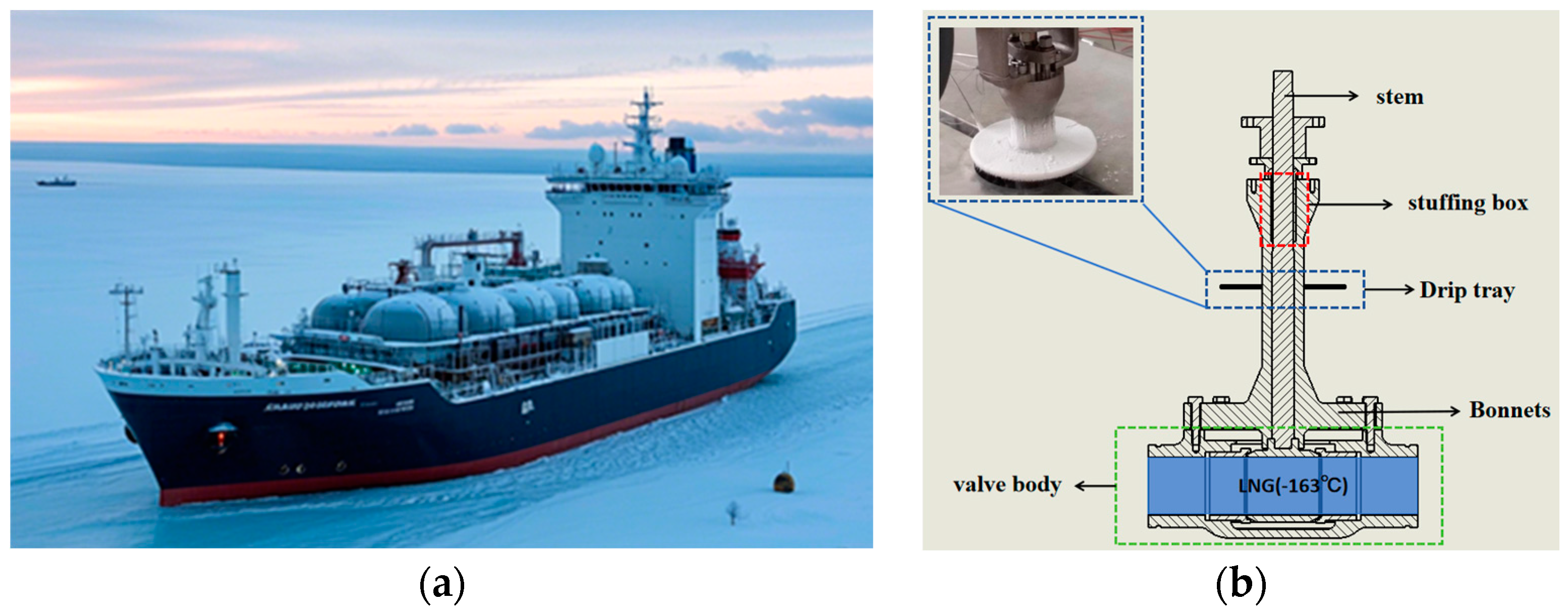
With the advancement of science and technology and global warming, the accelerated melting of sea ice in the Arctic region has led to a rise in the economic value of the region’s energy resources and shipping lanes and increased its strategic importance, which has attracted the attention of the world [1]. In this context, polar ships have received unprecedented attention. As the key basic piece of equipment for polar shipping and polar resource development, polar LNG ships provide a strong guarantee for the deployment of polar natural gas resources (as shown in Figure 1a). However, polar LNG ships face a series of complex technical challenges during operation, especially cryogenic valves, whose performance is directly related to the safety and economy of the whole polar LNG ship system. During the operation of cryogenic valves, the temperature of the air flowing through their cold surfaces decreases. When the temperature drops below the water vapour saturation point, the water vapour in the air condenses into liquid droplets, which then gather to form condensate. The condensate may enter the valve packing seals, leading to the leakage of LNG from the valve stem and packing. This reduces components’ service life and may even lead to accidents. To meet this challenge, cryogenic gate, globe, ball, and butterfly valves, as well as other UL ultra-low-temperature valves, are equipped with a drip-pan construction to increase the heat dissipation area and prevent packing failure due to low temperatures. Because drip pans are placed horizontally, condensate tends to accumulate on their surface. As condensate accumulates, the temperature of the drip-pan surface drops until it reaches or falls below the freezing point of the condensate. At this point, the accumulated water droplets begin to condense to form a frost layer and gradually thicken on the surface of the drip tray of the cryogenic valve, as shown in Figure 1b. The effect of the frost layer on the cryogenic valve can be divided into two stages, for the initial stage of frost, the existence of the frost layer makes the area of the drip tray and the air heat transfer increase. Additionally, the frost layer is unevenly distributed and the surface is rough. At this time, the frost layer plays a role similar to that of the fins, which promote heat transfer on the surface of the cryogenic valve. However, with the continuous growth of frost crystals, the thermal resistance of heat transfer on the valve surface increases, which causes the convective heat transfer capacity of the valve cover and drip-tray surface with air to be reduced, thus reducing the heat dissipation efficiency of the drip tray.

The mechanism of dew and frost is complex and not easy to control, which seriously affects the normal operation of cryogenic valves. At present, the research on cryogenic valves mainly focuses on design optimization, material selection, temperature field simulation, and other aspects. Researchers have used a variety of methods, such as analytical analysis, experimental research, and numerical simulation, to study the various components of cryogenic valves in detail. In terms of design optimization, Jin [2] simulated the temperature field of cryogenic valves by using finite element software and proposed the solution of adding an adiabatic layer to the stuffing box. Zhu [3] analyzed the temperature distribution of low-temperature valve stems and the path of cold energy transfer, and pointed out that the countermeasures to frost phenomena should be strengthened via the design, manufacturing, part installation, and maintenance of valves, etc. Veenstra [4] et al. proposed that the check valves applied to a 10 mW 4.5 K Joule Thomson refrigerated machine should be optimized for a temperature range of 50 K at an operating temperature of 50 K by investigating their operating temperature. The check valve must have an all-metal seal, and at the same time, the surface smoothness of the sealing contact surface should reach 100 μm. In terms of material selection and numerical simulation, Gao [5] conducted a temperature field analysis of DN50 ultra-low-temperature ball valves based on Workbench, and found that an increase in the thermal conductivity of the bonnet leads to a decrease in the thermal resistance, which results in a recommendation for the selection of a material with lower thermal conductivity in order to prevent the stuffing box from freezing. Ahn [6] et al. investigated the material problem of butterfly valve sealing for LNG containers, and concluded that flexible metal sealing can provide a sufficient sealing performance for butterfly valves while meeting the special requirements of cryogenic working conditions. In addition, Kim [7] and other researchers simulated the temperature and stress distribution of ultra-low-temperature ball valves through finite element analysis and computational methods, and optimized the design of high-pressure cryogenic ball valves by means of operability and structural integrity assessment, combined with special treatments and heat treatments, aiming to achieve the goal of zero leakage.

Research into frost on cold surfaces focuses on the numerical calculation method of frost growth, the exploration of frost mechanism, and the analysis of the physical parameters of the frost layer. In terms of numerical calculation, Hu [8] used Fluent 6.3.26 software to carry out an exhaustive numerical simulation of the frost-layer formation process on flat surfaces, and the simulation yielded cloud diagrams of the frost-layer temperature field, the velocity field, and ice-phase volume fraction distribution, and the results were compared and analyzed with the existing literature data. Bai [9] et al. quantitatively analyzed the cryogenic valve drip-tray frost by combining the frost growth model with the Eulerian multiphase flow model through the secondary development of Fluent. The effects of environmental parameters, such as wind speed, ambient temperature, air humidity, and cold ground surface temperature, on the growth of the frost layer were analyzed. Cui [10,11] et al. proposed a frost growth model based on the Eulerian multiphase flow calculations, and simulated the growth of the frost layer on the surface of a horizontally cooled surface and a finned tube heat exchanger by calculating the rate of mass transfer from the water vapour to the ice phase using the nucleation theory. Kim D [12] et al. also simulated the frost-layer growth based on the Eulerian multiphase flow model to simulate the frost-layer growth, and considered the water vapour concentration gradient on the frost-layer surface as the driving force of the frost-layer growth. They simulated the average height and density of the frost layer as well as the density and wet air content of the local frost layer. In terms of the frosting mechanism and the analysis of the physical properties of the frost layer, Zhao [13] conducted a detailed analysis of the frosting mechanism of low-temperature cold surfaces, which covered the changes in the physical properties of the frost layer, the factors influencing frosting, the growth law, and the heat and mass transfer properties of the frost layer. Yang [14,15] carried out a frosting test on a flat plate surface with different air temperatures, relative humidities, incoming flow velocities, and surface temperatures, and proposed a new method for assessing the frost-layer surface heat and mass transfer in the test based on the results. Based on the results, empirical correlation equations were proposed for the surface heat transfer coefficient, mass transfer coefficient, temperature, density, and the thickness of the frost layer. Xu [16] conducted an experimental study on the frosting process of a cold wall surface using microcamera technology, observed and analyzed the frosting paths of different phases of the transition processes, and assessed the effects of low-temperature cold surfaces and water vapour partial pressure on the frosting process. Xu [17] and others carried out microscopic experimental observation of the frosting process on the horizontal copper cold surface, classified it into four types according to the shape characteristics of the initial frost crystals, and pointed out that the cold surface temperature and relative humidity of the air are the key factors determining the shape of the frost crystals.

Currently, there are few studies on the effect of frost layer on the heat transfer characteristics of cryogenic valves. In this study, the thermodynamic characteristics of cryogenic valves are addressed, the law of the temperature field variation with time is deduced, and the coupling effect of frost-layer growth on the heat transfer process is considered. In order to enhance the accuracy of the simulation, this study adopts a staged simulation strategy to divide the heat transfer process of the cryogenic valve into six stages. In each stage, we take the final temperature field of the previous stage as the initial temperature field of the next stage and couple the frost layer formed in that stage with the cryogenic valve model. Through this iterative calculation method, we simulate the growth of the frost layer on the surface of the drip tray during the heat transfer process of the cryogenic valve, and then deeply analyze the specific influence of the frost layer on the heat transfer characteristics of the cryogenic valve.

2. Mathematical Model and Theoretical Analysis of Low-Temperature Valve Frosting

2.1. Frosting Model

In the operation process, depending on the ambient temperature, the air relative humidity, the flow rate, the cold surface temperature, and other factors, the wet air saturated water vapour precipitation droplets, adhering to the cold surface of low-temperature ball vales, condense into a frost. That is to say, with the passage of time, a frost layer grows on the cold surface. When working via the comprehensive consideration of the heat and mass transfer phenomenon in the phase transition process to simulate the frost process, in order to simplify the simulation process, the following assumptions are made: (1) there are two phases of wet air and ice in the calculation area, assuming that the frost layer is composed of ice crystals and wet air has a porous structure; (2) due to the low velocity of the wet air flow and the pressure change in the flow being very small, the assumption is made that the wet air is an incompressible Newtonian fluid; (3) due to the frost and the surrounding ambient temperature difference not being large, the temperature is assumed to be relatively low; (4) due to the small difference between the frost, the surrounding ambient temperature, and the low temperature, the radiative heat transfer is neglected; (5) in order to simplify the calculation, it is assumed that the phase change process in the calculation region only includes the sublimation process in which water vapour is converted into ice, and the melting and sublimation of the frost crystals are neglected.

The cause of the phenomenon of cryogenic ball valve cold surface condensation and frost is actually the concentration of water vapour in the air and the wet air speed of the joint action of the results. Figure 2 shows the cold surface of the cryogenic ball valve frost mathematical model, the ambient temperature of T, the cold surface of the cryogenic ball valve temperature of T_d, the air flow rate of u, and the wet air water vapour mass fraction of w.

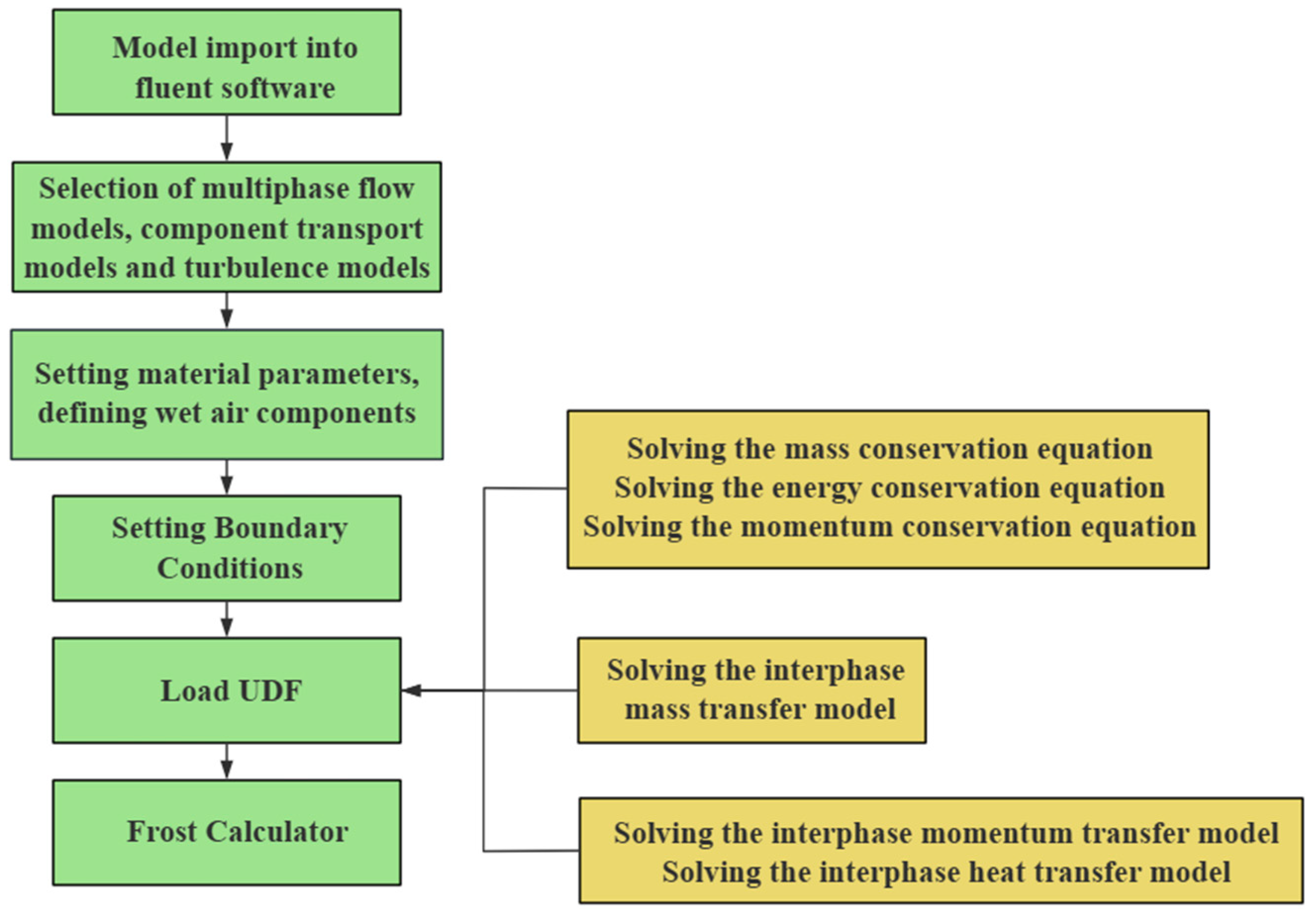
The Eulerian multiphase flow model is used to calculate the flow of the wet air phase and the ice phase and the interaction between the two phases, and the simulation of the growth of the frost-layer height and mass is achieved by assessing the mass transfer between the two phases. In the Eulerian multiphase flow model, the phases are considered as interpenetrating continua, and each phase is characterized by its volume fraction, with the sum of the volume fractions of wet air and ice being one.

$$a_a+a_i=1$$

(1)

The volume of each phase can be written as follows:

$$V={\displaystyle \underset{V}{\int }a}dV$$

(2)

2.2. Related Control Equations and Formulas

The Eulerian multiphase flow model establishes and solves the equations of the conservation of mass, momentum, and energy for each phase separately, and calculates the exchange of mass, momentum, and energy between phases. In the calculation region, the water vapour concentration in the wet air region is higher than that in the frost-layer region, and the water vapour in the wet air diffuses into the interior of the frost layer, driven by the concentration gradient. Thus, it is also necessary to establish the component conservation equations for the water vapour in the wet air. The governing equations established for the wet air phase and the ice phase are as follows:

(1)

Equation of conservation of mass

The mass conservation equation established for the wet air phase is given as follows:

$${\displaystyle \frac{\mathit{\partial }}{\mathit{\partial }t}}(a_a{\rho }_a)+\nabla \cdot (a_a{p}_a\overrightarrow{u})={\dot{m}}_{ia}-{\dot{m}}_{ai}$$

(3)

The mass conservation equation established for the ice phase is given as follows:

$${\displaystyle \frac{\mathit{\partial }}{\mathit{\partial }t}}\left(a_i{\rho }_i\right)+\nabla \cdot (a_i{p}_i{\overrightarrow{u}}_i)={\dot{m}}_{ai}-{\dot{m}}_{ia}$$

(4)

The rate of change in the mass of wet air (or ice phase) with time and space, respectively, is shown on the left side of the mass conservation equation, and the change in the mass of wet air (or ice phase) per unit of time due to a phase transition is shown on the right side. Since only the mass transfer from water vapour to ice is considered, ${\dot{m}}_{ia}=0$.

(2)

Momentum conservation equation

The momentum conservation equation established for the wet air phase is given as follows:

$${\displaystyle \frac{\mathit{\partial }}{\mathit{\partial }t}}\left(a_a{\rho }_a{\overrightarrow{u}}_a\right)+\nabla \cdot \left(a_a{\rho }_a{\overrightarrow{u}}_a{\overrightarrow{u}}_a\right)=-a_a\nabla p+\nabla \cdot {\overline{\overline{\tau }}}_a+a_a{p}_a\overrightarrow{g}+{\overrightarrow{R}}_{ia}+{\dot{m}}_{ia}{\overrightarrow{u}}_{ia}-{\dot{m}}_{ai}{\overrightarrow{u}}_{ai}$$

(5)

The momentum conservation equation established for the ice phase is given as follows:

$${\displaystyle \frac{\mathit{\partial }}{\mathit{\partial }t}}\left(a_a{\rho }_a{\overrightarrow{u}}_a\right)+\nabla \cdot \left(a_a{\rho }_a{\overrightarrow{u}}_a{\overrightarrow{u}}_a\right)=-a_i\nabla p+\nabla \cdot {\overline{\overline{\tau }}}_i+a_i{p}_i\overrightarrow{g}+{\overrightarrow{R}}_{ai}+{\dot{m}}_{ai}{\overrightarrow{u}}_{ai}-{\dot{m}}_{ia}{\overrightarrow{u}}_{ia}$$

(6)

The left-hand side of the momentum equation shows the change in momentum of the wet air phase (or ice phase) with time and space $a_a{p}_a\overrightarrow{g}$. The effect of gravity on the momentum of the wet air is determined: $\overrightarrow{g}$ is the gravitational acceleration; ${\overrightarrow{R}}_{ia}$ is the trailing effect of the ice phase on the wet air phase; ${\dot{m}}_{ia}{\overrightarrow{u}}_{ia}$ and ${\dot{m}}_{ai}{\overrightarrow{u}}_{ai}$ are the changes in momentum between the wet air and ice phases due to the exchange in mass; and ${\overrightarrow{u}}_{ia}$ and ${\overrightarrow{u}}_{ai}$ stand for the velocity of the phases, respectively. In Equation (5), ${\dot{m}}_{ia}=0;{\dot{m}}_{ci}>0,{\overrightarrow{u}}_{ci}={\overrightarrow{u}}_a$. Since the wet air is a Newtonian fluid, according to the generalized Newton’s law, the stress tensor ${\overline{\overline{\tau }}}_a$ of the wet air can be written as a linear equation for the strain rate tensor of the fluid:

$${\overline{\overline{\tau }}}_a=a_a{p}_a{v}_a(\nabla {\overrightarrow{u}}_a+\nabla {{\overrightarrow{u}}_a}^T)-a_a(p+{\displaystyle \frac{2}{3}}{p}_a{v}_a\nabla \cdot \overrightarrow{u})\overline{\overline{I}}$$

(7)

where $\nabla {\overrightarrow{u}}_a$ is the strain rate tensor of the wet air; v_a is the kinematic viscosity coefficient of the wet air; and $\overline{\overline{I}}$ is the unit second order tensor.

(3)

Energy conservation equation

The energy conservation equation is established for the wet air phase as follows:

$${\displaystyle \frac{\mathit{\partial }}{\mathit{\partial }t}}\left(a_a{\rho }_a{h}_a\right)+\nabla \cdot \left(a_a{\rho }_a{\overrightarrow{u}}_a{h}_a\right)=q_{ia}+a_a{\displaystyle \frac{\mathit{\partial }{p}_a}{\mathit{\partial }t}}+{\overline{\overline{\tau }}}_a:\nabla {\overrightarrow{u}}_a+{\dot{m}}_{ia}{h}_{ia}-{\dot{m}}_{ai}{h}_{ai}$$

(8)

The energy conservation equation is established for the ice phase as follows:

$${\displaystyle \frac{\mathit{\partial }}{\mathit{\partial }t}}\left(a_i{\rho }_i{h}_i\right)+\nabla \cdot \left(a_i{\rho }_i{\overrightarrow{u}}_i{h}_i\right)=q_{\mathit{ai}}+a_i{\displaystyle \frac{\mathit{\partial }{p}_i}{\mathit{\partial }t}}+{\overline{\overline{\tau }}}_i:\nabla {\overrightarrow{u}}_i+{\dot{m}}_{ai}{h}_{ai}-{\dot{m}}_{ia}{h}_{\mathit{ia}}$$

(9)

In the energy conservation equation, the left side of the equation is the rate of change in enthalpy per unit volume of wet air phase (or ice phase) with time and space; h_a and h_i are the enthalpies of wet air and ice, respectively; q_ia and q_ai are the rates of heat exchange between the phases per unit volume; ${\overline{\overline{\tau }}}_a:\nabla {\overrightarrow{u}}_a$ and ${\overline{\overline{\tau }}}_i:\nabla {\overrightarrow{u}}_i$ include the work carried out by overcoming the normal force of traction and overcoming the viscous force of the fluid as it expands; and ${\dot{m}}_{ai}{h}_{ai}$ and ${\dot{m}}_{ia}{h}_{ia}$ are the changes in energy due to the mass exchanges between the wet air and ice phase.

(4)

Component conservation equations

The component conservation equation is established for water vapour in wet air as follows:

$${\displaystyle \frac{\mathit{\partial }}{\mathit{\partial }\mathrm{t}}}(a_a{p}_a{w}_v)+\nabla \cdot (a_a{p}_a{w}_a{\overrightarrow{u}}_a)=\nabla \cdot (p_a{D}_{va}\nabla w_v)$$

(10)

In the component conservation equations, the left-hand side of the equation is the rate of change in water vapour concentration with time and space; w_v is the mass fraction of water vapour in the wet air; $\nabla \cdot (p_a{D}_{\nu a}\nabla w_{\nu })$ is the change in concentration due to diffusion of water vapour; and D_va is the diffusion coefficient of water vapour in the wet air.

In the above control equations, in contrast to the control equations for single-phase flow, the calculations need to give the mass transfer between phases and also include the transfer of momentum and energy due to the mass transfer between phases.

(5)

The phase transition rate is calculated as follows:

$$m_{\mathrm{phase} }={\displaystyle \frac{\left(\rho D/{\delta }_d\right)}{\rho D/\delta +C_{\mathrm{phase} }}}{C}_{\mathrm{phase} }\left(y_s-y_i\right)$$

(11)

m_phase is the molar mass of the vapour component and the mixture, g/mol; ρ is the density of the gas mixture, kg/m³; D is the mass diffusivity of the vapour component, m²/s; y_i is the mass fraction of the vapour component in the centre of the cell; and δ_d the distance from the centre of the cell to the wall, m.

(6)

The saturated mass fraction is calculated using the following formula:

$${\phi }_s={\displaystyle \frac{w_{\mathrm{s}}(T)}{1+w_{\mathrm{s}}(T)}}$$

(12)

$$w_{\mathrm{s}}(T)=0.62198{\displaystyle \frac{P_{\mathrm{s}}(T)}{P_0-P_{\mathrm{s}}(T)}}$$

(13)

W_s(T) is the saturated wet air content; P_s(T) is the absolute mixture pressure; and P₀ is the atmospheric pressure, where P₀ = 1.01325 × 10⁵ pa.

(7)

The formula for calculating the saturated water vapour pressure is as follows [8]:

When 173.15 k ≤ T ≤ 273.15 k, the

$${\mathrm{P}}_s(T)=\exp \left({\displaystyle \frac{{\mathrm{a}}_0}{T}}+{\mathrm{a}}_1+{\mathrm{a}}_{2}T+{\mathrm{a}}_3{T}^2+{\mathrm{a}}_4{T}^3+{\mathrm{a}}_5{T}^4+{\mathrm{a}}_6\ln T\right)$$

(14)

When T > 273.15 k, the

$$P_s( T)=\exp \left({\displaystyle \frac{b_0}{T}}+b_1+b_{2}T+b_3{T}^2+b_4{T}^3+b_5\ln T\right)$$

(15)

The coefficients are as follows: a₀ = −5.6745359 × 10³, a₁ = 6.3925247, a₂ = −9.677843 × 10⁻³, a₃ = 6.22157 × 10⁻⁷, a₄ = 2.0747825 × 10⁻⁹, a₅ = −9.484024 × 10⁻¹³, a₆ = 4.1635019, b₀ = −5.8002206 × 10³, b₁ = 1.3914993, b₂ = −4.8640239 × 10⁻², b₃ = −4.1764768 × 10⁻⁵, b₄ = −1.4452093 × 10⁻⁸, and b₅ = 6.5459673.

3. Numerical Methods and Frost Calculations

3.1. Numerical Simulation Methods

In this study, the two-dimensional numerical simulation of the surface frosting process of the drip tray of cryogenic ball valve is carried out based on Fluent, and DesignModeler is used to build the model and divide the mesh. After importing Fluent, using Transient mode, we select the component transport model, the Eulerian multiphase flow model, and the turbulence model (laminar flow); open the energy equation; define the material parameters; set the ice-phase parameters; and define the components of multiphase wet air—water, oxygen, and nitrogen. Then, we set the boundary conditions. Specifically, we set the inlet velocity, air relative humidity, cold edge temperature, and ambient temperature; import the UDF for frost growth calculation; and obtain the thickness of the frost and the volume fraction of ice phase by solving the equations of momentum conservation, mass conservation, energy conservation, component conservation, and mass fraction conservation. A flowchart of the numerical simulation of frosting on the drip tray of the low-temperature valve is shown in Figure 3.

3.2. Physical Modelling and Parameter Setting

The flow field domain on the upper surface of the drip tray is simplified as a 2D planar model with a length of 75 mm. The inlet height of the wet air is 5 mm, the left side of the model is the inlet of the wet air, and the right side is the outlet of the wet air. The upper side is the adiabatic wall, and the lower side is the cold wall (the upper surface of the drip tray), as shown in Figure 4 [18].

In this paper, the geometric structure of the computational object is simple, and a rectangular grid of equal size is used. After the verification of grid independence, the size of the grid cells in the x- and y-directions are taken as Δx = 0.1 mm and Δy = 0.05 mm, respectively, and the finite element model after meshing is shown in Figure 5.

A Eulerian multiphase flow model is used in the numerical calculations, and two phases, the wet air phase and the ice phase, are set up with the physical parameters shown in

Table 1. Physical parameters of wet air and ice.

Materialistic	Densities kg/m3	Heat Conductivity W/(m·k)	Specific Heat Capacity J/(kg·k)	Coefficient of Viscosity Kg/(m·s)
Dry air	1.225	-	-	1.75 × 10−5
Water vapour	0.554	-	-	1.34 × 10−5
Humid air	quality-weighted	0.024	1006.4	quality-weighted
Ice	915	2.5	2100	-

. The wet air includes the components of dry air and water vapour, the mass fraction of the wet air components is set in the wet air inlet conditions, and the inter-phase mass transfer and inter-phase forces are added to the calculations by custom functions.

3.3. Validation of Frosting Model

In order to verify the accuracy of the numerical simulation method, this study conducted numerical simulations based on the experimental conditions set by Ma et al. [19]. The simulation parameters were set as follows: an ambient temperature of 2 °C, a wet air velocity of 0.92 m/s, a cold wall surface temperature of −13 °C, and an air relative humidity of 85%. Figure 6 shows the frosting of the numerical simulation and the experiment under the same working conditions at different times.

It can be observed that the trend in the development of the frost layer with time in the numerical simulation is more in line with the experimental observations. Both the frost-layer height and volume fraction increase with time. In order to accurately determine the results in the comparative literature, the average height of the frost layer obtained from the simulation is analyzed in comparison with the results of the average height of the frost layer obtained from the literature experiments, as shown in Figure 7.

The average height of the frost layer derived from the simulation was compared with the experimental results to analyze the error of the average height of the frost layer obtained from the numerical simulation and the experiment under different frosting times, and the comparison of the error is shown in

Table 2. A comparison of the errors between the numerical and experimental results.

Time (min)	10	20	30	40	50
Numerical results (mm)	0.54	0.96	1.32	1.62	1.92
Experimental results (mm)	0.49	0.88	1.22	1.53	1.82
Relative error (%)	10.2	9.0	8.8	5.8	5.5

.

As can be seen from Table 2, under the same working conditions, the numerical simulation results obtained from the frost-layer growth model used in this paper have a maximum error of 10.2% in relation to the literature test results, while the frost-layer growth morphology is also very similar. As such, the average frost-layer height and ice-phase volume fraction calculated in this paper are within the error tolerance, which verifies the accuracy of the numerical simulation method used.

3.4. Calculation of Frost-Layer Height

In this study, the research object is the cryogenic valve on a polar LNG ship, and the climatic conditions of polar summer navigation are selected: we chose a wet air flow rate of 1 m/s, an air humidity of 85%, and an ambient temperature of 2 °C as the boundary conditions for numerical simulation. Through the transient thermal numerical simulation of the cryogenic ball valve without considering the effect of the frost layer, it is found that, at an ambient temperature of 2 °C, the average temperature of the drip tray gradually decreases with the conduction of the cold temperature at the bottom and tends to stabilize after 3500 s, and the stabilized temperature is 21.5 °C, as shown in Figure 8a. Therefore, this study used the slicing method to divide the wall temperature change into six stages—2~−2 °C, −2~−6 °C, −6~−10 °C, −10~−14 °C, −14~−18 °C, and −18~−21.5 °C—and used the initial temperature of each stage as the wall temperature of the stage for the calculation of frost. In this case, there is no frost growth in the first stage when the wall surface temperature is 2 °C, and so only five stages are accompanied by frost growth. Frosting calculations are performed for the corresponding durations using the wall surface temperature of each stage, respectively, so as to obtain the growth of the frost layer at different time stages and the overall height of the frost layer at the corresponding frosting time, as shown in Figure 8b and

Table 3. The growth of the frost layer at each stage and the height of frost layer at the corresponding time.

Wall Temperture (°C)	2	−2	−6	−10	−14	−18
Stage frosting Time (s)	587	334	376	480	735	988
Stage frost Height (mm)	0	0.21	0.31	0.49	0.93	1.51
Frosting time (s)	587	921	1297	1777	2512	3500
Frost height (mm)	0	0.21	0.52	1.01	1.94	3.45

.

4. Low-Temperature Valve Heat Transfer Model and Heat Transfer Calculation

In the practical application of cryogenic valves, the temperatures of their components are dynamically adjusted with the change in time and finally reach a stable state, and this process belongs to unsteady-state heat transfer. This paper focuses on the two-dimensional unsteady-state heat conduction problem of the long-necked bonnet and drip tray of cryogenic valves with constant physical properties, no internal heat source, and non-chiral boundary conditions. Then, it constructs a mathematical model of heat transfer through reasonable assumptions and model simplification, numerically analyses the transient temperature field of the overall valve by using the differential equations of heat conduction and boundary conditions, and applies the method of solving the equations of mathematical physics to reveal the law of the change in its temperature field with time. In engineering practice, the heat transfer mode of low-temperature valve operation is mainly based on heat conduction and convection heat transfer. As shown in Figure 9, the low-temperature valve heat transfer process is as follows: due to heat conduction and convective heat transfer, the low-temperature medium is cold to the valve body wall; the valve body becomes cold through heat conduction along the valve cavity to the long-necked bonnet; energy is transferred to the long-necked bonnet’s cold wall and then transferred to the long-necked bonnet’s wall of the bonnet through heat conduction; it is then transferred to the wall of the bonnet, the drip tray, and the surrounding environment via heat conduction and convective heat transfer.

4.1. Analysis of Low-Temperature Valve Heat Transfer Methods

The numerical simulation of the transient temperature field of the cryogenic valve is carried out using finite element analysis, and the process of the surface temperature change of the cryogenic valve with time is observed by analyzing the results of the numerical simulation in order to grasp the heat transfer characteristics of the cryogenic valve. The main control equations of the numerical simulation of the temperature field of the cryogenic valve are outlined below.

(1)

Equation of conservation of mass

The law of the conservation of mass states that the rate of increase in the mass of the control body is equal to the difference between the inflow mass and the outflow mass. The mathematical description of the continuity equation is as follows:

$${\displaystyle \frac{\mathit{\partial }\rho }{\mathit{\partial }\tau }}+{\displaystyle \frac{\mathit{\partial }(\rho u_x)}{\mathit{\partial }x}}+{\displaystyle \frac{\mathit{\partial }(p{v}_y)}{\mathit{\partial }y}}+{\displaystyle \frac{\mathit{\partial }(\rho {\omega }_z)}{\mathit{\partial }z}}=0$$

(16)

where ρ is the density of the control body, kg/m²; τ is the time, s; and u_x, v_y, and w_z are the components of the velocity in the x, y, and z directions, m/s, respectively.

(2)

Momentum conservation equation

The law of the conservation of momentum states that when the rate of change in momentum inside the microelement plus the net rate of flow of momentum out of the microelement within the control body is equal to the total rate of change in momentum, the equation of conservation of momentum needs to be derived on the basis of conservation of mass, and its mathematical representation is as follows:

$$\rho {\displaystyle \frac{Du}{D\tau }}={\displaystyle \frac{\mathit{\partial }{p}_x}{\mathit{\partial }x}}+{\displaystyle \frac{\mathit{\partial }{p}_y}{{\mathit{\partial }}_y}}+{\displaystyle \frac{\mathit{\partial }{p}_z}{\mathit{\partial }z}}+\rho f$$

(17)

where f is the unit mass, m/s².

(3)

Energy conservation equation

The law of conservation of energy is expressed as the sum of the heat transferred by a system from the outside world and the work performed on it by an external force is equal to the amount of change in the internal energy of the system. The continuity equation that describes this mathematically is as follows:

$$\rho {\displaystyle \frac{D}{D\tau }}\left(E+{\displaystyle \frac{1}{2}}u\cdot u\right)=\mathit{\nabla }(\Sigma u)+\rho u\cdot f-\mathit{\nabla }\cdot Q$$

(18)

where E is kinetic energy and Q is thermal energy in J.

For different engineering problems, the above three equations are discretized separately as needed. For the numerical simulation of the temperature field, the energy conservation equation is usually solved. The finite element thermal analysis of the temperature field of an object is based on Fourier’s law and is used to study the thermal response of the object under thermal loading. The thermal equilibrium matrix is as follows:

$$[C(T)]\left\{\dot{T}\right\}+[K(T)]\left\{T\right\}=[Q(T)]$$

(19)

where $\left[C\right]$ is the heat capacity matrix; $\left\{\dot{T}\right\}$ is the temperature matrix; $\left[K\right]$ is the heat conduction matrix; and $\left\{Q\right\}$ is the heat flow rate loading.

Transient heat transfer is a process in which the temperature, thermal boundary conditions, and heat flow rate in the system all change with time. Its heat balance equation is as follows:

$$[C]\left\{\dot{T}\right\}+[K]\left\{T\right\}=\left\{Q\right\}$$

(20)

where $\left[K\right]$ is the conduction matrix, including thermal conductivity, convective heat transfer coefficient, etc.; $\left[C\right]$ is the specific heat matrix; $\left\{\dot{T}\right\}$ is the derivative of temperature with respect to time; $\left\{T\right\}$ is the nodal temperature; and $\left\{Q\right\}$ is the nodal heat flow rate.

When a system is at thermal steady state, the sum of the heat generated by the system itself and the heat flowing into the system equals the heat flowing out of the system. The energy equation for steady state thermal analysis is as follows:

$$[K](T)=\left\{Q\right\}$$

(21)

4.2. Modelling and Boundary Condition Setting

4.2.1. Cryogenic Ball Valve Modelling

In this study, a finite element analysis model of cryogenic ball valve frosting is constructed, and the distance between the lower face of the bonnet flange and the bottom of the stuffing box is L₁ = 0.52 m. The distance from the bottom of the stuffing box to the top of the valve stem is L₂ = 0.27 m, the inner diameter of the drip tray is r₁ = 0.0645 m, and the outer diameter of the drip tray is r₂ = 0.1395 m. Due to the horizontal placing of the drip tray, the condensate easily accumulates on the surface of the drip tray. As the condensate accumulates and the temperature on the surface of the drip tray decreases, the accumulated water droplets begin to condense and form a frost layer, which gradually thickens on the surface of the drip tray of the low-temperature ball valve. Therefore, the frost layer was coupled to the upper surface of the drip tray in the manner shown in Figure 10a. The construction of the three-dimensional model of the cryogenic ball valve was completed using SpaceClaim 2021 R1 software. Then, the model was meshed in ANSYS Workbench 2021R1 software and the temperature field was solved numerically. After meshing, the obtained finite element model contained 166,313 nodes and 89,229 cells. The detailed geometry and meshing results of the model are shown in Figure 10b.

4.2.2. Boundary Condition Settings for Heat Transfer Calculation

(1)

Boundary condition settings for the numerical calculation of the temperature field of cryogenic valves:

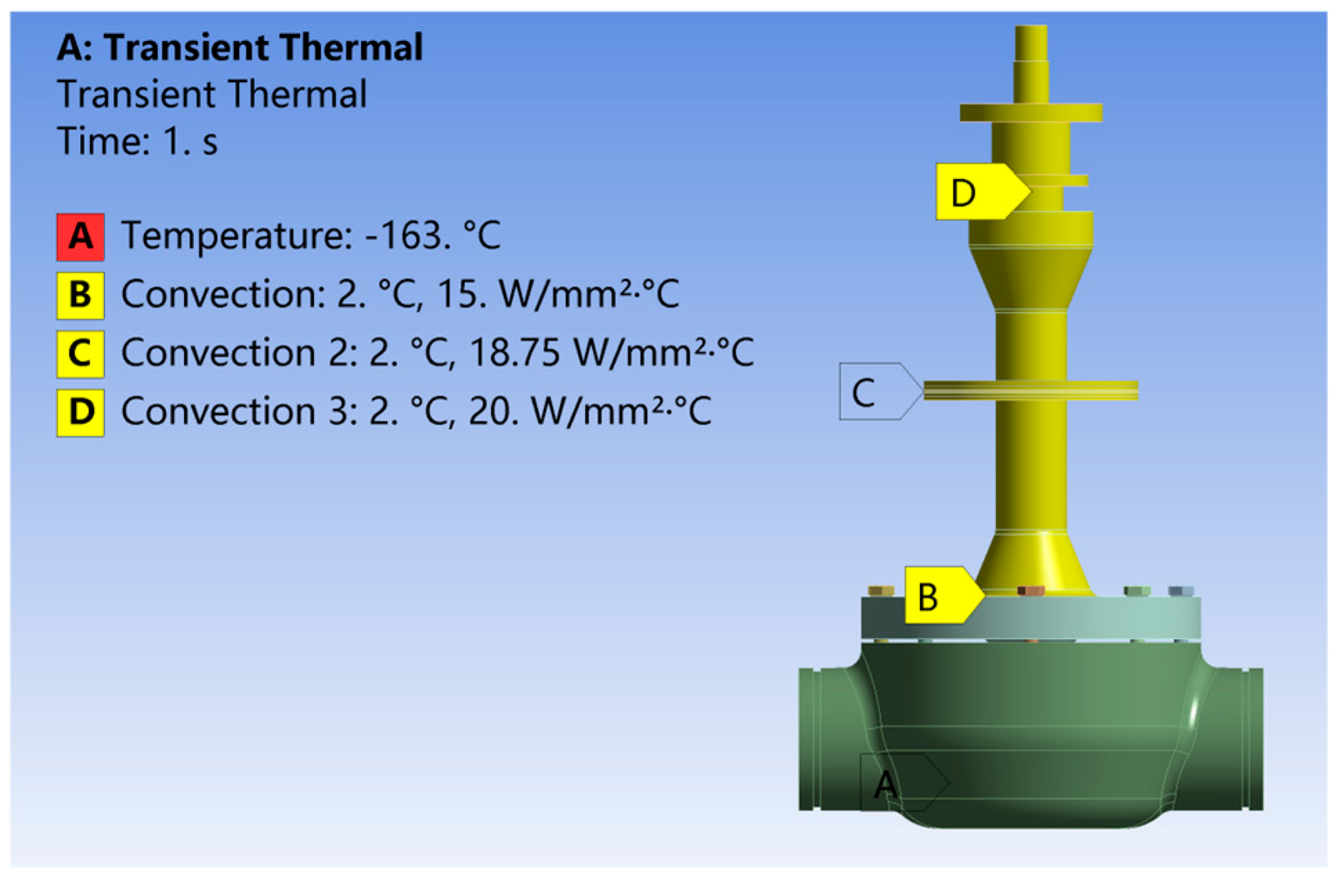
The material used in this study for the cryogenic ball valves was ASTM A351 CF3M manufactured by Jiaxing Maxtor Stainless Steel Co. Ltd. in Jiaxing, China, with a thermal conductivity of 12.3 W/(m²·K). The ambient temperature is set to 2 °C, assuming that its physical parameters do not change with the temperature, the bonnet neck wall surface, the drip-tray outer wall surface, and the space for natural convection heat transfer, the natural convection heat transfer coefficient is set to 15 W/(m²·K), the stem portion of the valve above the stuffing box and the natural convection heat transfer coefficient of the air is set to 20 W/(m²·K), and the temperature of the bonnet flange lower end face, the valve seat, and the valve body inner wall is set to −163 °C.

(2)

Boundary condition setting for numerical calculation of frost-layer temperature field:

It has been shown that the thermal conductivity of the frost layer mainly depends on density, but it also depends on the microstructure of the frost layer, which is the result of the interaction between the structure of the frost layer, the water vapour diffusion caused by the temperature gradient within the frost layer and the release of the latent heat of condensation, and the eddy current effect caused by the roughness of the frost surface. At present, the most widely used method of determination is the correlation equation of thermal conductivity proposed by Yonko and Sep sy [20]. In terms of convective heat transfer coefficient, due to the increase in the roughness of the rib surface after frost, the apparent heat transfer coefficient increases and, in general, the heat transfer coefficient between the air and the frost layer is 1.2–1.3 times that of the heat transfer coefficient of the heat exchanger’s outer surface when it is not frosted.

The formulae for calculating the physical parameters of the frost layer [20,21] are as follows:

$${\rho }_{fr}=340{\left|{\mathrm{T}}_{fr}\right|}^{0.455}+25u_f$$

(22)

$$\lambda =0.02422+7.214\times {10}^{-4}{\rho }_{fr}+1.1797\times {10}^{-6}{{\rho }_{fr}}^2$$

(23)

$${\alpha }_{af}=(1.2-1.3){\alpha }_w$$

(24)

where ${\rho }_{fr}$—density, kg/m³; $T_{\mathit{fr}}$—the surface temperature of the frost layer; °C. $u_f$—wind speed, m/s; ${\alpha }_w$—the heat transfer coefficient of the outer surface of the fins when they are not frosted, W/(m²·K); ${\alpha }_{\mathit{af}}$—the heat transfer coefficient of the convection heat transfer of the frost layer, W/(m²·K).

The density of frost = 0.491 g/cm³, thermal conductivity = 0.662 W/(m·k), and convective heat transfer coefficient = 18.75 W/(m²·K). These values are calculated using the above equations, and it is assumed that the physical parameters of the frost layer do not change with temperature. Figure 11 demonstrates the overall boundary condition set-up for the coupled frost-layer valve.

4.3. Validation of Numerical Methods

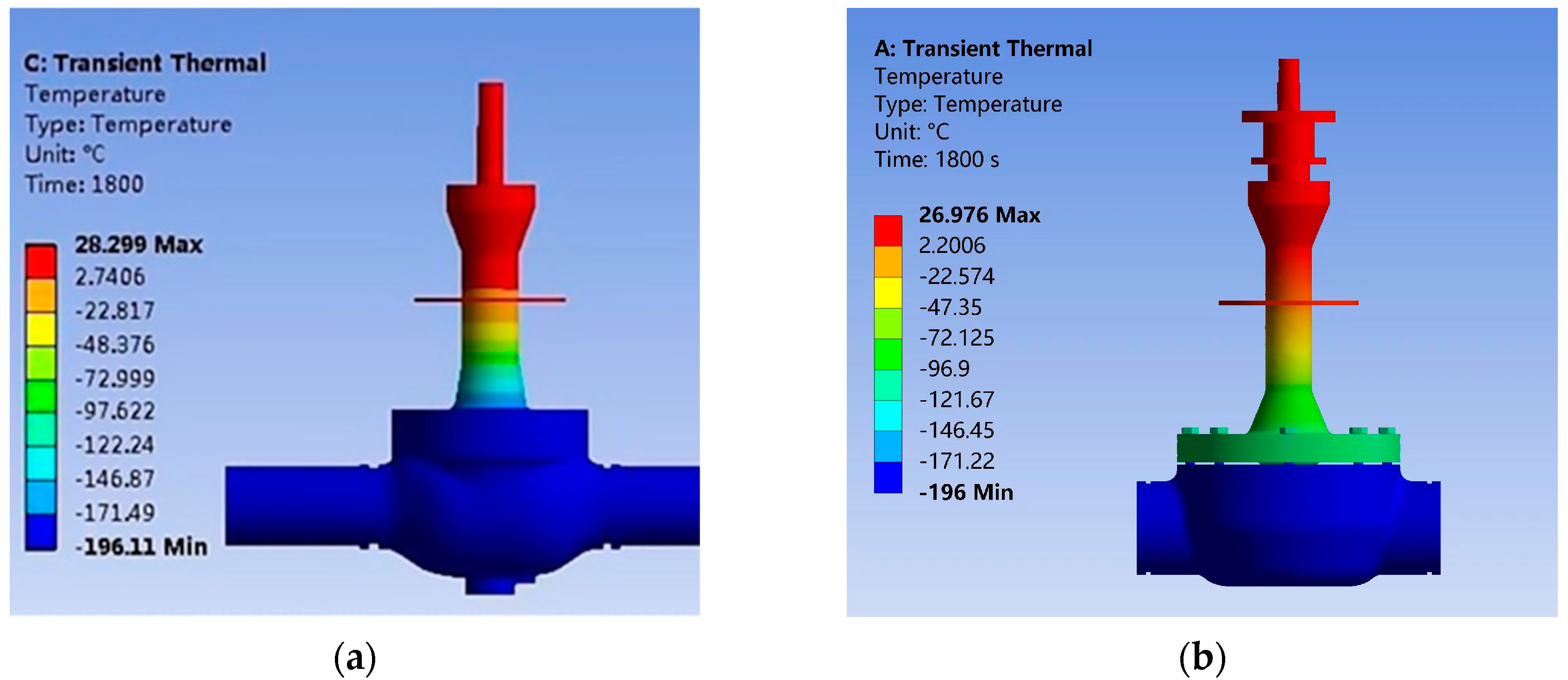
In order to verify the accuracy of the numerical simulation method, this study solves the transient temperature field of the cryogenic ball valve using ANSYS Workbench software, and the temperature field distribution of the cryogenic ball valve after 1800 s is obtained by setting the coefficient of natural convective heat transfer as well as the temperature parameter, as shown in

Table 4. Calculation of working condition parameters for cryogenic ball valves.

Environmental Temperature	Convective Heat Transfer Coefficient		Thermal Conductivity	Low Temperature Medium Temperature
°C	W/(m2·K)		W/(m·K)	°C
Tair	h1	h2	λ	TLNG
30	15	20	12.3	−196

. The results are compared and verified with those of Jia et al. [22], as shown in Figure 12a,b.

As can be seen from Figure 12, the temperature field distribution of the simulation results in this paper matches very well with the simulation results of Jia et al. under the same working conditions. The lowest value of the temperature field distribution in the simulation results of this paper is −196 °C, and the highest value is 26.976 °C; the lowest value of the temperature field distribution in the simulation of Jia is −196.11 °C, and the highest value is 28.299 °C. The relative error between the lowest temperature in the simulation results of this paper and those in the literature is only 0.056%, and the relative error of the highest temperature is only 4.67%, and so the numerical simulation method used in this paper is considered to be feasible.

4.4. Study on the Effect of Frost Layer on Heat Transfer in Cryogenic Valves

The aim of this study is to investigate the effect of the frost layer on the heat transfer characteristics of cryogenic valves. This study used the Workbench transient thermal module for heat transfer analysis and divided the whole heat transfer process into six stages: 2 °C to −2 °C, −2 °C to −6 °C, −6 °C to −10 °C, −10 °C to −14 °C, −14 °C to −18 °C, and −18 °C to −21.5 °C. In each heat transfer stage, the final temperature field of the previous stage was used as the initial temperature field of the next stage, and the frost layer formed in that stage was coupled with the valve model of the previous stage before heat transfer calculations were performed in this stage. In order to accurately evaluate the effect of the frost layer on the heat transfer mechanism, we first performed numerical simulations of the valve under frost-free-layer conditions. By comparing the simulation results of the temperature field of the valve under the frost-free-layer and the coupled frost-layer conditions, we analyzed the specific influence of frost-layer growth on the heat transfer characteristics of the cryogenic valve, so as to provide a theoretical basis and technical support for optimizing the design of cryogenic valves and their heat transfer performance.

4.4.1. Comparative Analysis of the Temperature Field of Cryogenic Valves With and Without a Frost Layer

In order to investigate the effect of the frost layer on the heat transfer performance of the low-temperature valve, the temperature field distribution of the valve at each moment in time, with and without the presence of the frost layer, was calculated by numerical simulation in this study, as shown in Figure 13 and Figure 14. In addition, Figure 15a compares the maximum temperature of the valve with and without the presence of a frost layer, while Figure 15b demonstrates the trend in the temperature difference over time caused by the presence of a frost layer.

By visualizing the heat transfer process, it can be observed that the cold temperature is gradually conducted from the bottom to the top of the valve with the passage of time, forming an obvious gradient of temperature distribution with a gradual increase in temperature from the bottom to the top. In particular, the drip tray, serving as the dividing line, is designed to increase the heat dissipation area and thus improve the heat dissipation efficiency. As a result, a significant decrease in the temperature gradient of the upper structure can be clearly seen as the cold temperature passes through the drip tray. In terms of the effect of the frost layer on the heat transfer characteristics of the valve, it can be seen from Figure 15a,b that the maximum temperature (the temperature at the top of the valve stem) is basically the same for both the valves with and without the frost layer before 921 s. At this time, the height of the frost layer is only 1.01 mm, which is not sufficient to have an effect on the maximum temperature of the valve. However, with the continuous growth of the frost layer on the surface of the drip tray, the convective heat transfer capacity is gradually enhanced. The maximum temperature of the valve during the period from 921 s to 1297 s began to gradually show the impact of the frost layer. At this time, the height of the frost layer was 0.52 mm. Using the bottom of the cold temperature conduction area and the frost layer of the continuous growth to assess the difference between the maximum temperature of the valve with and without a frost layer, we saw a small but stable upward trend, and at 3500 s, this temperature difference reached the maximum value in the observation process, which was 0.165 °C, at which time the frost-layer height increased to 3.45 mm. Obviously, the influence of the frost layer on the heat transfer characteristics of the valve is mainly concentrated in the region between the drip tray and the stuffing box in the 3500 s time span, while the influence on the overall maximum temperature of the valve is relatively small. Therefore, this study focuses on the temperature distribution changes in the valve drip pan and stuffing box when coupled with the frost layer, aiming to reveal the influence of the frost layer on the heat transfer mechanism of the valve.

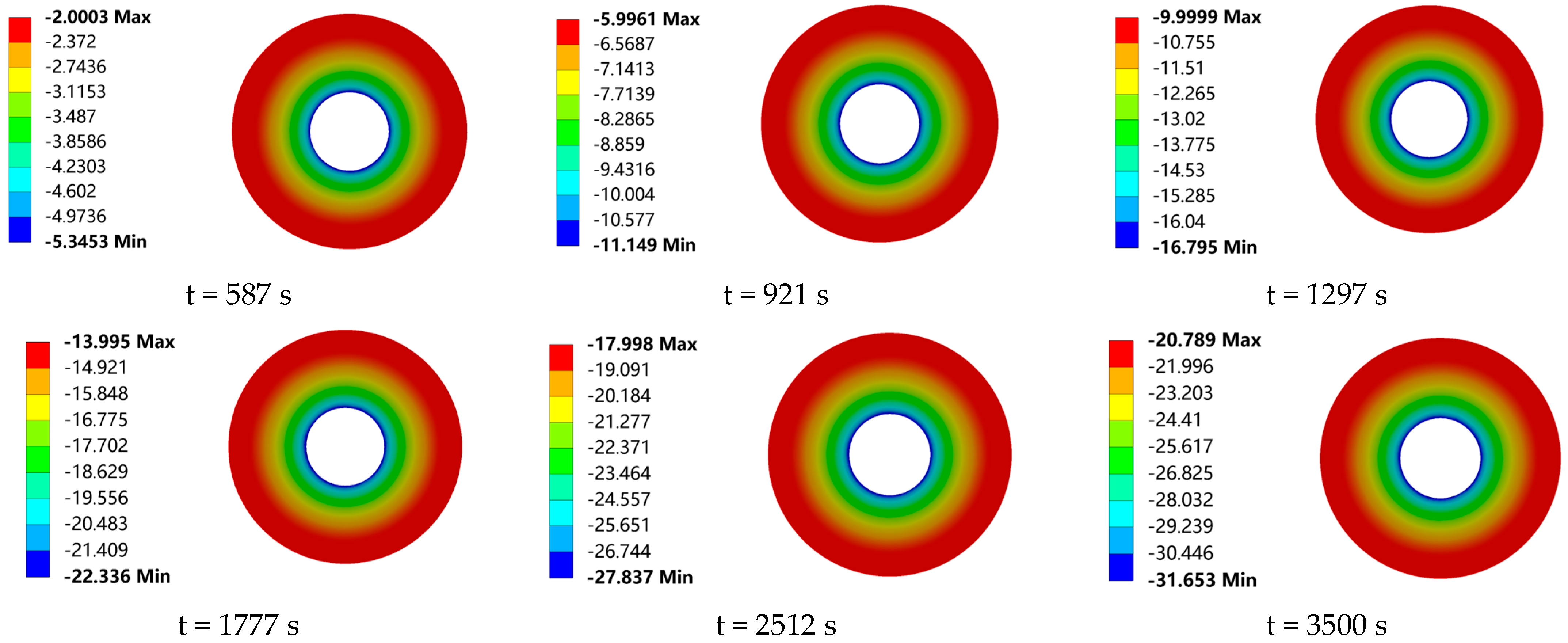
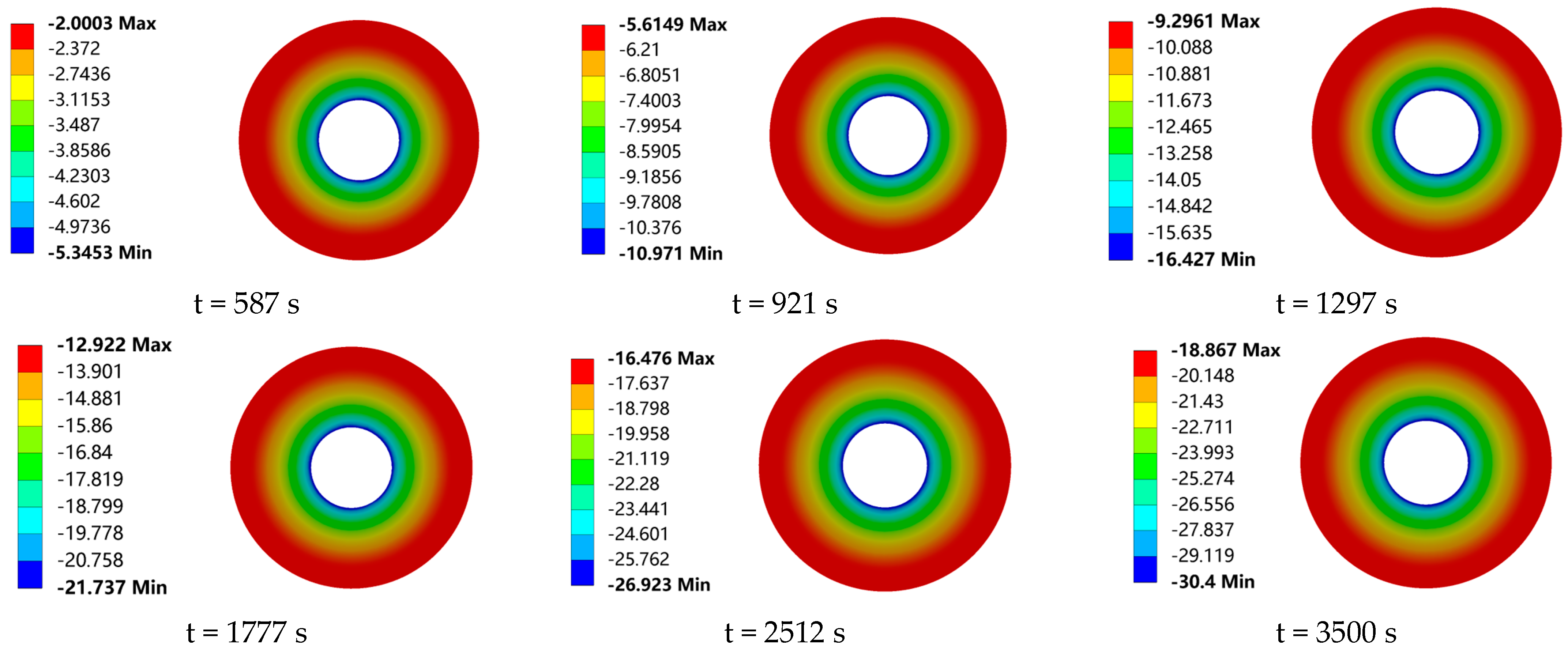
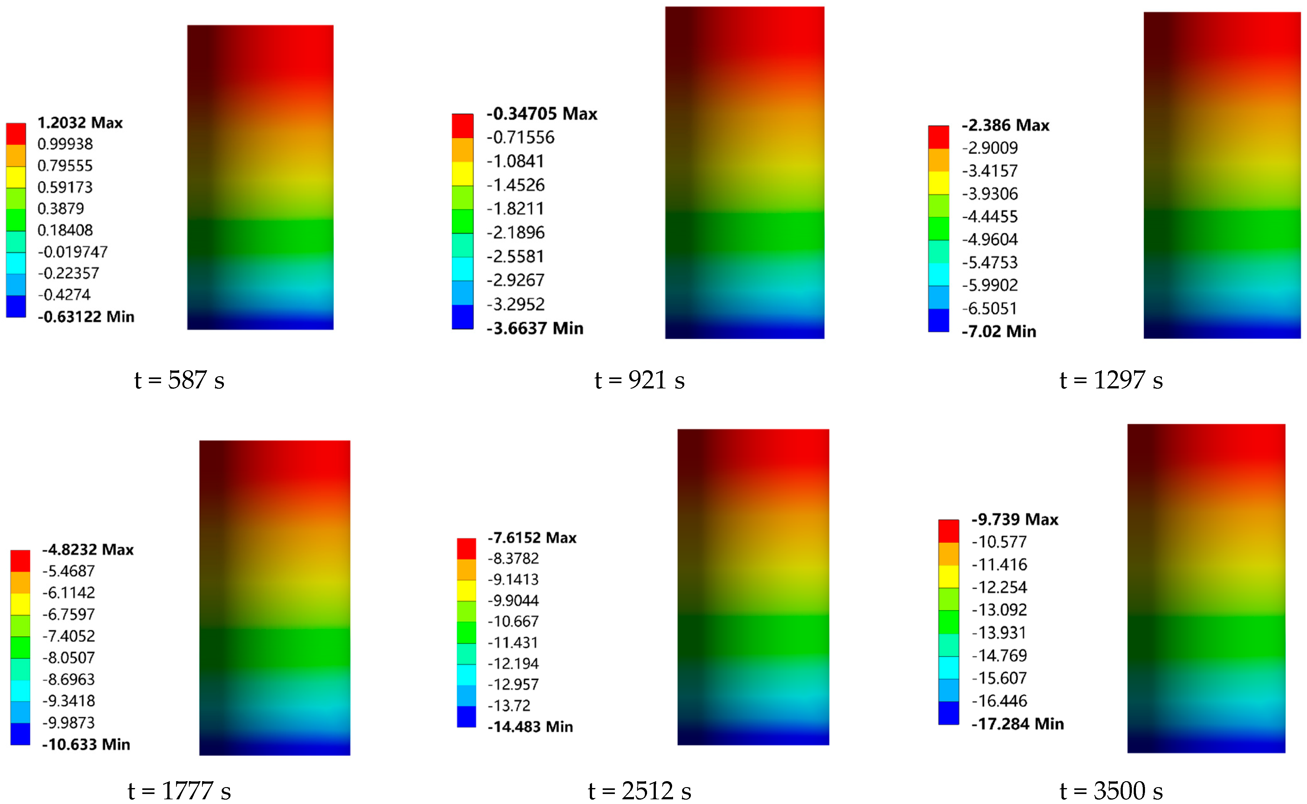
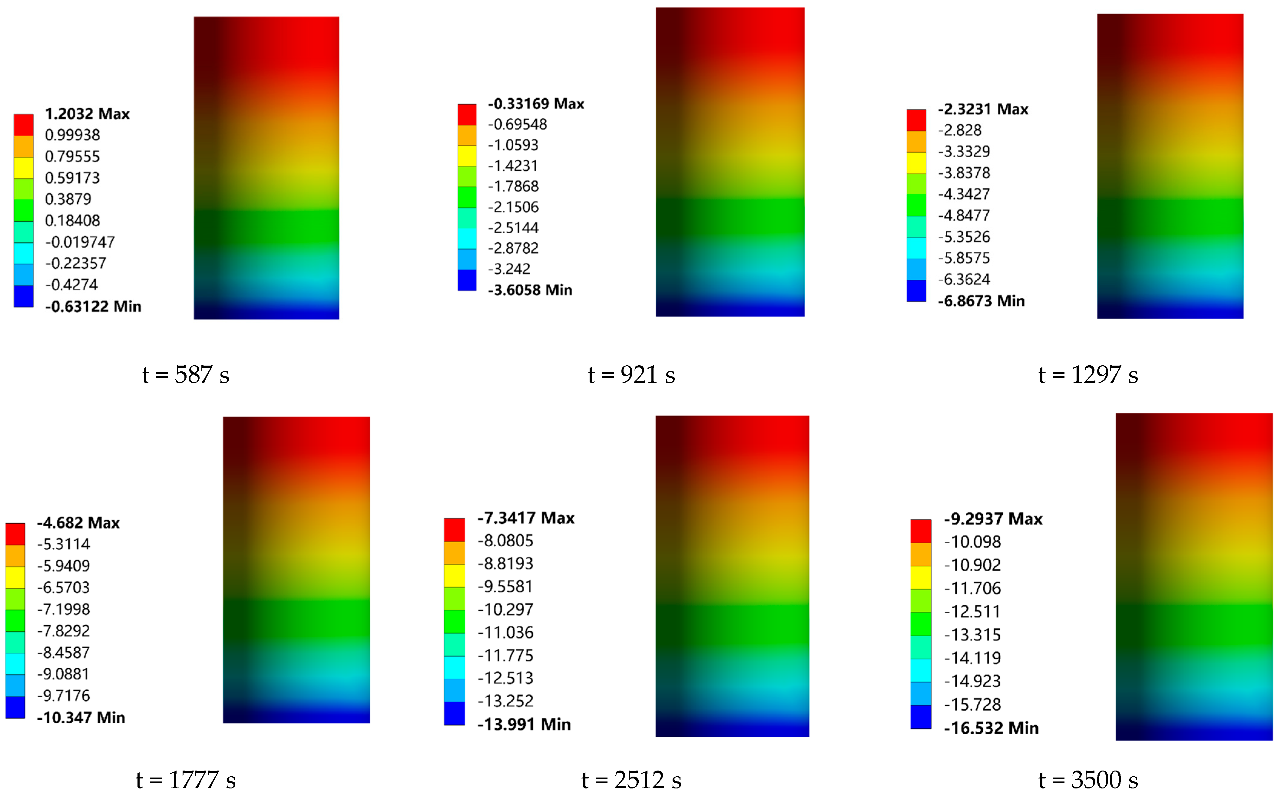
4.4.2. Comparative Analysis of Temperature Field of Drip Tray With and Without Frost Layer

The valve drip-tray structure is designed to increase the heat dissipation area in order to avoid packing failure due to low temperatures. In this study, in order to investigate the effect of the frost layer on the heat transfer of the drip-tray structure, the temperature field distribution of the drip tray was calculated, in the presence or absence of a frost layer, by numerical simulation, as shown in Figure 16 and Figure 17. 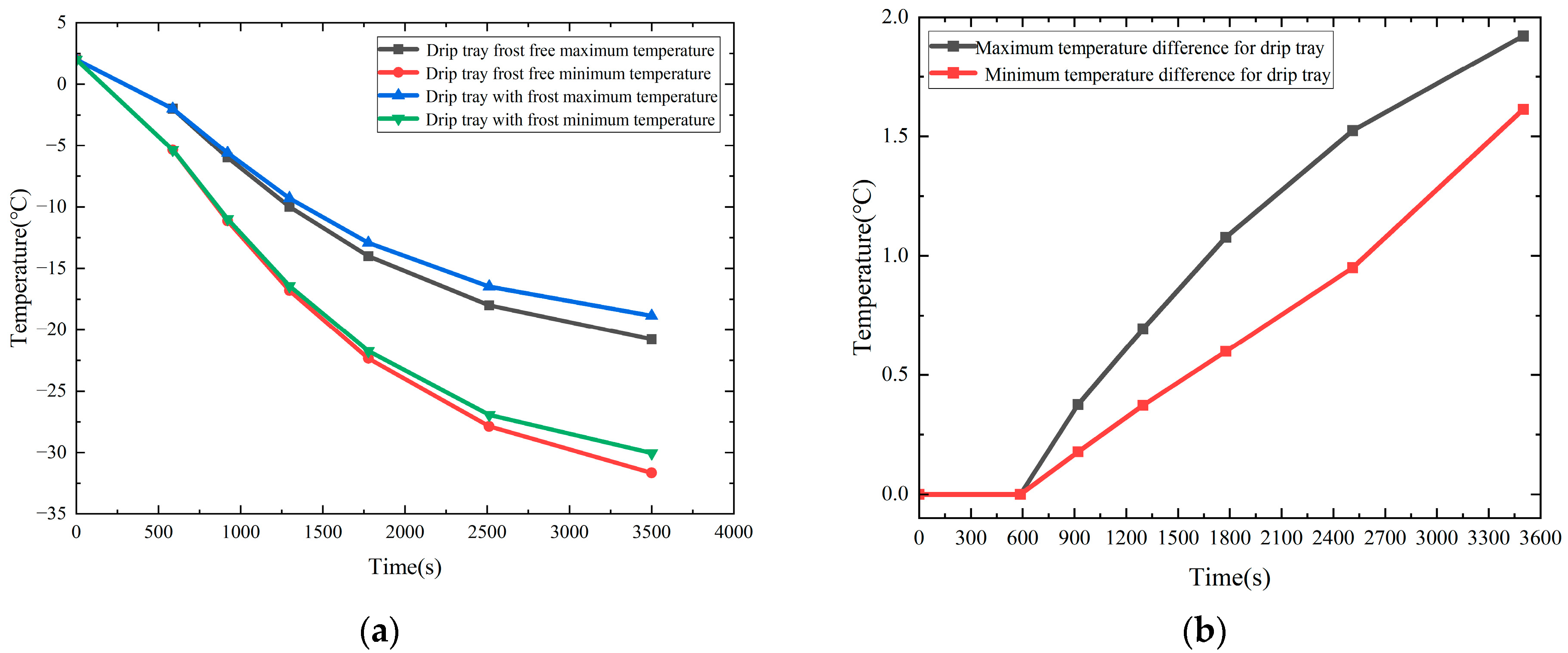In addition, Figure 18a compares the temperature variation in the drip tray with and without the presence of a frost layer, while Figure 18b demonstrates the trend in the temperature difference over time, caused by the presence of a frost layer.

When the drip tray is placed horizontally, condensate easily accumulates on its surface. As the condensate accumulates and the temperature of the drip-tray surface decreases, the accumulated water droplets begin to condense to form a frost layer and gradually thicken on the surface of the drip tray of the low-temperature ball valves, and so the frost layer has a very significant effect on the heat transfer characteristics of the drip tray. The drip-tray temperature conduction increases in temperature from the root to the external radial edge. That is, the drip-tray root temperature is the lowest, and the highest temperature is seen at the external edge of the drip tray. The heat transfer between the air and the drip tray decreases as the radius increases. The larger the radius of the drip tray, the smaller the difference between the surface temperature and the ambient temperature will be, and so an isothermal surface is formed as shown in the figure above. In terms of the influence of the frost layer on the heat transfer characteristics of the drip tray, it can be seen from Figure 18a,b, that, after 587 s, i.e., when the frost layer begins to appear on the surface of the drip tray, the influence of the frost layer on the maximum and minimum temperatures of the drip tray begins to appear. When the heat transfer time is 921 s, the height of the frost layer is 0.21 mm. At this time, due to the existence of the frost layer, the maximum and minimum temperatures of the drip tray are increased by 0.381 °C and 0.178 °C, respectively. Thereafter, with the conduction of the cold temperature at the bottom and the continuous growth of the frost layer, the temperature differences between the drip tray with and without the frost layer become larger and larger, showing a stable growth trend, and at 3500 s, the maximum and minimum temperature difference between the drip tray with and without the frost layer reach the maximum values seen during the observation process, which are 1.92 °C and 1.61 °C, respectively. It is worth noting that the curve of the maximum temperature difference in the drip trays showed an overall increasing trend with the advancement of time, but that the growth rate gradually slowed down. This phenomenon can be attributed to the growth of the frost layer. The formation of the frost layer not only expands the heat exchange area between the drip tray and the surrounding air, but also, due to its non-uniform distribution and surface roughness, makes the frost layer play a role similar to that of the finned radiators in enhancing heat exchange, which effectively improves the heat exchange efficiency of the surface of the low-temperature valves. This leads to an increase in the maximum temperature of the drip tray. However, with the continuous growth of the frost layer, the heat exchange thermal resistance of the surface of the drip tray also gradually increases, resulting in a reduction in the convective heat exchange between the surface of the drip tray and the air, thus reducing the heat dissipation efficiency of the drip tray and thus slowing down the trend of growth in the maximum temperature difference.

4.4.3. Comparative Analysis of Temperature Field With and Without Frost-Layer Stuffing Box

The key to a stuffing box is its sealing, and low temperatures can damage its sealing. Once the stuffing box is damaged and the LNG leaks, it will expand rapidly when it encounters air and may explode, and so it is vital to explore the effect of frost on the temperature of the stuffing box. The frosting of the drip tray affects its heat dissipation effect, which in turn affects the temperature of the stuffing box. In this study, the temperature field distribution of the stuffing box in the presence and absence of a frost layer was calculated by numerical simulation, as shown in Figure 19 and Figure 20. In addition, Figure 21a compares the variation in the stuffing-box temperature with and without the presence of a frost layer, while Figure 21b shows the trend in the temperature difference with time due to the presence of a frost layer.

Through the visual analysis of the heat transfer process, it can be observed that the distribution law of the stuffing-box temperature field is similar to that of the overall valve, showing a gradient of temperature distribution with a gradual increase in temperature from the bottom to the top. The formation of this temperature gradient is related to the upward conduction of the cold temperature at the bottom, and the overall temperature changes dynamically with the conduction of the cold temperature at the bottom and the growth of the frost layer. In terms of the influence of the frost layer on the heat transfer characteristics of the stuffing box, the influence of the frost layer on the temperature of the stuffing box is more intuitive compared to the influence of the overall maximum temperature of the valve because the drip tray is closer to the stuffing box. As can be seen from Figure 21a,b, the effect of the frost layer on the maximum and minimum temperatures of the stuffing box starts to appear after 587 s, when the frost layer starts to form on the surface of the drip tray. When the heat transfer time is 921 s and the height of the frost layer is 0.21 mm, the presence of the frost layer causes the maximum and minimum temperatures of the stuffing box to increase by 0.0637 °C and 0.0153 °C, respectively. With the conduction of cold temperature at the bottom and the continuous growth of the frost layer, the difference between the maximum and minimum temperatures of the stuffing box with and without the frost layer shows a steady upward trend. At 3500 s, this temperature difference reaches the maximum values observed, which are 0.445 °C and 0.752 °C, respectively. Obviously, when the frost layer affects the heat dissipation efficiency of the drip tray, it also directly affects the temperature of the valve stuffing box, and its influence on the heat transfer characteristics of the stuffing box becomes more and more significant as the frost layer continues to grow. This trend clearly shows that frost growth is a constant and critical factor in the heat transfer characteristics of the stuffing box.

5. Conclusions

This paper addresses the phenomenon where frost appears on the cold surface of low-temperature valves. The Eulerian multiphase flow model seen in Fluent software is used to numerically calculate the ice-phase volume fraction and the average height of the frost layer on the cold surface at different stages. The frost layer formed is coupled with the valve model, and the transient temperature field of the low-temperature valve coupled with a frost layer is numerically simulated using ANSYS Workbench finite element software. By combining theoretical analysis and numerical calculations, the effect of frost-layer growth on the heat transfer characteristics of cryogenic valves is investigated thoroughly. The results show the following outcomes:

(1)

During the simulation period of 3500 s, the formation of the frost layer increases the heat exchange area between the drip tray and the air, and due to its inhomogeneity and surface roughness, it plays a role similar to that of a finned radiator, thus improving the heat exchange efficiency on the surface of the drip tray. This leads to an increase in the temperature of the drip tray and the stuffing box in comparison with that of the no-frost-layer state.

(2)

Due to the existence of the frost layer, the heat emitted from the drip tray needs to be conducted to the surface of the frost layer first, and then transmitted by the frost layer and the surrounding air for convection heat transfer. With the growth of the frost layer, the thickness of the frost layer continues to increase. The increase in the thickness of the frost layer brings the surface of the drip tray into contact with the surface of the frost layer, extending the path of heat conduction. This, in turn, increases the thermal resistance to heat transfer, thereby reducing the cooling efficiency of the drip tray.

The findings of this study not only verify the dual role played by the frost layer in the heat transfer process of cryogenic valves, but also provide technical routes and important references for future cryogenic valves in the design and optimization of anti-deicing. We believe that these research results will help to promote the development of anti-icing and defrosting technologies for cryogenic valve components of polar LNG ships, which will support the safe operation and energy efficiency of polar LNG ships.