Article

Research on Water Flow Control Strategy for PEM Electrolyzer Considering the Anode Bubble Effect

College of Electrical Engineering, Xinjiang University, Urumqi 830017, China
*
Author to whom correspondence should be addressed.
Energies 2025, 18(2), 273; https://doi.org/10.3390/en18020273
Submission received: 18 December 2024 / Revised: 2 January 2025 / Accepted: 8 January 2025 / Published: 9 January 2025
(This article belongs to the Section A5: Hydrogen Energy)

Abstract

:
At higher current densities, the bubble effect in the anode flow field of the PEM electrolyzer (PEM EL) worsens mass transfer losses and energy consumption. This study employs a moderate increase in the water flow rate to remove accumulated bubbles under fluctuating electrical input, thereby improving PEM EL system efficiency. An enhanced PEM EL equivalent circuit model incorporating bubble over-potential based on the oxygen volume fraction is developed. Considering the energy consumption of auxiliary equipment and the reduction in losses from mitigating the bubble effect, a numerical simulation evaluates the impact of flow rate variations on overall electrolysis energy consumption, leading to a comprehensive energy consumption model for the PEM EL system, incorporating electrical, chemical, and thermal energy conversions. The control objective is to maximize system efficiency by optimizing the water flow rate, with a performance-preset-based controller implemented in MATLAB/Simulink. The simulation results show that the controller can accurately track the target flow rate, and the dynamic regulation time improved by 1.5 s compared to the traditional performance constraint function, better matching the rate of change in electrical energy. Under the water flow control mode, hydrogen production increased by 6.6 L within 130 s of the simulation, available energy increased by 8.32 × 10⁶ J, and the efficiency of the PEM EL system improved by 2.79%.

1. Introduction

Hydrogen, recognized as the clean energy carrier with the highest energy density, is considered the optimal alternative to fossil fuels [1]. Among various water electrolysis technologies, the PEM electrolyzer (PEM EL) has garnered considerable attention due to its advantages, including a wide operating power range, high current density, high hydrogen production efficiency, high hydrogen purity, and rapid dynamic response time [2]. A typical PEM EL system, in addition to the electrolyzer, consists of auxiliary components such as an adjustable DC power source, water pump, hydrogen storage tank, and heater. These auxiliary devices regulate key variables, including current, voltage, temperature, pressure, power, and water flow rate, all of which directly influence the performance of the electrolyzer.
Reference [3] found that ripples and fluctuations in input current and voltage increase ion vibrations and generate Joule heating, leading to a reduction in hydrogen production efficiency. Research in [4,5,6] indicates that, within the safe operating temperature range, an increase in temperature can effectively lower over-potential and enhance the hydrogen production efficiency, while excessively high temperatures may damage the proton exchange membrane. References [7,8] found that performing electrolysis under high-pressure conditions (close to hydrogen storage pressure) eliminates the need for a compressor, thereby reducing energy consumption and improving hydrogen production efficiency. Reference [9] discovered that during a four-month period of direct coupling between a photovoltaic source and a PEM EL, the efficiency dropped from 91% to 65% due to power fluctuations and intermittency, which degraded the electrolyzer’s performance. Reference [10] proposes a power management system for off-grid renewable energy (PV and wind) hydrogen production, integrating fuzzy logic control and power prediction to minimize electrolyzer startup and shutdown frequency, thus mitigating the degradation of electrolysis performance.
However, as water is a crucial reactant in the PEM EL, most studies have not thoroughly investigated the effect of water supply flow on hydrogen production performance. References [11,12] derived the relationship between water consumption in the electrolysis reaction and photovoltaic output power, with the goal of matching the water flow rate to photovoltaic power in order to maximize energy utilization efficiency. However, they did not account for the fact that low water flow rates could lead to excessive temperatures and accelerate the aging of the electrolyzer. Reference [13] employed the water supply system as a cooling mechanism and concluded that a water flow rate slightly exceeding consumption can prevent the proton exchange membrane from drying out and help maintain a reasonable temperature. However, in the absence of a recirculation system, this approach increased water pump energy consumption and heat waste, while overlooking the direct impact of water flow on bubble coverage. Therefore, this study adopts a separate water supply for the anode to fully utilize the Joule heat generated by electrolysis and proposes to increase the water supply flow rate to thousands of times higher than the theoretical flow rate required, considering the bubble effect. This approach not only enhances electrolysis efficiency but also effectively maintains the temperature within a reasonable range and prevents the drying out of the proton exchange membrane due to elevated temperatures.
Since the bubble effect significantly impacts anode over-potential [14], this study focuses on the control strategy for anode circulation water flow in the PEM EL system to enhance electrolysis efficiency. First, an equivalent circuit model of the PEM EL, which incorporates bubble over-potential, is established using the oxygen volume fraction. This model analyzes the impact of input electrical energy on system performance and constructs an energy consumption model for the PEM EL system. Next, under constant current density conditions, numerical simulations are conducted to analyze the impact of flow rate changes on electrolysis energy consumption. The analysis also considers the energy consumption of auxiliary equipment, such as water pumps, and the energy savings resulting from mitigating bubble effects, with the flow rate that maximizes overall system efficiency serving as the control target. Finally, a water flow controller based on the performance preset method is designed in MATLAB/Simulink R2021b, and its effectiveness is validated by comparing it with an uncontrolled mode under fluctuating power conditions.

2. Modeling of PEM EL

A PEM EL model was developed in COMSOL 6.2, integrating two-phase flow (k-ε module and free and porous media flow module), electrochemistry (water electrolyzer module), and heat transfer (heat transfer in fluids and solids module). Detailed equations and theoretical foundations are provided in the relevant modules of the COMSOL Multiphysics documentation. The physical parameters of the model are detailed in Appendix A.
Particularly, this study models the bubble effect as an equivalent resistance on the anode side, with the oxygen volume fraction used to adjust the operating current in the ohmic over-potential.

2.1. Electrolyzer Multi-Physics Field Model

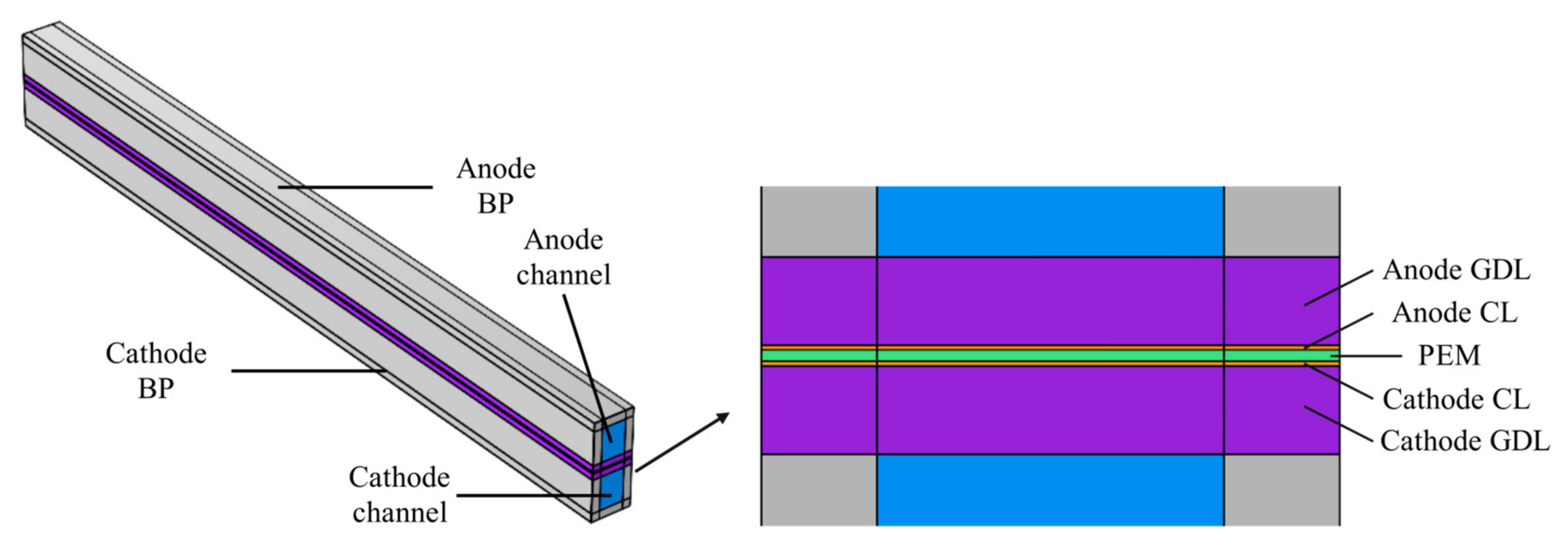
2.1.1. Geometric Model

Figure 1 presents a typical single-channel model of the PEM EL, representing the fundamental unit of the flow field. The physical domain includes the bipolar plate, flow channel, gas diffusion layer (GDL), catalyst layer (CL), and PEM (Nafion112, 50 μm). On the anode side, the flow channel is supplied with a pure water inlet and an outlet for the gas–liquid mixture. In contrast, the cathode side does not have a direct water supply; however, water can permeate from the anode to the cathode through the proton exchange membrane during the electrolysis process. As a result, the cathode channel includes only an outlet for the gas–liquid mixture. The anode and cathode channels are symmetric.

2.1.2. Model Assumption

To simplify the model while maintaining computational accuracy, the following reasonable assumptions are made:
  • The PEM, GDLs, and CLs are isotropic and homogeneous.
  • The water evaporation is ignored, as the reactants mainly exist in liquid form under operating conditions.
  • All gasses are treated as incompressible ideal gasses.
  • Hydrogen and oxygen crossovers are disregarded.
  • The contact resistance between adjacent components is not considered.

2.1.3. Boundary Condition Setting and Model Verification

In this study, a constant potential boundary condition is applied. The anode plate end face is set to a fixed potential, while the cathode plate end face is set to 0 V. The remaining external walls are electrically insulated. The anode inlet is specified as a velocity inlet, with the anode and cathode outlets set as pressure outlets. No-slip boundary conditions are applied to all other fluid region walls. The top and bottom walls of the cell are maintained at a constant temperature, while the remaining side and end walls are treated as adiabatic.
The grid cell size was gradually refined and the current density was calculated at 0.05 m/s, 2 V. The grid independence is shown in Table 1. It can be seen that the errors of the current density are all within 4% and gradually decreasing, and their errors are within a reasonable range. In order to balance the accuracy and efficiency of the calculation, the number of grids is selected as 44,795 for subsequent calculations.
Validation of the proposed model: under the same geometrical conditions and working conditions, the simulation data are compared with the experimental data from the literature [15]. The results are shown in Figure 2; the simulations are good, and the errors are all within 10%.

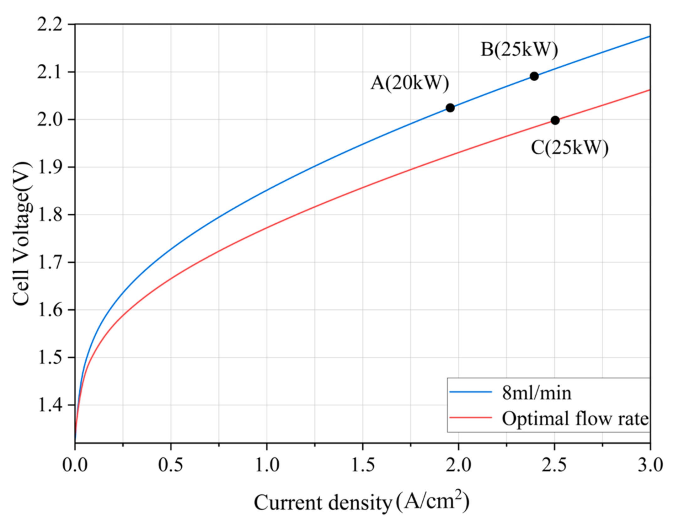
2.2. Impact of Water Flow Rate Variation on Electrolysis Energy Consumption

An increase in the water flow rate results in several effects within the PEM EL: increased heat loss, lowering the operating temperature; enhanced expulsion of oxygen bubbles, reducing mass transfer losses; higher energy consumption due to the additional power required by the pump.
Under a 2 V voltage input, the dynamic process of increasing the water pump flow rate from 3 to 20 mL·min−1 over 2 s was simulated. As shown in Figure 3a, the oxygen volume fraction in the anode CL decreases gradually with increasing flow rate, stabilizing after approximately 1.5 s. Figure 3b illustrates that the volumetric current density in the CL increases with higher water flow rates (and reduced oxygen fraction) as the enhanced flow facilitates the expulsion of oxygen bubbles, thereby reducing mass transfer losses.
Figure 4 shows that variations in water flow rate have a minimal effect on the temperature distribution within the CL under a 2 V input. While the temperature slightly decreases with higher flow rates, the maximum temperature difference remains within 3 K. This phenomenon can be explained as follows: although an increase in the water flow rate removes more heat from the electrolyzer, the corresponding increase in current density generates additional Joule heat, which counteracts the heat loss, leading to only a minor change in temperature. Consequently, the influence of flow rate on temperature is not a significant factor in the observed differences in electrolysis performance.
The proton exchange membrane remains the weakest part of the PEM cell [16]. Long-term uneven temperature distribution may lead to thinning in the proton exchange membrane and consequent damage, but a small degree of uneven temperature distribution is unavoidable. The current thermal management strategy for PEM electrolysis tanks involves regulating the water supply’s temperature and flow rate to promote a more uniform temperature profile. The flow control strategy proposed in this study can achieve comparable results. The current water supply temperature of 338.15 K is a safe and reliable value, even with a small temperature rise; it remains within a reasonable range, and furthermore, concerns regarding the effects of temperature changes during flow control are unwarranted.

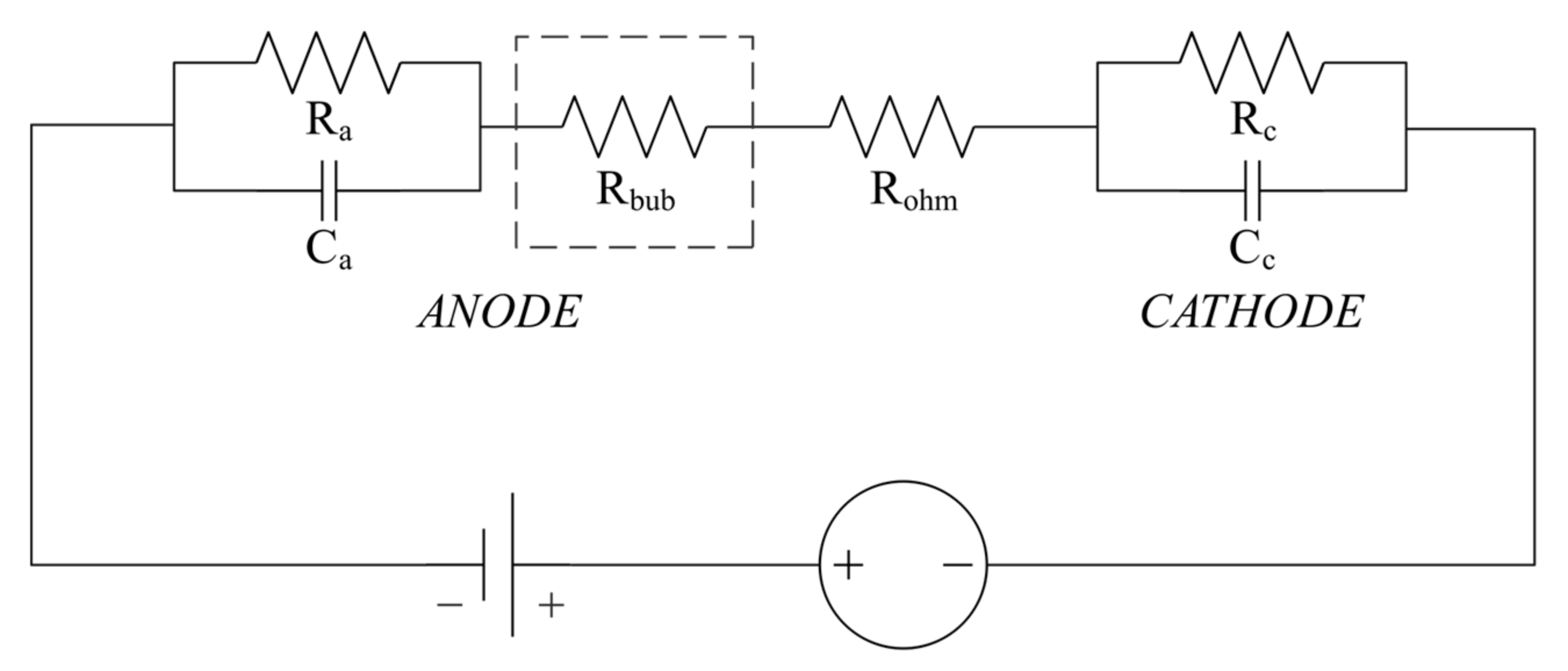
2.3. Revised Electrolyzer Equivalent Circuit Model

In order to facilitate the simulation of the subsequent controller simulation, the second-order RC equivalent circuit of the modified PEM EL, including the bubble effect, is constructed.
Typically, the voltage of the electrolyzer is expressed as the sum of its reversible potential and over-potential:
V cell = E eq + V act + V ohm + V con
where E eq is the reversible potential, V act is the activation over-potential, V ohm is the ohmic over-potential, and V con is the concentration over-potential. The specific expressions for over-potential and the heat/mass transfer models are provided in references [17,18,19,20,21,22,23,24].
The corrected operating current I eff is as follows:
I eff = I cell / ( 1 θ mem )
where θ mem is the average oxygen volume fraction at the membrane—electrode interface, and the over-potential caused by oxygen bubbles is as follows:
V bub = R bub I cell = R ohm I cell θ mem / ( 1 θ mem )
The average oxygen volume fraction is given by the following [25]:
θ mem = V ˙ O 2 V ˙ O 2 + V ˙ H 2 O = I cell 10 6 R T 4 F P an I cell 10 6 R T 4 F P an + M H 2 O ρ H 2 O ( I cell 2 F + 4 I cell F ) = 10 6 R T 4 P an 10 6 R T 4 P an + ( 0.5 + 4 ) M H 2 O ρ H 2 O
where V ˙ O 2 is the oxygen volumetric flow rate, V ˙ H 2 O is the water volumetric flow rate, P an is the anode pressure, ρ H 2 O (g·cm−3) is the density of water, M H 2 O (g·mol−1) is the molar mass of water, T is the temperature, R is the ideal gas constant, and F is the Faraday constant.
The revised equivalent circuit is presented in Figure 5.
The equivalent resistances R a and R c and the equivalent capacitances C a and C c are estimated as functions of the operating current, as given in reference [26].

3. Design of the Water Flow Rate Controller

3.1. Determining the Control Objective

Figure 6 shows the schematic of the PEM EL system structure. In addition to the electrolyzer, the system comprises components such as adjustable DC/DC power supplies, a water tank, a water pump, a gas–water separator, a hydrogen compressor, a hydrogen storage tank, and a heat exchanger.
The electrical energy supplied to the PEM EL system is converted into both chemical and thermal energy. A portion of the thermal energy, along with all of the chemical energy, is utilized in the electrolysis reaction. The excess thermal energy increases the water temperature, which is then circulated through the system, with only a small fraction dissipating through the pipes or being expelled along with the gas bubbles. The increase in electrical energy results in greater gas production, further raising the ohmic overvoltage, including the bubble overvoltage. The total energy consumption of the PEM EL system is the sum of the electrical energy consumed by the PEM EL, the circulating water pump, and the hydrogen compressor:
W cell = 0 t U cell I cell d t W pump = 0 t Q A d t H ρ H 2 O / 0.75 W cp = 0 t Q H 2 d t Δ P ρ H 2 / 0.8
where W cell is the energy consumed by PEM EL, U cell is the voltage of the PEM EL, W pump is the energy consumed by the water pump, Q A is the actual flow rate of the pump, H is the pump head, 0.75 is the pump’s efficiency, W cp is the energy consumed by the hydrogen compressor, Q H 2 is the hydrogen flow rate, Δ P is the pressure difference between the compressor inlet and outlet, ρ H 2 is the density of hydrogen, and 0.8 is the hydrogen compressor’s efficiency.
Based on the preceding analysis, increasing the flow rate under fixed electrolysis power can enhance performance. The optimal water supply flow rate is determined by maximizing the balance between reduced mass transfer losses and the energy consumption of the water pump. Electrolysis efficiency is as follows:
η cell = W H 2 / ( W cell + W pump + W cp )
where W H 2 is the higher heating value (HHV) of the hydrogen.
Obviously, after taking into account the energy consumption of the pump, there exists an optimal working condition of the electrolysis system, when the electrolysis efficiency is maximum. By setting different flow rates and solving the polarization curve in COMSOL, the optimal water supply flow rate curve can be obtained based on (5) and (6), and the optimal flow rate can be identified using an offline lookup table.
As shown in Figure 7, when the input power of the PEM EL system changes, its operating point moves from point A to point B through voltage regulation by an adjustable DC source, ensuring that the electrolyzer power P equals the power command P(k). Then, the optimal water supply flow rate Qop(k) for that power level is determined, and the water pump is adjusted so that the operating point ultimately reaches point C, where the PEM EL system achieves maximum efficiency under the new power input.
The control process is illustrated in Figure 8. This study does not involve the control of hydrogen production power sources, only the control of water supply flow rate.

3.2. Water Flow Rate Controller

3.2.1. Circulating Water Pump Model

It is known that the water pump flow rate is proportional to its rotational speed, and the flow rate equation can be expressed as follows: Q ( t ) = k N ( t ) , where N ( t ) (r·min−1) is the rotational speed of the water pump, and k (L·r−1) is the displacement of the pump. The dynamics of the system can be represented as a first-order system:
N ˙ ( t ) = ( u N ( t ) ) / T c
where u is the input rotational speed command, and T c is the response time constant of the water pump. Thus, the differential equation for the flow rate can be obtained:
Q ˙ ( t ) = ( Q ( t ) + k u ) / T c

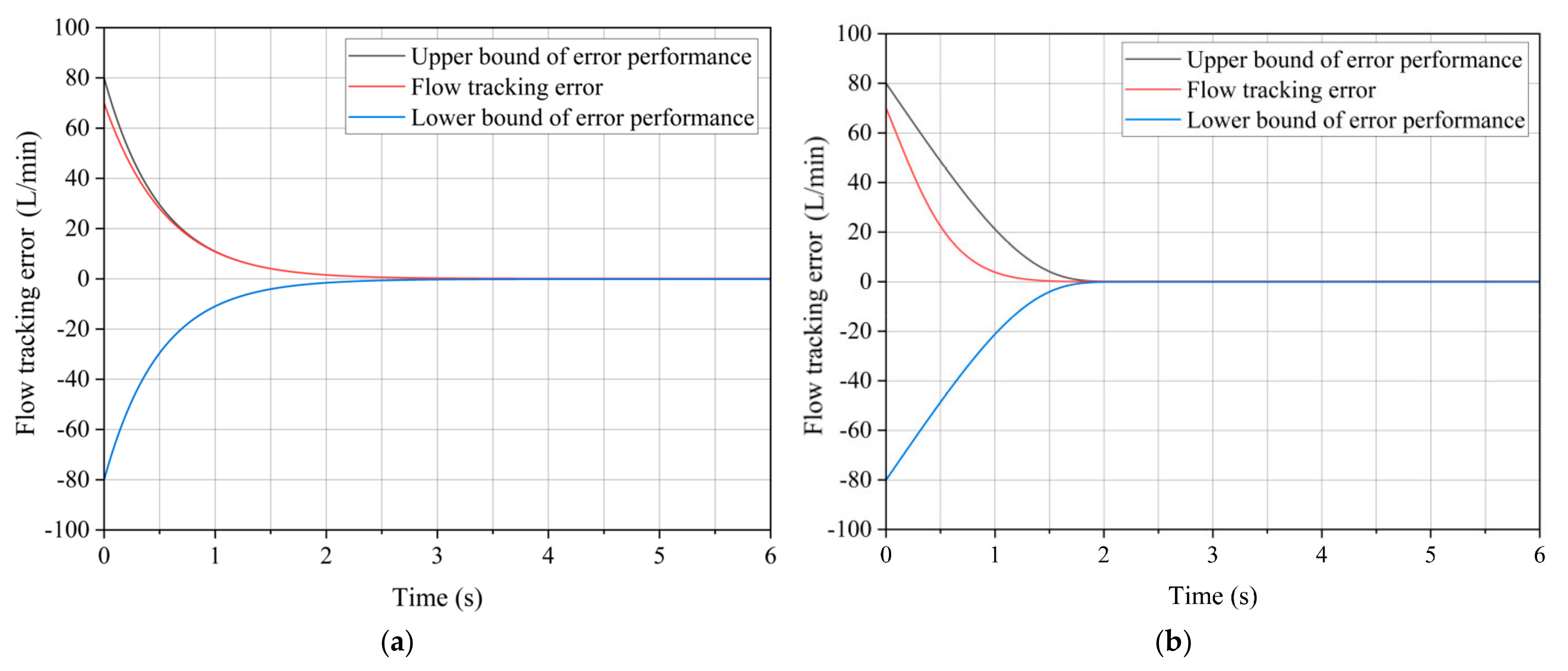
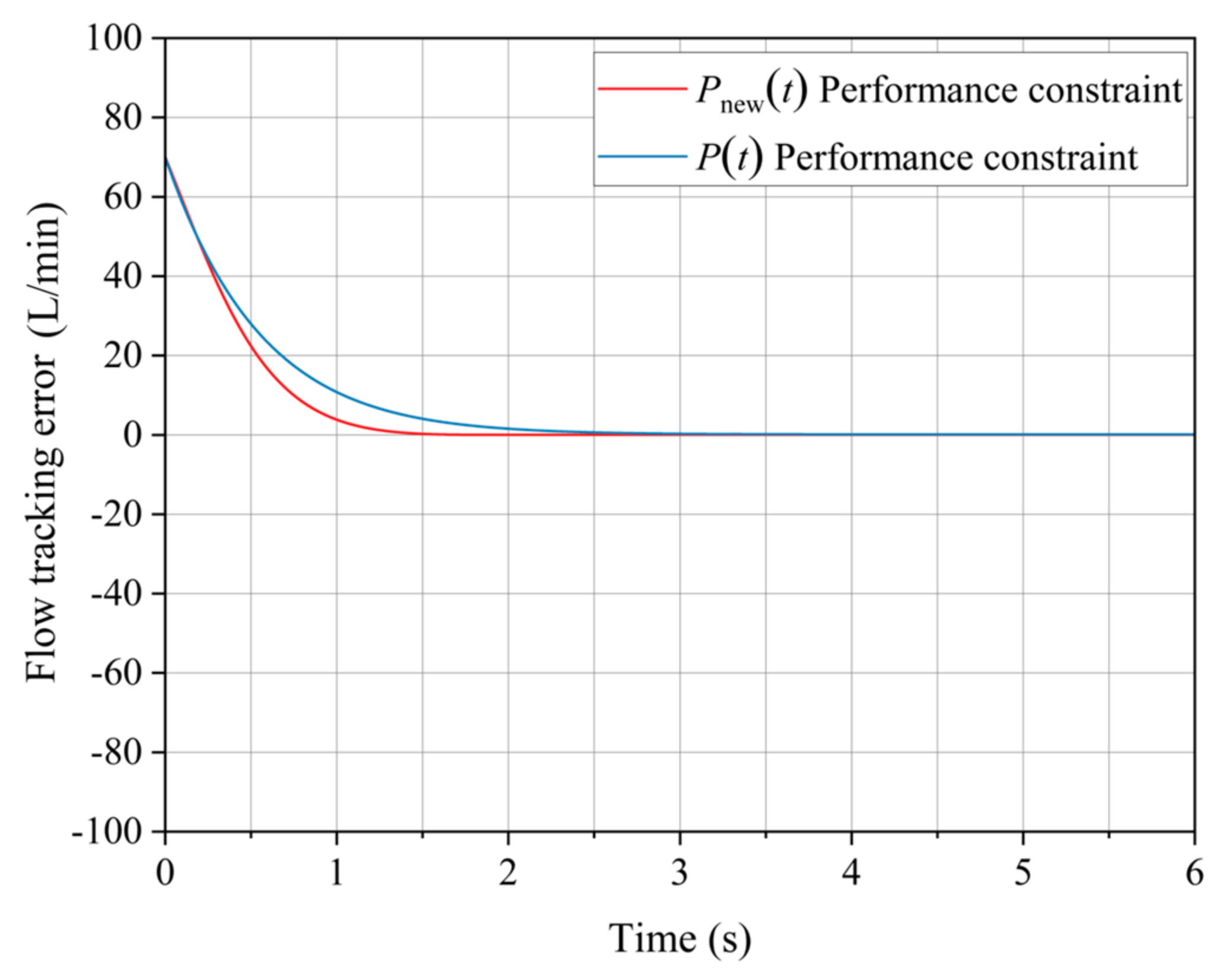
3.2.2. Performance Preset Control

Define the flow-tracking error: e ( t ) = Q d ( t ) Q ( t ) , where Q d ( t ) is the desired water flow rate. Differentiating e ( t ) yields the following:
e ˙ ( t ) = Q ˙ d ( t ) + ( Q ( t ) k u ) / T c
Next, the performance preset method is employed for the controller design, and the performance function, which is positive and monotonically decreasing within the defined time domain, is defined as follows:
P ( t ) = ( P ( 0 ) P ( ) ) exp ( β t ) + P ( )
where P ( 0 ) and P ( ) are the initial and steady-state values of P ( t ) , β determines the lower bound of the tracking-error convergence rate, and exp β t is the decay factor.
To accelerate error convergence, forms of improvement to the performance function are made and compared:
P new ( t ) = ( P ( 0 ) P ( ) ) exp ( β t T t ) + P ( ) ,   t < T P ( ) ,   t T
where when tT, the function decays to 0. Obviously, the regulation time of the pump flow can be preset by this performance function to reach its own fastest regulation speed to match the rapid change in electrical energy.

3.2.3. Calculation of Control Rate

Construct the error boundary:
δ P ( t ) < e ( t ) < P ( t )
where δ = −1.
To avoid increased complexity in controller design due to performance constraints, an equivalent mapping function (which should be smooth, invertible, and strictly increasing) is introduced to map the constrained space homeomorphically to an unconstrained space. Hence, the following error transformation is introduced:
e ( t ) = P i ( t ) T ( ε , δ )
where:
T ( ε , δ ) = exp ε exp ( ε ) exp ε + δ 1 exp ( ε )
where ε is the transformed error. The transformation function T ( ε , δ ) must satisfy the following:
δ < T ( ε , δ ) < 1 ,   ε L lim ε T ( ε , δ ) = δ lim ε T ( ε , δ ) = 1
where L denotes boundedness. Solving for ε results in the following:
ε = T ( e * ) = 1 2 ln ( δ + e * δ δ e * )
where e * = e ( t ) / P i ( t ) is the normalized error. T ( ε , δ ) transforms the error from its constrained space to the real number space, with the transformed error ε ( , + ) , indicating the system is unconstrained. The performance constraint of the error will be satisfied if and only if the transformed error is bounded. Differentiate ε :
ε ˙ = p e ˙ ( t ) q e ( t )
where:
p = 1 2 P ( t ) [ 1 δ + T ( ε , δ ) + 1 1 T ( ε , δ ) ] q = 1 2 [ δ P ˙ ( t ) δ P ( t ) ( δ P ( t ) + e ( t ) ) + P ˙ ( t ) P ( t ) ( P ( t ) e ( t ) ) ]
Combining with (9), the new system state equation can be obtained:
ε ˙ new = p ( Q ˙ d ( t ) + Q ( t ) k u T c ) q e ( t )
Using the second method of Lyapunov to solve for the system control rate: Let V = 1 2 ε 2 , then: V ˙ = ε ε ˙ ; let ε = k 1 ε (k1 > 0, is the gain). Clearly, at this point, V ˙ < 0 . Consequently, the control rate can be obtained:
u = T c k p ( q e ( t ) k 1 ε ) + T c Q ˙ d ( t ) + Q ( t ) k

4. Results

The PEM EL system is constructed using a linear stacking method, assuming that the water flow is evenly distributed to each cell. The detailed operating parameters of the electrolysis system are presented in Table 2.

4.1. Comparison of Water Flow Rate Tracking Performance

For the comparability of simulation results, T = 2.5 s in performance function P new ( t ) . The remaining parameters in the performance function are set as follows: P ( 0 ) = 80, P ( ) = 0.1, β = 2, δ = 1, and k1 = 2.
Figure 9 shows that both methods effectively track the flow changes, with no noticeable overshoot in either case. However, under the traditional constraint of the performance function P(t), the flow rate error decays very slowly and only decays to within the error allowance at about 3 s. Under the improved performance function Pnew(t) constraint, the error has reached the allowable margin of error at about 1.5 s.
As shown in Figure 10, under the constraints of performance improvement functionality, the water pump’s flow rate regulation performance is superior, with a reduction in dynamic adjustment time by 1.5 s. This indicates that the system’s responsiveness has been enhanced, which is a critical factor in the efficiency of flow rate regulation.

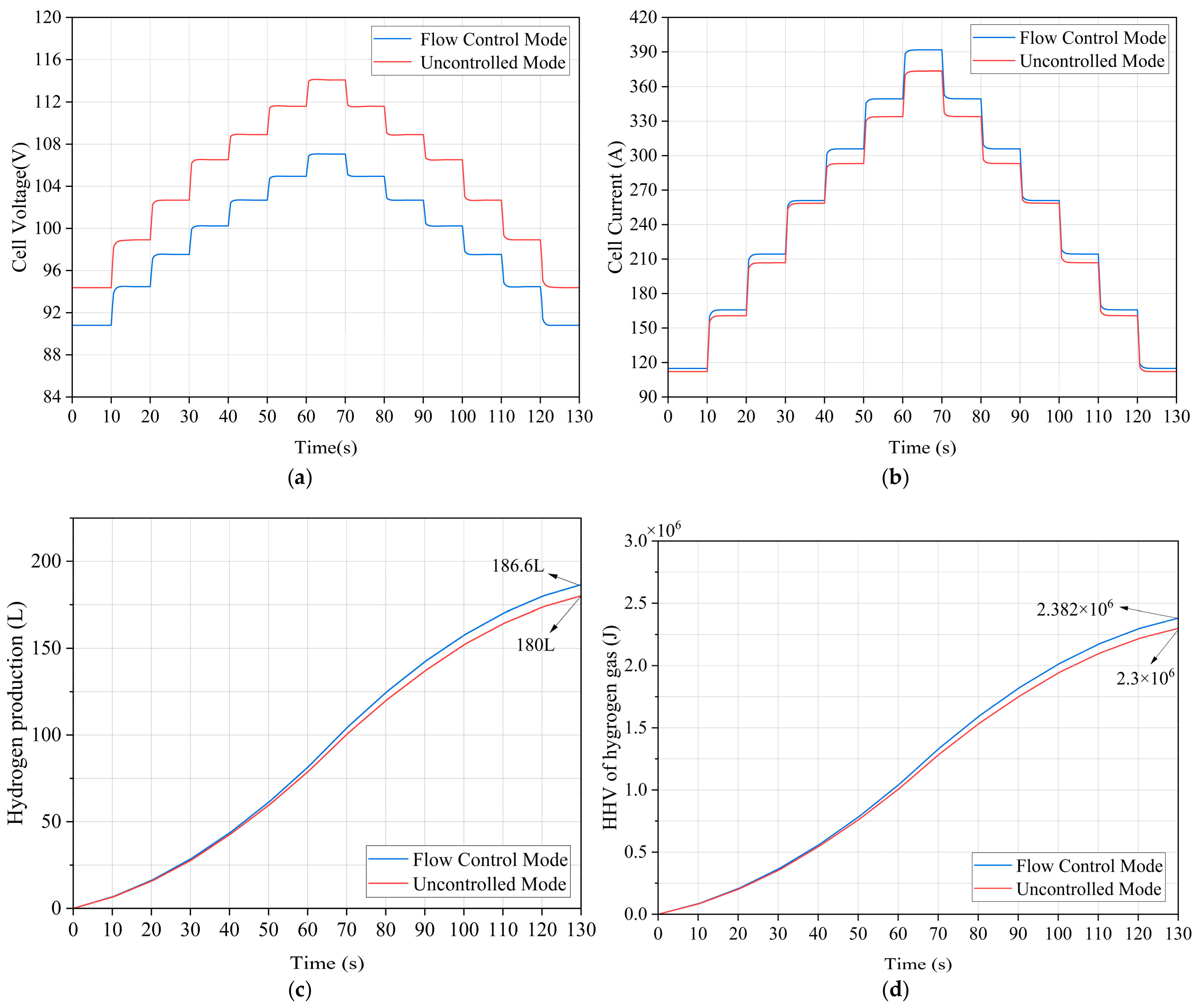
4.2. Impact of Water Flow Control on PEM EL Performance with Variable Power Input

A simple simulation of power system dispatch commands during fluctuations in renewable energy output is performed to compare the performance of the electrolysis system under variable power input. The power variations are shown in Figure 11.
From Figure 12a, it can be seen that the electrolyzer voltage is significantly reduced in water flow control mode, and the effect is more significant with higher input power. The overvoltage loss in the electrolyzer is reduced by about 7 V at 44 kW input power. From Figure 12b, it is seen that the electrolyzer current is significantly higher in the water flow control mode, by about 18.2 A at 44 kW input power. This implies lower energy consumption and greater hydrogen production. Figure 12c indicates that at 130 s, the hydrogen production in the flow-controlled mode is 186.6 L, which is 6.6 L greater compared to the uncontrolled mode; as can be seen from Figure 12d, this corresponds to an increase of 8.32 × 10⁴ J in available energy.
During the 130 s of simulation, as illustrated in Figure 13a, the system efficiency in flow control mode improved by 2.79% compared to the uncontrolled mode. As illustrated in Figure 13b, the total energy consumption is 3.41 × 10⁶ J, with the energy consumption of the PEM EL at 3.245 × 10⁶ J, representing 95.14% of the total energy consumption. The energy consumption of the hydrogen compressor is 1.173 × 10⁵ J, representing 3.44% of the total energy consumption, and the energy consumption of the water pump is 4.837 × 10⁴ J, accounting for 1.42% of the total energy consumption. The energy consumption attributed to the water pump is minimal, indicating that as the input power to the electrolyzer increases, its proportion will continue to decrease, thereby enhancing overall efficiency.

5. Discussion

This study analyzes the influence of water supply flow rate on the bubble effect by establishing a multi-physics field model of PEM EL in three dimensions, and propose a water flow rate control strategy for PEM EL based on the performance preset control, which improves the efficiency of the electrolysis system by increasing the water flow rate. The stability of the flow control system is analyzed and ensured by Lyapunov stability. To verify the effectiveness of the control strategy, different comparative simulation experiments are carried out and the results show that:
  • The improved performance function significantly improves the dynamic response time of the water flow rate error tracking, so that the pump flow regulation better matches the electrical energy input variation.
  • Under the flow control mode, the operating current of the electrolyzer rises, the overvoltage decreases significantly, and the electrolysis efficiency improves by 2.6% on average within 130 s of the simulation, proving the superiority of the proposed strategy.
  • The proposed water flow control strategy provides a method to find the optimal working point of the electrolysis system. It can determine the respective optimal water supply flow rate for different models of electrolyzers in engineering practice, avoiding the waste of energy and loss of efficiency.
Theoretically, the prompt removal of all oxygen generated during the reaction could enhance hydrogen production efficiency by more than 20%. However, adjusting the water supply flow rate achieves only a 2–3% improvement in electrolysis efficiency, falling far short of the ideal outcome. Future research could explore optimizing operating pressure, materials, and flow field structures of the PEM EL to improve oxygen expulsion and achieve more efficient operation.

Author Contributions

Conceptualization, Y.T. and L.A.; methodology, L.A. and H.Z.; software, L.A.; validation, L.A.; formal analysis, L.A. and H.Z.; investigation, Y.T. and L.A.; resources, Y.T.; data curation, L.A.; writing—original draft preparation, L.A.; writing—review and editing, L.A.; visualization, L.A.; supervision, Y.T.; project administration, Y.T.; funding acquisition, Y.T. All authors have read and agreed to the published version of the manuscript.

Funding

This study was supported in part by the Research on comprehensive utilization model of solar energy based on aggregation and frequency division (2022D01C364).

Data Availability Statement

The original contributions presented in the study are included in the article, further inquiries can be directed to the corresponding author.

Acknowledgments

We would like to express our appreciation to Y.T. for inspiring our collective interest in the development of innovative technologies. The guidance and insights provided by Y.T. have been invaluable to each member of our team, contributing significantly to our shared enthusiasm for this field.

Conflicts of Interest

The authors declare no conflicts of interest.

Appendix A

Table A1. Relevant Parameters of the Multiphysics Field Model.
ParameterValue
Channel length100 mm
Channel height2 mm
Channel width1.5 mm
Channel spacing1 mm
Thickness of CLs20 µm
Thickness of GDLs380 µm
PEM thickness50 µm
Anode reversible potential1.229 V
Cathode reversible potential0 V
Anode entropy change326.36 J·mol−1·K−1
Cathode entropy change−0.104 J·mol−1·K−1
Bipolar plate conductivity5 × 107 S·m−1
Conductivity of GDLs1.2 × 104 S·m−1
Conductivity of CLs3 × 103 S·m−1
Cathode specific active surface area6 × 107 m−1
Anode specific active surface area6 × 107 m−1
Transfer coefficients of the cathode electrode0.5
Transfer coefficients of the anode electrode0.5
Cathode reference exchange current density2.5 × 107 A·cm−2
Anode reference exchange current density5 × 103 A·cm−2
Gas pore volume fraction0.4
Gas pore tortuosity1.5
Electrolyte volume fraction0.3

References

  1. Wang, M.; Wang, Z.; Gong, X.; Guo, Z. The intensification technologies to water electrolysis for hydrogen production—A review. Renew. Sustain. Energy Rev. 2014, 29, 573–588. [Google Scholar] [CrossRef]
  2. Carmo, M.; Fritz, D.L.; Mergel, J.; Stolten, D. A comprehensive review on PEM water electrolysis. Int. J. Hydrogen Energy 2013, 38, 4901–4934. [Google Scholar] [CrossRef]
  3. Guilbert, D.; Vitale, G. Improved Hydrogen-Production-Based Power Management Control of a Wind Turbine Conversion System Coupled with Multistack Proton Exchange Membrane Electrolyzers. Energies 2020, 13, 1239. [Google Scholar] [CrossRef]
  4. Ali, D.; Gazey, R.; Aklil, D. Developing a thermally compensated electrolyser model coupled with pressurised hydrogen storage for modelling the energy efficiency of hydrogen energy storage systems and identifying their operation performance issues. Renew. Sustain. Energy Rev. 2016, 66, 27–37. [Google Scholar] [CrossRef]
  5. Petipas, F.; Brisse, A.; Bouallou, C. Benefits of external heat sources for high temperature electrolyser systems. Int. J. Hydrogen Energy 2014, 39, 5505–5513. [Google Scholar] [CrossRef]
  6. Polonský, J.; Mazúr, P.; Paidar, M.; Christensen, E.; Bouzek, K. Performance of a PEM water electrolyser using a TaC-supported iridium oxide electrocatalyst. Int. J. Hydrogen Energy 2014, 39, 3072–3078. [Google Scholar] [CrossRef]
  7. Onda, K.; Kyakuno, T.; Hattori, K.; Ito, K. Prediction of production power for high-pressure hydrogen by high-pressure water electrolysis. J. Power Sources 2004, 132, 64–70. [Google Scholar] [CrossRef]
  8. Degiorgis, L.; Santarelli, M.; Calì, M. Hydrogen from renewable energy: A pilot plant for thermal production and mobility. J. Power Sources 2007, 171, 237–246. [Google Scholar] [CrossRef]
  9. Clarke, R.E.; Giddey, S.; Ciacchi, F.T.; Badwal, S.P.S.; Paul, B.; Andrews, J. Direct coupling of an electrolyser to a solar PV system for generating hydrogen. Int. J. Hydrogen Energy 2009, 34, 2531–2542. [Google Scholar] [CrossRef]
  10. Cano, M.H.; Kelouwani, S.; Agbossou, K.; Dubé, Y. Power management system for off-grid hydrogen production based on uncertainty. Int. J. Hydrogen Energy 2015, 40, 7260–7272. [Google Scholar] [CrossRef]
  11. Dahbi, S.; Aboutni, R.; Aziz, A.; Benazzi, N.; Elhafyani, M.; Kassmi, K. Optimised hydrogen production by a photovoltaic-electrolysis system DC/DC converter and water flow controller. Int. J. Hydrogen Energy 2016, 41, 20858–20866. [Google Scholar] [CrossRef]
  12. Derbal-Mokrane, H.; Benzaoui, A.; M’Raoui, A.; Belhamel, M. Feasibility study for hydrogen production using hybrid solar power in Algeria. Int. J. Hydrogen Energy 2011, 36, 4198–4207. [Google Scholar] [CrossRef]
  13. Oi, T.; Sakaki, Y. Optimum hydrogen generation capacity and current density of the PEM-type water electrolyzer operated only during the off-peak period of electricity demand. J. Power Sources 2004, 129, 229–237. [Google Scholar] [CrossRef]
  14. Ojong, E.T.; Kwan, J.T.H.; Nouri-Khorasani, A.; Bonakdarpour, A.; Wilkinson, D.P.; Smolinka, T. Development of an experimentally validated semi-empirical fully-coupled performance model of a PEM electrolysis cell with a 3-D structured porous transport layer. Int. J. Hydrogen Energy 2017, 42, 25831–25847. [Google Scholar] [CrossRef]
  15. Baniasadi, S.T.A. Metal foams as flow distributors in comparison with serpentine and parallel flow fields in proton exchange membrane electrolyzer cells. Electrochim. Acta 2018, 290, 506–519. [Google Scholar]
  16. Millet, P.; Ranjbari, A.; de Guglielmo, F.; Grigoriev, S.A.; Auprêtre, F. Cell failure mechanisms in PEM water electrolyzers. Int. J. Hydrogen Energy 2012, 37, 17478–17487. [Google Scholar] [CrossRef]
  17. Afshari, E.; Khodabakhsh, S.; Jahantigh, N.; Toghyani, S. Performance assessment of gas crossover phenomenon and water transport mechanism in high pressure PEM electrolyzer. Int. J. Hydrogen Energy 2021, 46, 11029–11040. [Google Scholar] [CrossRef]
  18. Keller, R.; Rauls, E.; Hehemann, M.; Müller, M.; Carmo, M. An adaptive model-based feedforward temperature control of a 100 kW PEM electrolyzer. Control Eng. Pract. 2022, 120, 104992. [Google Scholar] [CrossRef]
  19. Zhao, D.; He, Q.; Yu, J.; Guo, M.; Fu, J.; Li, X.; Ni, M. A data-driven digital-twin model and control of high temperature proton exchange membrane electrolyzer cells. Int. J. Hydrogen Energy 2022, 47, 8687–8699. [Google Scholar] [CrossRef]
  20. Moradi Nafchi, F.; Afshari, E.; Baniasadi, E.; Javani, N. A parametric study of polymer membrane electrolyser performance, energy and exergy analyses. Int. J. Hydrogen Energy 2019, 44, 18662–18670. [Google Scholar] [CrossRef]
  21. Tijani, A.S.; Ghani, M.F.A.; Rahim, A.H.A.; Muritala, I.K.; Binti Mazlan, F.A. Electrochemical characteristics of (PEM) electrolyzer under influence of charge transfer coefficient. Int. J. Hydrogen Energy 2019, 44, 27177–27189. [Google Scholar] [CrossRef]
  22. Schnuelle, C.; Wassermann, T.; Fuhrlaender, D.; Zondervan, E. Dynamic hydrogen production from PV & wind direct electricity supply—Modeling and techno-economic assessment. Int. J. Hydrogen Energy 2020, 45, 29938–29952. [Google Scholar]
  23. Espinosa-López, M.; Darras, C.; Poggi, P.; Glises, R.; Baucour, P.; Rakotondrainibe, A.; Besse, S.; Serre-Combe, P. Modelling and experimental validation of a 46 kW PEM high pressure water electrolyzer. Renew. Energy 2018, 119, 160–173. [Google Scholar] [CrossRef]
  24. Abdin, Z.; Webb, C.J.; Gray, E.M. Modelling and simulation of a proton exchange membrane (PEM) electrolyser cell. Int. J. Hydrogen Energy 2015, 40, 13243–13257. [Google Scholar] [CrossRef]
  25. Villagra, A.; Millet, P. An analysis of PEM water electrolysis cells operating at elevated current densities. Int. J. Hydrogen Energy 2019, 44, 9708–9717. [Google Scholar] [CrossRef]
  26. Hernández-Gómez, Á.; Ramirez, V.; Guilbert, D.; Saldivar, B. Development of an adaptive static-dynamic electrical model based on input electrical energy for PEM water electrolysis. Int. J. Hydrogen Energy 2020, 45, 18817–18830. [Google Scholar] [CrossRef]
Figure 1. PEM EL geometric model.
Energies 18 00273 g001
Figure 2. Comparison of simulation and literature experimental results [15].
Energies 18 00273 g002
Figure 3. The impact of water flow rate in the anode CL (2 V, 338.15 K). (a) Oxygen volume fraction; (b) volumetric current density.
Energies 18 00273 g003
Figure 4. Temperature in the anode CL.
Energies 18 00273 g004
Figure 5. Revised Equivalent Circuit Diagram of the PEM EL.
Energies 18 00273 g005
Figure 6. Schematic of the PEM EL System Structure.
Energies 18 00273 g006
Figure 7. Process of operating point variation in the PEM EL under changing power conditions.
Energies 18 00273 g007
Figure 8. Control flowchart of the PEM EL.
Energies 18 00273 g008
Figure 9. Racking error during water flow rate increase under two performance functions. (a) Under P(t). (b) Under Pnew(t).
Energies 18 00273 g009
Figure 10. Comparison of flow-tracking error.
Energies 18 00273 g010
Figure 11. Input power of the PEM EL System.
Energies 18 00273 g011
Figure 12. Performance comparison of the PEM EL system under variable power input. (a) Comparison: operating voltage. (b) Comparison: operating current. (c) Comparison: hydrogen production. (d) Comparison: hydrogen high heat value.
Energies 18 00273 g012
Figure 13. Energy consumption and efficiency analysis: (a) comparison of system efficiency in the two modes. (b) energy consumption of each device in flow control mode.
Energies 18 00273 g013
Table 1. Grid independence.
Number of GridsCurrent Density (A/cm2)Calculation Duration (min)
16,3742.4210
22,4402.2821
44,7952.2044
89,2042.17117
136,9322.15171
Table 2. Rated operating parameters of the PEM EL system.
ParameterSymbolValue
Rated power of a single cell P r 440 W
Rated voltage of a single cell U r 2.04 V
Rated current of a single cell I r 216 A
Water supply volume V wtr 6 L/min
Number of cells in linear stack-50
Disclaimer/Publisher’s Note: The statements, opinions and data contained in all publications are solely those of the individual author(s) and contributor(s) and not of MDPI and/or the editor(s). MDPI and/or the editor(s) disclaim responsibility for any injury to people or property resulting from any ideas, methods, instructions or products referred to in the content.

