Article

RANS-Based Aerothermal Database of LS89 Transonic Turbine Cascade Under Adiabatic and Cooled Wall Conditions

Department of Industrial Engineering, Università degli Studi di Padova, Via Venezia 1, 35121 Padova, Italy
*
Author to whom correspondence should be addressed.
Energies 2025, 18(19), 5321; https://doi.org/10.3390/en18195321
Submission received: 11 September 2025 / Revised: 1 October 2025 / Accepted: 7 October 2025 / Published: 9 October 2025
(This article belongs to the Special Issue Advancements in Gas Turbine Aerothermodynamics)

Abstract

Modern gas turbines for aeroengines operate at ever-increasing inlet temperatures to maximize thermal efficiency, power, output and thrust, subjecting turbine blades to severe thermal and mechanical stresses. To ensure component durability, effective cooling strategies are indispensable, yet they strongly influence the underlying aerothermal behavior, particularly in transonic regimes where shock–boundary layer interactions are critical. In this work, a comprehensive Reynolds-Averaged Navier–Stokes (RANS) investigation is carried out on the LS89 transonic turbine cascade, considering both adiabatic and cooled wall conditions. Three operating cases, spanning progressively higher outlet Mach numbers (0.84, 0.875, and 1.020), are analyzed using multiple turbulence closures. To mitigate the well-known model dependence of RANS predictions, a model-averaging strategy is introduced, providing a more robust prediction framework and reducing the uncertainty associated with single-model results. A systematic mesh convergence study is also performed to ensure grid-independent solutions. The results show that while wall pressure and isentropic Mach number remain largely unaffected by wall cooling, viscous near-wall quantities and wake characteristics exhibit a pronounced sensitivity to the wall-to-recovery temperature ratio. To support further research and model benchmarking, the complete RANS database generated in this work is released as an open-source resource and made publicly.

1. Introduction

Modern gas turbine design continues to increase turbine inlet temperatures in pursuit of higher thermal efficiency and specific power [1]. These firing conditions yield substantial performance gains but also impose severe thermal and mechanical stresses on high-pressure turbine blades. Without effective mitigation, excessive component temperatures accelerate creep, coating degradation, and ultimately blade failure [2,3,4,5]. To protect airfoils, a wide variety of cooling strategies have been developed [6,7,8,9]. Modern gas turbine components, therefore, rely on integrated, multi-mode cooling systems that combine internal convection, film cooling, and advanced thermal management techniques to balance aerodynamic performance with thermal protection. However, cooling strongly modifies the underlying flow physics. Large wall-to-gas temperature gradients alter density and viscosity distributions, thereby reshaping boundary layer development and impacting overall aerodynamic behavior. In transonic regimes, these thermal effects also influence shock–boundary-layer interactions (SBLI). A cooled wall generates a denser, higher-momentum boundary layer that delays separation under adverse pressure gradients, while simultaneously affecting unsteady shock dynamics [10].
A large number of studies in the experimental literature have characterized turbine vane/rotor aerothermal behavior under transonic conditions, including film-cooled configurations, endwall effects, and blade tip phenomena. Full-scale (1.5-stage) HP vane campaigns have documented the test rig, inflow conditioning (including inlet temperature profiles), and heat transfer trends with varied endwall cooling, providing high-quality reference datasets for validation [11,12]. Complementary studies have isolated tip and endwall physics—e.g., over-tip shock structure and its strong influence on local heat transfer, and detailed blade tip pressure/heat transfer distributions in linear cascades—thus clarifying the interplay between shocks, leakage, and thermal loading [13,14,15,16]. Transonic cascade measurements have also supplied resolved wall and wake data across Mach and turbulence intensity variations, enabling rigorous comparison with simulations [17].
On the numerical side, recent work has assessed film cooling performance and losses across hole shapes and blowing ratios, and related these trends to aerothermal penalties [18]. Classic linear-cascade databases remain central for validating adiabatic effectiveness and heat transfer predictions [19]. At an engine-relevant scale, combined measurement–prediction studies for modern 1.5-stage high-pressure transonic turbines, including endwalls, provide integral datasets for code validation and endwall modeling [20]. Multiple studies have explicitly examined the capabilities and limits of Reynolds-Averaged Navier–Stokes (RANS) for film cooling: benchmarking non-conventional closures for film/effusion cooling, comparing RANS with DES or higher-fidelity methods near the leading edge, and evaluating where RANS captures bulk fields yet struggles with lateral effectiveness and detailed jet–crossflow structures [21,22,23]. Finally, transition-sensitive RANS applications in cascades have highlighted the impact of transition modeling on losses, loading, and wake development, underscoring the need to quantify model form uncertainty in design-relevant regimes [24]. High-fidelity approaches such as direct numerical simulation (DNS) and large-eddy simulation (LES) are often regarded as reference methods, as they resolve rather than model most of the turbulence spectrum. In turbine cascades, DNS and LES have been shown to capture laminar–turbulent transition, shock–boundary layer interactions, and wall heat fluxes with remarkable accuracy [25,26,27,28,29,30]. Their computational cost, however, increases steeply with the Reynolds number [1], which makes such methods impractical for industrial applications where rapid turnaround is required. Even wall-modeled LES, while more affordable, still demands orders of magnitude more resources than RANS [31,32]. By contrast, Reynolds-Averaged Navier–Stokes (RANS) remains the only viable tool for parametric studies and design cycles. RANS provides fast turnaround and robustness, enabling the exploration of multiple operating points, wall boundary conditions, and turbulence closures. The drawback lies in model form uncertainty: predictions of heat transfer and separation depend strongly on the turbulence closure, and significant discrepancies exist across models [33,34,35,36,37,38].
Although turbulence model uncertainty is widely acknowledged, no systematic RANS investigation has yet been performed for turbine cooling flows to explicitly quantify the variability associated with closure choice. While Xiao and Cinnella [39] provide a comprehensive review of both parametric and structural uncertainties in RANS turbulence, advanced approaches such as Bayesian model scenario averaging (BMSA) have shown that combining multiple models can enhance accuracy and yield meaningful confidence intervals [40]. Similarly, physics-based perturbation methods highlight that RANS predictions cannot be regarded as definitive without a proper quantification of model form uncertainty [41].
Within this context, the present work investigates the performance of RANS simulations applied to the LS89 turbine cascade of Arts et al. [42]. To provide the community with a reliable reference for comparison of RANS prediction, an open-access database is developed, explicitly quantifying turbulence model uncertainty and the impact of thermal boundary conditions under engine-relevant Mach and Reynolds numbers. Simulations are conducted for both adiabatic and cooled wall cases, with wall temperature varied from the adiabatic reference down to strongly cooled conditions. Multiple turbulence models are employed to assess closure sensitivity and characterize RANS behavior under wall cooling; results are then ensemble-averaged across models to reduce bias from individual closures and yield more robust flow predictions. The resulting simulation matrix is made openly available through an online repository “https://github.com/LS89-RANS-Data/LS89-RANS-data (accessed on 7 September 2025)”, offering a valuable resource for the turbomachinery community to support model validation and uncertainty quantification.
The LS89 turbine cascade was selected as the reference configuration since it represents one of the most extensively documented and widely adopted benchmarks in turbomachinery and aeroengine research. Its geometry and operating conditions are representative of modern transonic high-pressure turbine vanes, characterized by strong acceleration and shock–boundary-layer interactions. Moreover, the LS89 campaign of Arts et al. [42] provides a comprehensive experimental database—including detailed wall pressure, isentropic Mach number, and wake measurements—that enables rigorous validation of numerical predictions. These features make LS89 an ideal configuration for systematically assessing RANS performance, quantifying turbulence model uncertainty, and developing a reliable open-access aerothermal database to support future validation and uncertainty-quantification studies.
The structure of the paper is as follows: Section 2 presents the experimental setup and flow conditions. Section 3 outlines the numerical methodology and turbulence models. Section 4 discusses the results and the major findings. Finally, the main conclusions are summarized in Section 5.

2. Experimental Reference

This work replicates part of the experimental campaign by Arts et al. [42], which analyzed the aerothermal behavior of a high-pressure turbine stator in a linear cascade at the Von Kármán Institute (VKI). Tests were conducted at VKI’s Isentropic Light Piston Compression Tube facility, reproducing realistic aero-engine conditions with controlled Mach and Reynolds numbers. The setup consisted of a 5 m long, 1 m diameter tube containing a test section and a downstream dump tank. A cascade of five airfoils—with a chord measuring 67.647 mm and gap-to-chord ratio of 0.850—was tested using high-pressure air. The central blade was instrumented for static pressure and heat transfer measurements. The VKI blade profile was designed for an isentropic outlet Mach number of approximately 0.9 under nominal conditions. Table 1 summarizes the geometrical parameters of the LS89 cascade.
The present numerical investigation replicates three operating conditions from the experimental campaign: MUR43, MUR45, and MUR47. The latter corresponds to a transonic regime with an isentropic exit Mach number of about 1.02, characterized by strong shock formation and shock–boundary layer interactions. These flow features are of particular importance for assessing turbine performance under realistic off-design conditions.

3. Numerical Setup

3.1. Governing Equations

The aerodynamic and thermal analysis of the two-dimensional axial stator cascade was performed by solving the compressible, viscous, and steady Reynolds-Averaged Navier–Stokes (RANS) equations. Reynolds-averaged quantities are denoted by an overbar ( ϕ ¯ ), while Favre (density-weighted) averages use a tilde ( ϕ ˜ = ρ ϕ ¯ / ρ ¯ ). The governing equations are as follows:
x j ( ρ ¯ u ˜ j ) = 0
x j ( ρ ¯ u ˜ i u ˜ j ) = p ¯ x i + x j τ ˜ i j ρ ¯ u i u j ˜
x j ( ρ ¯ u ˜ j E ˜ ) = x j q j ( ) q j ( t ) + u ˜ i τ ˜ i j ρ ¯ u i u j ˜
Here, ρ ¯ is the mean density, u ˜ i the Favre-averaged velocity, and p ¯ the mean pressure. The specific total energy is E ˜ = e ˜ + 1 2 u ˜ i u ˜ i , with e ˜ = c v T ˜ for an ideal gas, where c v is the specific heat at constant volume and T ˜ the Favre-averaged temperature. The viscous stress tensor and laminar heat flux are modeled by Stokes’ hypothesis and Fourier’s law, respectively:
τ ˜ i j = μ u ˜ i x j + u ˜ j x i 2 3 δ i j u ˜ k x k
q j ( ) = λ T ˜ x j , with λ = c p μ P r
where c p is the specific heat at constant pressure and P r is the laminar Prandtl number, set to 0.715. The thermal conductivity λ and dynamic viscosity μ are both evaluated using Sutherland’s law. Turbulent momentum transport is represented by the Reynolds stress tensor ρ ¯ u i u j ˜ , where u i = u i u ˜ i . The tensor is closed using the Boussinesq approximation:
ρ ¯ u i u j ˜ = 2 3 ρ ¯ k δ i j μ t u ˜ i x j + u ˜ j x i
with k = 1 / 2 u i u i ˜ being the turbulent kinetic energy and μ t the eddy viscosity.The turbulent heat flux is modeled by gradient diffusion as follows:
q j ( t ) = λ t T ˜ x j , with λ t = c p μ t P r t
where λ t is the turbulent thermal conductivity, and P r t is the turbulent Prandtl number, set to 0.9. The RANS equations are closed using different turbulence models: baseline k ω -SST, realizable k ε , k ω -SST– γ , and Transition-SST ( γ R e θ ). The latter is used for mesh validation purposes only, as the results were found to be equivalent to those of the k ω -SST– γ model.

3.2. Computational Setup

Figure 1 shows the computational domain, represented by a single passage of a 2D axial turbine stator blade. The computational domain is defined in a Cartesian coordinate system ( x , y , z ) , where x is the axial, y is the pitchwise, and z is the spanwise direction. Data are reported as a function of the airfoil chord-scaled curvilinear coordinate, s. The dashed line indicates the location of the wake measurements, taken at a distance from the leading edge normalized with the chord of x / c = 0.8 .
The mesh adopts a multi-block structured O-grid, tailored to accurately capture the blade geometry and enforce geometric periodicity. Local refinements are introduced near the leading and trailing edges and along both suction and pressure sides to resolve steep gradients. Three refinement levels are used, with approximately 1 × 10 5 (coarse), 2 × 10 5 (medium), and 4 × 10 5 (fine) nodes. The boundary layer is fully resolved with y + < 0.5 in all near-wall cells, allowing the use of low-Reynolds-number turbulence models without resorting to wall functions. The transition from a coarse to medium mesh mainly refines the shock regions, with minimal changes near the wall. In contrast, the move from medium to fine mesh provides a more uniform refinement, enhancing resolution in both shock zones and boundary layers. Mesh quality is evaluated using standard metrics. The average skewness is 0.066, and the mean aspect ratio is 15.2, with peak values up to 180 near the walls. The average area ratio between adjacent cells is 1.06, indicating good grid regularity.

3.2.1. Boundary Conditions

Periodic boundary conditions are imposed at the top and bottom boundaries to replicate cascade behavior. At the inlet, total pressure p 1 0 and total temperature T 1 0 = 420 K are prescribed, where the total quantities are defined as
T 1 0 = T 1 1 + γ g a s 1 2 M 1 2 , p 1 0 = p 1 1 + γ g a s 1 2 M 1 2 γ g a s γ g a s 1 .
Here, T 1 is the inlet temperature, M 1 is the inlet Mach number, p 1 is the inlet static pressure, and γ g a s is the heat capacity ratio of 1.4. A static pressure p 2 is imposed at the outlet. All other inlet and outlet flow properties follow Fluent’s standard boundary condition defaults. The blade surface is modeled as an adiabatic no-slip wall during the mesh-sensitivity study, whereas different wall temperatures are examined in the rest of the simulation campaign. At the inlet, the turbulence intensity is fixed at T u = 5 % , and the turbulent-to-laminar viscosity ratio at μ t / μ = 10 .
Three operating conditions from the VKI experimental campaign are considered: MUR43, MUR45, and MUR47. For each case, simulations are performed using three mesh refinement levels. The inlet total pressure ( p 1 0 ) and outlet static pressure ( p 2 ) reported in Table 2 were directly adopted from the experimental campaign of Arts et al. [42]. These pressure pairs correspond to the reference operating points defined in the VKI LS89 test series and were chosen to reproduce the same aerodynamic loading and exit flow conditions observed in the measurements.
To characterize the downstream compressibility and facilitate comparison across cases, the outlet isentropic Mach number M 2 , is is employed as a non-dimensional indicator, defined as
M 2 , is = 2 γ g a s 1 p 1 0 p 2 γ g a s 1 γ g a s 1 .
This formulation ensures a consistent definition between the experimental and numerical datasets, allowing the simulations to accurately reflect the flow regime and operating conditions of the reference measurements.

3.2.2. Solver Setting

Simulations were carried out using the pressure-based solver in ANSYS Fluent® 2024 R2, under steady-state and compressible conditions with an absolute velocity formulation. The adoption of a steady-state formulation represents a standard and scientifically justified approach for this class of problems. The primary objective of this study is to investigate the time-averaged aerothermal behavior of the cascade; consequently, the steady-state RANS framework is well-suited to accurately capture the dominant mean-flow features. This modeling choice also ensures an optimal balance between computational efficiency and physical fidelity, enabling a systematic assessment of multiple operating conditions within a consistent numerical framework.
The adopted thermophysical modeling strategy follows standard practice for compressible RANS simulations. The energy equation was activated to account for thermal effects, with air defined as the working fluid. Thermophysical properties were specified as follows: the density was evaluated using the ideal gas law, viscosity μ was computed according to Sutherland’s law to capture its temperature dependence, while specific heat was defined as c p = 1006.43 J/(kg·K). The molecular weight was set to 28.966 g/mol. This modeling approach ensures consistency across all operating conditions and isolates the effects of turbulence model variability, while remaining fully consistent with standard practices in high-speed aerothermal simulations.
Pressure–velocity coupling was handled using the coupled algorithm, and spatial gradient reconstruction was performed using the Least Squares Cell-Based method. To enhance stability during the initial convergence phase, a first-order upwind discretization scheme was employed for all transport equations for the first 500 iterations, until the mass-flow average outlet total pressure p 2 0 ¯ , flow angle β 2 , and wall y + exhibited stable residuals. Subsequently, second-order discretization was activated progressively, starting with the momentum equations, followed by pressure and density, and finally extended to all remaining equations. Once solution stability was achieved at the second order, a third-order MUSCL scheme was applied uniformly to all transport equations to improve accuracy. Under-relaxation factors were manually tuned to enhance numerical stability, with values set to 0.35 for pressure, 0.3 for momentum, 0.5 for density and body forces, 0.25 for intermittency in relevant turbulence models, 0.3 for turbulent kinetic energy, 0.25 for dissipation rate, 0.3 for turbulent viscosity, and 0.25 for energy. Convergence was considered achieved when the residuals of all equations dropped below 10 5 for continuity and turbulent kinetic energy, and below 10 8 for the remaining transport equations. In addition, convergence was confirmed by the stabilization of these monitored quantities, which showed negligible variations over several hundred iterations. Post-processing was performed using custom Python 3.13 scripts for automatic data extraction and visualization.

3.3. Validation and Mesh Convergence Analysis

Mesh convergence is evaluated for the MUR47 case only, as it represents the most challenging operating condition in terms of flow acceleration and shock–boundary layer interaction. All turbulence models and mesh refinement levels are considered in this assessment to ensure robustness across modeling assumptions. The numerical results are validated against the experimental LS89 data of Arts et al. [42], by comparing wall pressure and wall isentropic Mach distributions and global flow parameters.

3.3.1. Global Quantities

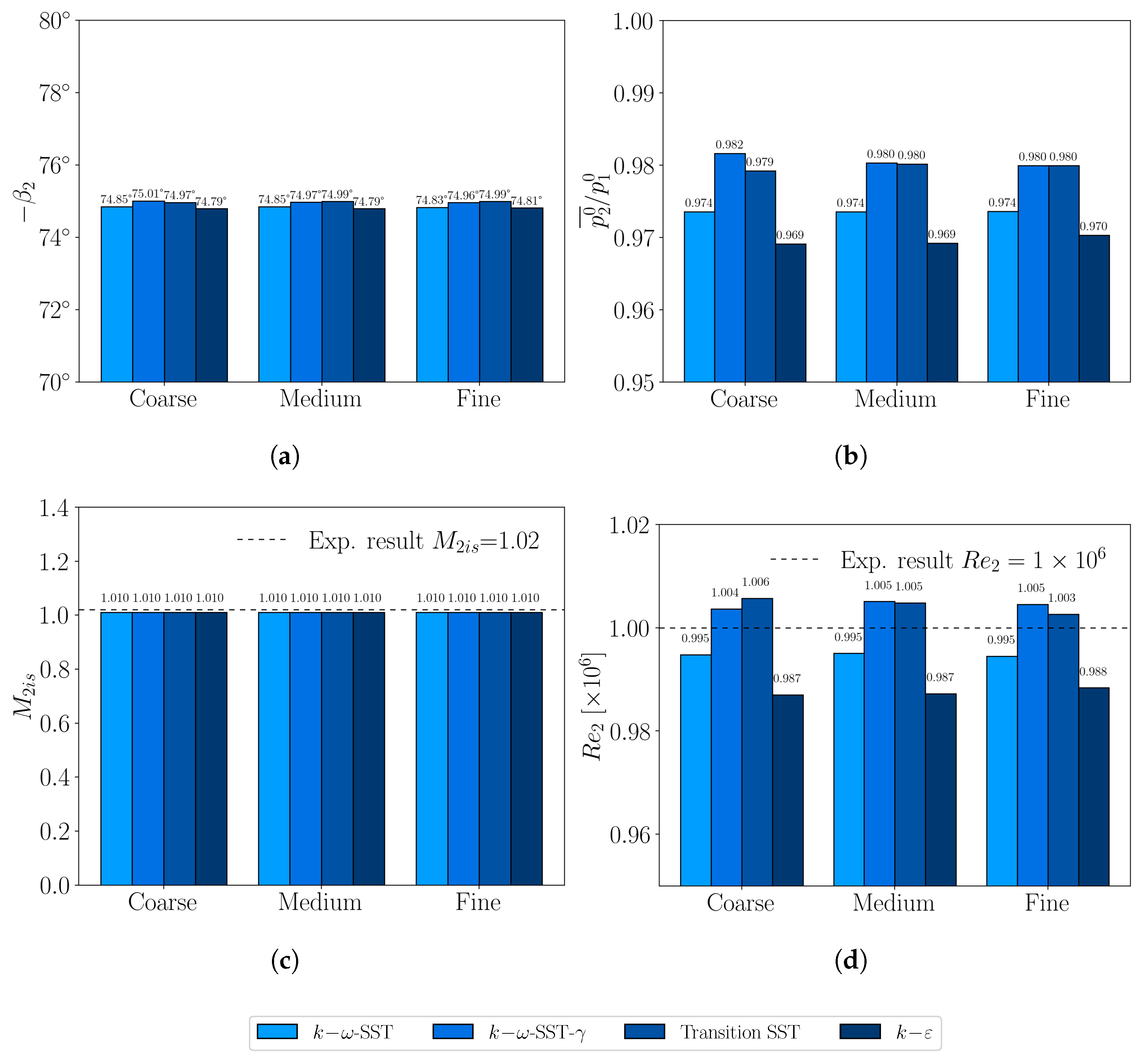
Global quantities are first analyzed to assess convergence behavior. Figure 2 reports the exit flow angle (Figure 2a), total pressure expansion ratio (Figure 2b), outlet isentropic Mach number (Figure 2c), and outlet Reynolds number R e 2 = ρ 2 u 2 c / μ 2 (Figure 2d) for the three mesh levels. All results are evaluated at the outlet through mass flow averaged quantities, defined as follows:
ϕ ¯ 2 = A 2 ρ u ϕ d A A 2 ρ u d A ,
where ϕ denotes the generic flow quantity, and A 2 is the outlet surface. The results indicate excellent agreement between the medium and fine meshes: the relative variation in the total pressure ratio is 0.0066%, while the exit angle differs by only 0.0045%. This confirms strong grid independence. Additionally, both the outlet isentropic Mach number and the outlet Reynolds number show good correlation with experimental data: the mean percentage deviation is 0.98% for M 2 , is and 0.663% for R e 2 , further confirming the mesh quality.

3.3.2. Near-Wall Quantities

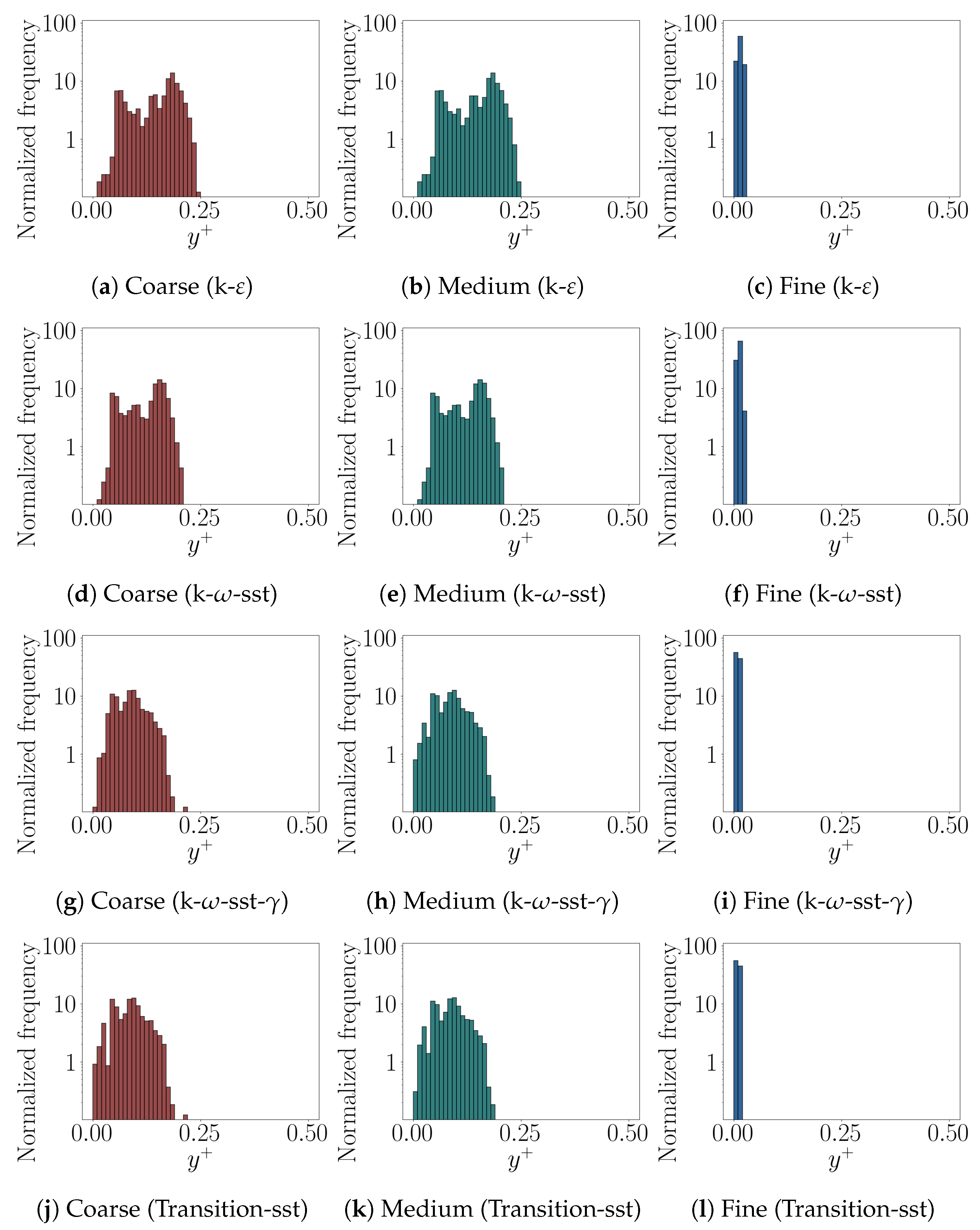
As a first step, near-wall resolution is verified via the normalized wall distance y + = ρ w u τ y w / μ w , where u τ = τ w / ρ w is the friction velocity and y w is the distance to the first cell center. Figure 3 presents y + -normalized frequencies for all turbulence models and mesh levels. The distributions confirm that even with the coarse and medium meshes, no values greater than 0.5 are detected, and the fine mesh reaches below 0.05. These results ensure accurate near-wall resolution, enabling low-Reynolds-number turbulence models to operate without wall functions. The difference between coarse and medium levels is minimal, as mesh refinement mainly targeted regions of shock interaction.
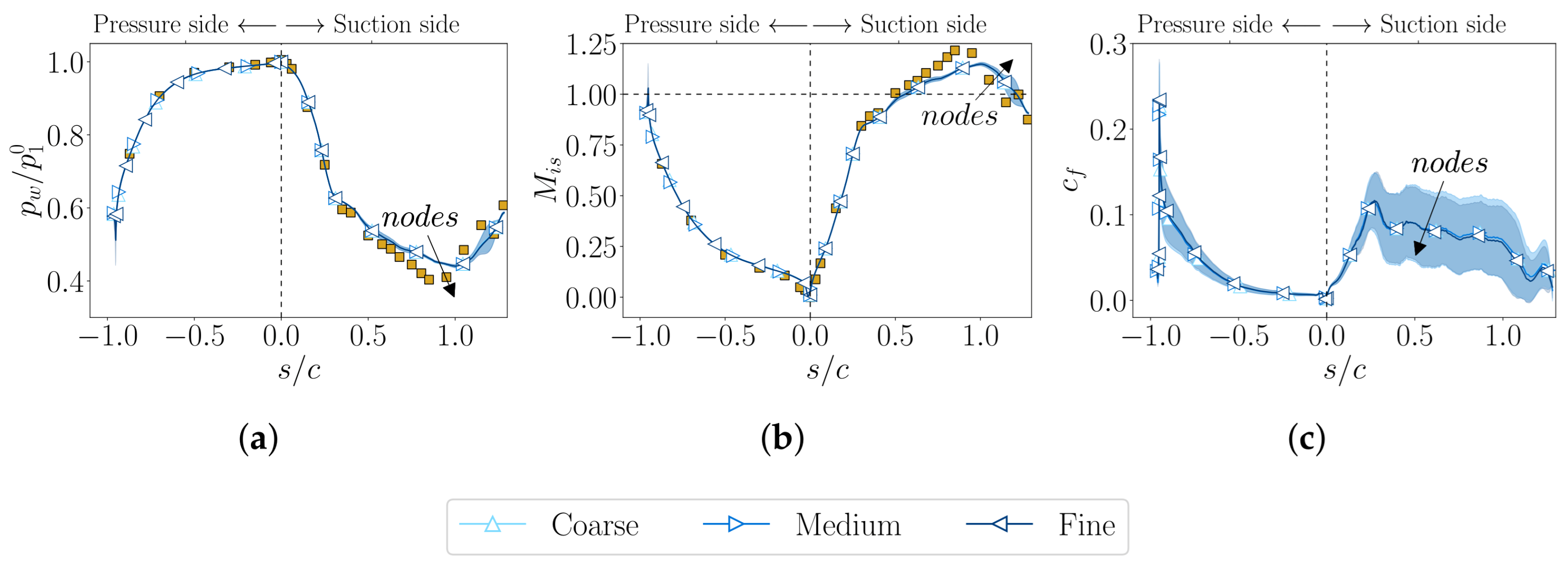
To further assess mesh sensitivity, several local wall quantities are examined. These include the wall static pressure p w , the local isentropic Mach number M is , and the wall friction coefficient c f , the latter defined as the non-dimensional ratio between the wall shear stress τ w and the inlet dynamic pressure q 1 = 1 / 2 ρ 1 u 1 2 :
c f = τ w 1 / 2 ρ 1 u 1 2
where τ w = μ w u / y is the wall shear stress, ρ 1 is the inlet density, and u 1 is the inlet velocity magnitude.
Given the variability among individual turbulence model predictions, a model-averaged response was employed to ensure a consistent basis for assessing grid convergence and subsequent analyses. The model-averaged response was obtained by combining the predictions from the turbulence models using a simple arithmetic ensemble mean. For each investigated quantity Q ( ξ ) , the results from all models were interpolated onto a common set of spatial or parametric coordinates ξ (e.g., chord-scaled curvilinear coordinate, s, or the pitchwise position in the wake, x / c a x ). The pointwise ensemble mean and standard deviation across the models were then computed as follows:
Q ¯ ( ξ ) = 1 N i = 1 N Q i ( ξ ) , σ Q ( ξ ) = 1 N i = 1 N Q i ( ξ ) Q ¯ ( ξ ) 2 ,
where N is the number of models, and Q i ( ξ ) is the prediction from the ( i -th model. The resulting mean profile Q ¯ ( ξ ) represents the model-averaged prediction, while the shaded envelopes shown in the figures correspond to σ Q ( ξ ) , quantifying the inter-model variability. This pointwise averaging procedure was applied consistently to all quantities (e.g., wall pressure, friction coefficient, wake losses), providing a uniform and unbiased measure of model-to-model uncertainty.
Figure 4 presents the comparison for all three mesh levels. The profiles are plotted along the normalized blade surface coordinate s / c , where s / c < 0 denotes the pressure side and s / c > 0 the suction side. Each curve represents the model-averaged prediction obtained from the ensemble of turbulence models, while the shaded regions indicate the corresponding inter-model envelope, bounded by the maximum and minimum values among individual models, thereby highlighting the modeling uncertainty associated with turbulence closure. Gold squares denote experimental measurements from Arts et al. [42]. As seen in Figure 4, no significant differences emerge between the three mesh levels for the isentropic Mach number and wall pressure distribution, confirming that discrepancies are primarily due to turbulence modeling rather than grid resolution. Conversely, more pronounced variations are observed for the wall friction coefficient c f , which is strongly influenced by the turbulence closure, underlining the model-dependent nature of near-wall shear stress prediction. Overall, the results demonstrate that mesh convergence is achieved for all key flow quantities except for c f , the accuracy of which is limited by the turbulence model rather than by the spatial discretization.
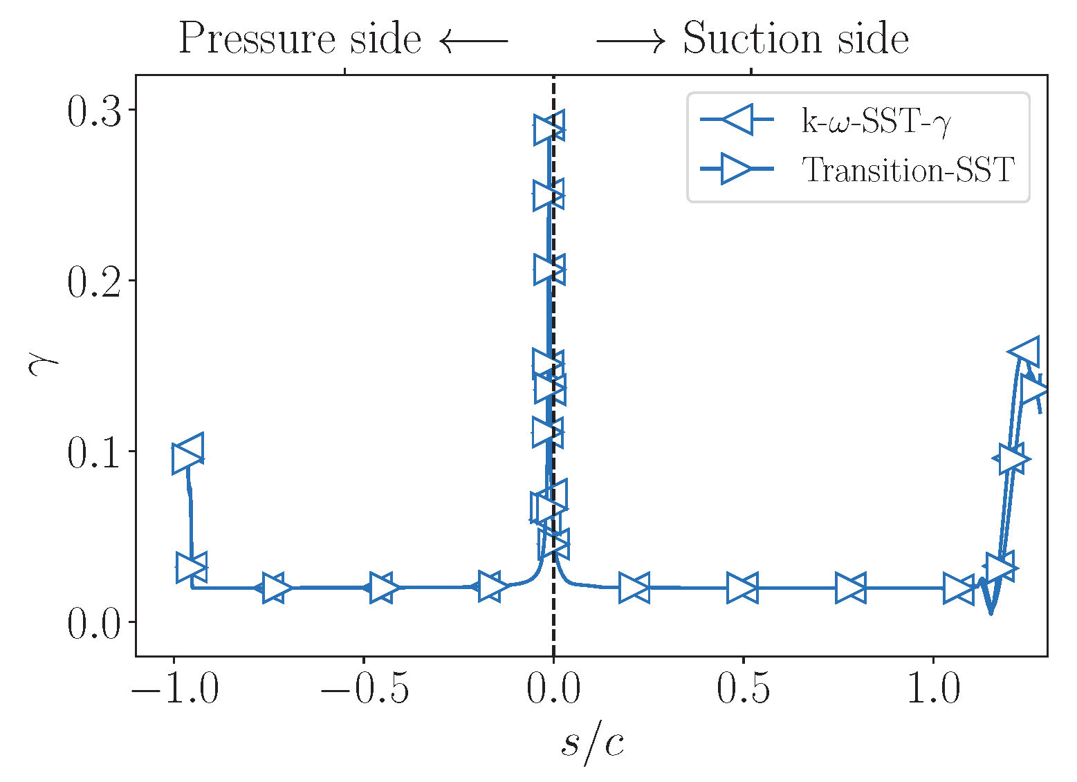
Finally, Figure 5 reports the predicted intermittency field γ along the blade surface, providing quantitative insight into the laminar-to-turbulent transition process. Intermittency is a key indicator of the transition state of the boundary layer, ranging from γ 0 in fully laminar regions to γ 1 in fully turbulent zones. Both turbulence models—k ω -SST– γ and Transition-SST ( γ R e θ )—produce qualitatively similar distributions. The intermittency remains close to 0.02 across the majority of the blade surface, with a localized peak near the leading edge ( γ 0.28 ) and a moderate rise at the trailing edge ( γ 0.14 ). These results suggest that the boundary layer remains predominantly laminar along most of the suction and pressure sides, with only partial transition developing in localized regions. This prediction is inconsistent with expectations for the Reynolds numbers considered in this cascade configuration, and highlights a common limitation of RANS-based transition modeling. In particular, the inability of such models to fully capture separation-induced transition or subtle instabilities in high-pressure turbine flows may lead to a misprediction of turbulence generation and associated aerodynamic losses.
However, based on the validation carried out, we strongly believe that no further action could improve the prediction of such flows within a RANS framework. Consequently, and in line with the grid-independence study, the medium-resolution mesh with 2 × 10 5 elements is adopted for all subsequent analyses, providing an effective balance between numerical accuracy and computational efficiency.

4. Results and Discussion

This section presents the comprehensive evaluation of the aerodynamic and thermal behavior of the flow, discussing the overall RANS database. The focus is placed on understanding the predictive capability of different turbulence closures and reducing the uncertainty associated with flow modeling of this configuration, in light of the objective to provide the community with a solid background about the setup associated with the LS89 test case.

4.1. Adiabatic Wall Arrangement

In the adiabatic configuration, simulations were performed at the three VKI operating points (MUR43, MUR45, and MUR47). Three turbulence closures were retained for the dataset k ω -SST, realizable k ε , k ω -SST– γ ; Transition-SST ( γ R e θ ) was used for mesh validation only and was not included in the database because it produced trends comparable to those of k ω -SST– γ .

4.1.1. Flow Qualitative Description

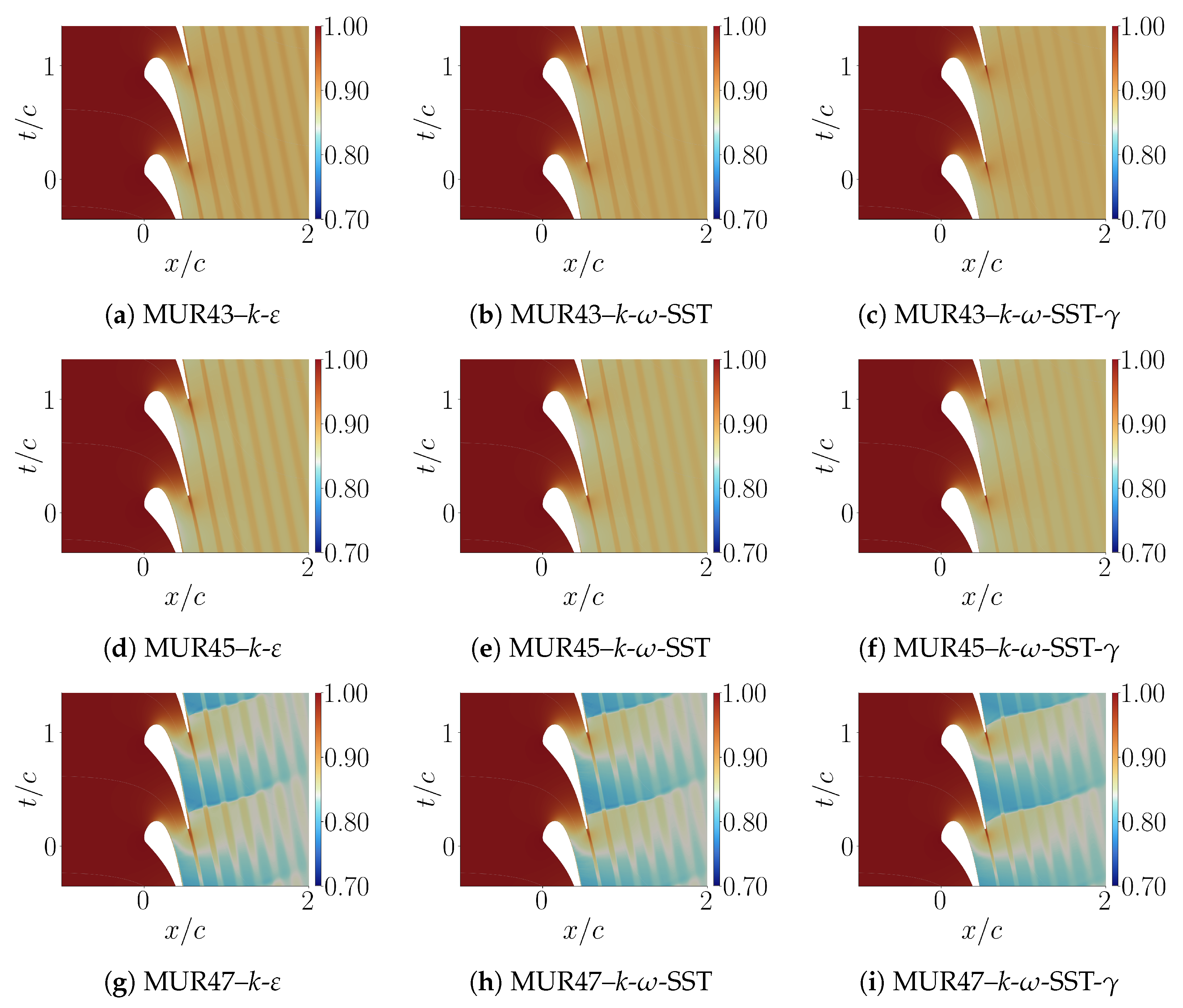
We first discuss the flow qualitatively. Figure 6 shows normalized static temperature contours ( T / T 1 0 ). All cases exhibit three distinct flow regions: an upstream region with nearly uniform temperature, a mid-passage zone with accelerating flow and cooling due to energy conversion, and a downstream wake region characterized by thermal and velocity deficits. At subsonic conditions (MUR43 and MUR45), the three turbulence closures yield qualitatively similar results, with mild differences in wake shape and temperature gradients. The wake remains diffuse, and the temperature decrease is gradual, indicating limited sensitivity to turbulence modeling in the absence of strong compressibility effects. For the transonic case, MUR47, stronger gradients and distinct features emerge. A sharper temperature drop and localized changes in gradient suggest the presence of shock waves, most evident in the k ε simulation. Shock location varies with the turbulence model: k ε predicts the shock to be closer to mid-chord, k ω -SST delays it slightly, and k ω -SST– γ pushes it further downstream, near the trailing edge. Finally, the wake in MUR47 appears wider, particularly in k ε .

4.1.2. Near Wall Quantities

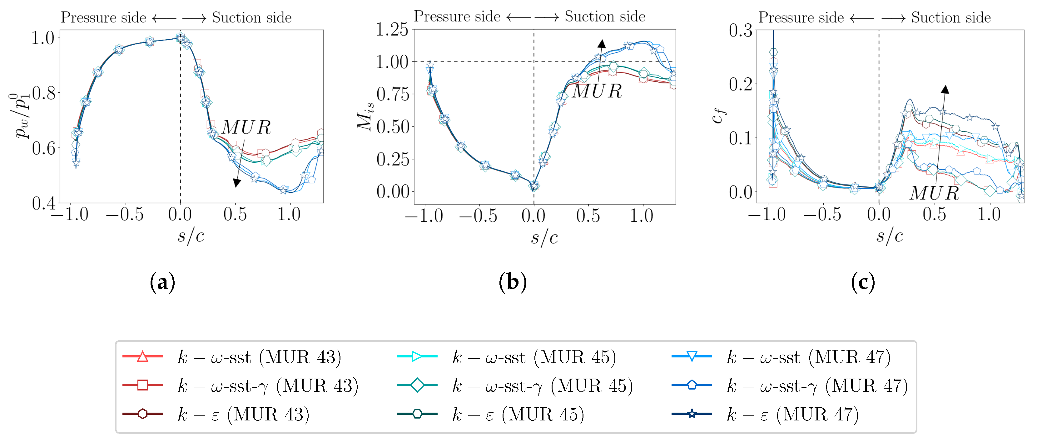
To quantify model differences, Figure 7 presents a comparative analysis of surface flow quantities—wall static pressure (Figure 7a), isentropic Mach number (Figure 7b), and wall friction coefficient (Figure 7c)—for all simulated MUR cases (MUR43, MUR45, MUR47) and three turbulence models (k ε , k ω -SST, and k ω -SST– γ ).
The static pressure distribution in Figure 7a reveals a consistent trend across all models and cases. The pressure side exhibits a gradual rise toward a maximum near the leading edge, followed by a sharp drop along the suction side. While minor differences arise between models, particularly on the suction surface, the overall agreement confirms the robustness of wall pressure predictions under varying modeling assumptions. The pressure plateau and minimum region on the suction side reflect the driving pressure drop responsible for accelerating the flow through the blade passage.
The isentropic Mach number profiles in Figure 7b capture the progressive acceleration over the suction side, with a peak near the trailing edge. The results for MUR43 and MUR45 are nearly indistinguishable, while MUR47 exhibits slightly higher acceleration, consistent with its increased outlet-to-inlet pressure ratio. Even for the isentropic Mach number, all turbulence closures yield similar qualitative features, with only moderate deviations in the location and magnitude of peak M is , which may be attributed to differences in boundary layer behavior and shock detection between models.
The wall friction coefficient, shown in Figure 7c, instead displays a stronger dependence on both the operating condition and turbulence model. On the pressure side, peak c f values are found near the leading edge due to stagnation and strong boundary layer gradients. On the suction side, a broad plateau is observed, with clear variations across models, particularly in MUR47 where shock–boundary layer interaction plays a prominent role. The k ε model predicts systematically higher friction levels. Conversely, the SST-based models provide smoother and lower c f distributions, with the k ω -SST– γ model offering further reductions due to its transition-sensitive formulation.
These results show that, across all MUR configurations, the wall pressure and isentropic Mach number are relatively insensitive to the turbulence closure, whereas wall shear stress predictions remain strongly model-dependent. To mitigate closure-related uncertainty, we adopt a pointwise model-averaging approach as in Equation (12). As discussed in previous analyses, none of the three considered turbulence closures emerges as consistently superior across all investigated conditions. While the wall pressure and isentropic Mach number predictions exhibit similar overall trends, the wall friction coefficient displays significant discrepancies across models, particularly under transonic flow conditions. Given this variability and the lack of a dominant model, a model-averaged response is adopted to reduce closure-specific bias and enhance robustness.
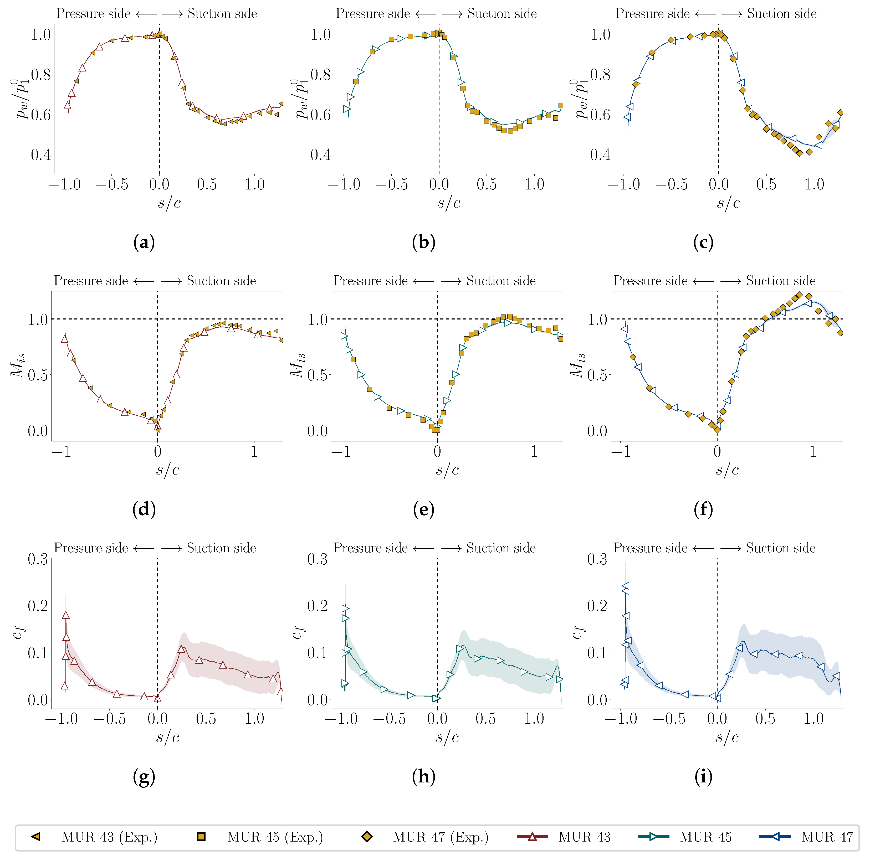
The averaged simulation results are shown in Figure 8, where the quantities are evaluated for each discharge Mach number case (MUR43, MUR45, MUR47). Specifically, Figure 8a–c depict the normalized wall pressure p w / p 1 0 ; Figure 8d–f show the isentropic Mach number M is ; and Figure 8g–i report the wall friction coefficient c f . Each profile is plotted as a function of the normalized surface coordinate s / c . Shaded regions indicate the prediction spread, and experimental data from [42] are included for comparison.
The agreement between RANS predictions and experimental pressure data is generally good. The standard deviation between simulation and measurements remains below 1.5% for the subsonic cases: 0.98% for MUR43 and 1.44% for MUR45. This value increases to 2.32% for MUR47, consistent with the increased difficulty of resolving shock–boundary layer interactions in the transonic regime. The aerodynamic behavior evolves significantly with increasing MUR. From Figure 8a–c, the suction-side pressure dip becomes deeper and the recovery stronger as the Mach number increases, highlighting more intense acceleration through the blade passage. Correspondingly, Figure 8d–f show that M is rises more steeply and peaks closer to the leading edge in MUR47, suggesting the presence of a shock wave. Although all models capture this behavior qualitatively, some mismatch in the shock location and intensity relative to those observed in experiments persists. The wall friction coefficient c f , shown in Figure 8g–i, reveals stronger model dependence and flow sensitivity. In MUR43 and MUR45, c f decreases along the suction side, reflecting gradual boundary layer development. However, for MUR47 (Figure 8i), c f flattens and stabilizes from s / c = 0.4 to s / c = 1.0 , indicative of a boundary layer thickened and stabilized by the stronger acceleration and delayed separation typical of transonic regimes. In all three MUR cases, the uncertainty band around the model-averaged profile is noticeably wide, reaching 20–30% of the mean value at the suction side, indicating that wall shear stress predictions are highly sensitive to the choice of turbulence closure. In summary, the model-averaged profiles provide a more reliable representation of the surface flow behavior, mitigating the impact of individual turbulence closure limitations and supporting more objective comparisons with experimental data, especially for transonic flow regimes where RANS closures are prone to diverging predictions.

4.1.3. Wake Characterization

One of the critical aspects in evaluating turbomachinery performance is the characterization of wake losses, which directly impact stage efficiency. Losses primarily originate from boundary layer separation, mixing, and turbulent dissipation in the wake region downstream of the blades and are generally measured as a total pressure drop. Associated quantities such as the total pressure deficit and the turbulent kinetic energy (TKE) offer valuable insight into the local aerodynamic degradation and the reliability of turbulence modeling strategies. In the context of compressible RANS simulations, TKE is defined as
k ˜ = 1 2 u 2 ˜ + v 2 ˜ + w 2 ˜ ,
which represents the mean kinetic energy per unit mass contained in the turbulent velocity fluctuations. It serves as a key indicator of turbulence intensity and the extent of energy redistribution caused by turbulent mixing in the wake.
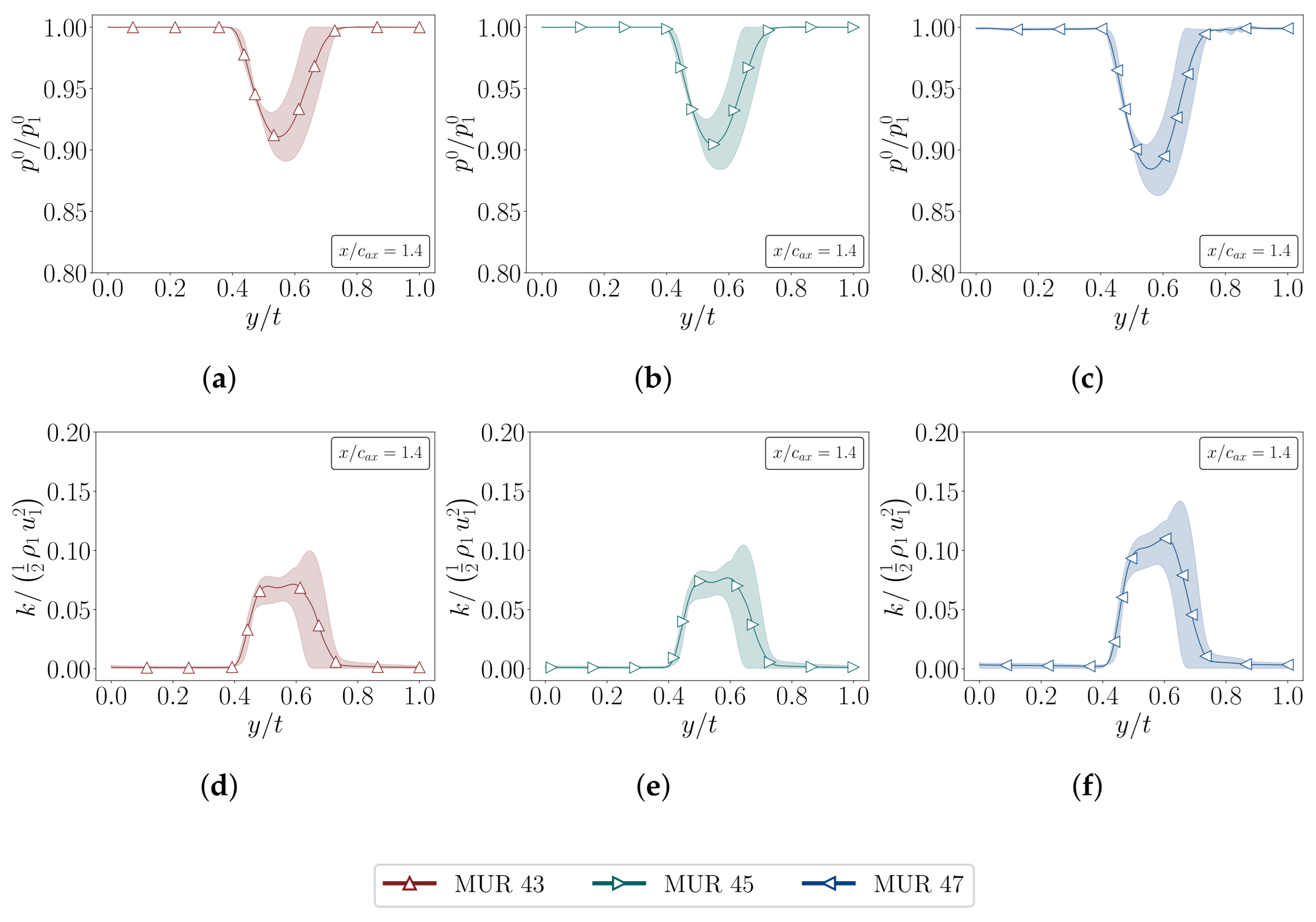
To assess these quantities quantitatively and provide additional insights for the present database, Figure 9 reports on the pitchwise distribution of total pressure loss and turbulent kinetic energy in the wake region at a normalized downstream location x / c ax = 1.4 for the three MUR conditions. Here, c ax denotes the axial chord length of the blade, defined as the projection of the blade chord c onto the axial direction: x / c ax = ( x / c ) sec ( γ s t a g ) , where c is the chord length and γ s t a g = 55 is the stagger angle of the blade. Figure 9a–c show the total pressure loss distributions for MUR43, MUR45, and MUR47, respectively, with p 0 / p 1 0 averaged over the three RANS models. The pressure deficit peaks at approximately y / t 0.6 , identifying the core of the blade wake. With increasing MUR, the depth and width of the pressure loss become more pronounced, consistent with intensified wake activity in transonic conditions. Figure 9d–f display the pitchwise distributions of turbulent kinetic energy for the same MUR cases. All cases exhibit a clear peak in TKE centered within the wake, corresponding to regions of high velocity gradients and turbulent production. Despite employing model-averaged RANS predictions with accompanying standard deviation bands, the underlying sensitivity to turbulence model selection remains clearly evident. In the wake region, even minor differences in boundary layer development and mixing intensity translate into substantial variations in both loss and turbulence predictions. Once again, we note that the uncertainty bands across the three cases are noticeably wide, with deviations reaching 25–35% in the suction-side shear layer, indicating a significant model-to-model spread in both p 0 / p 1 0 and TKE predictions. While all models reproduce the overall wake topology and the qualitative trends with increasing Mach number, their quantitative predictions differ substantially. The width of these bands highlights the strong sensitivity of wake mixing and dissipation to the turbulence closure, particularly in the core region and along the suction-side shear layer, where small differences in modeled turbulent transport lead to large variations in loss magnitude and wake thickness.

4.2. Diabatic Wall Arrangements

4.2.1. Flow Qualitative Description

After discussing the adiabatic wall arrangement, this section examines the influence of wall cooling on blade surface aerothermodynamics. The numerical setup varies the wall-to-recovery temperature ratio, T rat = T w / T r , between 1.0 and 0.5 to systematically assess thermal effects. The recovery temperature is defined as
T r = T 1 1 + γ g a s 1 2 P r l 1 / 3 M 1 2 ,
where P r l denotes the Prandtl number equal to 0.715. Reducing T w / T r introduces significant thermal gradients at the wall, which in turn affect boundary layer development, turbulence, and shock interactions. These conditions are representative of real turbine environments, where cooling strategies strongly influence aerodynamic performance.
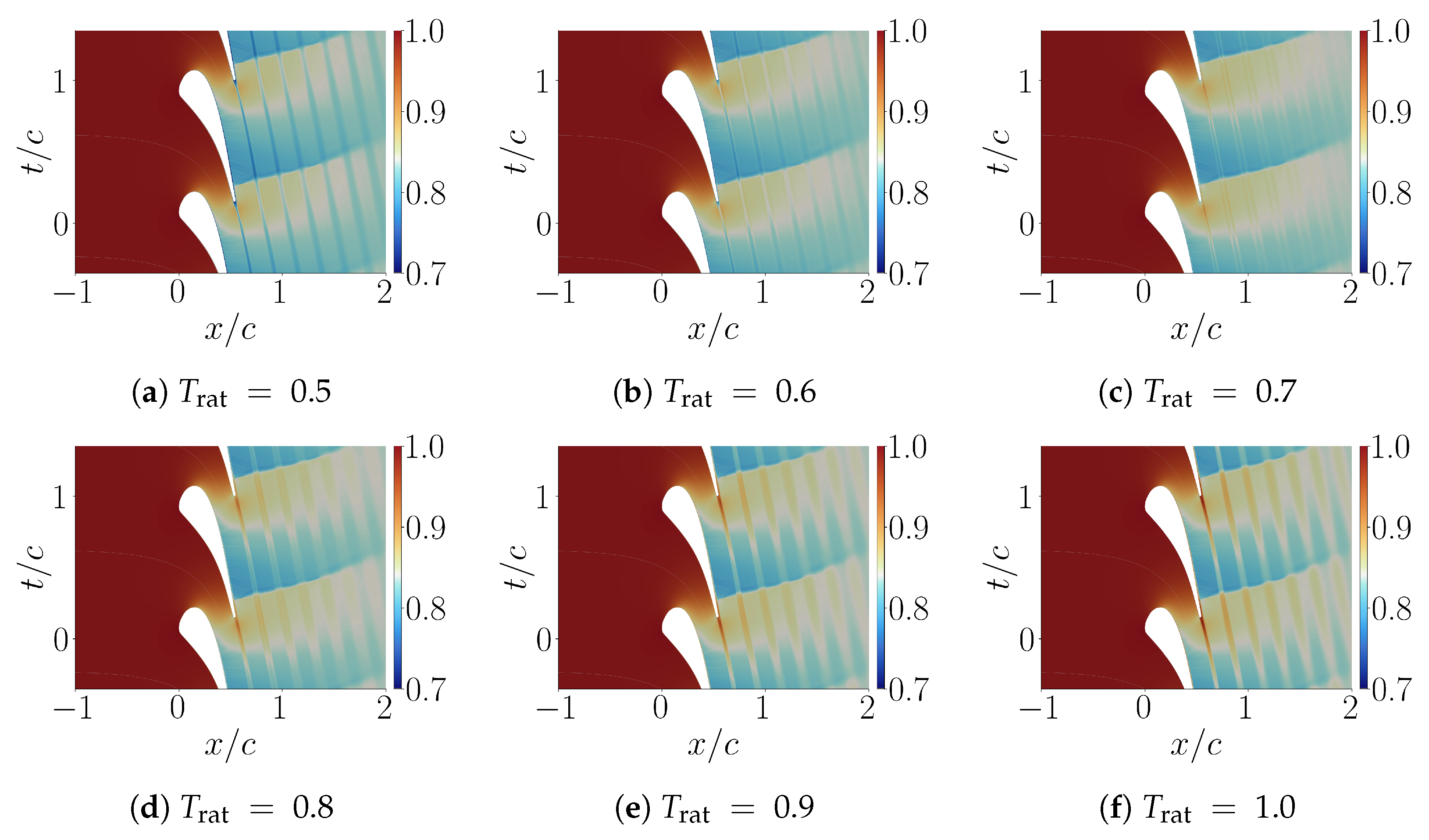
Starting with a qualitative perspective, Figure 10 illustrates the static temperature field over the blade surface for MUR47, computed using the k ω –SST model for different wall-to-recovery temperature ratios. As T rat decreases from Figure 10f to Figure 10a, progressive cooling of the wall region is evident, with increasingly steep temperature gradients localized near the surface. These gradients are particularly strong on the suction side, where flow acceleration and shock impingement exacerbate the local thermal contrast. At lower T rat values, the boundary layer exhibits a sharp temperature drop and visibly thinner thermal layers, which may influence local viscosity and, consequently, boundary layer development. In addition, cooling shifts the location and strength of thermal boundary layer separation and modifies the structure of oblique shock waves emanating from the blade surface. Lastly, as cooling increases, the regions of high thermal gradients migrate closer to the trailing edge, implying an upstream shift in the thermal footprint and its aerodynamic consequences. The influence of wall temperature also extends into the wake. As T rat decreases, the altered boundary layer development upstream modifies the thermal and momentum thickness feeding the wake. This results in a wake that becomes progressively narrower.

4.2.2. Near-Wall Quantities

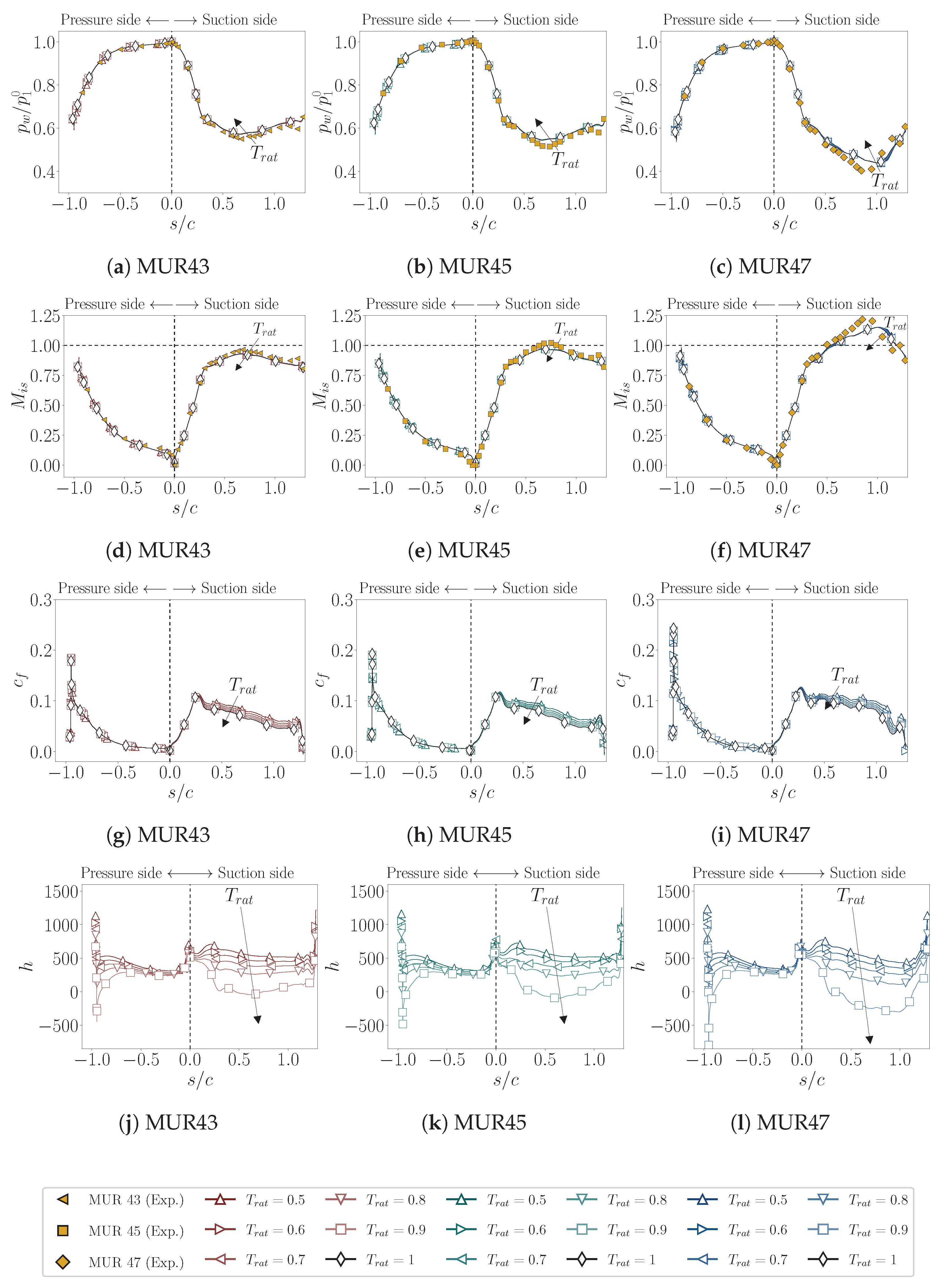
The near-wall aerodynamic and thermal quantities introduced in previous sections are now analyzed as a function of the wall-to-recovery temperature ratio. The quantities examined include the normalized wall pressure p w / p 1 0 , the isentropic Mach number M is , the friction coefficient c f , and the heat transfer coefficient.
h = q w T w T 1 .
Note that the heat transfer coefficient is not reported for the adiabatic case ( T rat = 1 ), since the denominator in the definition of h vanishes when T w T 1 , leading to undefined or non-physical values.
Figure 11a–c show the ensemble-averaged wall pressure distributions for MUR43, MUR45, and MUR47, respectively. For all cases, the wall pressure profiles display only mild sensitivity to the wall-to-recovery temperature ratio. The curves corresponding to different thermal boundary conditions remain largely superposed along both pressure and suction sides. This suggests that wall cooling has a limited influence on the global pressure field, which is primarily dictated by the inviscid core flow and the blade geometry. However, localized deviations are visible near the trailing edge on the suction side, especially for MUR47, where stronger cooling conditions slightly delay pressure recovery. These effects likely stem from cooling-induced shifts in boundary layer development and trailing edge separation.
The isentropic Mach number distributions, reported in Figure 11d–f, also exhibit a weak dependence on T rat . Across all Mach numbers, the curves remain close regardless of the cooling intensity, indicating that local flow acceleration and shock structures are not dramatically altered by thermal boundary conditions. Nevertheless, at higher Mach numbers (MUR45 and MUR47), small shifts in the peak suction-side Mach number suggest that cooling may subtly influence shock location and strength. These changes are consistent with slight modifications in the thermal boundary layer thickness, which indirectly affect compressibility effects and shock–boundary layer interactions.
A markedly different trend is observed for the skin friction coefficient, shown in Figure 11g–i. Here, the dependence on T rat is strong and monotonic. As the wall temperature decreases, c f increases significantly, particularly on the suction side. This behavior is attributed to the densification of the boundary layer that makes the velocity gradient steeper. The suction-side peak in c f , typically located downstream of the acceleration zone, shifts upstream and intensifies as cooling increases. The pressure side is less affected, except near the leading edge, where stagnation point heating can produce localized peaks.
Figure 11j–l display the distributions of the convective heat transfer coefficient, quantifying the local heat extraction from the flow. As expected, this quantity is highly sensitive to wall cooling. As T rat decreases, h rises substantially across both sides of the blade. The most intense heat transfer variation occurs on the suction side, particularly between s / c = 0.4 and s / c = 1.0 , where strong flow acceleration amplifies thermal gradients. The presence of shock waves near the trailing edge further modulates the distribution, creating localized peaks.
Overall, the results confirm that while wall pressure and isentropic Mach distributions are mostly insensitive to wall cooling, viscous and thermal boundary layer quantities such as c f and h exhibit a clear and nonlinear dependence on the thermal state of the cascade.

4.2.3. Wake Characterization

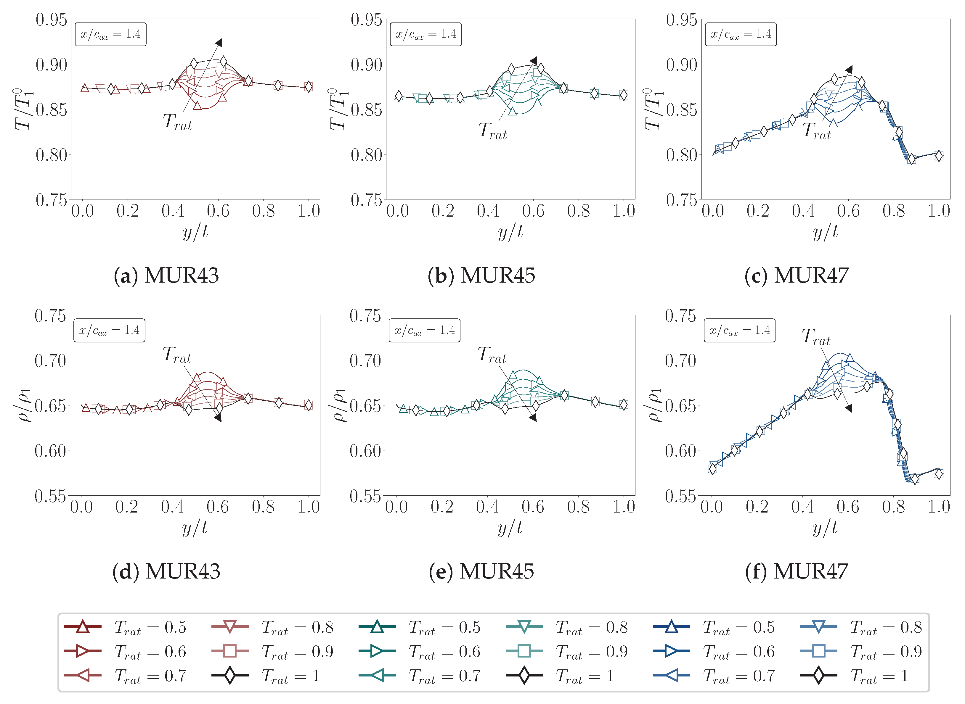
Figure 12 show the model-averaged pitchwise distributions of normalized static temperature ( T / T 1 0 ) and normalized density ( ρ / ρ 1 ), respectively, extracted in the wake at x / c ax = 1.4 . Quantities are plotted for all diabatic wall conditions and for the three Mach numbers investigated (MUR43, MUR45, MUR47).
Figure 12c reveals that the wake temperature profile exhibits a pronounced peak centered around y / t 0.5 as the wall-to-recovery temperature ratio T rat decreases. Lower wall temperatures lead to a narrowing of the wake profile, emphasizing a sharper peak, while higher wall temperatures tend to broaden the distribution into a more flattened plateau. This behavior reflects the impact of thermal boundary conditions on the extent and shape of the thermal wake deficit. In the outer irrotational region, i.e., outside the wake core ( y / t > 0.75 ), the influence of wall temperature on the thermal field becomes progressively weaker, proving RANS insensitive to the mixing process within the wake.
Figure 12d–f report on the corresponding density profiles in the wake. As expected, the density increases as the wall is cooled, due to the effect of reduced temperature. At lower Mach numbers, the density profiles are again flatter and broader, consistent with weaker cooling and more diffused wake characteristics. Interestingly, both temperature and density profiles tend to evolve toward bell-shaped distributions as T rat decreases, whereas higher wall temperatures result in broader and less pronounced gradients. This behavior reflects a stronger localization of thermal and inertial deficits in the cooled wake, with narrower and more distinct core structures. Overall, the results confirm that wall cooling has a strong impact on the wake region, while the irrotational flow remains essentially unaffected in the RANS solutions. This behavior highlights a clear limitation of RANS modeling, which underestimates sensitivity to mixing processes and therefore mispredicts the influence of wall cooling outside the wake.
Figure 12f presents the normalized density distribution extracted along the wake sampling line downstream of the blade trailing edge. Along this line, the profile exhibits a distinct local peak followed by a sharp decline, reflecting the characteristic evolution of the flow field across the wake. The initial density rise originates from the flow deceleration occurring within the wake core, where the velocity deficit induces a localized compression of the fluid. The subsequent steep decrease corresponds to the transition from this low-momentum region to the surrounding high-velocity irrotational stream, where rapid flow acceleration produces a pronounced density drop. Furthermore, the interaction with the downstream shock wave enhances this behavior: the pre-shock acceleration amplifies the density gradients observed immediately beyond the wake. The combined influence of wake-induced deceleration, flow re-acceleration, and shock–wake interaction explains the strong spatial variations captured in the normalized density profile.
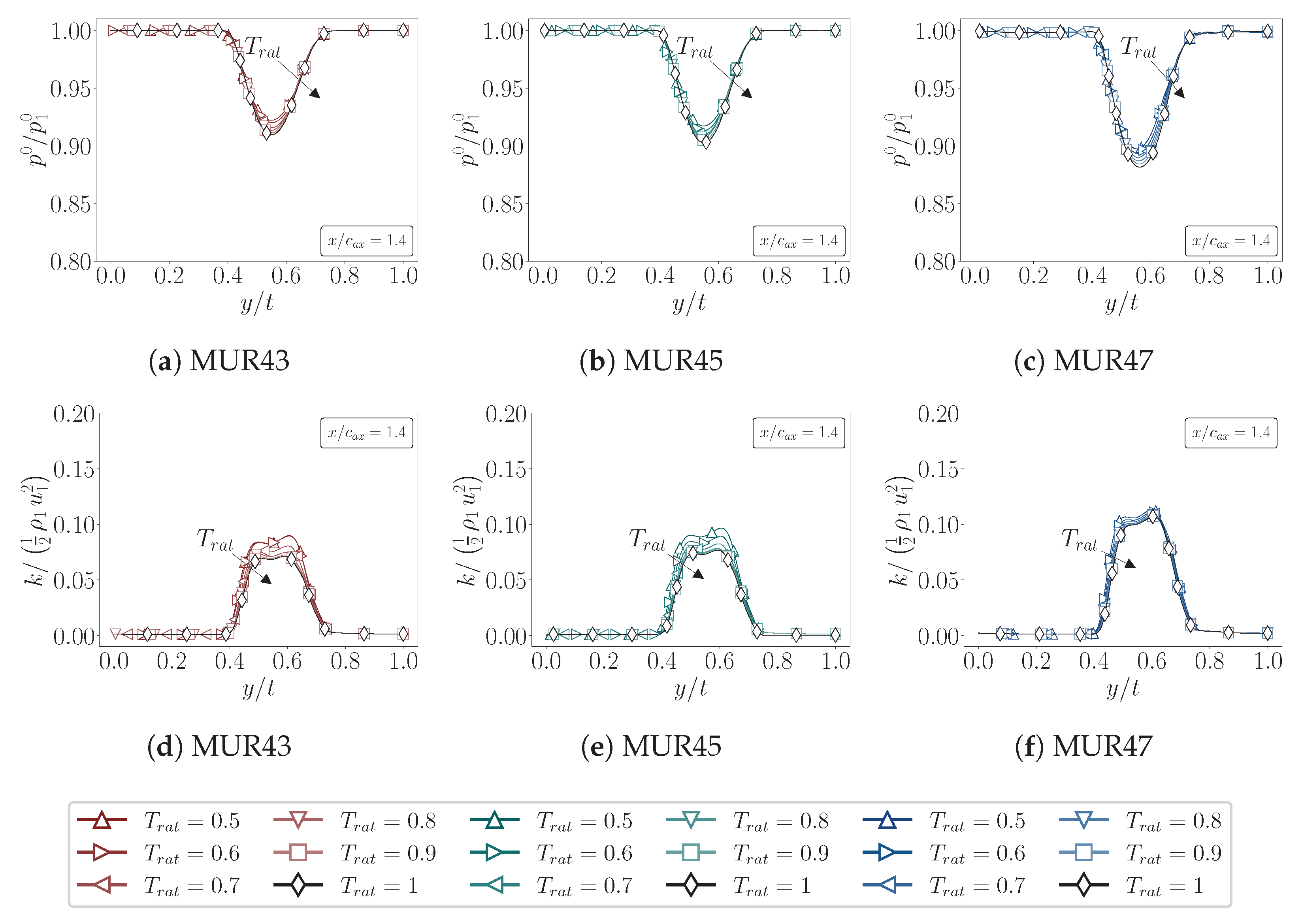
Figure 13 illustrates the impact of wall cooling at a streamwise location of x / c ax = 1.4 for the three MUR cases under diabatic conditions. The top row (Figure 13a–c) shows that increasing the wall temperature consistently produces a greater total pressure deficit in the wake. Conversely, the bottom row (Figure 13d–f) reveals an inverse behavior for turbulent kinetic energy, which decreases as the wall temperature rises. It is worth noting, however, that the RANS solutions display an unexpected behavior: turbulence levels increase with stronger cooling, whereas DNS and LES studies indicate that TKE should instead decrease as T rat is lowered, accompanied by a moderate rise in pressure losses De Vanna and Benini [43,44]. This discrepancy highlights a systematic limitation of RANS closures, which are typically calibrated for adiabatic wall conditions and thus fail to capture the correct interplay between wall cooling, turbulence production, and wake mixing.

5. Conclusions

The present study developed a comprehensive RANS-based aerothermal database of the LS89 transonic turbine cascade under both adiabatic and cooled wall conditions. The main findings can be summarized as follows:
  • A systematic mesh convergence analysis confirmed grid-independent solutions for global quantities, with near-exact agreement against experimental data for exit angle, outlet Mach number, and Reynolds number. Remaining discrepancies were primarily attributed to turbulence model dependence rather than discretization.
  • None of the considered RANS turbulence models consistently outperformed the others. To mitigate closure-induced variability, a model-averaging strategy was adopted, reducing uncertainty and providing more robust predictions, particularly for near-wall shear and wake quantities.
  • Wall pressure and isentropic Mach number distributions were shown to be largely insensitive to wall cooling, whereas viscous and thermal quantities (skin friction and heat transfer coefficients) displayed a strong nonlinear dependence on wall-to-recovery temperature ratio.
  • Wake characteristics, including total pressure deficit and turbulent kinetic energy, are strongly influenced by wall cooling at low Mach numbers, with colder walls deepening the pressure deficit and increasing turbulence intensity. Notably, the RANS solutions show an opposite trend to DNS/LES, predicting higher turbulence levels with stronger cooling, a discrepancy that reflects the limitations of closures calibrated primarily for adiabatic walls.
To support further research and benchmarking efforts, the complete RANS database discussed in the present work has been made openly available at “https://github.com/LS89-RANS-Data/LS89-RANS-data (accessed on 7 September 2025)”.
From a practical perspective, the present results provide useful guidance for both turbulence model development and turbine design. The comprehensive RANS-based aerothermal database developed herein serves as a reference for calibrating and validating turbulence models used in industrial applications, particularly for cooled turbine components operating in transonic regimes. Moreover, the proposed model-averaging strategy offers a robust framework for quantifying and reducing model form uncertainty, thereby enhancing the predictive reliability of RANS-based design tools.
Nevertheless, limitations of the present study must be acknowledged. First, the simulations were performed under steady-state conditions, which, while computationally efficient, neglect intrinsic unsteady flow dynamics that may influence turbine cascade performance, especially in transonic regimes. Second, the RANS framework, though effective for predicting time-averaged quantities, cannot capture the full turbulence spectrum or the detailed transition and shock–boundary layer interaction mechanisms that characterize real flows. Third, the employed RANS closures were originally calibrated for adiabatic or mildly heated wall conditions. Their application to strongly cooled surfaces may therefore lead to inaccurate predictions of turbulence production and wake development, as the underlying heat flux and near-wall modeling are not tuned for such diabatic regimes.
Future work should therefore aim to extend the present database using scale-resolving simulations, such as LES or DNS, to capture the unsteady and transitional phenomena unresolved by RANS. Such complementary datasets would enable more rigorous cross-validation and contribute to the development of next-generation turbulence models capable of reliably predicting complex aerothermal behavior in cooled, transonic turbine cascades.

Author Contributions

Conceptualization, F.D.V. and E.B.; methodology, D.F. and S.R.; software, D.F.; validation, D.F., S.R. and F.D.V.; formal analysis, D.F.; investigation, D.F.; resources, F.D.V.; data curation, D.F.; writing—original draft preparation, F.D.V.; writing—review and editing, D.F., S.R. and F.D.V.; visualization, D.F.; supervision, E.B. and F.D.V.; project administration, F.D.V. All authors have read and agreed to the published version of the manuscript.

Funding

This research received no external funding.

Data Availability Statement

The data associated with this study are openly available in the GitHub repository: “https://github.com/LS89-RANS-Data/LS89-RANS-data (accessed on 7 September 2025)”.

Acknowledgments

The authors gratefully acknowledge the Department of Industrial Engineering at the University of Padova for supporting this research within the framework of the ATLAS project (Advanced Turbine Operational Aerodynamics with Scale-Resolved Simulations).

Conflicts of Interest

The authors declare no conflicts of interest.

References

  1. De Vanna, F.; Benini, E. Impact of wall cooling on transonic gas turbine stators aerothermodynamics: Insights from Wall-Modeled LES. Appl. Therm. Eng. 2025, 272, 126396. [Google Scholar] [CrossRef]
  2. Bogard, D.G.; Thole, K.A. Gas Turbine Film Cooling. J. Propuls. Power 2012, 22, 249–270. [Google Scholar] [CrossRef]
  3. Bolaina, C.; Teloxa, J.; Varela, C.; Sierra, F.Z. Thermomechanical stress distributions in a gas turbine blade under the effect of cooling flow variations. J. Turbomach. 2013, 135, 064501. [Google Scholar] [CrossRef]
  4. Mukherjee, D. Stresses in Turbine Blades Due to Temperature and Load Variation. In Proceedings of the ASME 1978 International Gas Turbine Conference and Products Show, London, UK, 9–13 April 1978; American Society of Mechanical Engineers: New York, NY, USA, 1978; Volume 79726, p. V01BT02A057. [Google Scholar] [CrossRef]
  5. Sierra, F.Z.; Narzary, D.; Bolaina, C.; Han, J.C.; Kubiak, J.; Nebradt, J. Heat Transfer and Thermal Mechanical Stress Distributions in Gas Turbine Blades. In Proceedings of the ASME Turbo Expo 2009: Power for Land, Sea, and Air, Orlando, FL, USA, 8–12 June 2009; Volume 48845, pp. 115–126. [Google Scholar] [CrossRef]
  6. Colban, W.; Gratton, A.; Thole, K.A.; Haendler, M. Heat Transfer and Film-Cooling Measurements on a Stator Vane with Fan-Shaped Cooling Holes. J. Turbomach. 2005, 128, 53–61. [Google Scholar] [CrossRef]
  7. Andreini, A.; Caciolli, G.; Da Soghe, R.; Facchini, B.; Mazzei, L. Numerical Investigation on the Heat Transfer Enhancement due to Coolant Extraction on the Cold Side of Film Cooling Holes. In Proceedings of the ASME Turbo Expo 2014: Turbine Technical Conference and Exposition, Volume 5B: Heat Transfer, Düsseldorf, Germany, 16–20 June 2014; p. V05BT14A004. [Google Scholar] [CrossRef]
  8. Chi, Z.; Wang, L. Scale cooling–A novel fractal cooling structure for turbine vanes. J. Turbomach. 2025, 147, 061012. [Google Scholar] [CrossRef]
  9. Zhang, F.; Liu, C.; Wang, W.; Ye, L.; Li, B.; Liu, F. Film superposition prediction method for film cooling layouts with same opening ratio on the turbine blade. Appl. Therm. Eng. 2023, 233, 121105. [Google Scholar] [CrossRef]
  10. Bernardini, M.; Asproulias, I.; Larsson, J.; Pirozzoli, S.; Grasso, F. Heat transfer and wall temperature effects in shock wave turbulent boundary layer interactions. Phys. Rev. Fluids 2016, 1, 084403. [Google Scholar] [CrossRef]
  11. Kahveci, H.S.; Haldeman, C.W.; Mathison, R.M.; Dunn, M.G. Heat Transfer for the Film-Cooled Vane of a 1-1/2 Stage High-Pressure Transonic Turbine—Part I: Experimental Configuration and Data Review With Inlet Temperature Profile Effects. J. Turbomach. 2012, 135, 021027. [Google Scholar] [CrossRef]
  12. Kahveci, H.S.; Haldeman, C.W.; Mathison, R.M.; Dunn, M.G. Heat Transfer for the Film-Cooled Vane of a 1-1/2 Stage High-Pressure Transonic Turbine—Part II: Effect of Cooling Variation on the Vane Airfoil and Inner End Wall. J. Turbomach. 2012, 135, 021028. [Google Scholar] [CrossRef]
  13. Zhang, Q.; O’Dowd, D.O.; He, L.; Wheeler, A.P.S.; Ligrani, P.M.; Cheong, B.C.Y. Overtip Shock Wave Structure and Its Impact on Turbine Blade Tip Heat Transfer. J. Turbomach. 2011, 133, 041001. [Google Scholar] [CrossRef]
  14. Azad, G.S.; Han, J.C.; Teng, S.; Boyle, R.J. Heat Transfer and Pressure Distributions on a Gas Turbine Blade Tip. J. Turbomach. 2000, 122, 717–724. [Google Scholar] [CrossRef]
  15. Azad, G.S.; Han, J.C.; Boyle, R.J. Heat Transfer and Flow on the Squealer Tip of a Gas Turbine Blade. J. Turbomach. 2000, 122, 725–732. [Google Scholar] [CrossRef]
  16. Sampson, M.; Fairbanks, A.; Moseley, J.; Ligrani, P.M.; Xu, H.; Fox, M. Linear Cascade and Wind Tunnel Development for Turbine Blade Tip Heat Transfer Investigations With and Without Film Cooling. In Proceedings of the ASME Turbo Expo 2019: Turbomachinery Technical Conference and Exposition, Volume 5A: Heat Transfer, Phoenix, AZ, USA, 17–21 June 2019; p. V05AT13A007. [Google Scholar] [CrossRef]
  17. Giel, P.W.; Van Fossen, G.J.; Boyle, R.J.; Thurman, D.R.; Civinskas, K.C. Blade Heat Transfer Measurements and Predictions in a Transonic Turbine Cascade. In Proceedings of the ASME 1999 International Gas Turbine and Aeroengine Congress and Exhibition, Volume 3: Heat Transfer; Electric Power; Industrial and Cogeneration, Indianapolis, IN, USA, 7–10 June 1999; p. V003T01A029. [Google Scholar] [CrossRef]
  18. Chen, D.; Du, Q.; Xu, Q.; Xu, G.; Liu, H.; Li, H. Film cooling and aerodynamic loss performance of turbine vanes with fan-shaped and wave-trenched holes. Appl. Therm. Eng. 2023, 230, 120643. [Google Scholar] [CrossRef]
  19. Abuaf, N.; Bunker, R.; Lee, C.P. Heat Transfer and Film Cooling Effectiveness in a Linear Airfoil Cascade. J. Turbomach. 1997, 119, 302–309. [Google Scholar] [CrossRef]
  20. Tallman, J.A.; Haldeman, C.W.; Dunn, M.G.; Tolpadi, A.K.; Bergholz, R.F. Heat Transfer Measurements and Predictions for a Modern, High-Pressure, Transonic Turbine, Including Endwalls. J. Turbomach. 2009, 131, 021001. [Google Scholar] [CrossRef]
  21. Bianchini, C.; Andrei, L.; Andreini, A.; Facchini, B. Numerical Benchmark of Nonconventional RANS Turbulence Models for Film and Effusion Cooling. J. Turbomach. 2013, 135, 041026. [Google Scholar] [CrossRef]
  22. Ravelli, S.; Barigozzi, G. Comparison of RANS and Detached Eddy Simulation Modeling Against Measurements of Leading Edge Film Cooling on a First-Stage Vane. J. Turbomach. 2017, 139, 051005. [Google Scholar] [CrossRef]
  23. Jones, F.B.; Fox, D.W.; Bogard, D.G. Evaluating the Usefulness of RANS in Film Cooling. In Proceedings of the ASME Turbo Expo 2019: Turbomachinery Technical Conference and Exposition, Volume 5A: Heat Transfer, Phoenix, AZ, USA, 17–21 June 2019; p. V05AT12A019. [Google Scholar] [CrossRef]
  24. Rosafio, N.; Lopes, G.; Salvadori, S.; Lavagnoli, S.; Misul, D.A. RANS Prediction of Losses and Transition Onset in a High-Speed Low-Pressure Turbine Cascade. Energies 2023, 16, 7348. [Google Scholar] [CrossRef]
  25. Müller-Schindewolffs, C.; Baier, R.D.; Seume, J.R.; Herbst, F. Direct numerical simulation based analysis of RANS predictions of a low-pressure turbine cascade. J. Turbomach. 2017, 139, 081006. [Google Scholar] [CrossRef]
  26. Gourdain, N.; Gicquel, L.Y.; Collado, E. Comparison of RANS and LES for prediction of wall heat transfer in a highly loaded turbine guide vane. J. Propuls. Power 2012, 28, 423–433. [Google Scholar] [CrossRef]
  27. Marconcini, M.; Pacciani, R.; Arnone, A.; Michelassi, V.; Pichler, R.; Zhao, Y.; Sandberg, R. Large eddy simulation and RANS analysis of the end-wall flow in a linear low-pressure-turbine cascade–Part II: Loss generation. J. Turbomach. 2019, 141, 051004. [Google Scholar] [CrossRef]
  28. Denton, J.D. Some Limitations of Turbomachinery CFD. In Proceedings of the ASME Turbo Expo 2010: Power for Land, Sea, and Air, Volume 7: Turbomachinery, Parts A, B, and C, Glasgow, UK, 14–18 June 2010; pp. 735–745. [Google Scholar] [CrossRef]
  29. Huang, J.; Nicholson, G.L.; Duan, L.; Choudhari, M.M.; Bowersox, R.D.W. Simulation and modeling of cold-wall hypersonic turbulent boundary layers on flat plate. In Proceedings of the AIAA Scitech 2020 Forum, Orlando, FL, USA, 6–10 January 2020. [Google Scholar] [CrossRef]
  30. Borghi, M.R.; Spiegel, S.C.; Yoder, D.A.; Georgiadis, N.J.; Wernet, M.P. Turbulent simulations of cooling jets in crossflow. In Proceedings of the AIAA Scitech 2022 Forum, San Diego, CA, USA, 3–7 January 2022. [Google Scholar] [CrossRef]
  31. Pichler, R.; Zhao, Y.; Sandberg, R.; Michelassi, V.; Pacciani, R.; Marconcini, M.; Arnone, A. Large-Eddy Simulation and RANS Analysis of the End-Wall Flow in a Linear Low-Pressure Turbine Cascade, Part I: Flow and Secondary Vorticity Fields Under Varying Inlet Condition. J. Turbomach. 2019, 141, 121005. [Google Scholar] [CrossRef]
  32. Sandrin, S.; Mazzei, L.; Da Soghe, R.; Fontaneto, F. Computational Fluid Dynamics Prediction of External Thermal Loads on Film-Cooled Gas Turbine Vanes: A Validation of Reynolds-Averaged Navier–Stokes Transition Models and Scale-Resolving Simulations for the VKI LS-94 Test Case. Fluids 2024, 9, 91. [Google Scholar] [CrossRef]
  33. Hassan, J.S.; Yavuzkurt, S. Comparison of four different two-equation models of turbulence in predicting film cooling performance. In Proceedings of the ASME Turbo Expo 2006: Power for Land, Sea, and Air, Barcelona, Spain, 8–11 May 2006; Volume 4238, pp. 701–710. [Google Scholar] [CrossRef]
  34. BiAn, X.; Wang, Q.; Su, X.; Yuan, X. Interaction mechanisms of shock waves with the boundary layer and wakes in a highly-loaded NGV using hybrid RANS/LES. Chin. J. Aeronaut. 2020, 33, 149–160. [Google Scholar] [CrossRef]
  35. Heyse, J.F.; Mishra, A.A.; Iaccarino, G. Estimating RANS model uncertainty using machine learning. J. Glob. Power Propuls. Soc. 2021, 2021, 1–14. [Google Scholar] [CrossRef]
  36. Schobeiri, M.T.; Nikparto, A. A Comparative Numerical Study of Aerodynamics and Heat Transfer on Transitional Flow Around a Highly Loaded Turbine Blade With Flow Separation Using RANS, URANS and LES. In Proceedings of the ASME Turbo Expo 2014: Turbine Technical Conference and Exposition, Volume 5C: Heat Transfer, Düsseldorf, Germany, 16–20 June 2014; p. V05CT17A001. [Google Scholar] [CrossRef]
  37. Duraisamy, K.; Iaccarino, G.; Xiao, H. Turbulence Modeling in the Age of Data. Annu. Rev. Fluid Mech. 2019, 51, 357–377. [Google Scholar] [CrossRef]
  38. He, W.; Deng, Q.; Zhou, W.; Gao, T.; Feng, Z. Film cooling and aerodynamic performances of a turbine nozzle guide vane with trenched cooling holes. Appl. Therm. Eng. 2019, 150, 150–163. [Google Scholar] [CrossRef]
  39. Xiao, H.; Cinnella, P. Quantification of model uncertainty in RANS simulations: A review. Prog. Aerosp. Sci. 2019, 108, 1–31. [Google Scholar] [CrossRef]
  40. Edeling, W.; Cinnella, P.; Dwight, R.P. Predictive RANS simulations via Bayesian Model-Scenario Averaging. J. Comput. Phys. 2014, 275, 65–91. [Google Scholar] [CrossRef]
  41. Wang, J.X.; Sun, R.; Xiao, H. Quantification of uncertainties in turbulence modeling: A comparison of physics-based and random matrix theoretic approaches. Int. J. Heat Fluid Flow 2016, 62, 577–592. [Google Scholar] [CrossRef]
  42. Arts, T.; Lambert de Rouvroit, M.; Rutherford, A. Aerothermal Investigation of a Highly Loaded Transonic Linear Turbine Guide Vane Cascade. A Test Case for Inviscid and Viscous Flow Computations; VKI LS 1990-06; Von Karman Institute for Fluid Dynamics: Sint-Genesius-Rode, Belgium, 1990. [Google Scholar]
  43. De Vanna, F.; Benini, E. Wall-Modeled LES of a Transonic Gas Turbine Vane—Part I: Model Setup and Assessment of Turbulent Length Scales. J. Turbomach. 2025, 147, 111015. [Google Scholar] [CrossRef]
  44. De Vanna, F.; Benini, E. Wall-Modeled LES of a Transonic Gas Turbine Vane—Part II: Mach Number Effect and Losses Prediction. J. Turbomach. 2025, 147, 111016. [Google Scholar] [CrossRef]
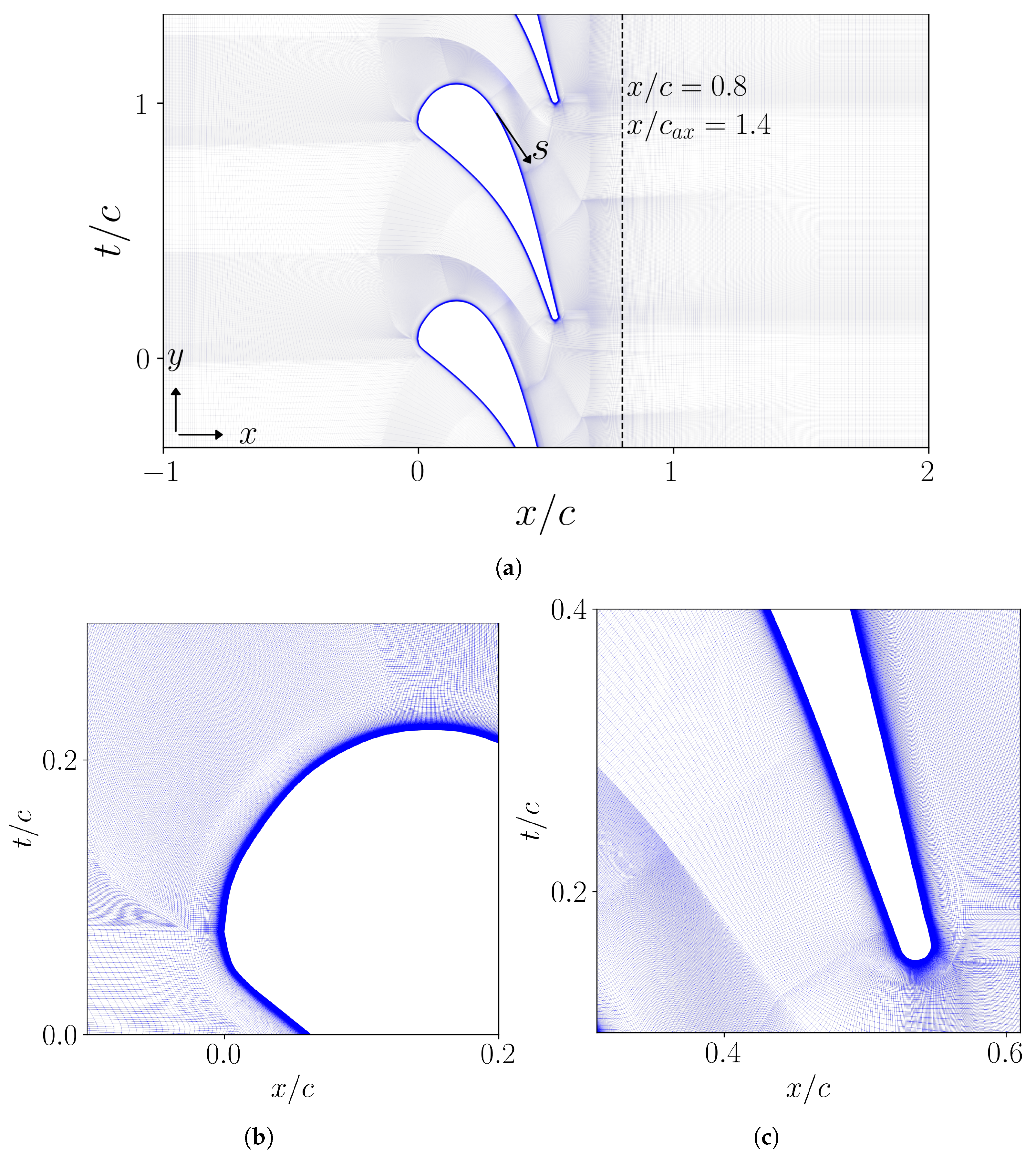
Figure 1. Computational mesh details. In (a), the global view of the computational grid is shown; the black dashed line refers to the location of the wake measurements, at x / c ax = 1.4 , consistent with the experimental setup of Arts et al. [42]. (b,c) provide close-up views of the leading edge and trailing edge mesh regions, respectively.
Energies 18 05321 g001
Figure 2. Mesh convergence analysis for global outlet parameters—exit angle (a), total pressure expansion ratio (b), isentropic Mach number (c), and Reynolds number (d).
Energies 18 05321 g002
Figure 3. Computed normalized wall y + on airfoil surface. Rows correspond to turbulence models; columns correspond to mesh refinement levels.
Energies 18 05321 g003
Figure 4. Mesh convergence of wall local quantities: static wall pressure distribution (a), isentropic Mach number (b), and wall friction coefficient (c). Shaded regions represent uncertainty from turbulence closure. Gold squares represent experimental data from Arts et al. [42].
Energies 18 05321 g004
Figure 5. Computed intermittency γ along the blade surface for the k ω -SST– γ model and the Transition-SST ( γ R e θ ) model. Results are based on the medium mesh ( 2 × 10 5 elements).
Energies 18 05321 g005
Figure 6. Static temperature distributions ( T / T 1 0 ) under adiabatic wall conditions. Each row corresponds to one of the three VKI operating conditions (MUR43, MUR45, MUR47), representing increasing outlet Mach numbers from subsonic to transonic regimes. Each column shows the results obtained with a different turbulence model: realizable k ε , k ω -SST, and k ω -SST– γ .
Energies 18 05321 g006
Figure 7. Comparison of wall pressure (a), isentropic Mach number (b), and wall friction (c) distributions across the three LS89 configurations (MUR43, MUR45, MUR47), and the three turbulence models: realizable k ε , k ω -SST, and k ω -SST– γ .
Energies 18 05321 g007
Figure 8. Comparison of simulation results with experimental data for the adiabatic configuration. (ac) show wall pressure distributions, (df) show the isentropic Mach number M is , and (gi) show the wall friction coefficients c f , across the three MUR cases. Shaded regions indicate the uncertainty range spanned by the different turbulence models, while solid curves represent the model-averaged response.
Energies 18 05321 g008
Figure 9. Pitchwise distributions of total pressure loss (ac) and turbulent kinetic energy (df) in the wake at x / c a x = 1.4 for the adiabatic wall condition across the three MUR cases. Curves denote the model-averaged predictions over the three RANS turbulence models, while shaded bands represent the inter-model deviation.
Energies 18 05321 g009
Figure 10. Static temperature contours over the blade surface for MUR47, computed with the k ω –SST model. Each panel corresponds to a different wall-to-recovery temperature ratio, T rat = T w / T r , ranging from 0.5 (a) to 1.0 (adiabatic, (f)).
Energies 18 05321 g010
Figure 11. Effect of wall-to-recovery temperature ratio on near-wall flow quantities for the three MUR cases: wall pressure (ac), isentropic Mach number (df), skin friction coefficient (gi), and heat transfer coefficient (jl). Results are shown for all T rat values, except for T rat = 1.0 in the heat transfer plots, where the definition becomes singular under adiabatic conditions. Lines denote model-averaged predictions (full uncertainty bands and individual model data are available in the public repository of the current study).
Energies 18 05321 g011
Figure 12. Pitchwise distributions of wake temperature (ac) and density (df) at x / c ax = 1.4 for diabatic wall conditions across the three MUR cases. Results represent model-averaged RANS predictions, with variations reflecting the influence of the wall-to-recovery temperature ratio (full uncertainty bands and individual model data are available in the public repository of the current study).
Energies 18 05321 g012
Figure 13. Pitchwise distributions of total pressure loss (ac) and turbulent kinetic energy (df) in the wake at x / c ax = 1.4 , under diabatic wall conditions and for all three MUR cases. All results are ensemble-averaged over the three turbulence models (full uncertainty bands and individual model data are available in the public repository of the current study).
Energies 18 05321 g013
Table 1. Geometrical parameters of the LS89 cascade from the experimental campaign of Arts et al. [42].
ParametersVariableValueUnit
Chordc67.647[mm]
Axial chord c a x 38.8[mm]
Stagger angle γ stag 55[°]
Pitcht57.5[mm]
Table 2. Simulation settings for the analyzed MUR cases. The pressure pairs reproduce the VKI LS89 operating points of Arts et al. [42].
Case p 1 0 [Pa] p 2 [Pa] T 1 0 [K] M 2 , is [−] Tu [%] μ t / μ [−]
MUR43143,50090,4054200.840510
MUR45147,50089,5834200.875510
MUR47159,60083,6614201.020510
Disclaimer/Publisher’s Note: The statements, opinions and data contained in all publications are solely those of the individual author(s) and contributor(s) and not of MDPI and/or the editor(s). MDPI and/or the editor(s) disclaim responsibility for any injury to people or property resulting from any ideas, methods, instructions or products referred to in the content.