Article

Heat Pump Optimization—Comparative Study of Different Optimization Algorithms and Heat Exchanger Area Approximations

Engineering Science and Technology IVT, UiT—The Arctic University of Norway, 9271 Tromsø, Norway
Energies 2025, 18(19), 5270; https://doi.org/10.3390/en18195270
Submission received: 31 July 2025 / Revised: 4 September 2025 / Accepted: 15 September 2025 / Published: 3 October 2025

Abstract

More energy efficient heat pumps can be designed if the industry is able to identify reliable optimization schemes able to predict how a fixed amount of money is best spent on the different individual components. For example, how to optimally design and size the different heat exchangers (HEs) in a heat pump with respect to cost and performance. In this work, different optimization algorithms and HE area integral approximations are compared for heat pumps with two and three HEs, with or without ejectors. Since the main goal is to identify optimal numerical schemes, not optimal designs, heat transfer is simplified, assuming a constant U-value for all HEs, which reduces the computational work significantly. Results show that high-order HE area approximations are 10 400 times faster than conventional trapezoidal and adaptive integral methods. High-order schemes with 45 grid points ( N ) obtained 80 100 % optimization success rates. For subcritical processes, the LMTD method produced accurate results with N 5 , but such schemes are unreliable and difficult to extend to real HE models with non-constant U. Results also show that constrained gradient-based optimizations are 10 times faster than particle swarm, and that conventional GA optimizations are extremely inefficient. This study therefore recommends applying high-order HE area approximations and gradient-based optimizations methods developing accurate optimization schemes for the industry, which include realistic heat transfer coefficients.

1. Introduction

Our research group has been focusing on the optimization of systems with heat exchangers (HEs), using real HE models based on detailed pressure drop and heat transfer calculations. However, it is difficult to identify the best HE designs and find the most cost-effective distribution of HE area between the different HEs. Hence, such studies are almost never done by industry or academia. The article by Rao et al. [1], named ‘Design optimization of heat exchangers with advanced optimization techniques: A review’, claims to be the first review work on parametric design optimization of HEs. However, Rao et al. only identified 98 referenced works, and concluded that most of them did not include detailed HE design optimization and typically applied old the cost models without a direct relation to the HE parts. Only seven parametric design optimization articles related to plate-fin HEs were identified. Optimization of systems with multiple HEs, with respect to cost and energy efficiency, will likely be an important tool, but better optimization schemes must be recognized before the industry will be able to make the transition for optimizing single HEs, to optimizing whole systems with multiple HEs. An end goal for this research is to develop a program that can optimize heat pump problems quickly and accurately. This is difficult, and a less ambitious goal is set here as a first step, i.e., to investigate and identify suitable optimization schemes, and to study the performance of new high-order HE integral methods introduced in the article by Brodal et al. [2]. The main research question is: ‘What are the best methods for optimizing system with multiple HEs’.
Heat pumps, refrigeration cycles and steam cycles are all examples of processes where both heat and work are important [3]. The energy efficiency of such processes is often increased the by adding more heat exchangers (HEs) to improve heat integration between hot and cold streams [4]. Identifying the best HE configuration in heat exchanger networks (HENs) involves solving mixed-integer optimization problems arising in a non-fixed process design [5]. Optimization of HENs via pinch analysis is often applied [6]. Some HEN problems only include HEs, but often also include other types of equipment [7]. The focus of this article is to study a few simple process optimization problems with a fixed process design, such as simultaneous heat integration (SHI) [8].
The cost and energy consumption of a process depend on the individual equipment, e.g., compressors, ejectors, expansion valves, and HEs such as evaporators, condensers, and gas coolers. The performances of compressors, turbines, and ejectors can be by isentropic efficiencies computed from external (inlet and outlet) values. HE performance can be described by the heat transfer area (A) and heat transfer coefficient (U). The HE area A is given by an integral, which can be solved using different approximations based on both external and internal HE values, i.e., the HE calculations involve additional internal points which increase the computational workload. Other equipment, such as compressors, turbines, ejectors, and valves, can be modeled exclusively from inlet and outlet values. Optimization can be used to identify the most energy efficient process with respect to cost and energy usage e.g., optimal pressures, temperatures, and refrigerant mixtures. The main idea is that different processes can be compared if they all have similar cost and operate with real equipment performance parameters and processes that are individually optimized. Systems with multiple HEs have previously often been optimized using simplified pinch point analysis to identify optimal refrigerant mixtures and heat pump processes configurations, see [9,10]. The basic assumption in such studies is that HEs operating with the same minimum temperature difference are similar in cost. However, this can be a highly inaccurate assumption, which cannot be used to find real optimal HE designs. The objective of this work is, therefore, to develop optimization schemes that can accurately identify both the most energy-efficient and the best equipment designs, e.g., to predict how a fixed amount of money is best distributed among the different HEs. It is typically considered too difficult to optimize multiple HEs simultaneously. Instead, the cost and design of each HE is often considered separately. Some process models already include detailed HE models suitable for optimizing custom-made HEs design one-by-one, such as HYSYS which is designed for modeling large oil and gas industry systems. Other industries operating with smaller non-custom-made HEs, e.g., commercial refrigeration and heat pump units, typically find suitable HE models from a supplier based on rough estimates, e.g., a 5 K temperature difference between the outlet streams in an evaporator. HE suppliers often provide computer programs such as SWEP SSP to assist the customers, and is, e.g., able to recommend a HE from a selection of SWEEP brand models for a given HE process.
Modelling a system with multiple HEs is complex and requires detailed knowledge about each HE, such as design, size, materials, and flow velocities. Hence, plate-fin and shell-and-tube HEs will require different heat transfer models, and condensers and evaporators have to be considered separately [11]. The literature review by Ayub et al. identified 22 different heat transfer models just for evaporation in plate HEs [12]. The review article by Eldeeb et al. describes 17 evaporation and 8 condensation models for plate HEs [13]. A comparison of 29 two-phase pressure drop and flow boiling heat transfer methods was conducted by Amalfi et al. [14]. The HE area A can be estimated by the logarithmic mean temperature difference (LMTD) approximation, which is an analytical expression describing true counter-current and co-current HEs processes where fluids have constant specific heat capacities cp. Hence, the conventional method is to extracted heat transfer correlations coefficients using LMTD integral approximations, e.g., done by Kruzel et al. [15] when studying boiling processes in shell-and-tube HEs, and by Szymczak et al. [16] when modeling a tube-in-tube condenser. Others such as Kumar et al. have used iterative LMTD and ∈-NTU methods [17]. Different methods have also been applied, e.g., Longo et al. develop heat transfer correlations to compute the HE area, based on trapezoid integral approximations using 100 grid points [18]. Accurate HE models often involve many internal HE points, i.e., additional fluid package calls to compute parameters such as viscosity, Prandtl number and conduction coefficients. HE calculations might also require iterative methods since heat transfer depends on pressure, while the HE pressure-drop depends on the heat transfer. Calculating accurate heat transfer and pressure profiles in optimization studies is therefore extremely time-consuming, which is perhaps the main reason why simpler HE models are typically used in large sensitivity studies. To reduce the computational load in this study, the optimization problem is simplified, i.e., assuming constant heat transfer (U-value) and zero pressure drop in all HEs. That is, the optimized processes studied here are not intended to model real optimal systems. The main goal is to identify the best numerical method, which can later be used to study processes with realistic HE models.
Optimization schemes consist of two main parts: the optimization algorithm and the process model. Finding the best combination is complex since several different optimization algorithms and HE area approximations can be applied. The implementation of fast and efficient numerical HE models is particularly important since such approximations require internal grid evaluations for each optimization step. Elias et al. combined pinch point temperature difference (ΔTpinch) and LMTD modeling to estimate HE area A and cost [19]. Watson et al. used LMTD method to model the overall thermal conductance of a HE, also known as the UA-value, and divided HEs into sections to improve accuracy of the calculations [20]. That is, five sections for single-phase and 20 for two-phase processes. Chen calculated A with higher accuracy by using an adaptive numerical step-size integration algorithm to improve the numerical approximation [21]. Adaptive algorithms are created to solve any integral using moderately high-order methods by dividing the problem into intervals where the parts likely to be inaccurate are divided into smaller intervals [22]. Numerical HE area integral estimates have conventionally been approximated using the trapezoidal rule, which is a low-order approximation, where the integral problem is divided into segments using equidistant grids, e.g., when modeling supercritical CO2 processes in brazed plate heat exchangers [23]. High-order methods are described by Hesthaven [24], and have been used for decades to solve smooth integrals since such problems requires fewer internal grid evaluations to obtain a given accuracy [22,25]. Hence, the smoothness of the HE data generated by fluid property packages, such as CoolProp [26], will be a decisive factor for the success of high-order integral methods, and need to be investigated. During pinch analysis of different systems, such as heat pump, refrigeration, LNG, CCS processes, it was discovered by the author that high-order interpolation methods improved pinch point calculations significantly [2]. High-order pinch point methods were also found to have performance advantages when used in optimization studies [27]. It has also been showed that high-order approximation generated much more accurate UA-values than conventional LMTD and low-order methods when modeling individual HEs [2]. However, it is not obvious if such high-order approximations also will improve optimization results related to systems with multiple HEs. The aim of the present study is to address this uncertainty.
The present study is limited to the optimization algorithms available in the [28] optimization toolbox, which includes conventional methods such as Fminsearch, Fmincon, Fminunc, genetic algorithm (GA) and particle swarm (PS). Fminsearch is an unconstrained method using a deterministic simplex algorithm [29]. Fmincon is also a deterministic method solving nonlinear constrained problems using gradients, which are calculated numerically using forward or central finite differences schemes. Fmincon uses either the interior-point method [30], or the sequential quadratic programming (sqp) method [31,32]. Fminunc is an unconstrained gradient-based method using the Quasi-Newton method [33]. Unlike the deterministic methods described above, GA and PS are stochastic algorithms. GA is inspired by genetics where traits from the most successful individuals are transferred to the next generation. GA includes strategies such as survival of the fittest, mutations and mixture of parents’ genes [34]. PS is unconstrained and based on assumption that the swarm members move and that their velocities are changed in each optimization step, depending on the best location of both the close neighbors and the whole swarm [35]. The article by Rao et al. concludes that gradient-based methods often fail compared to statistical optimization algorithms [1]. However, other process studies of systems including HEs have had great success with gradient-based optimization algorithms. For example, of the 186 LNG optimization articles identified in the review article by Austbø et al. [36], 15 were gradient-based using sqp algorithms [31,32], 29 used GA and 2 used PS.
It is important to identify faster and more successful optimization schemes which can be used by the industry to predict how a fixed amount of money is optimally spent on the different individual HEs, e.g., found in a heat pump. Real-world validation requires realistic heat transfer coefficients for all the different HEs. However, identifying heat transfer coefficients valid for all the different refrigerants and flow regimes is outside the scope of this numerical study, which compares different numerical methods to compute HE areas. Earlier studies have typically focus on finding optimal HE designs for a given process, and only a few have discussed different optimization algorithms, e.g., [1,36]. However, these studies did not discuss optimal process approximations. To the author’s knowledge, this is the first optimization study to simultaneously compare different optimization algorithms and HE area integral approximation. This is also believed to be the first optimization study using the high-order Chebyshev HE integration approximation recently suggested [2], and to suggest integral approximations using high-order Chebyshev differentiation matrixes. The main performance factors studied are optimization success rates and computer run times. Realistic optimization of all components in real heat pumps is difficult, and requires, e.g., optimization of individual HE design-parameters, such as the distance between plates, plate width, plate length, and plate thickness, while also optimizing how plates (HE area) should be distributed between the different HEs. Such schemes also need to compute realistic heat transfer, which is much more time-consuming since it require additional internal HE values, such as specific heat, mass density, flow velocity, and viscosity. In this study computer run-time is reduced significantly by only modeling simplified non-real heat transfer cases, assuming a constant U-value. The goal is to identify the best optimization algorithm and HE area approximation, which later can be used to optimize much harder real heat pump optimization problems, i.e., including realistic heat transfer coefficients, geometric designs, and cost models for each HE.

2. Materials and Method

This section presents a description of the modelling basis and the optimization approach for the heat pump processes studied.

2.1. Heat Pump Processes

Figure 1 shows flow diagrams of the three different heat pump designs optimized in this article. The feedwater HE is either operating as a gas cooler or a condenser, depending on operating conditions and the working fluid (refrigerant). The energy efficiency of a heat pump is described by the coefficient of performance (COP) defined as the ratio between the produced heat ( P h e a t ) and the compressor duty ( P c o m p ):
C O P = P h e a t P c o m p = h 2 h 3 h 2 h 1 ,
where h is specific enthalpy, using the numbering convention in Figure 1.

2.2. Process Modelling

Compressors, turbines, and ejectors are typically described by isentropic efficiency, which is to some extent related to the equipment cost, while expansion valves are assumed to be isenthalpic processes. Such equipment can be modeled using only inlet and outlet points in optimization studies, since the ejector performance can be implemented using optimization constraints [37]. HEs can also be modeled through optimization constraints but generally requires internal HE values. Unlike ejector constraints, HE constraints introduce numerical noise since they are based on numerical integral approximations. Process modeling is based on fluid property packages, which solves EOSs using numerical approximations. CoolProp is used in this study [26], and applies Ref. [38] for CO2, Ref. [39] for propane, Ref. [40] for ammonia and Ref. [41] for R134a.

2.2.1. Compressor and Ejector Performance

The compressor performance is modelled using isentropic efficiency:
η c o m p = P c o m p , i s P c o m p = h 2 , i s h 1 h 2 h 1 ,
where P c o m p , i s is the isentropic compression duty to pressure p 2 . The ejector is modeled with the ejector efficiency introduced by Elbel and Hrnjak [42]:
η e j e c t o r = m ˙ 6 ( h 8 , i s p 5 h 8 ) m ˙ 1 h 3 h 3 , i s p 5 .
That is, comparing the recovered work by the ejector with the maximum work recovered in an isentropic process. In other words, h 8 , i s p 5 and h 3 , i s p 5 are enthalpies modeled with isentropic processes from point 8 and 3, respectively, to the ejector outlet pressure p 5 . The optimal process, with an η e j e c t o r efficiency, is then found by expanding the optimization problem by adding the pressure ratio p r =   p 2 / p 5 as an optimization variable, while adding η m o d e l l e d   e j e c t o r     η e j e c t o r as an optimization constraint. Hence, the process ejector efficiency η m o d e l l e d   e j e c t o r must be calculated in each optimization step [37].

2.2.2. Modeling of HEs

All HEs are assumed to operate counter current with zero pressure drop, which is a common simplification, e.g., used by [43]. The mass flow of the refrigerant and the feedwater are calculated by the equations:
m ˙ R = P h e a t / ( h 2 h 3 )     and     m ˙ f e e d w a t e r = P h e a t / ( h b h a ) .
Optimal HE designs depend on the process and working fluids. When modeling HE performance, the heat transfer coefficient U is important. For processes with identical fluids, similar heat exchanger design and operating conditions, it is often reasonable to assume U = const. A general and accurate expression of U is difficult to derive, since it depends on flow velocities, film coefficients and material thermal conductivity. The internal temperature difference in which heat is transferred between the warm heat source and the cold heat sink ( T = T s o u r c e T s i n k ), is another important factor for the HE performance. The heat rate transferred between the fluids through a small part of the HE with heat transfer area d A , where T and U are approximately constant, is given as: d P     U · T · d A . The total HE area A is found by evaluating the integral:
A = 0 A d A = 0 P 1 U · T d P .
Such integral can be solved using several different approximations. There are many convection heat transfer models [12]. In this numerical study, the simplest model with a constant U value is investigated. Only positive T values are physically possible and a process with T = 0 will require an infinite HE area. Optimization algorithms are likely to create unphysical processes during the search, where the pinch point temperature difference T p i n c h =   min ( T ) is negative. To avoid errors in the HE area calculations when solving Equation (5), it is therefore important to include optimization constraints T p i n c h     > 0 for each HE. However, computing T p i n c h does not require much additional work, since all the T values required have already been calculated to find A . Also, optimized solutions typically have T p i n c h   >> 0, hence relatively inaccurate T p i n c h calculations will be sufficient to avoid unphysical temperature crossings in HEs. In this study, high-order interpolation methods have been used to calculate T p i n c h (see Ref. [2]).

2.2.3. HE Area Integral Approximations

The temperature difference T is a non-smooth function at bubble and dew points. To obtain intervals with a smooth T , each HE is divided into sections ( i ) separated by internal bubble and dew points. It is also possible to divide these sections into smaller sections. The heating duty of section i is: P i = m ˙ s o u r c e · h s o u r c e , i , where h s o u r c e , i is the difference between the inlet and outlet enthalpies of the heat source for section i . The heating ratio P i / P is used to distribute N grid points evenly over the different sections, and the number of grid points in section i is named N g r i d , i . The internal specific enthalpies, of the heat sink and heat source fluids in a HE section ( i ), are given by the linear transformations:
h s o u r c e , i j = x i j + 1 2 · P i m ˙ s o u r c e +   h s o u r c e , i , 1 and   h s i n k , i j = x i j + 1 2 · P i m ˙ s i n k +   h s i n k , i , 1 .
The specific enthalpies h s o u r c e , i , 1 and h s i n k , i , 1   at the first grid point in each HE section can be calculated with CoolProp directly. The heating power formula: P i j = m ˙ s o u r c e · h s o u r c e , i j h 2 , is then used to compute h at each grid point. Since both pressure and the enthalpy are known at each grid point, the temperatures T s o u r c e , i j and T s i n k , i j can be calculated using CoolProp, and the temperature difference at this HE grid point is:
T i j = T s o u r c e , i j T s i n k , i j ,
If the U -value is known at each grid point, the HE area integral in Equation (5) can be solved numerically.
Analytically Approximation (‘LMTD’)
The LMTD model is derived analytically for HE with pure parallel (co-current or counter-current), where fluids have constant specific heat c p during heat transfer, i.e., d P   m ˙ · c p · d T . The simplest LMTD approach, which is probably the most conventional method, only considers temperatures at the heat exchanger end-points. However, this model can improve accuracy by including internal points also. That is, divide the HE into smaller elements using equidistant distributed grids, and calculate the heat transfer area for each element using the values at neighboring grid points ( j and j 1 ) for each section i . This method is here named ‘LMTD’, and therefore calculates the total transfer area as the sum of each HE area part:
A = 0 P 1 U · T d P i j = 2 N g r i d , i l n T i j T i j 1 T i j T i j 1 · P i j P i j 1 U ¯ i j ,
where U ¯ i j is the average value between node j 1 and node j in element i . Note that, U ¯ i j = U in this study, since U is assumed to be constant. Note that this approximation therefore is less accurate when modeling systems with a non-constant U -value.
Low-Order Approximation (‘Trapezoidal’)
The integral problem in Equation (5) can be solved numerically using standard trapezoidal rule, which is a 2nd-order integral approximation:
A i j = 2 N g r i d , i 1 2 ·   1 U i j · T i j + 1 U i j 1 · T i j 1   · P i j P i j 1 .
Equidistant distributed grids are used, given by the formula:
x i j = 1 + 2 · j 1 N g r i d , i 1 ,   for   j = 1 , , N g r i d , i .
High-Order Approximation (Base Case)
A high-order (spectral) interpolation scheme can also be applied to solve integrals, e.g., using Chebyshev grid nodes x i defined as:
x i j = c o s π · j 1 N g r i d , i 1 ,   for   j = 1 , , N g r i d , i .
Such points cluster at the ends, which is important feature for high-order interpolation schemes [25]. Chebyshev integral weights w i ( j ) and values at the Chebyshev grid nodes x i j can then be used to compute a high-order approximation of the integral in Equation (5):
A = 0 P 1 U · T   d P = 1 1 d P d x · 1 U · T   d x i j = 1 N g r i d , i P i N g r i d , i P i 1 2 · w i j U i j · T i j .
High-Order Alternatives
Integral and derivation are inverse functions, and the integral can therefore also be solved using a differentiation matrix. The MATLAB function ‘ g a l l e r y ’ (in MATLAB version R2020a) is used to calculate the N g r i d , i   ×   N g r i d , i spectral differentiation matrix D i from an analytical expression, derived from the behavior of Chebyshev polynomials [24,25]. In order for the integral value to start at zero at the first node point, the spectral differentiation matrix is modified in the MATLAB script writing ‘D(1,:) = 0’ and ‘D(1,1) = 1’, as explained by Trefethen [25]. The integral is then computed as:
A = 0 P 1 U · T   d P = 1 1 d P d x · 1 U · T   d x i P i N g r i d , i P i 1 2 · i n v ( D i ) · f i ,
where the elements of the vector f i is: f i j = 1 / ( U i j · T i j ). This approximation is here named ‘high-order: inv(D)*f’. Note that MATLAB recommend solving such problems with the matrix backslash operator [28], which solves inverse problems with LU factorization or a least squares solver [44], depending on the condition number of D matrix. If the matrix backslash operator, the HE area approximation is named ‘high-order: D/f’.
Semi High-Order Approximation
This scheme divides HE sections into smaller ones, reducing the order of the integral approximation. The ‘High-order’ method is applied to all the smaller section, creating semi high-order scheme where elements have fewer grid points. A scheme operating with maximum 8 grid points in each HE section is named ‘Semi4–8’, since such sections will have 4   N g r i d , i   8 grid points. That is, a high-order (Base Case) section with 9 grid points is divided into two sections with 4 and 5 grid points.
Adaptive Semi High-Order Approximation
Adaptive algorithms divide sections identified as problematic into smaller intervals [22]. This approach is tested by using the built in MATLAB function ‘integral’ to compute Equation (5).

2.3. Optimization

The aim is to identify the most energy efficient heat pump configuration ( C O P o p t i m i z e d ) for a given cost. However, implementing accurate cost models are outside the scope of this article, where all equipment costs are assumed to be fixed. That is, assuming a fixed combined HE cost. The heat transfer area A is calculated for each HE, i.e., the evaporator ( A e v a p o r a t o r ), gas cooler ( A g a s   c o o l e r ) and internal HE ( A I H E ). The problem is further simplified by assuming that the combined HE area A t o t = A e v a p o r a t o r + A g a s   c o o l e r + A I H E is directly related to the combined HE cost. Hence, the optimization finds the best heat pump with a maximum allowed combined HE area A m a x , where A t o t A m a x is an optimization constraint. Constant compressor and ejector efficiencies ( η c o m p and η e j e c t o r ) are used to model constant equipment cost in this optimization study. Since optimization algorithms find a minimum, the optimization problem becomes:
C O P o p t i m i z e d = min C O P ,   for   all   processes   with   A t o t A m a x .
The main goal is to identify fast and successful conventional optimization algorithms offered in the MATLAB Optimization Toolbox. Unless stated, default MATLAB Optimization Toolbox optimization parameters are used. The constrained gradient-based Fmincon method is modeled with either forward and central finite differences schemes, while using interior-point [30] or sequential quadratic programming (sqp) algorithms [31,32]. These are titled ‘Fmincon(sqp,forward)’, ‘Fmincon(sqp,cetral)’, ‘Fmincon(interior,forward)’ and ‘Fmincon(interior,central)’. GA is modeled using population size 50, and the results are named ‘GA(50)’. PS is modeled with both 10 and 50 swarm sizes, labeled ‘PS(10)’ and ‘PS(50)’, respectively.

Optimization Scheme

Process performance data, such as COP, ejector efficiency ( η m o d e l l e d   e j e c t o r ), T p i n c h in HEs and HE areas A , are calculated in each optimization step. The process model requires inputs directly defined in the case study, but also the optimization variables x . For example, x = [ T 1 , T 3 , p 2 ] for ‘Heat pump A’. That is, the optimization assumes that the back pressure valve is adjusting the back pressure ( p 2 ) to obtain optimal COP. The evaporator outlet temperature ( T 1 ) and condenser outlet temperature ( T 3 ) are determined by the size and geometry of the evaporator and condenser, respectively. However, the optimal size and geometry of the individual HEs in the heat pump depend on each other if the combined cost (or HE area) is assumed fixed. Hence, the optimization identifies the optimal combination of T 1 and T 3 through optimization constraints. Heat transfer also depends on HE geometry, and the performance of a plate HE depends on parameters such as distance between plates, plate width, plate length and plate thickness. Note that all these parameters are known for a specific HE model provided by a retailer, however, such parameters can also be optimized to find an optimal custom made HE design, but this is more difficult to optimize since this will require more optimization variables, i.e., x must include additional geometric HE design-parameters. It is also more difficult to find a set of heat transfer coefficients valid for all possible HE designs, compared to optimizing a retailer HE model, where heat transfer coefficients have already been obtained from experiments. Table 1 shows the initial optimization points ( x 0 ) used for all cases. A small random noise is added to the initial point, using the MATLAB function ‘rand’, to avoid identical optimization results for all systems solved with highly accurate HE models. The lower and upper optimization bounds are only used by GA and PS. To speed up GA and PS algorithms the MATLAB settings ‘InitialPopulationMatrix’ and ‘InitialSwarmMatrix’ are used, respectively, with a shotgun algorithm that distributes initial points randomly in the region: [ x 0 · 0.95, x 0 · 1.05]. Input and output parameters in the process and optimization schemes are shown in Table 2 and Table 3.
Ejectors are modeled with a maximum allowed ejector efficiency optimization constraint: η m o d e l l e d   e j e c t o r   η e j e c t o r . Other optimization constraints are implemented to ensure realistic heat pump processes, e.g., to avoid temperature crossings in HEs ( Δ T p i n c h   e v a p o r a t o r 0 , Δ T p i n c h   g a s   c o o l e r 0 and Δ T p i n c h   I H E 0 ), pressure increase in expansion valves ( Δ p v a l v e 0 ) and temperature reduction in suction gas heaters ( T 3 T 3 * 0 ). Systems with ejectors are also modeled with additional constraints requiring the mass flows to be positive.
Of the optimization methods investigated here, only Fmincon has a direct implementation of the nonlinear constraints. Fminsearch, Fminunc, GA and PS are unconstrained methods, and are solved using penalty terms, e.g., the constraint A t o t   A m a x , is implemented as:
C O P o p t i m i z e d = m i n ( C O P + k · max 0 , A t o t A m a x 2 )
where the penalty factor k = 1000 is used. All the other nonlinear optimization constraints are implemented using the same penalty factor. Constraint violations in optimized results can be an indication that the optimization failed, and that the system therefore should be reoptimized. In this study, only optimizations with a b s ( A t o t A m a x )     0.001 m2 are considered successful. However, the real constraint violation can be much greater if the A t o t estimate is inaccurate.

2.4. Error Estimates, Run Time, and Definition of Failed Cases

The optimization has failed if the result violates the default MATLAB optimization tolerances or the user defined constraint tolerance: | A t o t A m a x |   >   0.001 m2. Such cases must be reoptimized and are therefore given the MATLAB-value ‘not a number’. Since an analytical solution of the optimal heat pump configuration is not available, the best COP value, C O P o p t i m a l   =   m a x ( C O P o p t i m i z e d ) , is estimated from all the optimization algorithm results with high-order HE area approximations and N = 100 and 101. The optimization error is defined as:
C O P   e r r o r   = a b s C O P o p t i m a l C O P o p t i m i z e d C O P o p t i m a l 100 % .
The time it takes to optimize a system is also used as a performance parameter. The run time depends on the number of calculations required to obtain results, but also hardware. A Lenovo ThinkStation P520 with Intel(R) Xeon(R) W-2123 CPU @ 3.60 GHz processor and 32 GB RAM was used in this study.

2.5. Case Studies

Heat pump A, B and C in Figure 1, are modeled with heating duty P h e a t   = 10 kW. The compressor and ejector are modeled using compressor efficiency η c o m p   = 0.75 and ejector efficiency η e j e c t o r = 0.17, respectively. In heat pump C, which has an ejector, the refrigerant is assumed to exit the evaporator at dewpoint. In the evaporator, water is cooled from T c = 10 °C to T d   = 5 °C. The feed water is warmed from T a = 15 °C to T b , which is either 35 °C or 70 °C. The six different cases are listed in Table 4. Four refrigerants (CO2, propane, R134a and NH3) are modeled for each case.
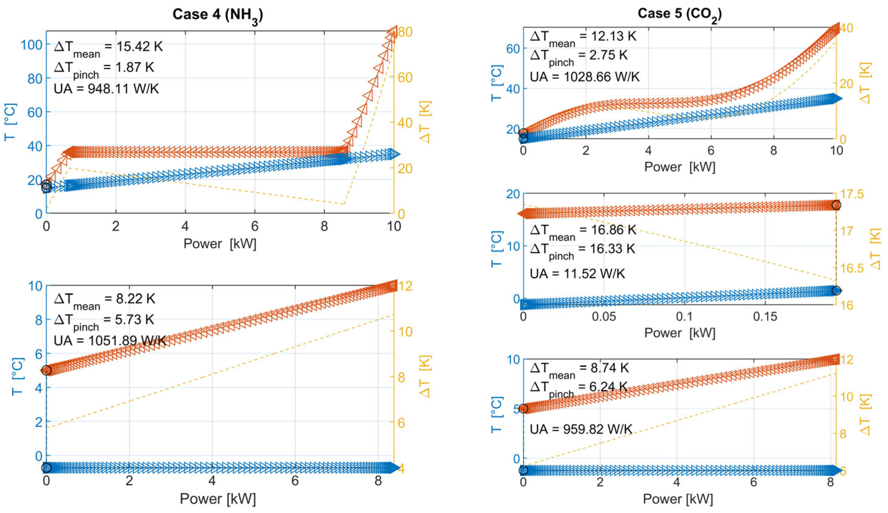
Since the focus here is to identify fast and accurate optimization schemes, and not to find the actual optimized processes, a fixed U -value is used: U = 1000 W/(m2K). However, real HEs will typically operate with significantly different heat transfer coefficients U , depending on parameters such as pressure, if the fluids are liquid or vapor, the type of working fluid and fluid velocities. The optimization algorithm then identifies the best process with a maximum combined HE area A m a x   = 2.0 m2. Figure 2 shows that both condenser and evaporators solutions have approximately 1 m2 heat transfer area. Note that the simplification U = 1000 W/(m2K), made for all HE, transforms the HE area optimizing constraint to a thermal conductance constraint: U A t o t 2000 W/K. Even though this constraint does not relate directly to either cost or HE areas, it is believed that the optimization success to some extent is independent of the heat transfer correlation functions used to model U . That is, if smooth heat transfer correlation functions are used, which are required by high-order integral methods. Hence this problem is viewed as a good starting point for investigating the performance of different optimization schemes.

3. Results and Discussion

All the CO2 processes are transcritical, while all the propane, NH3 and R134a are subcritical processes with condenser pressures significantly less than critical pressure. Figure 2 shows temperature profiles in the heat exchangers for the subcritical heat pump A process with NH3, and the transcritical CO2 process for heat pump B with an internal HE.

3.1. Model Verification

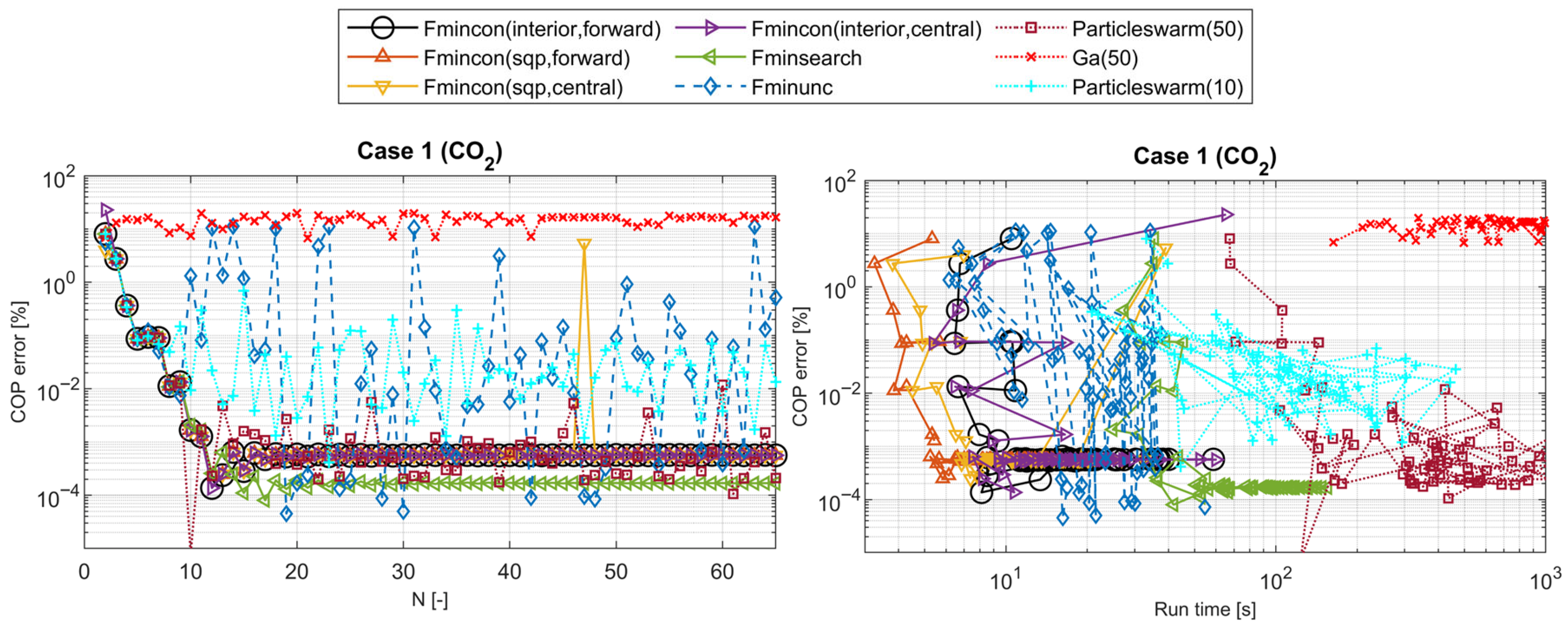
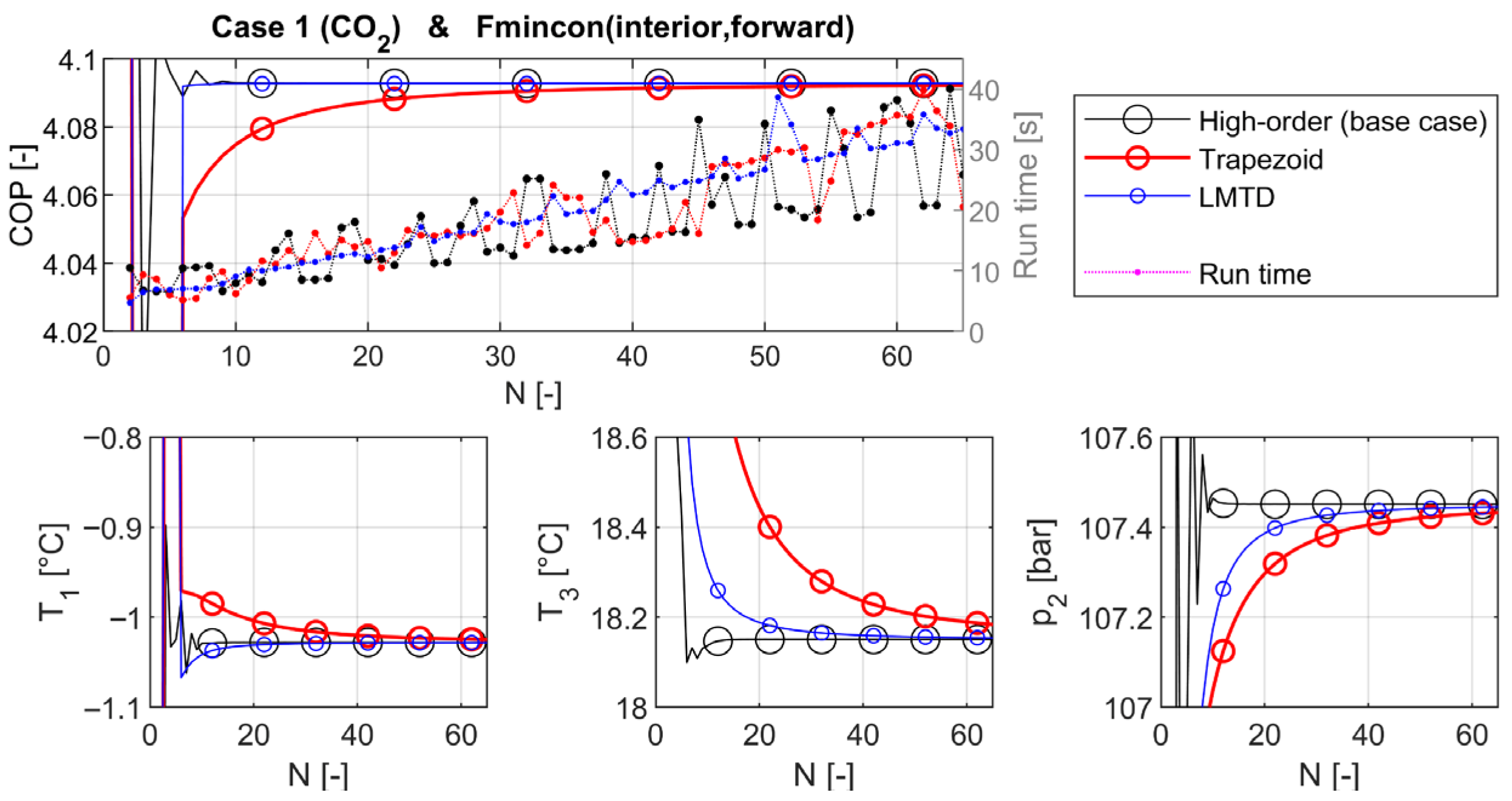
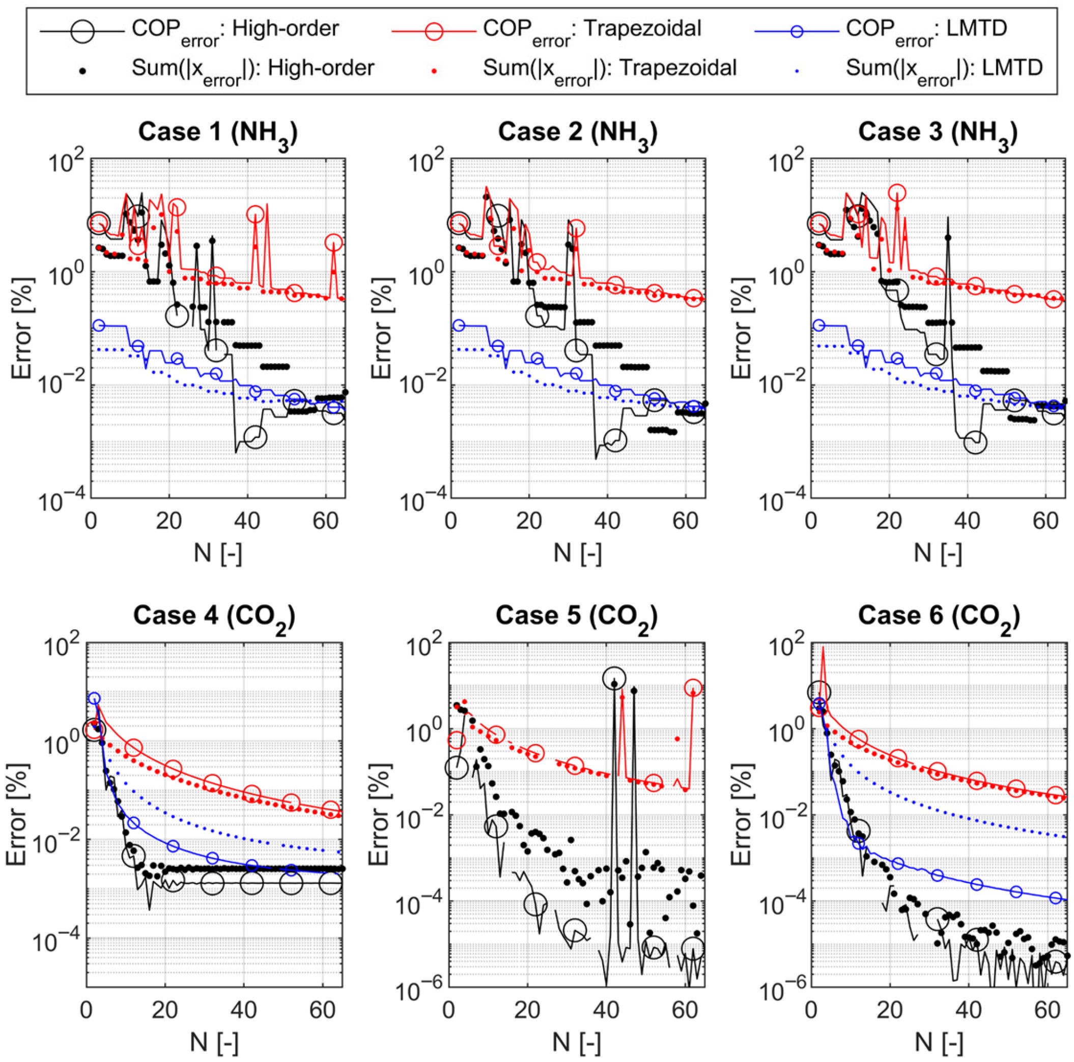
Since an analytical solution is not available, results are validated relative to each other. Figure 3 shows that the best point is detected multiple times with different optimization algorithms, which indicates that the optimal point is identified by the optimization scheme. High-order HE area approximation results are also compared with the conventional LMTD and ‘trapezoidal’ methods in Figure 4, which shows that the different HE models also converge as the number of grid points increases, i.e., obtain the same performance ( C O P o p t i m i z e d ) and optimized variables ( x o p t i m i z e d ). Figure 5 shows that the same is observed for other cases and refrigerants, and that COP errors in high-order and LMTD schemes are typically less than 0.01% for N 40.

3.2. Required Modeling Precision

In this study both 1% and 0.01% optimization accuracy are considered. Modeling COP with a 1% accuracy is often sufficient for the modelling of existing heat pumps because the instrumentation measuring process parameters, such as pressure and temperature, will often have lower precision. However, in optimization studies, which aim to set the optimum starting point for the equipment level design work, it is still important to minimize inaccuracy. For example, the final product is likely to be slightly less efficient if the optimization is terminated early, e.g., when a 1% accuracy is reached, or if numerical approximations are introduced to reduce optimization run time. High accuracy is also required to generate smooth sensitivity plots, which often are essential for understanding trends and design benefits. Figure 4 shows that it is difficult to present sensitivity results based on optimizations with COP error   1%, and that the T 1 , T 3 and p 2 plots are smooth for N   10, i.e., COP error   0.01% is sufficient in a sensitivity study (see Figure 3). Other parameters can be even less sensitive to errors, e.g., even if [4] modelled mixed fluid processes with COP error   0.3 %, the optimized mixtures had component fractions randomly variating between 13–30%.

3.3. Optimization Algorithms

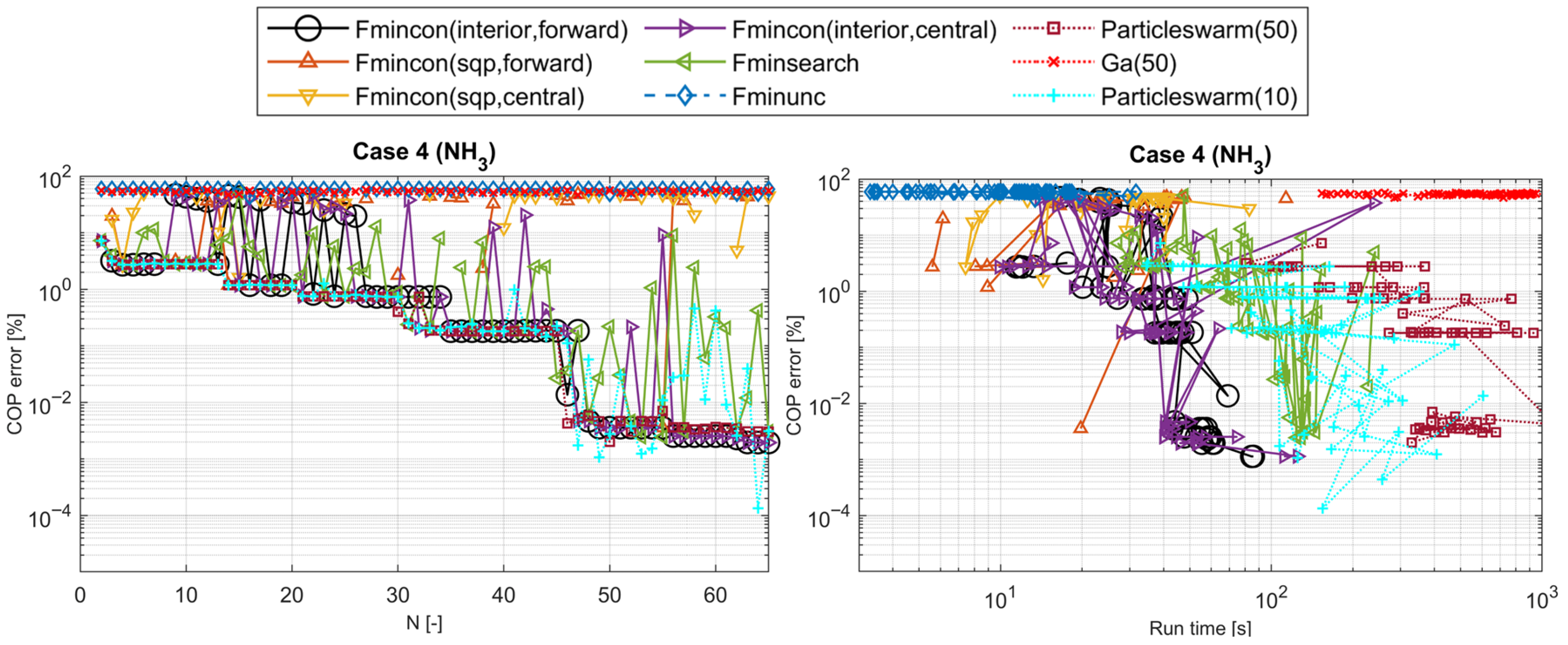
Figure 3 illustrates that Fmincon(sqp,forward) and Fmincon(sqp,cetral) are the fastest algorithms for Case 1 with CO2. However, Figure 6 illustrates that these algorithms frequently fail for Case 4 with NH3, and that Fmincon(interior) is better for obtaining accurate results with COP error less than 1%.
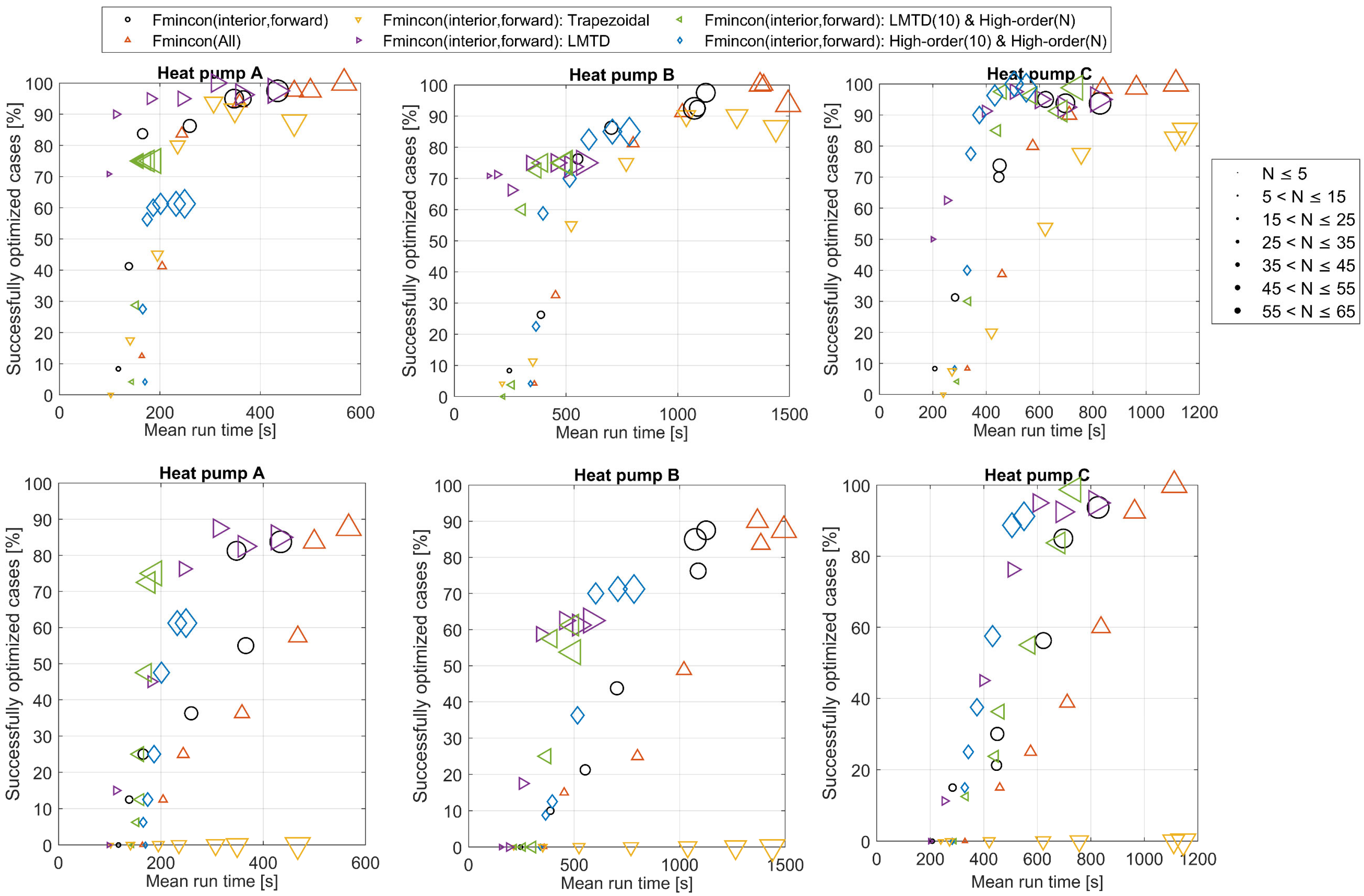
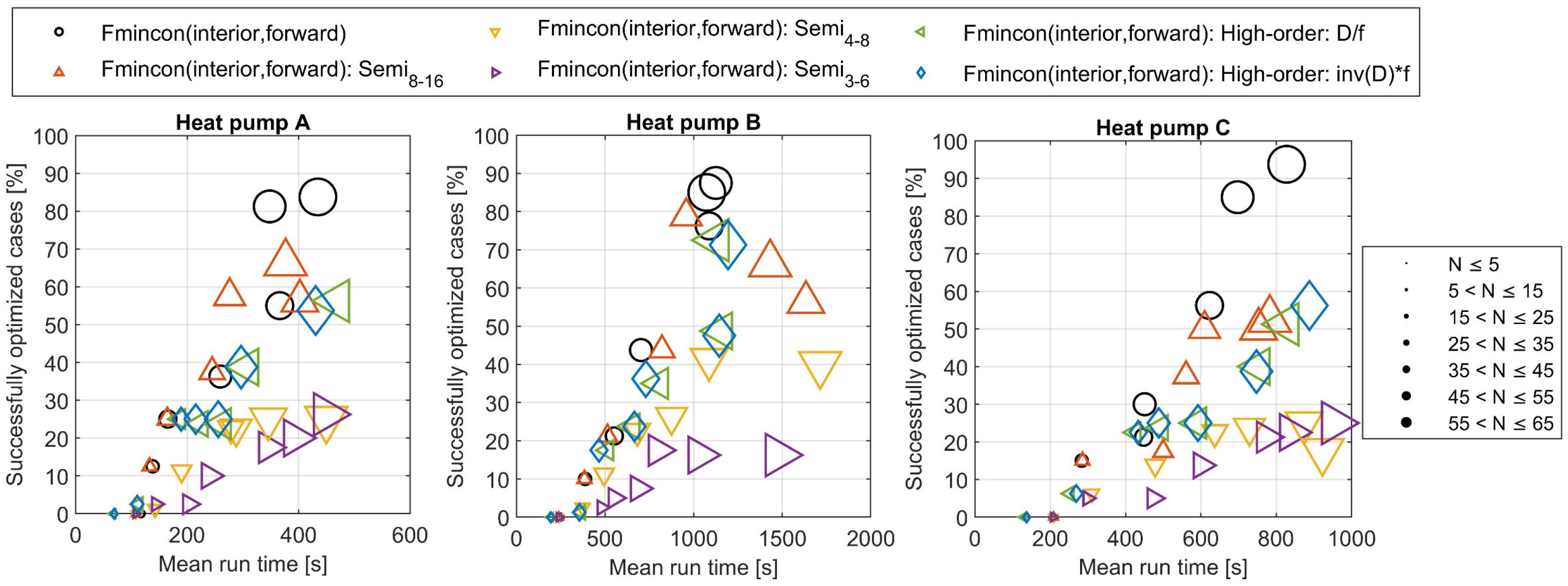
Figure 7 shows a summary of the average optimization success rates and run times. The percentages in Figure 7 are calculated from 80 different optimization results, i.e., each interval is modeled using 10 different grid sizes N , where four different refrigerants and two different cases are modeled for each heat pump design. Figure 7 shows that Fmincon(interior,forward) is overall the most successful optimization algorithm with more than 80% success rate obtaining accurate results with COP error < 0.01% for ‘high-order’ schemes with N 45 grid points. Fmincon(interior,forward) is therefore used later when studying the best HE schemes. Fmincon(interior,cetral) is almost as successful, but is slightly worse for Heat pump B. Fmincon(sqp,forward), Fmincon(sqp,cetral) and Fminsearch are much less accurate than Fmincon(interior,forward), and the Fminsearch optimization is also much more time consuming. All the NH3 optimizations of Case 4 are inaccurate when using Fminunc (see Figure 6), but Figure 3 shows that Fminunc sometimes is successful for Case 1 with CO2. In these successful optimizations, however, Fminunc had about five times larger run time than Fmincon(interior,forward). Particle swarm has a poor success rate for Heat pump C, but PS(50) is often slightly more accurate than Fmincon(interior,forward) for heat pump A and B when producing accurate results with COP error < 0.01%. However, PS(50) is typically 10 times slower, and therefore not recommended. PS(10), with only ten swarm members, is about four times faster than PS(50), but is much less accurate. That is, Fmincon(interior,forward) is both faster and more successful than PS(10). Figure 3 shows that GA is highly inaccurate for Case 1 with CO2, where the initial guess ( x 0 ) generates a system with COP around 1.5. In all cases, GA can improve the design and find processes with COP between 2.5 and 3.1, before the maximum allowed generation span of 300 is exceeded. However, this is far from the optimal COP = 4.0928. The conclusion is that GA is highly inefficient, since the run time after 300 generations is already hundreds of times larger than other more accurate methods. The number of generations required to obtain accurate results is significantly larger, e.g., COP is observed to only increase from 2.738, in generation 200, to 2.756 in the final generation (300). Figure 7 shows that GA has a zero-success rate for all the different designs, as well as being extremely slow. Table 5 summarizes the results and shows that fewer grid points are required to obtain less accurate results with COP error < 1%, i.e., ‘high-order’ schemes requires N 35. However, PS(50) has a 100% success rate heat pump A and B for N 25, which indicates that PS can handle larger HE area errors than Fmincon.

3.4. Sequential Optimization Methods

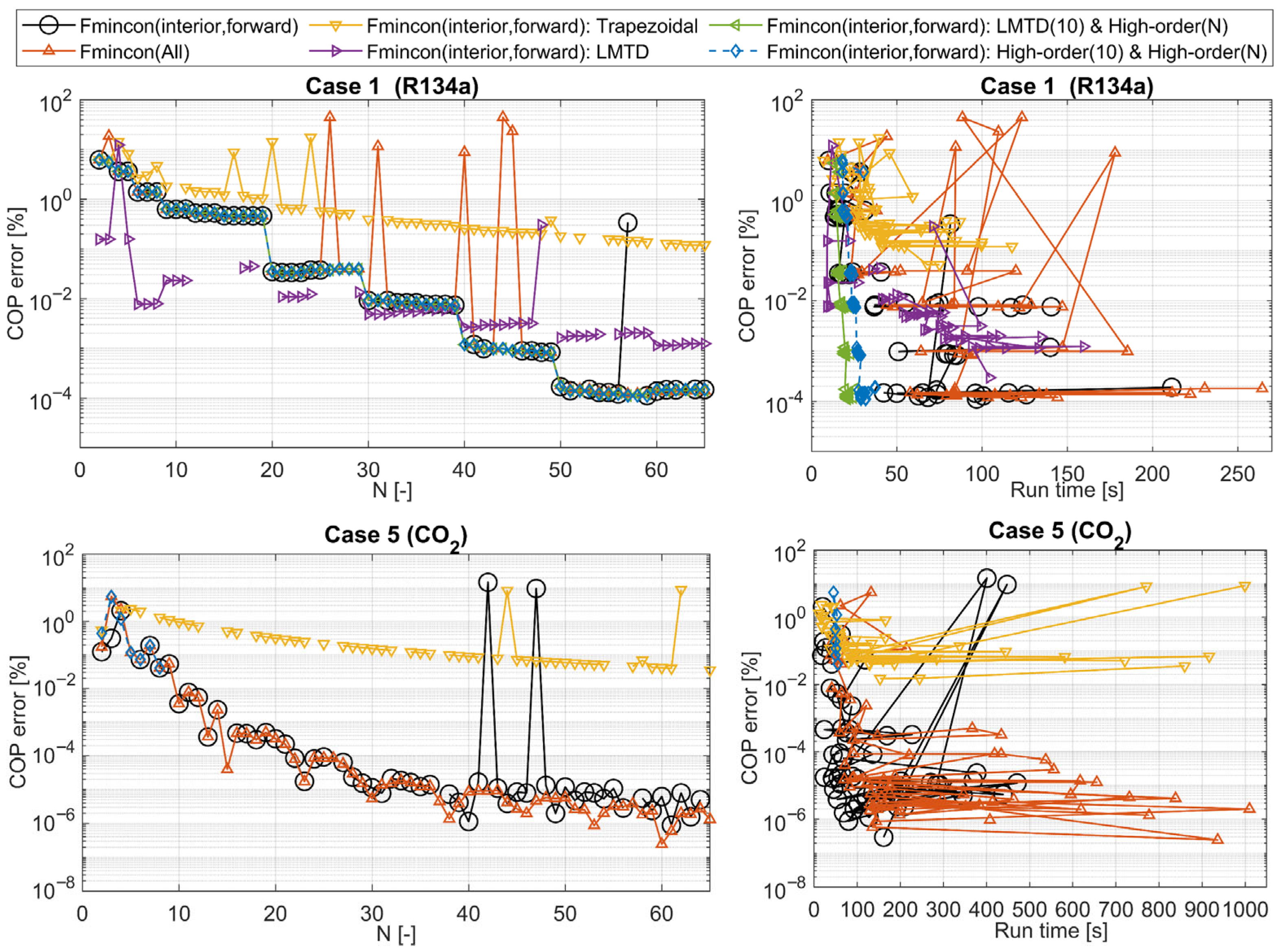
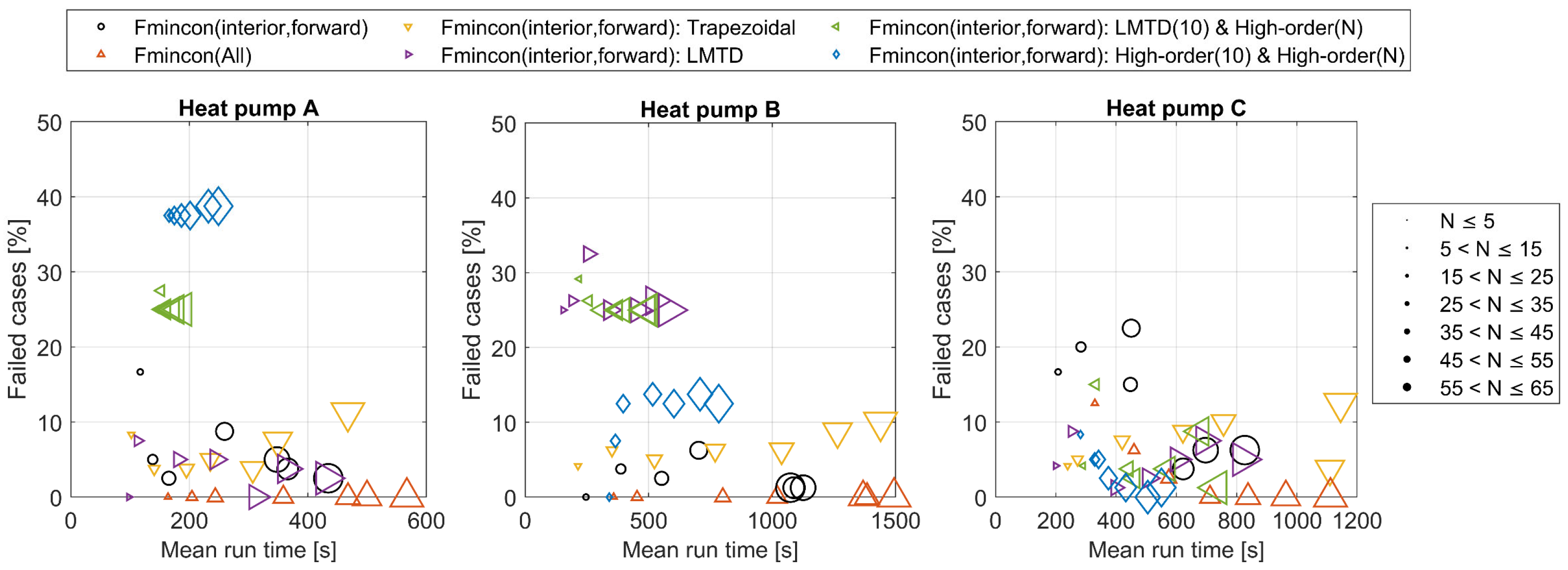
This section explores if the high-order Fmincon(interior,forward) scheme can be further improved using sequential optimization methods, and the results are compared to conventional LMTD and Trapezoidal results. Figure 8 shows a selection of the results to illustrate different performance, Figure 9 gives statistical summary of all the different optimizations, and Figure 10 shows the percentage of optimizations that failed.

3.4.1. Fmincon(All)

Figure 9 shows that Fmincon(interior,forward) results are statistically improved with Fmincon(All). The re-optimizations are often conducted quickly if the initial guess is close to optimal, hence, the three additional optimizations in Fmincon(All) increases run time by less than 30% on average. Figure 8 shows that the Fmincon(interior,forward) sometimes produces inaccurate results and that these results are improved by using Fmincon(All). This scheme calls Fmincon(interior,forward), Fmincon(sqp,forward), Fmincon(interior,central) and Fmincon(sqp,cetral) in a sequence, using the best solution from the previous optimizations as the initial guess. Figure 9 shows that Fmincon(All) improves inaccurate Fmincon(interior,forward) optimizations, and that it is also able to find acceptable solutions were Fmincon(interior,forward) failed. If the first Fmincon(interior,forward) optimization in the Fmincon(All) sequence fails, Fmincon(All) uses a Fmincon(sqp,forward) from the original initial guess. Figure 7 shows that a Fmincon(sqp,forward) method is typical not as accurate as Fmincon(interior,forward), and Figure 8 shows that it is difficult to reoptimize and improve the Fmincon(sqp,forward) results. This is illustrated for Case 1 with R134a in Figure 8, which shows that Fmincon(All) manages to compute find solution when Fmincon(interior,forward) failed, but that some of these values are highly inaccurate (COP error > 50%). Note that Figure 10 shows that Fmincon(All) always managed to a solution. Only the simplest multiple HE systems are studied here, i.e., with two or three HEs. Perhaps even longer Fmincon sequences would be optimal when solving more complex systems. More work is also needed to investigate more complex systems and how default MATLAB values, such as the finite difference step size, can be improved.

3.4.2. Improving the Initial Guess

Optimization run time typically increases with the number of grid points and the number of optimization steps. In this study a rough optimization estimate is generated fast using LMTD and high-order HE schemes with only N = 10 grid points, and by terminating Fmincon(interior,forward) after just 400 function evaluations, instead of the default 3000. These rough estimates are then used as initial guesses for a high-order schemes with N grid points. These optimization sequences are named ‘LMTD(10) & high-order( N )’ and ‘high-order(10) & high-order( N )’, respectively. Figure 9 shows that such sequences require much less run time than Fmincon(interior,forward) for large grids. Heat pump C, with an ejector, is also often optimized with a better success rate, but Heat pump A and B optimizations are less successful due to a larger percentage of failures (see Figure 10). More research is required to identify methods that improvs both run time and success rate.

3.5. Performance of the HE Area Approximations

Different single HE processes were modeled in [2], but this article does not give an accurate picture of how to best model HEs when optimizing multiple HE systems. The aim here is to investigate this, i.e., to compare performance of different optimization schemes based on the analytical LMTD method and other numerical integral approximation of Equation (5), such as high-order, adaptive, trapezoidal, and semi high-order approximations. Note that, a non-constant U -value can be integrated straight forward in the integral expressions defined in Equation (5), which is not the case for the analytical LMTD expression in Equation (8).

3.5.1. High-Order

Of the numerical HE area integral approximation studied here, the high-order method was the most successful with respect to run time. Table 5 shows that schemes with grid size N 35 produce optimal solutions with COP errors 1%, and that N 45 should be used to obtain accurate solutions with COP errors 0.01%, and perhaps even N 55 for heat pump C. A similar optimization study modeling HE with pinch point analysis found that high-order-based schemes with grid size N 10 are sufficient for heat pump A, B and C [27], i.e., in optimization HE area A integral approximations require significantly more grid points than T p i n c h approximations. The results also show that when optimizing systems with multiple HEs, HE area calculations require more grid points than recommended in the non-optimization study of single HE case studies investigated in Ref. [2], where high-order schemes modeled with N 20 were found sufficient for generating HE area A errors 0.01%.

3.5.2. Trapezoidal

Figure 5 and Figure 8 illustrate that large grids are required for low-order trapezoidal schemes to be accurate. Figure 9 shows that at least N 35 should be used to obtain results with COP error 1%, however, the success rate is less than the high-order-based schemes, which are faster since they require fewer grid points. Even trapezoidal schemes with large grids 65 N 55 do not produce any results with COP error less than 0.01%. Results from [2] suggests N 1000 trapezoidal grid points is required to obtain the same accuracy as a N 45 high-order scheme.

3.5.3. High-Order Alternatives

As an alternative to the base case high-order method, the integral is also calculated using the inverse of the high-order differentiation matrix. Figure 11 and Figure 12 show that the ‘high-order: D/f’ and ‘high-order: inv(D)*f’ results are almost identical with respect to optimization success and run time, but they are both less efficient than the high-order method. Figure 12 illustrate that these alternative methods obtain similar results as the high-order method for Case 5 with CO2, while the results are much worse for Case 1 with NH3. Hence, using the high-order differentiation matrix is not recommended. Note that the high-order HE area formula in Equation (12) only computes the whole HE area, and that these alternative methods generates much more accurate results than the trapezoidal for N 35 (e.g., see Figure 9 and Figure 11). Hence, these alternative methods, e.g., with N 65, can still be useful when solving real HE models with pressure drop and heat transfer coefficients, where HE area between grid points must be computed. For example, fluid pressure calculations can require knowledge about the exact position inside the HE, while accurate heat transfer calculations depend on the pressure. The MATLAB matrix backslash operator solves inverse problems using LU factorization or a least squares solver, depending on the condition number of the D matrix. Different methods to solve ill conditioned problems, described by Hansen [44], were tested, however, both truncated singular value decomposition (SVD) and Tikhonov regularization methods made the optimized results worse. Solving inverse problems can be time-consuming for large D matrixes, especially in optimization where inv(D)*f must be computed in each iteration. For high-order schemes with large grids it is therefore possible to compute inv(D) a single time, instead of solving the LU factorization problem in each optimization step. Note that, high-order polynomial integral approximations can also be used to compute HE areas between grid points, but these methods were also found less stable than the high-order method [2]. The optimal approach for solving real HE models needs to be studied further.

3.5.4. Semi High-Order

Figure 11 shows that semi high-order approximations are less accurate, and often require more run time. Figure 12 shows that for a given grid size N , the semi high-order approximations with 3–6 grid points in each element (Semi3–6) is more accurate than trapezoidal, and the accuracy is improved by increasing the order, i.e., reducing the number of elements and increasing the number of nodes in each element. However, the semi high-order approximations are less accurate than the high-order method. Also, a semi high-order method based on the high-order differentiation matrix is even less successful when reducing the order of the integral approximation (see ‘Semi4–8: D/f’ in Figure 12).

3.5.5. Adaptive Methods

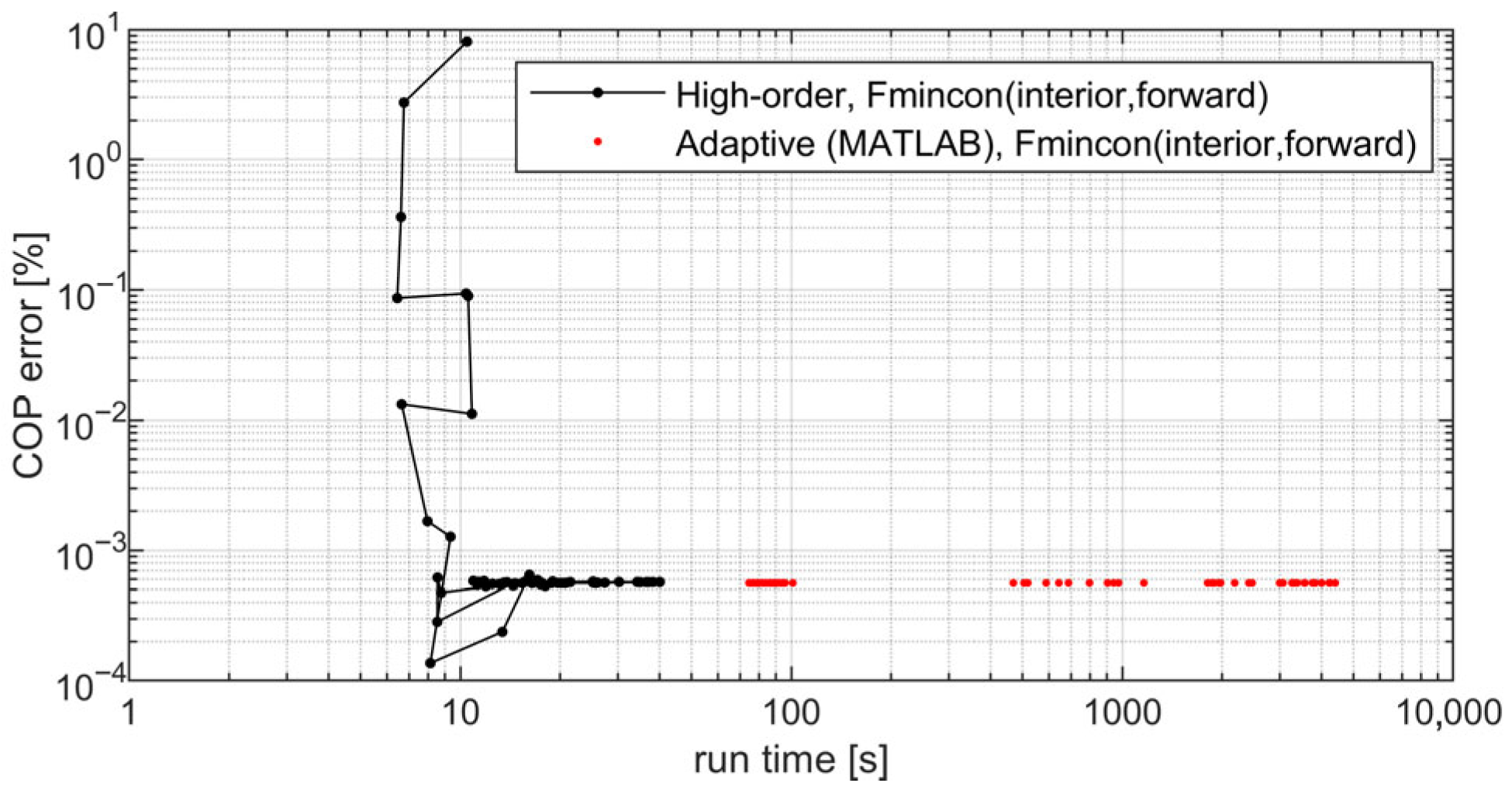
This method has been applied by Chen [21]. MATLAB includes an adaptive integral named ‘integral’. Such functions are designed to be very robust since they are designed to solve all forms of integrals. The ‘integral’ function divides the problem into 10 sections with 15 grid points each. The adaptive ‘integral’ function in MATLAB is terminated if the number of sections become larger than 16,384. It then identifies sections which may include inaccuracies, and divides them into smaller sections. This approach turned out to be very inefficient, and Figure 13 shows that it is 9–500 times slower than the high-order method with N 10. Figure 13 includes many optimization results where the ‘integral’ function returned a warning that the maximum limit of 16,384 sections has been reached, i.e., computing N > 200 000 grid points. Calculating that many grid points requires a lot of run time, and optimizations where this warning occurred, i.e., one or multiple times, were highly inefficient with run times around 450–4500 s. Optimizations without warnings were much faster with run times around 100 s. Note that, Figure 13 shows that the adaptive method produces results with similar accuracy as the much faster high-order method with N 10. That is, the large initial N = 150 grid points used by ‘integral’ is not ideal for the HE problems studied here and should probably be reduced, e.g., by only using one initial section. However, the main finding in Figure 13 is that the adaptive ‘integral’ function in MATLAB is inefficient and should therefore not be used. Adaptive algorithms are not designed for solving HE, since such problems can be non-smooth if the fluid property package struggles to compute one internal grid point accuracy [2]. This is especially true in optimization studies since they can require the solution of thousands of different integrals. Adaptive methods require high computational resources for calculating integrals that cannot be solved accurately, which is due to numerical noise generated by inaccuracies in the fluid property packages. A fixed approach, such as the high-order method, calculates non-smooth HE problems with less accuracy, but quickly moves on to the next optimization step where the integral often can be computed accurately. Since the adaptive method is inefficient, this article will focus on finding fast accurate schemes with a fixed approach that are able to calculate special non-smooth problems with sufficient precision to ensure high optimization success rate.

3.5.6. LMTD

The LMTD method derived in Equation (8) is an approximation, which assumes that the average U -value is known between all the neighboring node points, i.e., U ¯ i j U i j + U i j 1 / 2 . However, this is a first-order approximation, which can be highly inaccurate, perhaps similar to the low-order Trapezoidal method (see Figure 9). In this study, the LMTD method might appear more successful than it actually is since the U -value is assumed to be constant U i j = U i j 1 = 1000 W/(m2K), which make the first-order approximation exact: U ¯ i j = 1000 W/(m2K). It can be problematic to expand the LMTD model with real heat HE models, where U i j is changing and is computed accurately at each grid point. More research is vital to determine the performance of LMTD methods in such cases.
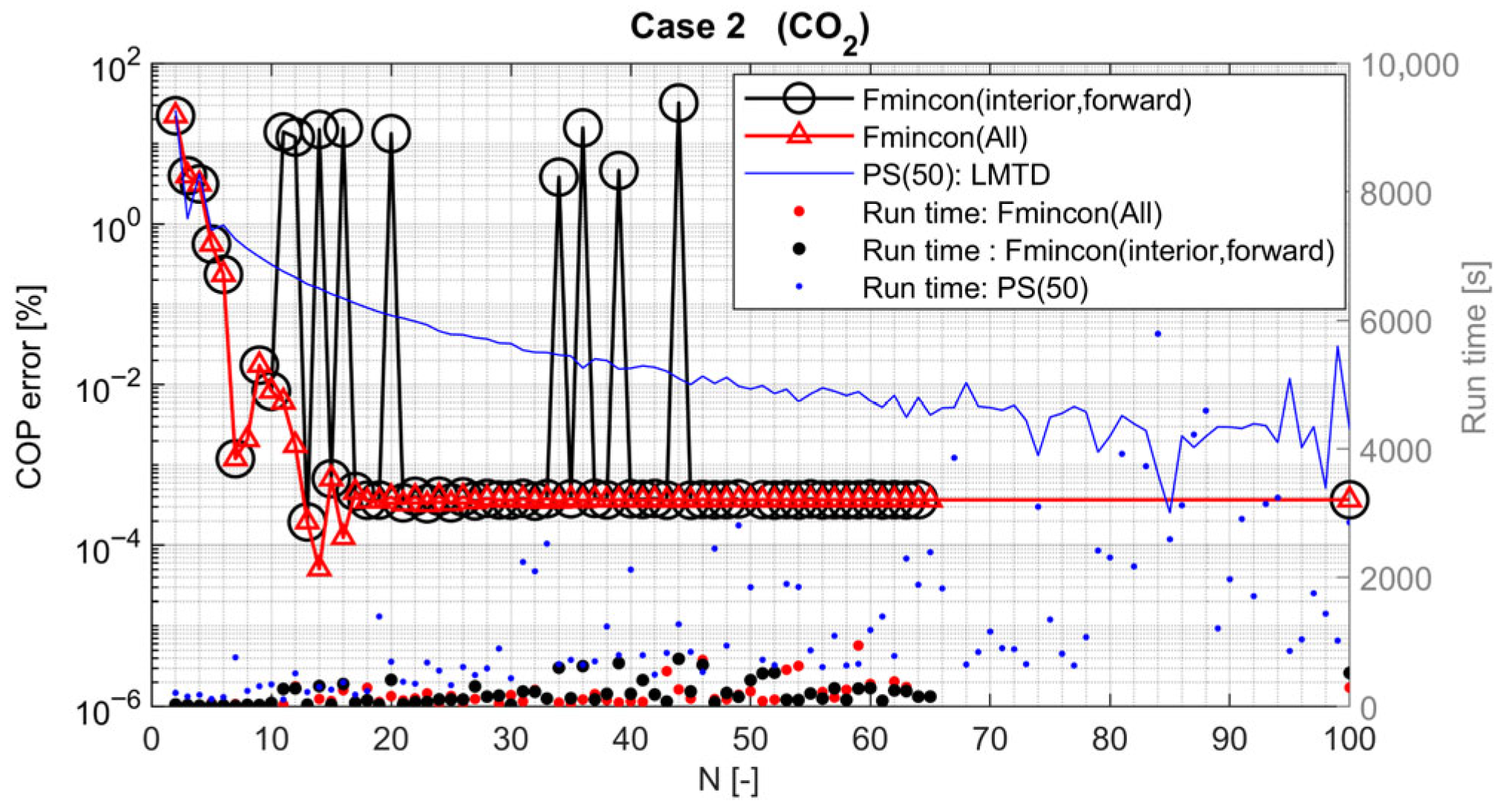
When assuming constant U-values, Figure 9 shows that there is not much to gain by increasing the number of nodes beyond N 25 in the LMTD schemes. Figure 9 also shows that a small grids, N 5, generates results where more than 50% of the solutions have COP error less than 1%. For the subcritical processes modeled, the LMTD method is typically better than high-order. Figure 5 shows that both the optimization variables ( x ) and COP are modeled accurately with the LMTD method for Case 1, 2 and 3 with NH3, i.e., all having errors less than 0.1% for N   5. Figure 8 shows that this is also true if modeling the subcritical R134a, where the high-order method only produces more accurate results than the LMTD method if N 40. However, the LMTD method assumes that the heat capacity is constant, which is a highly inaccurate assumption for the transcritical CO2 processes. For example, Chen have concluded that CO2 gas coolers could be 30–60% undersized with LMTD methods based on HE inlet and outlet values, i.e., schemes with N = 2 [21]. Ref. [2] identified transcritical CO2 processes were LMTD schemes were even less accurate than trapezoidal for a given grid size, and that LMTD schemes with N 1000 grid points produced results with less accuracy than a high-order scheme with N   45. The transcritical processes modeled here with LMTD, however, require far fewer grid points. Figure 5 shows that the LMTD method it better at finding an accurate optimized COP value than finding optimal optimization parameters in the transcritical CO2 processes. That is, while the COP and x errors typically are about the same size in high-order and trapezoidal schemes (see Figure 5), the x error is typically much larger in the LMTD schemes, e.g., Figure 5 illustrates that more than N 40 grid points are required to obtain s u m ( x e r r o r )   0.01%. That is, the LMTD method is likely to overestimate one HE and underestimating another, which to some extent cancels each other out when modeling the COP for the whole process. However, this cancelling is not perfect and Figure 5 also shows that the LMTD method requires about twice as many grid points as the high-order method for Case 4 with CO2 to obtain COP errors 0.01%. In addition, the LMTD optimizations of the CO2 heat pump B (Case 2 and 5) always fails for the nonlinear constrained gradient-based method Fmincon(interior,forward). However, a particleswarm scheme can be used to optimize Case 2 with CO2, as illustrated in Figure 14, which shows that N 50 are required to obtain similar results as a high-order Fmincon(interior,forward) scheme with N 10. This scheme is very inefficient and typically requires 2000% more run time than a high-order Fmincon(interior,forward) scheme.

3.5.7. Possible Applications and Real Heat Transfer Models

This study only investigates constant U -value cases, but it is believed that the novel high-order method also offers similar advantage for solving HE integrals with non-constant U -value. That is, if the heat transfer models are designed to generate a continuous and smooth U function, such as in [23]. However, high-order integration methods are inaccurate if heat transfer functions are based on non-smooth step functions, which have been suggested to model different flow regimes, see [18,45].
The high-order HE area approximation can also be used to develop accurate heat transfer models from experimental HE data, instead of using conventional LMTD and trapezoidal schemes. For example, Longo et al. used a relatively accurate HE area integral approximation based on a trapezoid method using 100 grid points (see Figure 5), and reported only a 4.7% mean absolute percentage deviation between modeled and experimental data for condensation in brazed plate HEs [18]. Amalfi et al. reported that the best flow boiling heat transfer models obtained a mean absolute errors of 22.1% [14]. The accuracy of the HE area approximation can be a significant factor for the size of such errors, however, the number of grid points used to derive the heat transfer models is sometimes not even mentioned in articles. For example, Figure 14 shows that N = 2 schemes are highly inaccurate, generating COP error > 20%.

4. Conclusions

The results show that the optimization of even relatively simple problems with only two or three HEs can be very time-consuming if an inefficient optimization scheme is used, e.g., a single optimization can require more than an hour while the best schemes use less than 10 s. Note that optimization of real heat pumps will be much more time consuming since realistic heat transfer models require additional internal HE values, such as specific heat, mass density and viscosity. It is also assumed that a fixed retailer HE design is used, since optimization run-time will increase if the HE design is optimized. However, HE area integral approximations are central in all optimization schemes, and the main finding of this study is that high-order HE area approximation schemes with integral weights offer significant advantages when optimizing systems with multiple HEs, i.e., better success rate for a given run time. At least N 35 should be used to obtain results with COP error 1%, and at least N 45 to obtain results with COP error 0.01 %. Accurate solutions of high-order schemes can be obtained much faster than with conventional low-order integral methods, such as trapezoid. Adaptive methods available in math-programing software to solve general integrals, such as the ‘integral’ function in MATLAB, can be extremely time consuming when optimizing HE systems. Fast LMTD approximation methods, with only few grid points N 5, can be very successful for subcritical heat pump processes operating far from the critical point, e.g., Case 1, 2 and 3 with NH3. However, one must be careful using LMTD schemes with few grid points, since some processes require larger grids. Since the LMTD method cannot be directly expanded to problems with non-constant U -values, this study recommends high-order methods when modeling real HE processes based on accurate heat transfer models. However, more work is needed to study HE with non-constant U -values.
In the study of different optimization methods, the results show that nonlinear constrained gradient-based methods, such as Fmincon, are best suited for the heat pump optimization cases studies here. The interior method is more successful than sqp, and the interior method is also slightly better if gradients are computed with forward difference methods, instead of central difference. Fmincon(interior,forward) is about 10 times faster than PS(50), which is the best stochastic method identified. GA is perhaps the most conventional method [36], and has similar run time as PS(50), but it is typically not able to generate accurate results and should therefore not be used. The Fmincon optimalization method can be further improved by using the optimization sequence Fmincon(All), and in some cases this achieves a 100% success rate. Perhaps even longer optimization sequences, than the four used in Fmincon(All), should be used when solving more complex systems with more the three HEs. Run time can be reduced significantly by using a faster method with less grid points to improve the initial guess, and for heat pump C with an ejector the success rate even improved. However, although the idea of using inaccurate optimization schemes to quickly find a first approximation seems promising, more research is required to identify methods that are both successful and faster than a single optimization. Although the case studies in the present work are limited to three different heat pump designs and constant U -values, it is believed the findings provide several general insights into the optimization of other process systems and smooth non-cons tant U -value functions.
Further work should explore the real-world benefits of the recommended optimization schemes, i.e., also include realistic cost and heat transfer models for all the different HEs in the heat pump (evaporator, gas cooler, condenser and internal HE). If accurate heat transfer and cost models are applied, such schemes should be able to identify optimal sets of HEs with respect to cost. The ultimate real-world validation of such optimization schemes is perhaps an experiment investigating an already existing heat pump, where the HEs are designed and sized according to the best conventional methods used by industry. An optimization will then reveal if it is possible to design a more energy efficient heat pump without increasing cost. The optimized results can also be tested and validated through experiments if the heat pump is modified, i.e., replacing the old HEs with a new optimized set that has the same combined cost, but sized and designed better.

Funding

This research received no external funding.

Data Availability Statement

The relevant data are presented within the article.

Conflicts of Interest

The author declares no conflicts of interest.

References

  1. Allen, B.; Savard-Goguen, M.; Gosselin, L. Optimizing heat exchanger networks with genetic algorithms for designing each heat exchanger including condensers. Appl. Therm. Eng. 2009, 29, 3437–3444. [Google Scholar] [CrossRef]
  2. Amalfi, R.L.; Vakili-Farahani, F.; Thome, J.R. Flow boiling and frictional pressure gradients in plate heat exchangers. Part 2: Comparison of literature methods to database and new prediction methods. Int. J. Refrig. 2016, 61, 185–203. [Google Scholar] [CrossRef]
  3. Austbø, B.; Løvseth, S.W.; Gundersen, T. Annotated bibliography—Use of optimization in LNG process design and operation. Comput. Chem. Eng. 2014, 71, 391–414. [Google Scholar] [CrossRef]
  4. Ayub, Z.H. Plate Heat Exchanger Literature Survey and New Heat Transfer and Pressure Drop Correlations for Refrigerant Evaporators. Heat Transf. Eng. 2003, 24, 3–16. [Google Scholar] [CrossRef]
  5. Ayub, Z.H.; Khan, T.S.; Salam, S.; Nawazc, K.; Ayub, A.H.; Khan, M.S. Literature survey and a universal evaporation correlation for plate type heat exchangers. Int. J. Refrig. 2019, 99, 408–418. [Google Scholar] [CrossRef]
  6. Bell, I.H.; Wronski, J.; Quoilin, S.; Lemort, V. Pure and Pseudo-pure Fluid Thermophysical Property Evaluation and the Open-Source Thermophysical Property Library CoolProp. Ind. Eng. Chem. Res. 2014, 53, 2498–2508. [Google Scholar] [CrossRef]
  7. Brodal, E.; Eiksund, O. Optimization study of heat pumps using refrigerant blends—Ejector versus expansion valve systems. Int. J. Refrig. 2020, 111, 136–146. [Google Scholar] [CrossRef]
  8. Brodal, E.; Jackson, S.; Eiksund, O. Performance and design study of optimized LNG Mixed Fluid Cascade processes. Energy 2019, 189, 116207. [Google Scholar] [CrossRef]
  9. Brodal, E.; Jackson, S.; Eiksund, O. Comparing optimization schemes for solving case studies with multiple heat exchangers using high-order pinch point temperature difference methods. Comput. Chem. Eng. 2023, 180, 108474. [Google Scholar] [CrossRef]
  10. Brodal, E.; Jackson, S.; Hailu, G. UA and pinch point temperature difference modeling—Finding the best heat exchanger schemes. Comput. Chem. Eng. 2022, 169, 108085. [Google Scholar] [CrossRef]
  11. Byrd, R.H.; Hribar, M.E.; Nocedal, J. An interior point algorithm for large-scale nonlinear programming. SIAM J. Optim. 1999, 9, 877–900. [Google Scholar] [CrossRef]
  12. Chen, Y.-G. Pinch point analysis and design considerations of CO2 gas cooler for heat pump water heaters. Int. J. Refrig. 2016, 69, 136–146. [Google Scholar] [CrossRef]
  13. Dai, B.; Dang, C.; Li, M.; Tian, H.; Ma, Y. Thermodynamic performance assessment of carbon dioxide blends with low-global warming potential (GWP) working fluids for a heat pump water heater. Int. J. Refrig. 2015, 56, 1–14. [Google Scholar] [CrossRef]
  14. Dimian, A.C.; Bildea, C.S.; Kiss, A.A. Chapter 13—Pinch Point Analysis. Comput. Aided Chem. Eng. 2014, 35, 525–564. [Google Scholar]
  15. Duran, M.A.; Grossmann, I.E. Simultaneous optimization and heat integration of chemical processes. AIChE J. 1986, 32, 123–138. [Google Scholar] [CrossRef]
  16. Elbel, S.; Hrnjak, P. Experimental validation of a prototype ejector designed to reduce throttling losses encountered in transcritical R744 system operation. Int. J. Refrig. 2008, 31, 411–422. [Google Scholar] [CrossRef]
  17. Eldeeb, R.; Aute, V.; Radermacher, R. A survey of correlations for heat transfer and pressure drop for evaporation and condensation in plate heat exchangers. Int. J. Refrig. 2016, 65, 12–26. [Google Scholar] [CrossRef]
  18. Elias, A.M.; Giordano, R.d.C.; Secchi, A.R.; Furlan, F.F. Integrating pinch analysis and process simulation within equa-tion-oriented simulators. Comput. Chem. Eng. 2019, 130, 106555. [Google Scholar] [CrossRef]
  19. Fu, C.; Gundersen, T. Heat and work integration: Fundamental insights and applications to carbon dioxide capture processes. Energy Convers. Manag. 2016, 121, 36–48. [Google Scholar] [CrossRef]
  20. Gao, K.; Wu, J.; Bell, I.; Lemmon, E. Thermodynamic properties of ammonia for temperatures from the melting line to 725 K and pressures to 1000 MPa. J. Phys. Chem. Ref. Data 2020. [Google Scholar]
  21. Hansen, P.C. Discrete Inverse Problems: Insight and Algorithms; Society for Industrial and Applied Mathematics: Philadelphia, PA, USA, 2010. [Google Scholar]
  22. Hesthaven, J.S.; Gottlieb, S.; Gottlieb, D. Spectral Methods for Time-Dependent Problems; Cambridge University Press: Cambridge, UK, 2007. [Google Scholar]
  23. Kemp, I.C. Preface. In Pinch Analysis and Process Integration, 2nd ed.; Butter-worth-Heinemann: Oxford, UK, 2007; pp. xiv–xv. [Google Scholar]
  24. Kennedy, J.; Eberhart, R. Particle swarm optimization. In Proceedings of the ICNN’95—International Conference on Neural Networks, Perth, Australia, 27 November–1 December 1995. [Google Scholar]
  25. Kim, S.Y.; Bagajewicz, M. Global optimization of heat exchanger networks using a new generalized superstruc-ture. Chem. Eng. Sci. 2016, 147, 30–46. [Google Scholar] [CrossRef]
  26. Kim, Y.; Lim, J.; Shim, J.Y.; Hong, S.; Lee, H.; Cho, H. Optimization of Heat Exchanger Network via Pinch Analysis in Heat Pump-Assisted Textile Industry Wastewater Heat Recovery System. Energies 2022, 15, 3090. [Google Scholar] [CrossRef]
  27. Kruzel, M.; Bohdal, T.; Dutkowski, K.; Wołosz, K.J.; Robakowski, G. The Heat Transfer Coefficient During Pool Boiling of Refrigerants in a Compact Heat Exchanger. Energies 2025, 18, 4030. [Google Scholar] [CrossRef]
  28. Lemmon, E.W.; McLinden, M.O.; Wagner, W. Thermodynamic Properties of Propane. III. A Reference Equation of State for Temperatures from the Melting Line to 650 K and Pressures up to 1000 MPa. J. Chem. Eng. Data 2009, 54, 3141–3180. [Google Scholar] [CrossRef]
  29. Levy, S. Genetic Algorithms in Search Optimization and Machine Learning; New Whole Earth LLC: Chicago, IL, USA, 1991; 126p. [Google Scholar]
  30. Longo, G.A.; Righetti, G.; Zilio, C. A new computational procedure for refrigerant condensation inside herringbone-type Brazed Plate Heat Exchangers. Int. J. Heat Mass Transf. 2015, 82, 530–536. [Google Scholar] [CrossRef]
  31. Matlab. 9.8.0.1323502 (R2020a), The MathWorks Inc.: Natick, MS, USA, 2020.
  32. Nelder, J.A.; Mead, R. A Simplex Method for Function Minimization. Comput. J. 1965, 7, 308–313. [Google Scholar] [CrossRef]
  33. Powell, M.J.D. A Fast Algorithm for Nonlinearly Constrained Optimization Calculations; Springer: Berlin/Heidelberg, Germany, 2006; pp. 144–157. [Google Scholar]
  34. Rao, R.V.; Saroj, A.; Ocloń, P.; Taler, J. Design Optimization of Heat Exchangers with Advanced Optimization Techniques: A Review. Arch. Comput. Methods Eng. 2019, 27, 517–548. [Google Scholar] [CrossRef]
  35. Ren, C.; Song, Q.; Sun, S.; Zhang, C.; Wang, D. Experimental Study on Flow Boiling Heat Transfer of Zeotropic Mixture R290/R601a in a Mini-Channel. Energies 2025, 18, 2074. [Google Scholar] [CrossRef]
  36. Shampine, L. Vectorized adaptive quadrature in MATLAB. J. Comput. Appl. Math. 2008, 211, 131–140. [Google Scholar] [CrossRef]
  37. Shanno, D.F. Conditioning of Quasi-Newton Methods for Function Minimization. Math. Comput. 1970, 24, 647–656. [Google Scholar] [CrossRef]
  38. Span, R.; Wagner, W. A New Equation of State for Carbon Dioxide Covering the Fluid Region from the Triple-Point Temperature to 1100 K at Pressures up to 800 MPa. J. Phys. Chem. Ref. Data 1996, 25, 1509–1596. [Google Scholar] [CrossRef]
  39. Spellucci, P. A new technique for inconsistent QP problems in the SQP method. Math. Methods Oper. Res. 1998, 47, 355–400. [Google Scholar] [CrossRef]
  40. Szymczak, P.; Jasiński, P.B.; Łęcki, M. Numerical Study of the Condenser of a Small CO2 Refrigeration Unit Operating Under Supercritical Conditions. Energies 2025, 18, 2992. [Google Scholar] [CrossRef]
  41. Tillner-Roth, R.; Baehr, H.D. An International Standard Formulation for the Thermodynamic Properties of 1,1,1,2-Tetrafluoroethane (HFC-134a) for Temperatures from 170 K to 455 K and Pressures up to 70 MPa. J. Phys. Chem. Ref. Data 1994, 23, 657–729. [Google Scholar] [CrossRef]
  42. Trefethen, L.N. Spectral Methods in Matlab; SIAM: Philadelphia, PA, USA, 2000. [Google Scholar]
  43. Vikse, M.; Watson, H.A.; Kim, D.; Barton, P.I.; Gundersen, T. Optimization of a dual mixed refrigerant process using a nonsmooth approach. Energy 2020, 196, 116999. [Google Scholar] [CrossRef]
  44. Kumar, D.V.; Vijayaraghavan, S.; Thakur, P. Analytical and experimental investigation on heat transfer and flow parameters of Multichannel louvered fin cross flow heat exchanger using iterative LMTD and ∊-NTU method. Mater. Today Proc. 2022, 52, 1240–1248. [Google Scholar] [CrossRef]
  45. Watson, H.A.J.; Khan, K.A.; Barton, P.I. Multistream heat exchanger modeling and design. AIChE J. 2015, 61, 3390–3403. [Google Scholar] [CrossRef]
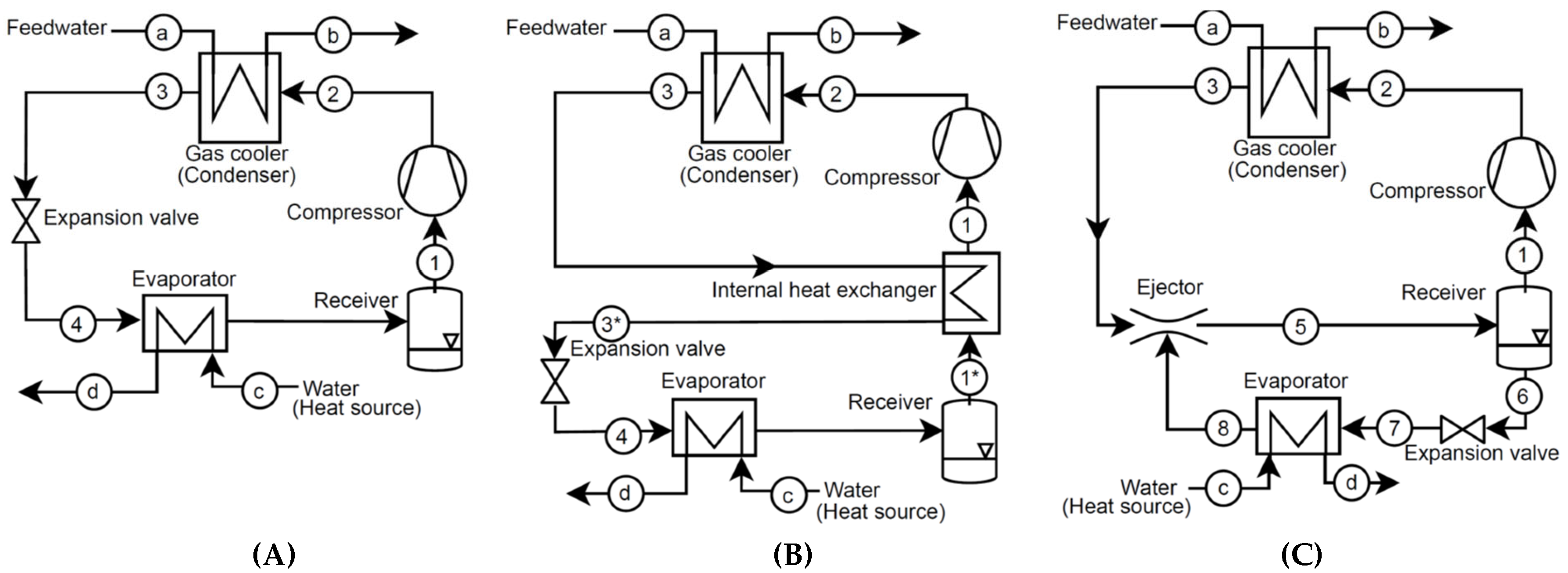
Figure 1. Heat pump (AC). Figure is adapted from Ref. [9].
Energies 18 05270 g001
Figure 2. Optimized temperature profiles in the HEs. Case 4 with NH3 (left) and Case 5 with CO2 (right).
Energies 18 05270 g002
Figure 3. Optimization errors for different optimization algorithms using ‘high-order’ grid points with respect to grid size N (left) and computer run time (right).
Energies 18 05270 g003
Figure 4. Fmincon (interior,forward) optimized results for Case 1 with CO2 using different HE area approximations (High-order, Trapezoidal and LMTD) and number of grid points ( N ).
Energies 18 05270 g004
Figure 5. Fmincon(interior,forward) optimization errors for different cases and HE area approximations. Points missing indicates that the optimization failed, e.g., all LMTD-based optimization of Case 5 failed.
Energies 18 05270 g005
Figure 6. Errors in optimized COP using the ‘high-order’ method versus grid size N (left) and run time (right).
Energies 18 05270 g006
Figure 7. Percentage of successfully optimized problems, using the ‘high-order’ HE method, as a function of mean run time. Top: COP error < 1%. Bottom: COP error < 0.01%.
Energies 18 05270 g007
Figure 8. Optimized errors for different working fluids and optimization schemes.
Energies 18 05270 g008
Figure 9. Percentage of successfully optimized problems as a function of mean run time. Top: error COP < 1%. Bottom: COP error < 0.01%.
Energies 18 05270 g009
Figure 10. Percentage of optimizations that failed, i.e., violating the default MATLAB optimization tolerances or the user defined constraint tolerance: a b s ( A t o t A m a x )   > 0.001 m2.
Energies 18 05270 g010
Figure 11. Percentage of successfully optimized problems with COP error < 0.01%.
Energies 18 05270 g011
Figure 12. Optimized errors for different integral approximations using Fmincon(interior,forward).
Energies 18 05270 g012
Figure 13. Optimized errors versus run time for Case 1 with CO2.
Energies 18 05270 g013
Figure 14. Optimized errors and run time for Case 2 with CO2.
Energies 18 05270 g014
Table 1. Optimization variables x , initial vales x 0 , and lower LB and upper UB bounds.
x :
Heat Pump A
x :
Heat Pump B
x :
Heat Pump C
Initial Guess
x 0
LBUB
T1T1T8273.15 K (1 − 0.01 (0.5 − rand))0 K500 K
T3T3T3223.15 K (1 − 0.01 (0.5 − rand))0 K500 K
p2p2p295 bar (1 − 0.01 (0.5 − rand))1 bar1000 bar
-T1*-15 °C (1 − 0.01 (0.5 − rand))1 × 10⁻⁶ °C100 °C
--pr4 (1 − 0.01 (0.5 − rand))145
Table 4. Definition of cases, which are optimized for different refrigerants (R).
Case 1 (R)Case 2 (R)Case 3 (R)Case 4 (R)Case 5 (R)Case 6 (R)
Heat pumpABCABC
T b 70 °C70 °C70 °C35 °C35 °C35 °C
Table 2. Input parameters.
Heat PumpInputs Process SchemeInputs Optimization Scheme
A R , P g a s   c o o l e r , T a , T b , T c , T d , T 1 , T 3 , p 2 and η c o m p A m a x and x 0
B R , P g a s   c o o l e r , T a , T b , T c , T d , T 1 , T 3 , T 1 * , p 2 and η c o m p A m a x and x 0
C R , P g a s   c o o l e r , T a , T b , T c , T d , T 8 , T 3 , p 2 , p r   a n d   η c o m p A m a x , η e j e c t o r   and x 0
Table 3. Output parameters.
Heat PumpOutputs Process SchemeOutputs Optimization Scheme
A Δ T p i n c h   e v a p o r a t o r , Δ T p i n c h   g a s   c o o l e r , A t o t and COP C O P o p t i m i z e d and x o p t i m i z e d
B Δ T p i n c h   e v a p o r a t o r , Δ T p i n c h   g a s   c o o l e r , Δ T p i n c h   I H E , A t o t and COP C O P o p t i m i z e d and x o p t i m i z e d
C Δ T p i n c h   e v a p o r a t o r , Δ T p i n c h   g a s   c o o l e r , A t o t , η m o d e l l e d   e j e c t o r and COP C O P o p t i m i z e d and x o p t i m i z e d
Table 5. Recommended schemes using the ‘high-order’ HE model.
Heat PumpCOP Error Less ThanBest Optimization Scheme
Optimization AlgorithmGrid Size
A1.00%Fmincon(interior) 35 < N
B1.00%Fmincon(interior,forward) 35 < N
C1.00%Fmincon(interior,forward) 35 < N
A0.01%Fmincon(interior) 45 < N
B0.01%Fmincon(interior,forward) 45 < N
C0.01%Fmincon(interior) 55 < N
Disclaimer/Publisher’s Note: The statements, opinions and data contained in all publications are solely those of the individual author(s) and contributor(s) and not of MDPI and/or the editor(s). MDPI and/or the editor(s) disclaim responsibility for any injury to people or property resulting from any ideas, methods, instructions or products referred to in the content.