A Physics-Informed Variational Autoencoder for Modeling Power Plant Thermal Systems

Abstract

Data-driven models for complex thermal systems face two main challenges: a heavy dependence on high-quality training datasets and a “black-box” nature that makes it difficult to align model predictions with fundamental physical laws. To address these issues, this study introduces a novel physics-informed variational autoencoder (PI-VAE) framework for modeling thermal systems. The framework formalizes the mechanistic relationships among state parameters and establishes mathematical formulations for multi-level physical constraints. These constraints are integrated into the training loss function of the VAE as physical inconsistency losses, steering the model to comply with the system’s underlying physical principles. Additionally, a synthetic sample-generation strategy using latent variable sampling is introduced to improve the representation of physical constraints. The effectiveness of the proposed framework is validated through numerical simulations and an engineering case study. Simulation results indicate that as the complexity of embedded physical constraints increases, the test accuracy of the PI-VAE progressively improves, with R² increasing from 0.902 (standard VAE) to 0.976. In modeling a high-pressure feedwater heater system in a thermal power plant, the PI-VAE model achieves high prediction accuracy while maintaining physical consistency under previously unseen operating conditions, thereby demonstrating superior generalization capability and interpretability.

1. Introduction

Nonlinear system modeling plays a crucial role in industrial process monitoring, fault diagnosis, and operation optimization [1,2,3]. Power plant thermal systems involve complex processes such as fluid flow, heat exchange, and chemical reactions, where system parameters often exhibit significant nonlinear characteristics, strong coupling, and time-varying features [4]. Achieving high-precision mechanistic modeling of these systems requires considerable computational resources, which limits their effectiveness in real-time applications [5,6]. Additionally, mechanism-based models depend on predefined internal parameters that govern flow, heat exchange, and chemical reactions, as well as structural parameters [7]. However, frequent changes in both internal and external conditions, such as fuel properties and ambient conditions, alongside the lack of reliable online measurement techniques for specific parameters, can compromise the computational accuracy of mechanism-based models [8,9].

Data-driven models are known for their efficiency and adaptability, as they learn complex relationships directly from process data [10]. However, they encounter two significant challenges. First, the performance of data-driven models relies heavily on having access to large quantities of representative, high-quality training data [11]. In practice, due to operational constraints from production schedules and environmental factors, thermal systems often produce operational data that is imbalanced and does not cover the full range of operating conditions [12]. Additionally, new or recently upgraded thermal systems typically have insufficient observed data during their initial operating stages. This lack of adequate and well-distributed samples can lead to model overfitting and poor generalization capabilities [13]. Second, the inherent “black-box” nature of data-driven models makes it challenging to ensure that their predictions align with fundamental physical laws [14]. Therefore, enhancing the generalizability and interpretability of data-driven models remains a critical area of research.

Integrating first-principles knowledge with data can create complementary advantages between mechanism-based and data-driven approaches [15]. Researchers have explored this integration from several perspectives. In terms of data preprocessing, prior knowledge is used to filter key variables and construct features that contain physical information, thus enhancing the model’s ability to represent the underlying system mechanisms [16]. In terms of model architecture design, scholars have proposed multiple optimization strategies, such as constraining model weights [17,18] and embedding specific network layers to facilitate mechanism representation [19,20]. While these methods provide a degree of physical interpretability for the network structures, they still struggle to incorporate complex process mechanisms.

A prominent approach for integrating domain knowledge into machine learning is the physics-informed neural network (PINN) framework [21]. This method formalizes physical laws as mechanistic constraints and embeds them within a composite loss function, thereby guiding the model to adhere to the fundamental physical principles of target systems [22,23]. Researchers have successfully integrated various mathematical expressions, including algebraic and differential equations, into machine learning models [24], leading to applications in fields such as fluid dynamics, heat transfer, and computational biology [25,26,27]. Recent advances indicate that PINNs maintain high fitting accuracy and rapid response times of data-driven approaches, while also improving interpretability and generalizability through the inclusion of mechanistic knowledge [23,28]. Additionally, PINNs have proven to be effective in solving inverse problems, enabling the determination of uncertain internal parameters of a system based on measurement data [29,30].

Unsupervised machine learning models, such as autoencoders (AEs) and variational autoencoders (VAEs) [31], have been widely applied in thermal system modeling due to several key advantages [32,33,34]. First, these methods operate without requiring labeled data, instead learning by uncovering inherent structures and distributions within the data itself. This characteristic proves particularly valuable in thermal systems, where obtaining labeled data can be both challenging and costly. Second, unsupervised learning methods effectively capture high-dimensional data features within low-dimensional latent spaces, enabling efficient representation and analysis of complex thermal processes. However, current PINN methods primarily rely on supervised paradigms, and research into the integration of first-principles knowledge within unsupervised learning frameworks is still in its early stages.

To address this gap, this paper proposes a novel physics-informed variational autoencoder (PI-VAE) for thermal system modeling. The primary contributions of this work are as follows: (1) formalization of multi-level physical constraints—including equality constraints, inequality constraints, algebraic equations, partial differential equations, boundary conditions, and variable monotonicity—into mathematical formulations suitable for neural network optimization; (2) integration of physical constraints into the VAE training process through physical inconsistency loss functions, enabling the model to learn fundamental physical relationships among variables; (3) development of a synthetic sample-generation strategy using latent variable sampling to expand the coverage of physical constraints; and (4) demonstration of superior generalization and interpretability compared to traditional approaches through comprehensive validation on both numerical cases and a high-pressure feedwater heater system in a thermal power plant.

2. Materials and Methods

2.1. Variational Autoencoder, VAE

The VAE is a generative deep learning model based on the principles of variational Bayesian inference. Figure 1 presents a schematic diagram of the VAE network. Given the input $\mathit{x}={\left[x_1,x_2,\dots ,x_n\right]}^{\mathrm{T}}\in {\mathbb{R}}^n$, the encoder maps the input $\mathit{x}$ to the latent variable space and learns the approximate posterior distribution $q_{\mathit{\varphi }}\left(\mathit{z}|\mathit{x}\right)$. The decoder then samples a latent vector $\mathit{z}$ from this distribution and learns the conditional distribution $p_{\mathit{\theta }}\left(\mathit{x}|\mathit{z}\right)$ to reconstruct the input $\mathit{x}$. The probability expressions for the encoder and decoder are as follows:

$$\mathit{z}~E_{\mathit{\varphi }}\left(\mathit{x}\right)=q_{\mathit{\varphi }}\left(\mathit{z}|\mathit{x}\right)$$

(1)

$$\widehat{\mathit{x}}~D_{\mathit{\theta }}\left(\mathit{z}\right)=p_{\mathit{\theta }}\left(\mathit{x}|\mathit{z}\right)$$

(2)

where $\mathit{\varphi }$ and $\mathit{\theta }$ are the network parameters of the encoder $E_{\mathit{\varphi }}$ and decoder $D_{\mathit{\theta }}$, respectively.

The VAE aims to maximize the marginal likelihood function $P_{\mathit{\theta }}\left(\mathit{x}\right)$. According to the definition of the marginal likelihood function, $P_{\mathit{\theta }}\left(\mathit{x}\right)$ can be decomposed as follows:

$$P_{\mathit{\theta }}\left(\mathit{x}\right)=\int p_{\mathit{\theta }}\left(\mathit{x},\mathit{z}\right)d\mathit{z}=\int p_{\mathit{\theta }}\left(\mathit{x}|\mathit{z}\right)p_{\mathit{\theta }}\left(\mathit{z}\right)d\mathit{z}$$

(3)

where $p_{\mathit{\theta }}\left(\mathit{z}\right)$ is the prior distribution of $\mathit{z}$.

However, since the latent variable $\mathit{z}$ is unknown, it is not possible to compute $P_{\mathit{\theta }}\left(\mathit{x}\right)$ directly. To this end, the idea of variational inference is adopted to obtain the variational lower bound (ELBO) for the $\log P_{\mathit{\theta }}\left(\mathit{x}\right)$ by introducing $q_{\mathit{\varphi }}\left(\mathit{z}|\mathit{x}\right)$ to approximate the true posterior distribution $p_{\mathit{\theta }}\left(\mathit{z}|\mathit{x}\right)$, as follows [35]:

$$\log P_{\mathit{\theta }}\left(\mathit{x}\right)\ge \mathrm{E}\mathrm{L}\mathrm{B}\mathrm{O}(\mathit{\theta },\mathit{\varphi })={\mathbb{E}}_{q_{\mathit{\varphi }}\left(\mathit{z}|\mathit{x}\right)}\left[\log p_{\mathit{\theta }}\left(\mathit{x}|\mathit{z}\right)\right]-D_{KL}\left(q_{\mathit{\varphi }}\left(\mathit{z}|\mathit{x}\right)‖p_{\mathit{\theta }}\left(\mathit{z}\right)\right)$$

(4)

where $D_{KL}(·)$ is the Kullback–Leibler (KL) divergence.

Consequently, the training objective of the VAE is to maximize $\mathrm{E}\mathrm{L}\mathrm{B}\mathrm{O}(\mathit{\theta },\mathit{\varphi })$, and the corresponding loss function ${\mathcal{L}}_{\mathrm{V}\mathrm{A}\mathrm{E}}$ can be described as [36]:

$$\begin{array}{ll}{\mathcal{L}}_{\mathrm{V}\mathrm{A}\mathrm{E}}& =-ELBO(\mathit{\theta },\mathit{\varphi },\beta )\\ & ={\mathcal{L}}_{\mathrm{r}\mathrm{e}\mathrm{c}}+{\beta \mathcal{L}}_{\mathrm{p}\mathrm{r}\mathrm{i}\mathrm{o}\mathrm{r}}\\ & =-{\mathbb{E}}_{q_{\mathit{\varphi }}\left(\mathit{z}|\mathit{x}\right)}\left[\log p_{\mathit{\theta }}\left(\mathit{x}|\mathit{z}\right)\right]+{\beta D}_{KL}\left(q_{\mathit{\varphi }}\left(\mathit{z}|\mathit{x}\right)‖p_{\mathit{\theta }}\left(\mathit{z}\right)\right)\end{array}$$

(5)

where ${\mathcal{L}}_{\mathrm{r}\mathrm{e}\mathrm{c}}$ denotes the reconstruction loss, ${\mathcal{L}}_{\mathrm{p}\mathrm{r}\mathrm{i}\mathrm{o}\mathrm{r}}$ denotes the KL divergence loss between the approximate distribution $q_{\mathit{\varphi }}\left(\mathit{z}|\mathit{x}\right)$ and the prior distribution $p_{\mathit{\theta }}\left(\mathit{z}\right)$, and $\beta$ is the weight coefficient that balances the reconstruction loss and the KL divergence loss.

In the VAE network, the prior distribution $p_{\mathit{\theta }}\left(\mathit{z}\right)$ is typically assumed to follow the standard multivariate normal distribution $N(\mathbf{0},\mathit{I})$. Therefore, thse outputs of the encoder are expected to follow a multivariate normal distribution, and Equation (1) can be rewritten as [36]:

$$\mathit{z}~E_{\mathit{\varphi }}\left(\mathit{x}\right)=q_{\mathit{\varphi }}\left(\mathit{z}|\mathit{x}\right)=N(\mathit{z};\mathit{\mu },{\mathit{\sigma }}^2\mathit{I})$$

(6)

where $\mathit{\mu }$ and ${\mathit{\sigma }}^2\mathit{I}$ are the mean and covariance matrices of the approximate posterior distribution $q_{\mathit{\varphi }}\left(\mathit{z}|\mathit{x}\right)$, respectively.

A reparameterization technique is employed to sample from $N(\mathit{z};\mathit{\mu },{\mathit{\sigma }}^2\mathit{I})$ to obtain the latent variable $\mathit{z}$ [36]:

$$\mathit{z}=\mathit{\mu }+\mathit{\sigma }⨀\mathit{\epsilon }$$

(7)

where $⨀$ denotes the Hadamard product [37], $\mathit{\epsilon }~N(\mathbf{0},\mathit{I})$ is a random variable following a standard multivariate normal distribution.

2.2. Physics-Informed Variational Autoencoder, PI-VAE

2.2.1. Physical Constraint

The behavior of thermal systems is governed by fundamental physical principles. These principles encompass essential conservation laws, including those for energy, mass, and momentum, as well as relationships among thermodynamic parameters such as pressure, temperature, enthalpy, and mass flow rate. To effectively leverage this prior knowledge for guiding model training, it is crucial to convert these physical principles into mathematical expressions that are suitable for neural network optimization.

Given the system state vector $\mathbf{\Psi }$, it can be represented as:

$$\mathbf{\Psi }={\left[\mathit{s},t,{\psi }_1\left(\mathit{s},t\right),{\psi }_2\left(\mathit{s},t\right),\dots ,{\psi }_m\left(\mathit{s},t\right)\right]}^{\mathrm{T}}$$

(8)

where $\mathit{s}=\left(s_1,s_2,\dots ,s_d\right)$ denotes the $d$-dimensional spatial coordinates, $t$ denotes time, and ${\psi }_i\left(\mathit{s},t\right)$ denotes the value of $i$-th variable at position $\mathit{s}$ and time $t$.

For $\mathbf{\Psi }$, the physical constraints can be summarized into two main categories. These are represented by a general function $G(·)$ for equality constraints and a general function $H(·)$ for inequality constraints, which can be expressed as follows:

$$G({\psi }_1\left(\mathit{s},t\right),{\psi }_2\left(\mathit{s},t\right),\dots ,{\psi }_m\left(\mathit{s},t\right),{\displaystyle \frac{\partial {\psi }_i}{\partial t}},{\displaystyle \frac{{\partial }^2{\psi }_i}{\partial t^2}},{\displaystyle \frac{\partial {\psi }_i}{\partial s_j}},{\displaystyle \frac{{\partial }^2{\psi }_i}{\partial s_j^2}},\dots ,{\displaystyle \frac{\partial {\psi }_i}{\partial {\psi }_j}},{\displaystyle \frac{{\partial }^2{\psi }_i}{\partial {\psi }_j^2}},\dots )=0$$

(9)

$$H({\psi }_1\left(\mathit{x},t\right),{\psi }_2\left(\mathit{x},t\right),\dots ,{\psi }_m\left(\mathit{x},t\right),{\displaystyle \frac{\partial {\psi }_i}{\partial t}},{\displaystyle \frac{{\partial }^2{\psi }_i}{\partial t^2}},{\displaystyle \frac{\partial {\psi }_i}{\partial s_j}},{\displaystyle \frac{{\partial }^2{\psi }_i}{\partial s_j^2}},\dots ,{\displaystyle \frac{\partial {\psi }_i}{\partial {\psi }_j}},{\displaystyle \frac{{\partial }^2{\psi }_i}{\partial {\psi }_j^2}},\dots )\le 0$$

(10)

where $s_j$ denotes the component of the spatial position vector $\mathit{s}$ and ${\psi }_i\ne {\psi }_j$.

(1)

Equality constraint

Common types of equality constraints in thermal systems include algebraic equations, transcendental equations, and partial differential equations. Algebraic equations primarily describe the algebraic relationships between physical variables in the thermal system. These constraints can be mathematically expressed as:

$$f({\psi }_1,{\psi }_2,\dots ,{\psi }_m)=0$$

(11)

where $f(·)$ denotes an algebraic function.

Transcendental equations often present themselves in non-algebraic formulations, including logarithmic, exponential, or trigonometric functions. These can be represented as:

$$g({\psi }_1,{\psi }_2,\dots ,{\psi }_m)=0$$

(12)

where $g(·)$ denotes a transcendental function.

In thermal processes and fluid mechanics, partial differential equations serve as the basic equations used to analyze heat transfer and fluid flow. Their general mathematical form is expressed as:

$$h\left({\psi }_1,{\psi }_2,\dots ,{\psi }_m,{\displaystyle \frac{\partial {\psi }_i}{\partial t}},{\displaystyle \frac{{\partial }^2{\psi }_i}{\partial t^2}},{\displaystyle \frac{\partial {\psi }_i}{\partial s_j}},{\displaystyle \frac{{\partial }^2{\psi }_i}{\partial s_j^2}},\dots ,{\displaystyle \frac{\partial {\psi }_i}{\partial {\psi }_j}},{\displaystyle \frac{{\partial }^2{\psi }_i}{\partial {\psi }_j^2}},\dots \right)=0$$

(13)

where $h(·)$ represents a partial differential equation.

(2)

Inequality constraint

Various types of inequality constraints exist in thermal systems, including boundary conditions and monotonic relationships. Boundary conditions establish the allowable ranges for physical variables, typically represented through inequality formulations as:

$$a_i\le {\psi }_i\le b_i$$

(14)

where $b_i$ and $a_i$ are the upper and lower limits of ${\psi }_i$.

Monotonicity constraints define qualitative relationships between physical variables. These constraints are determined by the signs of the partial derivatives that relate the variables, expressed mathematically as:

$${\displaystyle \frac{\partial {\psi }_i}{\partial {\psi }_j}}>0$$

(15)

$${\displaystyle \frac{\partial {\psi }_i}{\partial {\psi }_j}}<0$$

(16)

2.2.2. Physical Inconsistency Loss Function

Consider a dataset $\mathit{X}={\left[{\mathit{x}}^{\left(1\right)},\dots ,{{\mathit{x}}^{\left(i\right)},\dots ,\mathit{x}}^{\left(N\right)}\right]}^{\mathrm{T}}\in {\mathbb{R}}^{N\times n}$ with $N$ samples and $n$ variables, where ${\mathit{x}}^{\left(i\right)}={\left[x_1^{\left(i\right)},x_2^{\left(i\right)},\dots ,x_n^{\left(i\right)}\right]}^{\mathrm{T}}\in {\mathbb{R}}^n$ represents the $i$-th sample. The output dataset of the PI-VAE model is $\widehat{\mathit{X}}={\left[{\widehat{\mathit{x}}}^{\left(1\right)},\dots ,{{\widehat{\mathit{x}}}^{\left(i\right)},\dots ,\widehat{\mathit{x}}}^{\left(N\right)}\right]}^{\mathrm{T}}\in {\mathbb{R}}^{N\times n}$, where ${\widehat{\mathit{x}}}^{\left(i\right)}={\left[{\widehat{x}}_1^{\left(i\right)},{\widehat{x}}_2^{\left(i\right)},\dots ,{\widehat{x}}_n^{\left(i\right)}\right]}^{\mathrm{T}}$. The physical inconsistency loss comprises the following components:

(1)

The loss function of the algebraic equations and transcendental equations can be uniformly expressed as:

$${\mathcal{L}}_{\mathrm{a}\mathrm{l}\mathrm{g}}={\displaystyle \frac{1}{N}}\sum _{i=1}^N\sum _{j=1}^A{\left[{\mathcal{F}}_j\left({\widehat{x}}_1^{\left(i\right)},{\widehat{x}}_2^{\left(i\right)},\dots ,{\widehat{x}}_n^{\left(i\right)}\right)\right]}^2$$

(17)

where $A$ is the number of algebraic and transcendental equations, ${\mathcal{F}}_j(·)$ denotes the $j$-th algebraic function or transcendental function.

(2)

The loss function of the partial differential equations can be expressed as:

$${\mathcal{L}}_{\mathrm{p}\mathrm{d}\mathrm{e}}={\displaystyle \frac{1}{N}}\sum _{i=1}^N\sum _{j=1}^P{\left[{\mathcal{G}}_j\left({\widehat{x}}_1^{\left(i\right)},{\widehat{x}}_2^{\left(i\right)},\dots ,{\widehat{x}}_n^{\left(i\right)},{\left.{\displaystyle \frac{\partial {\widehat{x}}_p}{\partial {\widehat{x}}_q}}\right|}_{{\widehat{\mathit{x}}}^{\left(i\right)}},\dots \right)\right]}^2$$

(18)

where $P$ is the number of partial differential equations, ${\mathcal{F}}_j(·)$ denotes the $j$-th partial differential equation, ${\left.{\displaystyle \frac{\partial {\widehat{x}}_p}{\partial {\widehat{x}}_q}}\right|}_{{\widehat{\mathit{x}}}^{\left(i\right)}}$ represents the partial derivative of ${\widehat{x}}_p$ relative to ${\widehat{x}}_p$ evaluated at ${\widehat{\mathit{x}}}^{\left(i\right)}$, with $p\ne q$. ${\displaystyle \frac{\partial {\widehat{x}}_p}{\partial {\widehat{x}}_q}}$ can be further expressed as a chain of derivatives related to latent variable $\mathit{z}\in {\mathbb{R}}^K$, as shown in Equation (19).

$${\displaystyle \frac{\partial {\widehat{x}}_p}{\partial {\widehat{x}}_q}}=\sum _{k=1}^K{\displaystyle \frac{\partial {\widehat{x}}_p}{\partial z_k}}\cdot {\displaystyle \frac{\partial z_k}{\partial {\widehat{x}}_q}}=\sum _{k=1}^K{\displaystyle \frac{\partial {\widehat{x}}_p/\partial z_k}{\partial {\widehat{x}}_q/\partial z_k}}$$

(19)

where $\partial {\widehat{x}}_p/\partial z_k$ and $\partial {\widehat{x}}_q/\partial z_k$ can be computed via automatic differentiation [38] during neural network backpropagation.

(3)

The loss function of the boundary conditions can be expressed as:

$${\mathcal{L}}_{\mathrm{b}\mathrm{o}\mathrm{u}\mathrm{n}\mathrm{d}}={\displaystyle \frac{1}{N}}\sum _{i=1}^N\sum _{j=1}^n{b}_j\times \left[\left(\mathrm{R}\mathrm{e}\mathrm{L}\mathrm{U}\left({\widehat{x}}_j^{\left(i\right)}-u_j\right)+\mathrm{R}\mathrm{e}\mathrm{L}\mathrm{U}\left(l_j-{\widehat{x}}_j^{\left(i\right)}\right)\right)\right]$$

(20)

where $b_j$ is boundary constraint factor for variable ${\widehat{x}}_j$, taking a value of 1 if ${\widehat{x}}_j$ has a boundary constraint and 0 otherwise, $u_j$ and $l_j$ are the upper and lower limits of ${\widehat{x}}_j$, $\mathrm{R}\mathrm{e}\mathrm{L}\mathrm{U}\left(x\right)=\mathrm{m}\mathrm{a}\mathrm{x}(0,x)$ is the linear rectification function.

(4)

The loss function of the monotonicity constraints can be expressed as:

$${\mathcal{L}}_{\mathrm{m}\mathrm{o}\mathrm{n}\mathrm{o}}={\displaystyle \frac{1}{N}}\sum _{i=1}^N\sum _{j=1}^M\mathrm{R}\mathrm{e}\mathrm{L}\mathrm{U}\left({-\mu }_{ij}\times {\mathcal{R}}_j\left({\widehat{x}}_1^{\left(i\right)},{\widehat{x}}_2^{\left(i\right)},\dots ,{\widehat{x}}_n^{\left(i\right)}\right)\right)$$

(21)

where $M$ is the number of monotonicity constraints, ${\mathcal{R}}_j$ denotes the $j$-th monotonicity relation function, ${\mu }_{ij}$ is the $j$-th monotonicity factor for ${\widehat{\mathit{x}}}^{\left(i\right)}$. When ${\mu }_{ij}$ indicates the monotonic relationship between ${\widehat{x}}_p^{\left(i\right)}$ and ${\widehat{x}}_q^{\left(i\right)}$, its expression is given by Equation (22).

$${\mu }_{ij}=\left\{\begin{array}{l}-1, {\mathrm{i}\mathrm{f} \left.{\displaystyle \frac{\partial {\widehat{x}}_p}{\partial {\widehat{x}}_q}}\right|}_{{\widehat{\mathit{x}}}^{\left(i\right)}}>0\\ 1, {\mathrm{i}\mathrm{f}\left.{\displaystyle \frac{\partial {\widehat{x}}_p}{\partial {\widehat{x}}_q}}\right|}_{{\widehat{\mathit{x}}}^{\left(i\right)}}<0\\ 0, {\mathrm{i}\mathrm{f} \widehat{x}}_p^{\left(i\right)} \mathrm{and} {\widehat{x}}_q^{\left(i\right)} \mathrm{have} \mathrm{no} \mathrm{monotonic} \mathrm{relationship}\end{array}\right.$$

(22)

2.2.3. Synthetic Sample Generation

Machine learning methods heavily rely on the quality and distribution of training data. When the training data is unevenly distributed or lacks coverage for specific operating conditions, the physical constraints introduced during training often show limitations. These constraints are typically effective only near existing data points. To tackle this issue, researchers have proposed data augmentation techniques such as synthetic sample generation [39,40]. The VAE model facilitates feature extraction by projecting input data into a latent space. Because there is a correspondence between the latent space and the original data space, sampling can occur within the latent space. The synthetic samples generated are then decoded back into the original space, where their physical inconsistency losses are calculated and minimized. This process reinforces the guidance of physical knowledge during model training.

In this paper, Latin Hypercube Sampling (LHS) [41] is employed to generate synthetic samples within the VAE’s latent space. As detailed in Algorithm 1, LHS is performed in the latent space, and the resulting points are transformed to follow a normal distribution. This method ensures that the samples are representative and meet the distributional requirements of the VAE’s latent space.

Algorithm 1. LHS-based sampling method for latent variables

Input: latent variable dimension $K$, number of samples $M$. Initialization: sample set ${\mathit{Z}}_{\mathrm{s}\mathrm{y}\mathrm{n}}=\left\{\right\}$. Iteration For $k=\mathrm{1,2},\dots ,K$ do      Randomize $\left\{\mathrm{1,2},\dots ,M\right\}$ to generate sequence ${\pi }_k$     Iteration For $i=\mathrm{1,2},\dots ,M$ do         Generate a uniform random number $r_{ik}\in \left[\mathrm{0,1}\right]$         Compute $u_{ik}=({\pi }_k\left(i\right)-r_{ik})/M$         Obtain $z_{ik}$ by inverse function mapping ${\mathsf{\Phi }}^{-1}{u}_{ik}$         Add $z_{ik}$ to the $k$-th dimension sampling sequence     End the iteration. End the iteration. Combine the sampling points from each dimension to form the final sample set ${\mathit{Z}}_{\mathrm{s}\mathrm{y}\mathrm{n}}$.

Given the $K$-dimensional latent variable space and the number of target sampling points $M$, the set of sampling points ${\mathit{Z}}_{\mathrm{s}\mathrm{y}\mathrm{n}}$ can be expressed as:

$${\mathit{Z}}_{\mathrm{s}\mathrm{y}\mathrm{n}}=\left\{(z_{i1}{,z}_{i2},\dots ,{,z}_{iK})\left|i=\mathrm{1,2},\dots ,M\right.\right\}$$

(23)

where $z_{ij}$ denotes the $i$-th sampling point in the $j$-th dimension, calculated as:

$$z_{ij}={\mathbf{\Phi }}^{-1}\left({\displaystyle \frac{{\pi }_j\left(i\right)-u_{ij}}{M}}\right)$$

(24)

where ${\mathbf{\Phi }}^{-1}$ denotes the inverse cumulative distribution function of the standard normal distribution, ${\pi }_j$ represents a random permutation of $\left\{\mathrm{1,2},\dots ,M\right\}$, $u_{ij}$ is a uniform random number on interval $[0, 1]$.

During PI-VAE training, the synthetic sample ${\mathit{z}}_{\mathrm{s}}$ from the sample set ${\mathit{Z}}_{\mathrm{s}\mathrm{y}\mathrm{n}}$ (i.e., ${\mathit{z}}_{\mathrm{s}}\in {\mathit{Z}}_{\mathrm{s}\mathrm{y}\mathrm{n}}$.) is fed into the decoder $D_{\mathit{\theta }}$. The output ${\widehat{\mathit{x}}}_{\mathrm{s}}$ is given by:

$${\widehat{\mathit{x}}}_{\mathrm{s}}=D_{\mathit{\theta }}\left({\mathit{z}}_{\mathrm{s}}\right)$$

(25)

2.2.4. Training the PI-VAE Model

Consider a training dataset ${\mathit{X}}_{\mathrm{d}\mathrm{a}\mathrm{t}\mathrm{a}}={\left[{\mathit{x}}_{\mathrm{d}}^{\left(1\right)},\dots ,{\mathit{x}}_{\mathrm{d}}^{\left(i\right)},\dots ,{\mathit{x}}_{\mathrm{d}}^{\left(N_{\mathrm{d}}\right)}\right]}^T\in {\mathbb{R}}^{N_{\mathrm{d}}\times n}$ comprising $N_{\mathrm{d}}$ training samples, where ${\mathit{x}}_{\mathrm{d}}^{\left(i\right)}={\left[x_{\mathrm{d},1}^{\left(i\right)},\dots ,x_{\mathrm{d},n}^{\left(i\right)}\right]}^{\mathrm{T}}$ denotes the $i$-th training sample. Similarly, define a synthetic dataset ${\mathit{Z}}_{\mathrm{s}\mathrm{y}\mathrm{n}}={\left[{\mathit{z}}_{\mathrm{s}}^{\left(1\right)},\dots ,{\mathit{z}}_{\mathrm{s}}^{\left(i\right)},\dots ,{\mathit{z}}_{\mathrm{s}}^{\left(N_{\mathrm{s}}\right)}\right]}^{\mathrm{T}}\in {\mathbb{R}}^{N_{\mathrm{s}}\times K}$ with $N_{\mathrm{s}}$ synthetic samples, where ${\mathit{z}}_{\mathrm{s}}^{\left(i\right)}={\left[x_{\mathrm{s},1}^{\left(i\right)},\dots ,x_{\mathrm{s},K}^{\left(i\right)}\right]}^{\mathrm{T}}$ represents the $i$-th synthetic sample. The overall loss function of the PI-VAE combines the training sample loss ${\mathcal{L}}_{\mathrm{d}\mathrm{a}\mathrm{t}\mathrm{a}}$ and the synthetic sample loss ${\mathcal{L}}_{\mathrm{s}\mathrm{y}\mathrm{n}}$, as shown in Equation (26). The ${\mathcal{L}}_{\mathrm{d}\mathrm{a}\mathrm{t}\mathrm{a}}$ integrates the VAE loss with a physical inconsistency loss. In contrast, the ${\mathcal{L}}_{\mathrm{s}\mathrm{y}\mathrm{n}}$ is focused exclusively on the physical inconsistency loss of synthetic samples.

$$\begin{array}{ll}{\mathcal{L}}_{\mathrm{P}\mathrm{I}-\mathrm{V}\mathrm{A}\mathrm{E}}& ={\mathcal{L}}_{\mathrm{d}\mathrm{a}\mathrm{t}\mathrm{a}}+{\mathcal{L}}_{\mathrm{s}\mathrm{y}\mathrm{n}}\\ & ={\mathcal{L}}_{\mathrm{V}\mathrm{A}\mathrm{E}}+{\alpha }_1{\mathcal{L}}_{\mathrm{p}\mathrm{h}\mathrm{y}}^{\mathrm{d}}+{{\alpha }_2\mathcal{L}}_{\mathrm{p}\mathrm{h}\mathrm{y}}^{\mathrm{s}}\\ & ={\mathcal{L}}_{\mathrm{r}\mathrm{e}\mathrm{c}}+{\beta \mathcal{L}}_{\mathrm{p}\mathrm{r}\mathrm{i}\mathrm{o}\mathrm{r}}+{\alpha }_1{\mathcal{L}}_{\mathrm{p}\mathrm{h}\mathrm{y}}^{\mathrm{d}}+{{\alpha }_2\mathcal{L}}_{\mathrm{p}\mathrm{h}\mathrm{y}}^{\mathrm{s}}\end{array}$$

(26)

where ${\mathcal{L}}_{\mathrm{r}\mathrm{e}\mathrm{c}}$ and ${\mathcal{L}}_{\mathrm{p}\mathrm{r}\mathrm{i}\mathrm{o}\mathrm{r}}$ represent the reconstruction loss and the KL divergence loss for training samples, as defined in Equation (5); ${\mathcal{L}}_{\mathrm{p}\mathrm{h}\mathrm{y}}^{\mathrm{d}}$ and ${\mathcal{L}}_{\mathrm{p}\mathrm{h}\mathrm{y}}^{\mathrm{s}}$ denote the physical inconsistency losses for the training and synthetic samples, respectively; $\beta$, ${\alpha }_1$, and ${\alpha }_2$ are the weight coefficients that balance the contribution of each loss term.

The physical inconsistency loss for training samples, ${\mathcal{L}}_{\mathrm{p}\mathrm{h}\mathrm{y}}^{\mathrm{d}}$, is composed of four distinct loss terms derived from physical constraints: algebraic or transcendental equations (Equation (17)), partial differential equations (Equation (18)), boundary conditions (Equation (20)), and monotonicity (Equation (21)). The total loss is the sum of these components, as defined below:

$${\mathcal{L}}_{\mathrm{p}\mathrm{h}\mathrm{y}}^{\mathrm{d}}={\mathcal{L}}_{\mathrm{a}\mathrm{l}\mathrm{g}}^{\mathrm{d}}+{\mathcal{L}}_{\mathrm{p}\mathrm{d}\mathrm{e}}^{\mathrm{d}}+{\mathcal{L}}_{\mathrm{b}\mathrm{o}\mathrm{u}\mathrm{n}\mathrm{d}}^{\mathrm{d}}+{\mathcal{L}}_{\mathrm{m}\mathrm{o}\mathrm{n}\mathrm{o}}^{\mathrm{d}}$$

(27)

As an example, the partial differential equation loss for training samples, ${\mathcal{L}}_{\mathrm{p}\mathrm{d}\mathrm{e}}^{\mathrm{d}}$, is formulated as follows:

$${\mathcal{L}}_{\mathrm{p}\mathrm{d}\mathrm{e}}^{\mathrm{d}}={\displaystyle \frac{1}{N_{\mathrm{d}}}}\sum _{i=1}^{N_{\mathrm{d}}}\sum _{j=1}^P{\left[{\mathcal{G}}_j\left({\widehat{x}}_{\mathrm{d},1}^{\left(i\right)},{\widehat{x}}_{\mathrm{d},2}^{\left(i\right)},\dots ,{\widehat{x}}_{\mathrm{d},n}^{\left(i\right)},{\left.{\displaystyle \frac{\partial {\widehat{x}}_p}{\partial {\widehat{x}}_q}}\right|}_{{\widehat{\mathit{x}}}_{\mathrm{d}}^{\left(i\right)}},\dots \right)\right]}^2$$

(28)

where ${\widehat{\mathit{x}}}_{\mathrm{d}}^{\left(i\right)}={\left[{\widehat{x}}_{\mathrm{d},1}^{\left(i\right)},{\widehat{x}}_{\mathrm{d},2}^{\left(i\right)},\dots ,{\widehat{x}}_{\mathrm{d},n}^{\left(i\right)}\right]}^{\mathrm{T}}$ is the PI-VAE model’s output corresponding to the training sample ${\mathit{x}}_{\mathrm{d}}^{\left(i\right)}$.

Similarly, the physical inconsistency loss for synthetic samples, ${\mathcal{L}}_{\mathrm{p}\mathrm{h}\mathrm{y}}^{\mathrm{s}}$, comprises four corresponding constraint-based loss functions, as shown in Equation (29):

$${\mathcal{L}}_{\mathrm{p}\mathrm{h}\mathrm{y}}^{\mathrm{s}}={\mathcal{L}}_{\mathrm{a}\mathrm{l}\mathrm{g}}^{\mathrm{s}}+{\mathcal{L}}_{\mathrm{p}\mathrm{d}\mathrm{e}}^{\mathrm{s}}+{\mathcal{L}}_{\mathrm{b}\mathrm{o}\mathrm{u}\mathrm{n}\mathrm{d}}^{\mathrm{s}}+{\mathcal{L}}_{\mathrm{m}\mathrm{o}\mathrm{n}\mathrm{o}}^{\mathrm{s}}$$

(29)

The partial differential equation loss for synthetic samples, ${\mathcal{L}}_{\mathrm{p}\mathrm{h}\mathrm{y}}^{\mathrm{s}}$, is expressed as:

$${\mathcal{L}}_{\mathrm{p}\mathrm{d}\mathrm{e}}^{\mathrm{s}}={\displaystyle \frac{1}{N_{\mathrm{s}}}}\sum _{i=1}^{N_{\mathrm{s}}}\sum _{j=1}^P{\left[{\mathcal{G}}_j\left({\widehat{x}}_{\mathrm{s},1}^{\left(i\right)},{\widehat{x}}_{\mathrm{s},2}^{\left(i\right)},\dots ,{\widehat{x}}_{\mathrm{s},n}^{\left(i\right)},{\left.{\displaystyle \frac{\partial {\widehat{x}}_p}{\partial {\widehat{x}}_q}}\right|}_{{\widehat{\mathit{x}}}_{\mathrm{s}}^{\left(i\right)}},\dots \right)\right]}^2$$

(30)

where ${\widehat{\mathit{x}}}_{\mathrm{s}}^{\left(i\right)}={\left[{\widehat{x}}_{\mathrm{s},1}^{\left(i\right)},{\widehat{x}}_{\mathrm{s},2}^{\left(i\right)},\dots ,{\widehat{x}}_{\mathrm{s},n}^{\left(i\right)}\right]}^{\mathrm{T}}$ represents the PI-VAE model’s output for the synthetic sample ${\mathit{z}}_{\mathrm{s}}^{\left(i\right)}$.

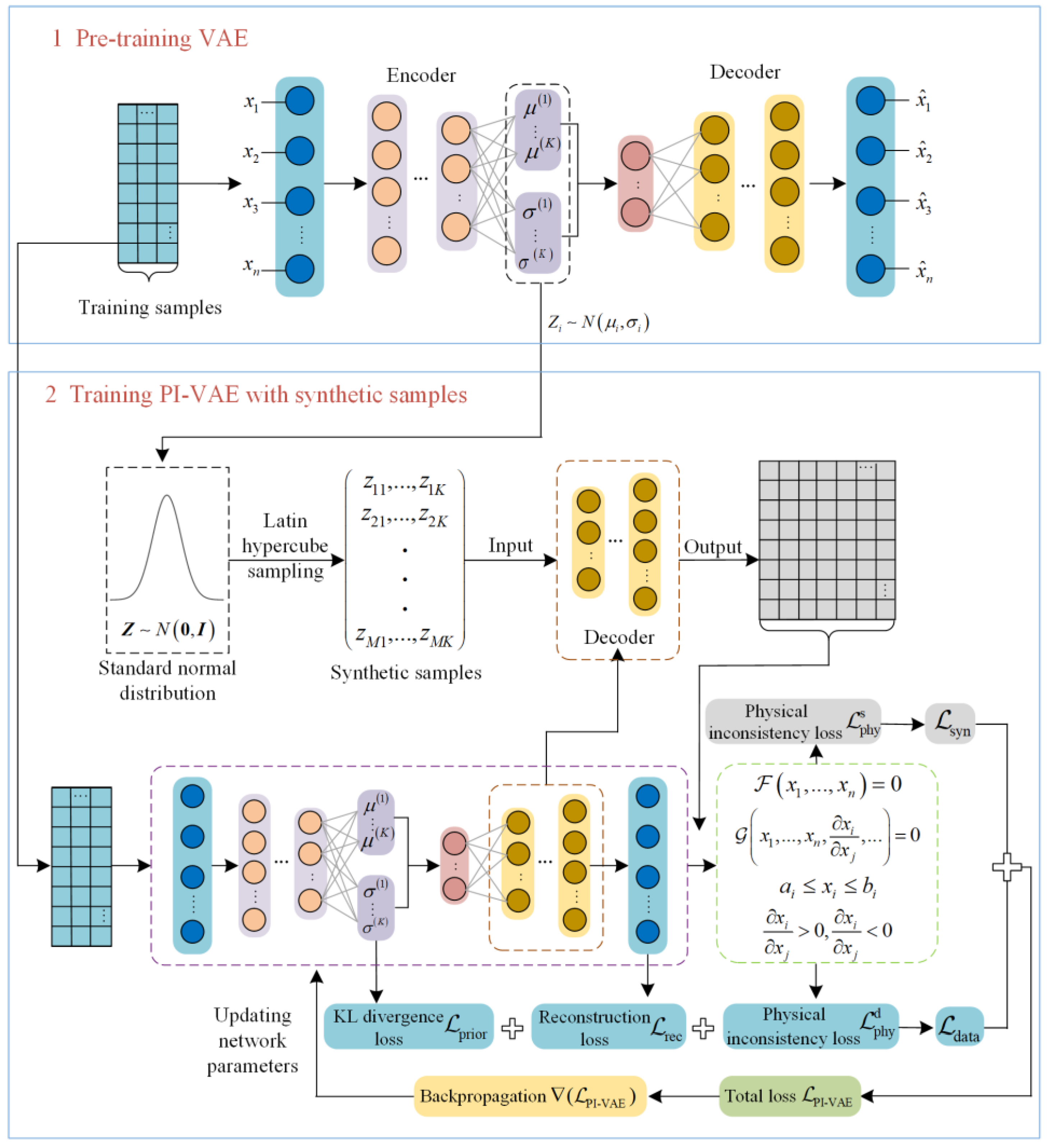
The training framework for the PI-VAE, illustrated in Figure 2, comprises two stages: VAE pre-training and PI-VAE training. In the VAE pre-training stage, a standard VAE model is constructed and trained using the training dataset ${\mathit{X}}_{\mathrm{d}\mathrm{a}\mathrm{t}\mathrm{a}}$. The training objective is to minimize the standard VAE loss ${\mathcal{L}}_{\mathrm{V}\mathrm{A}\mathrm{E}}$, which consists of reconstruction loss and KL divergence loss. This pre-training step initializes the encoder and decoder to learn a meaningful mapping between the data space and latent space. Subsequently, during the PI-VAE training stage, the pre-trained model is refined by incorporating physical knowledge. In this process, synthetic samples are generated by sampling the latent space using the LHS method, and these samples are then fed into the decoder to produce corresponding outputs. The model is trained using a joint dataset comprising both the training dataset ${\mathit{X}}_{\mathrm{d}\mathrm{a}\mathrm{t}\mathrm{a}}$ and the synthetic dataset ${\mathit{Z}}_{\mathrm{s}\mathrm{y}\mathrm{n}}$. The total loss function ${\mathcal{L}}_{\mathrm{P}\mathrm{I}-\mathrm{V}\mathrm{A}\mathrm{E}}$ is a composite of three terms: (i) the VAE loss ${\mathcal{L}}_{\mathrm{V}\mathrm{A}\mathrm{E}}$ calculated on training data; (ii) the physical inconsistency loss ${\mathcal{L}}_{\mathrm{p}\mathrm{h}\mathrm{y}}^{\mathrm{d}}$ calculated on the training data; and (iii) the physical inconsistency loss ${\mathcal{L}}_{\mathrm{p}\mathrm{h}\mathrm{y}}^{\mathrm{s}}$ calculated on outputs from the synthetic samples. By optimizing this composite loss, the network parameters are updated to produce results that are both accurate and physically consistent. The complete training procedure is outlined in Algorithm 2.

Algorithm 2. Training algorithm for the PI-VAE model

Input: normalized training dataset ${\mathit{X}}_{\mathrm{d}\mathrm{a}\mathrm{t}\mathrm{a}}$. Initialization: Randomly initialize network parameters $\mathit{\varphi }$ and $\mathit{\theta }.$ Given synthetic sample size $\mathit{M}$, batch size $m$, learning rate $\eta$, maximum number of iterations $E_1$ and $E_2$, weighting coefficients ${\alpha }_1$, ${\alpha }_2$ and $\beta$. VAE pre-training stage: Iteration For $\mathrm{e}\mathrm{p}\mathrm{o}\mathrm{c}\mathrm{h}=1 \mathrm{t}\mathrm{o} E_1$ do      Select a mini-batch $\mathit{X}$ from ${\mathit{X}}_{\mathrm{d}\mathrm{a}\mathrm{t}\mathrm{a}}$      Compute mean $\mathit{\mu }$ and variance ${\mathit{\sigma }}^2$ via the encoder: $(\mathit{\mu },{\mathit{\sigma }}^2){=E}_{\mathit{\varphi }}\left(\mathit{X}\right)$      Generate latent variable $\mathit{Z}$ using the reparameterization trick: $\mathit{z}=\mathit{\mu }+\mathit{\sigma }⨀\mathit{\epsilon }$, where $\mathit{\epsilon }~N(0,\mathit{I})$      Reconstruct $\mathit{X}$ via the decoder: $\widehat{\mathit{X}}=D_{\mathit{\theta }}\left(\mathit{Z}\right)$      Compute the VAE loss ${\mathcal{L}}_{\mathrm{v}\mathrm{a}\mathrm{e}}$ for $\mathit{X}$ using Equation (5)      Compute the gradient $-\nabla \left({\mathcal{L}}_{\mathrm{v}\mathrm{a}\mathrm{e}}\right)$ and update $\mathit{\varphi },\mathit{\theta }$ by descending the gradient Until ${\mathcal{L}}_{\mathrm{v}\mathrm{a}\mathrm{e}}$ converges, end the iteration. PI-VAE training stage:   Generate synthetic dataset ${\mathit{Z}}_{\mathrm{s}\mathrm{y}\mathrm{n}}$ using the sampling method from Algorithm 1. Iteration For $\mathrm{e}\mathrm{p}\mathrm{o}\mathrm{c}\mathrm{h}=1 \mathrm{t}\mathrm{o} E_2$ do      Select a mini-batch ${\mathit{X}}_1$ from ${\mathit{X}}_{\mathrm{d}\mathrm{a}\mathrm{t}\mathrm{a}}$      Reconstruct the training data batch to get ${\widehat{\mathit{X}}}_1=D_{\mathit{\theta }}\left(E_{\mathit{\varphi }}\right({\mathit{X}}_1\left)\right)$      Compute the VAE loss ${\mathcal{L}}_{\mathrm{v}\mathrm{a}\mathrm{e}}$ for ${\mathit{X}}_1$ using Equation (5)      Compute the physical inconsistency loss ${\mathcal{L}}_{\mathrm{p}\mathrm{h}\mathrm{y}}^{\mathrm{d}}$ on ${\widehat{\mathit{X}}}_1$ using Equation (27)      Select a mini-batch ${\mathit{Z}}_2$ from ${\mathit{Z}}_{\mathrm{s}\mathrm{y}\mathrm{n}}$      Obtain ${\widehat{\mathit{X}}}_2$ via the decoder: ${{\widehat{\mathit{X}}}_2=D}_{\mathit{\theta }}\left({\mathit{Z}}_2\right)$      Compute the physical inconsistency loss ${\mathcal{L}}_{\mathrm{p}\mathrm{h}\mathrm{y}}^{\mathrm{s}}$ on ${\widehat{\mathit{X}}}_2$ using Equation (29)      Compute the total PI-VAE loss: ${\mathcal{L}}_{\mathrm{P}\mathrm{I}-\mathrm{V}\mathrm{A}\mathrm{E}}={\mathcal{L}}_{\mathrm{V}\mathrm{A}\mathrm{E}}+{\alpha }_1{\mathcal{L}}_{\mathrm{p}\mathrm{h}\mathrm{y}}^{\mathrm{d}}+{{\alpha }_2\mathcal{L}}_{\mathrm{p}\mathrm{h}\mathrm{y}}^{\mathrm{s}}$      Compute the gradient $-\nabla \left({\mathcal{L}}_{\mathrm{P}\mathrm{I}-\mathrm{V}\mathrm{A}\mathrm{E}}\right)$ and update $\mathit{\varphi },\mathit{\theta }$ by descending the gradient Until ${\mathcal{L}}_{\mathrm{P}\mathrm{I}-\mathrm{V}\mathrm{A}\mathrm{E}}$ converges, end the iteration.

3. Results and Discussion

3.1. Numerical Case

The effectiveness of the proposed PI-VAE model is verified by a multivariable system with a strong nonlinear correlation between variables. This system can be given by:

$$\left\{\begin{array}{l}{x}_1=\gamma +e_1\\ x_2=0.3{\gamma }^2+0.5\gamma +e_2\\ x_3=0.4{\gamma }^2-1.6\gamma -0.4+e_3\\ x_4=-x_2+0.25+e_4\\ x_5={\gamma }^3+\cos {\gamma }^2+e_5\\ x_6=4\sin \gamma +0.4{\gamma }^3+\gamma +e_6\end{array}\right.$$

(31)

where $\gamma \sim U\left(\mathrm{0,3}\right)$ is drawn independently from the uniform distribution $U\left(\mathrm{0,3}\right)$, $e_i\sim N\left(0, 0.02\right), i=\mathrm{1,2},3\dots ,6$ is a collection of independent noise variables.

First, 20 samples are generated as training samples using Equation (31), with their distribution depicted in Figure 3. The observation reveals a significant data imbalance. Consider $x_1$, the interval [1, 2] contains no samples, while samples in the interval [2.5, 3.0] account for 60% of the total training dataset. Second, 2000 uniformly distributed test samples are generated using Equation (31).

3.1.1. Model Structure and Parameter Setting

To assess the performance of the proposed model, we compare the reconstruction accuracy of the PI-VAE model with that of the traditional VAE model. The hyperparameters for both models were determined using the Optuna hyperparameter search framework [42], and the specific parameter settings are provided in

Table 1. Network structure and hyperparameters for PIVAE and VAE models.

Model	Description	Value
PI-VAE	Network structure	6-16-8-2-8-16-6
	Activation function	“Relu”
	KL divergence loss weight $\beta$	0.1
	Physical inconsistency loss weight ${\alpha }_1$	0.1
	Physical inconsistency loss weight ${\alpha }_2$	0.2
	Optimizer	“Adam”
	Learning rate	0.001
	Batch size of training samples	100
	Maximum number of training iterations	5000
	Number of synthetic samples	500
VAE	Network structure	6-16-8-2-8-16-6
	Activation function	“Relu”
	KL divergence loss weight $\beta$	0.1
	Optimizer	“Adam”
	Learning rate	0.001
	Batch size of training samples	50
	Maximum number of training iterations	3000

. All computations were performed using Python 3.9 on a MacBook Pro with M1 Pro chipset (10-core CPU, 16-core GPU). To ensure a fair comparison, both the PI-VAE and VAE models have the same network structures and parameter configurations. The training process employs an early stopping mechanism to prevent overfitting and enhance computational efficiency.

Two widely used statistical metrics, the root mean square error (RMSE) and the coefficient of determination (R²), are used to quantitatively evaluate the performance of the models. The RMSE quantifies the average deviation between the predicted and measured values. It is calculated as follows:

$$\mathrm{R}\mathrm{M}\mathrm{S}\mathrm{E}=\sqrt{{\displaystyle \frac{1}{N}}{\sum }_{i=1}^N{\sum }_{j=1}^n{\left(x_j^{\left(i\right)}-{\widehat{x}}_j^{\left(i\right)}\right)}^2}$$

(32)

where $N$ denotes the number of samples, $n$ denotes the dimension of samples, $x_j^{\left(i\right)}$ and ${\widehat{x}}_j^{\left(i\right)}$ represnet the actual and predicted values of the $i$-th sample for the $j$-th variable, respectively.

The R² indicates how well the model fits the data, ranging from 0 to 1, with higher values representing a better fit. The R² is calculated as:

$${\mathrm{R}}^2=1-{\displaystyle \frac{\sum _{i=1}^N{{\sum }_{j=1}^n\left(x_j^{\left(i\right)}-{\widehat{x}}_j^{\left(i\right)}\right)}^2}{\sum _{i=1}^N{\sum }_{j=1}^n{\left(x_j^{\left(i\right)}-{\overline{x}}_j\right)}^2}}$$

(33)

where ${\overline{x}}_j$ denotes the mean of the actual values for the $j$-th variable.

3.1.2. Construction and Combination of Physical Constraints

To investigate how different physical constraints affect model performance, we developed a series of constraints for the six-dimensional nonlinear system described in Equation (31).

Table 2. Physical constraints on six-dimensional nonlinear systems.

No.	Mathematical Expression	Description
①	${\displaystyle \frac{\partial x_2}{\partial x_1}}>0$	Monotonicity
②	${\displaystyle \frac{\partial x_4}{\partial x_1}}<0$	Monotonicity
③	${\displaystyle \frac{\partial x_2}{\partial x_1}}-0.5-a{x}_1=0$	Incomplete partial differential equation
④	${\displaystyle \frac{\partial x_6}{\partial x_1}}-4\cos x_1-b{x}_1^2-1=0$	Incomplete partial differential equation
⑤	${\displaystyle \frac{\partial x_2}{\partial x_1}}-0.5-0.6x_1=0$	Partial differential equation
⑥	${\displaystyle \frac{\partial x_3}{\partial x_1}}-0.8x_1+1.6=0$	Partial differential equation
⑦	${\displaystyle \frac{\partial x_4}{\partial x_1}}+0.5+0.6x_1=0$	Partial differential equation
⑧	${\displaystyle \frac{\partial x_5}{\partial x_1}}-3x_1^2+2x_1\sin x_1^2=0$	Partial differential equation
⑨	${\displaystyle \frac{\partial x_6}{\partial x_1}}-4\cos x_1-1.2x_1^2-1=0$	Partial differential equation

presents the mathematical expressions for these constraints. They characterize relationships between system variables from various perspectives and can be categorized into three types: monotonicity constraints, incomplete differential equation constraints, and differential equation constraints. Notably, incomplete partial differential equations introduce unknown parameters, while partial differential equations provide explicit algebraic or transcendental functions, imposing stricter limitations on the variables. For a comprehensive performance comparison, we conducted a series of experiments by embedding different combinations of these constraints into the PI-VAE model. The specific constraint configurations are presented in

Table 3. Combination of physical constraints for six-dimensional nonlinear systems.

Model	Combination	Description
1	-	-
2	①	${\displaystyle \frac{\partial x_2}{\partial x_1}}>0$
3	①, ②	$\left\{\begin{array}{c}{\displaystyle \frac{\partial x_2}{\partial x_1}}>0\\ {\displaystyle \frac{\partial x_4}{\partial x_1}}<0\end{array}\right.$
4	③	${\displaystyle \frac{\partial x_2}{\partial x_1}}-0.5-a{x}_1=0$
5	③, ④	$\left\{\begin{array}{l}{\displaystyle \frac{\partial x_2}{\partial x_1}}-0.5-a{x}_1=0\\ {\displaystyle \frac{\partial x_6}{\partial x_1}}-4\cos x_1-b{x}_1^2-1=0\end{array}\right.$
6	⑤	${\displaystyle \frac{\partial x_2}{\partial x_1}}-0.5-0.6x_1=0$
7	⑤, ⑨	$\left\{\begin{array}{l}{\displaystyle \frac{\partial x_2}{\partial x_1}}-0.5-0.6x_1=0\\ {\displaystyle \frac{\partial x_6}{\partial x_1}}-4\cos x_1-1.2x_1^2-1=0\end{array}\right.$
8	⑤, ⑥, ⑨	$\left\{\begin{array}{l}{\displaystyle \frac{\partial x_2}{\partial x_1}}-0.5-0.6x_1=0\\ {\displaystyle \frac{\partial x_3}{\partial x_1}}-0.8x_1+1.6=0\\ {\displaystyle \frac{\partial x_6}{\partial x_1}}-4\cos x_1-1.2x_1^2-1=0\end{array}\right.$
9	⑤, ⑥, ⑦, ⑧, ⑨	$\left\{\begin{array}{l}{\displaystyle \frac{\partial x_2}{\partial x_1}}-0.5-0.6x_1=0\\ {\displaystyle \frac{\partial x_3}{\partial x_1}}-0.8x_1+1.6=0\\ {\displaystyle \frac{\partial x_4}{\partial x_1}}+0.5+0.6x_1=0\\ {\displaystyle \frac{\partial x_5}{\partial x_1}}-3x_1^2+2x_1\sin x_1^2=0\\ {\displaystyle \frac{\partial x_6}{\partial x_1}}-4\cos x_1-1.2x_1^2-1=0\end{array}\right.$

. The configuration without constraints corresponds to the standard VAE model.

3.1.3. Performance Analysis with Different Combinations of Physical Constraints

Following the constraint combinations specified in Table 3, corresponding PI-VAE and VAE models were trained, respectively. To assess performance robustness and reduce the impact of synthetic sample selection, each model configuration was independently trained 50 times.

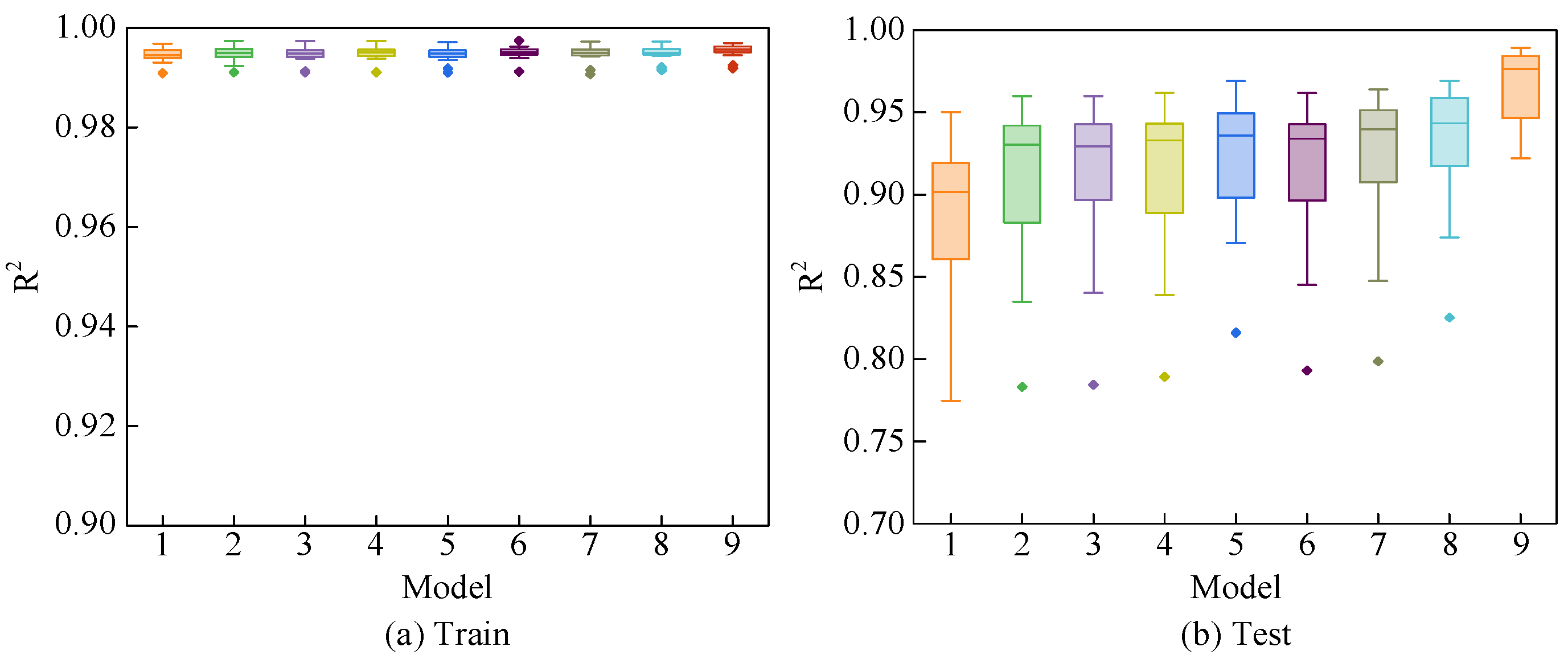
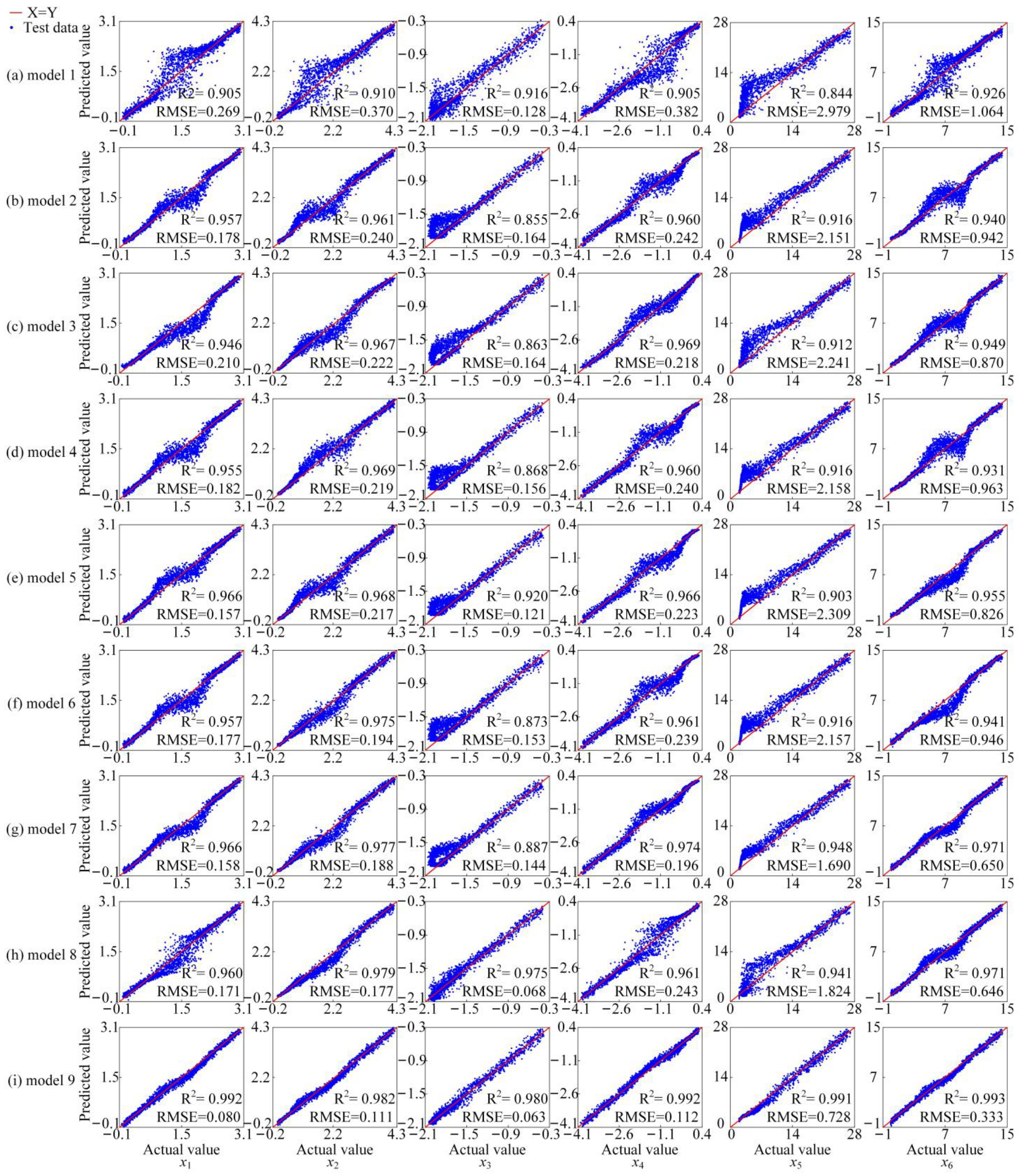
Figure 4 presents the prediction results for all models across both training and test datasets. As shown in Figure 4a, all models achieve high training accuracy, with median R² values exceeding 0.99. However, significant performance divergence was observed during testing (Figure 4b). The conventional VAE (model 1), which served as the unconstrained baseline, exhibited the poorest performance, yielding a median R² of 0.902 with considerable volatility. This highlights the limitations of this approach in scenarios with imbalanced data. Implementing monotonicity constraints (models 2 and 3) resulted in a notable improvement, raising the median R² to approximately 0.93 while significantly enhancing stability. Further enhancements were achieved by incorporating incomplete differential equations (models 4 and 5), which provided certain insights into parameter relationships and effectively reduced model uncertainty. Ultimately, the models that incorporated differential equation constraints (models 6–9) achieved the best results. Notably, model 9, which integrated five partial differential equations, reached the highest performance with a median R² of 0.976. This finding strongly indicates that comprehensive and accurate physical constraints are crucial for enhancing a PI-VAE model’s generalization capabilities. This conclusion is visually supported by the scatter plots for a representative trial (Figure 5), which illustrate a progressive improvement in test accuracy as more physical constraints are incorporated.

3.1.4. Performance Analysis with Different Synthetic Sample Sizes

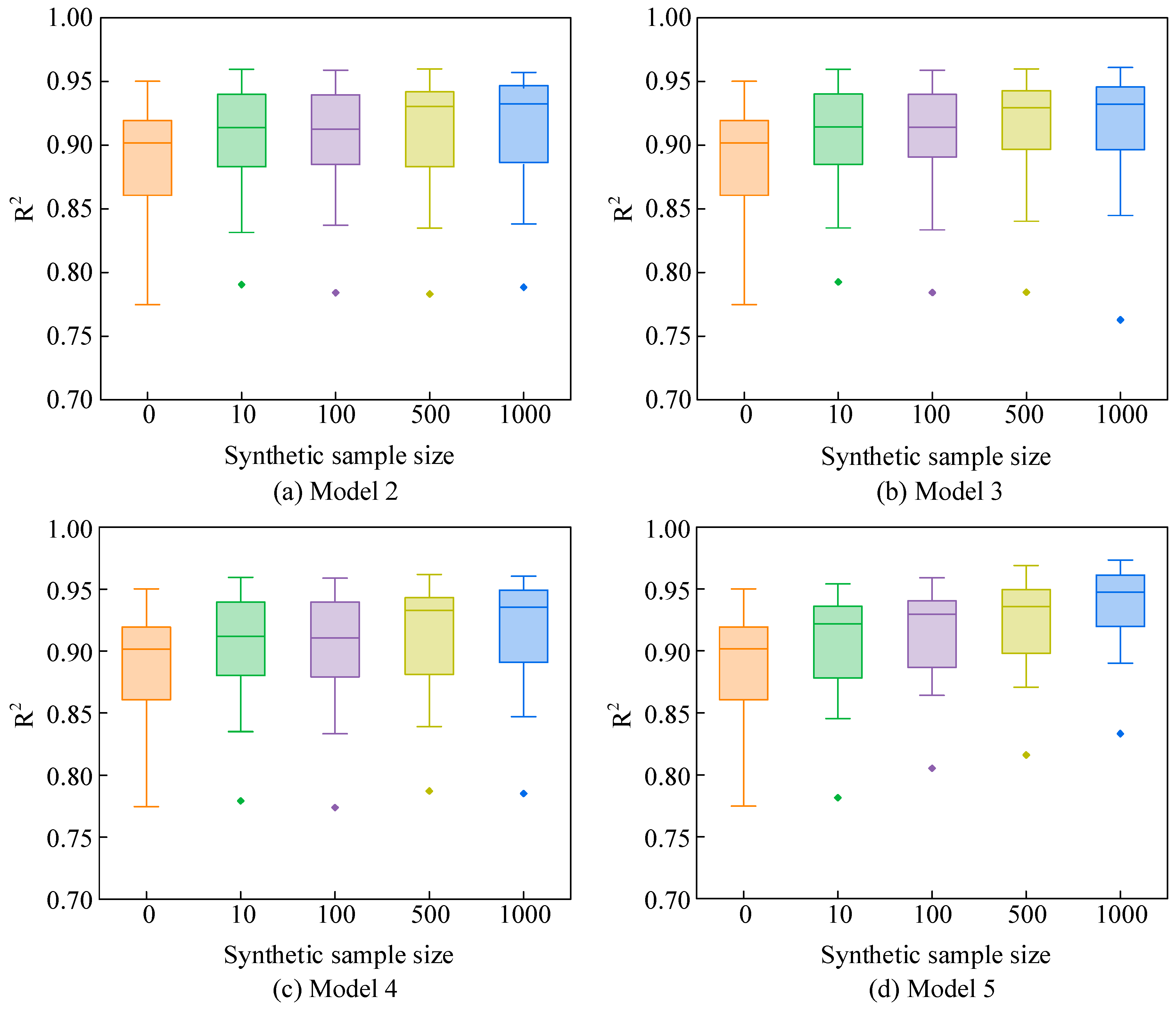
The size of synthetic samples is a crucial factor that influences the performance of the PI-VAE model. Figure 6 demonstrates how the synthetic sample size impacts test performance across various PI-VAE models. As shown, models 2 to 9 generally exhibit improvement in performance with an increasing number of synthetic samples. For the models that impose monotonicity constraints (models 2 and 3), the test performance increases rapidly with larger sample sizes before leveling off. However, models that integrate differential equation constraints (models 4–9) display a strong positive correlation between sample size and prediction performance. Specifically, in the case of model 9 with 1000 synthetic samples, the PI-VAE model achieves a median test R² of 0.983. This suggests that the required number of synthetic samples is influenced by the complexity of the embedded physical constraints. When complete physical constraints are used, a greater number of synthetic samples is necessary to improve the model’s generalization ability effectively. However, in scenarios where simplified constraints are applied, having too many synthetic samples can lead to an excess of redundant information, ultimately resulting in diminished performance gains.

The determination of synthetic sample size requires consideration of multiple factors, including the complexity of embedded physical constraints, data dimensionality, and system characteristics. Based on our experimental analysis, we recommend beginning with an empirically chosen synthetic sample size, then iteratively adjusting it based on validation performance metrics such as R² and constraint residual values. For systems with simple constraints (e.g., monotonicity only), smaller synthetic sample sizes may suffice, while systems with comprehensive differential equation constraints typically benefit from larger synthetic datasets to fully leverage the constraint guidance.

It is also important to consider the computational cost associated with the PI-VAE framework. The training time increases with the number and complexity of the physical constraints and the quantity of synthetic samples. For example, Model 9 with 1000 synthetic samples had an average training time of approximately 80 s over 50 runs, compared to approximately 5 s for the standard VAE. However, a significant advantage of the PI-VAE is that its inference time is nearly identical to that of a standard VAE, as it requires only a single forward pass through the network. This makes the trained model efficient and suitable for real-time applications.

3.2. HPFW System Case

3.2.1. Research Object and Model Training

The high-pressure feed water heater (HPFW) system is a crucial element in the thermal power plant, directly influencing the overall thermal efficiency [43]. Figure 7 illustrates the HPFW system of a 1000 MW coal-fired power plant. Its main components include three high-pressure feed water heaters (HPFW1, HPFW2, and HPFW3), a feed water pump (FWP), and a deaerator (DA).

Table 4. Primary operating parameters of the HPFW system.

No.	Variable	Description	Unit
1	$M_{\mathrm{F}\mathrm{F}\mathrm{W}}$	Outlet feed water mass flow rate of the HPFW1	t/h
2	$M_{\mathrm{F}\mathrm{W}\mathrm{P}}$	Outlet mass flow rate of the FWP	t/h
3	$M_{\mathrm{C}\mathrm{W}}$	Inlet condensate mass flow rate of the DA	t/h
4	$M_{\mathrm{D}\mathrm{A}}$	Outlet feed water mass flow rate of the DA	t/h
5	$P_{\mathrm{E}\mathrm{S}1}$	Extraction steam pressure to the HPFW1	MPa
6	$P_{\mathrm{E}\mathrm{S}2}$	Extraction steam pressure to the HPFW2	MPa
7	$P_{\mathrm{E}\mathrm{S}3}$	Extraction steam pressure to the HPFW3	MPa
8	$P_{\mathrm{E}\mathrm{S}4}$	Extraction steam pressure to the DA	MPa
9	$P_{\mathrm{C}\mathrm{W}}$	Inlet condensate pressure of the DA	MPa
10	$P_{\mathrm{F}\mathrm{W}\mathrm{P}}$	Outlet pressure of the FWP	MPa
11	$P_{\mathrm{H}\mathrm{P}\mathrm{F}\mathrm{W}3}$	Inlet pressure of the HPFW1	MPa
12	$P_{\mathrm{H}\mathrm{P}\mathrm{F}\mathrm{W}2}$	Inlet pressure of the HPFW2	MPa
13	$P_{\mathrm{H}\mathrm{P}\mathrm{F}\mathrm{W}1}$	Inlet pressure of the HPFW1	MPa
14	$P_{\mathrm{F}\mathrm{F}\mathrm{W}}$	Outlet pressure of the HPFW1	MPa
15	$T_{\mathrm{E}\mathrm{S}1}$	Extraction steam temperature of the HPFW1	°C
16	$T_{\mathrm{E}\mathrm{S}2}$	Extraction steam temperature of the HPFW2	°C
17	$T_{\mathrm{E}\mathrm{S}3}$	Extraction steam temperature of the HPFW3	°C
18	$T_{\mathrm{E}\mathrm{S}4}$	Extraction steam temperature of the DA	°C
19	$T_{\mathrm{C}\mathrm{W}}$	Inlet condensate temperature of the DA	°C
20	$T_{\mathrm{F}\mathrm{W}\mathrm{P}}$	Outlet temperature of the FWP	°C
21	$T_{\mathrm{H}\mathrm{P}\mathrm{F}\mathrm{W}3}$	Inlet feed water temperature of the HPFW3	°C
22	$T_{\mathrm{H}\mathrm{P}\mathrm{F}\mathrm{W}2}$	Inlet feed water temperature of the HPFW2	°C
23	$T_{\mathrm{H}\mathrm{P}\mathrm{F}\mathrm{W}1}$	Inlet feed water temperature of the HPFW1	°C
24	$T_{\mathrm{F}\mathrm{F}\mathrm{W}}$	Outlet temperature of the HPFW1	°C
25	$T_{\mathrm{D}\mathrm{W}1}$	Drain temperature of the HPFW1	°C
26	$T_{\mathrm{D}\mathrm{W}2}$	Drain temperature of the HPFW2	°C
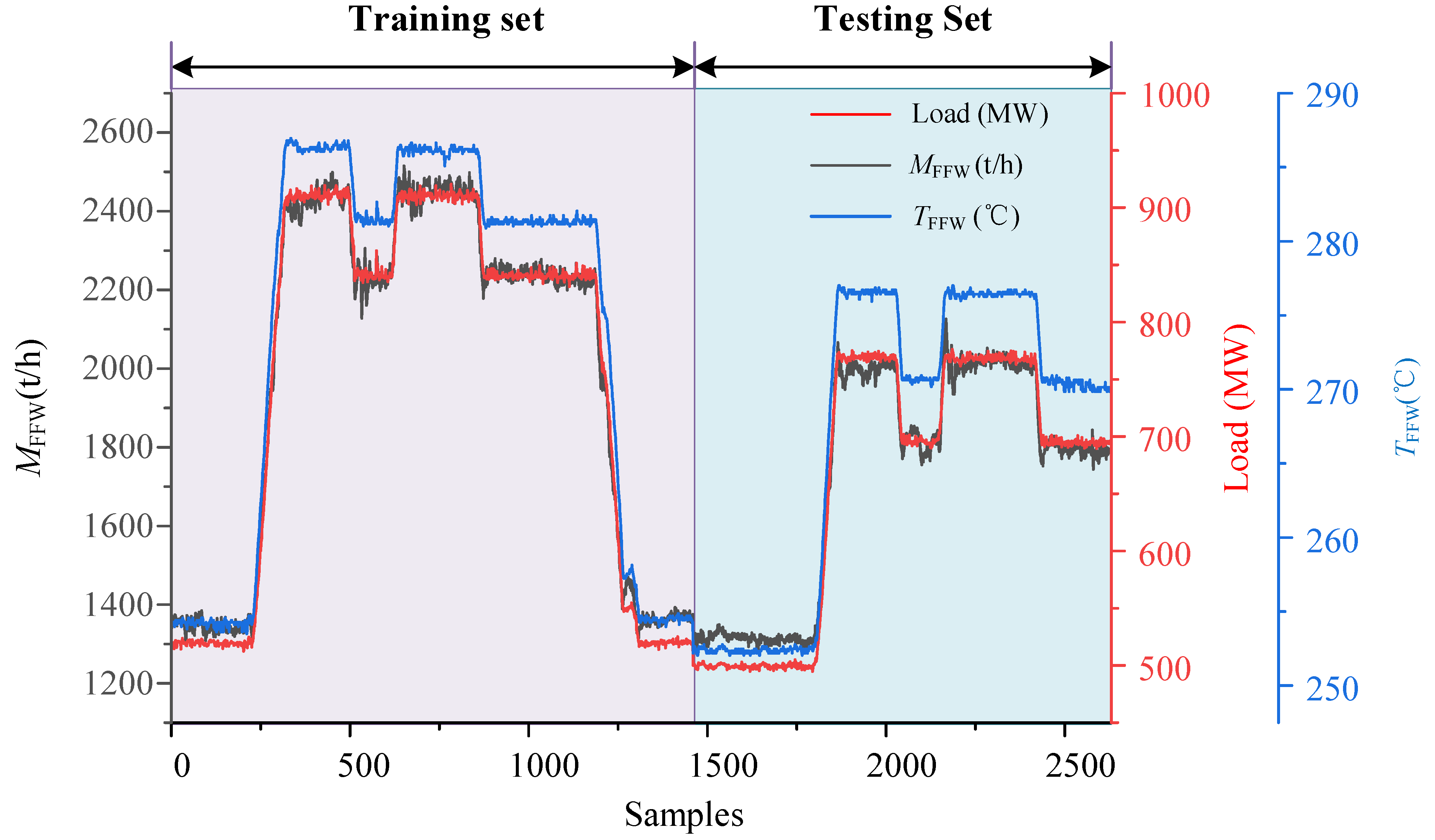
27	$T_{\mathrm{D}\mathrm{W}3}$	Drain temperature of the HPFW3	°C

presents key operating parameters of the HPFW system. A total of 2630 samples were collected at 60 s intervals from the plant’s Supervisory Information System (SIS) database. The first 1460 samples were used to create the training set, while the remaining 1170 samples comprised the test set. Figure 8 illustrates the historical trends of several operating parameters in both the training and test sets. Notably, there is a significant distributional discrepancy between these two sets. Specifically, the operating conditions in the test set differ from those covered by the training set. This divergence indicates that the model must possess strong extrapolation capabilities to perform effectively on the test set.

The PI-VAE model incorporates three categories of physical constraints, which are outlined in

Table 5. Physical constraints of the HPFW system.

Device	No.	Physical Constraint Expression	Description
HPFW1	①	$M_{\mathrm{E}\mathrm{S}1}-M_{\mathrm{D}\mathrm{W}1}=0$	Mass balance
	②	$M_{\mathrm{F}\mathrm{F}\mathrm{W}}\cdot h\left(P_{\mathrm{H}\mathrm{P}\mathrm{F}\mathrm{W}1},T_{\mathrm{H}\mathrm{P}\mathrm{F}\mathrm{W}1}\right)+M_{\mathrm{E}\mathrm{S}1}\cdot h\left(P_{\mathrm{E}\mathrm{S}1},T_{\mathrm{E}\mathrm{S}1}\right)-M_{\mathrm{F}\mathrm{F}\mathrm{W}}\cdot h\left(P_{\mathrm{F}\mathrm{F}\mathrm{W}},T_{\mathrm{F}\mathrm{F}\mathrm{W}}\right)$$-M_{\mathrm{D}\mathrm{W}1}\cdot h\left(P_{\mathrm{E}\mathrm{S}1},T_{\mathrm{D}\mathrm{W}1}\right)=0$	Energy balance
	③	${\displaystyle \frac{\partial P_{\mathrm{H}\mathrm{P}\mathrm{F}\mathrm{W}2}}{\partial P_{\mathrm{H}\mathrm{P}\mathrm{F}\mathrm{W}1}}}>0$	Monotonicity
HPFW2	①	$M_{\mathrm{E}\mathrm{S}2}+M_{\mathrm{D}\mathrm{W}1}-M_{\mathrm{D}\mathrm{W}2}=0$	Mass balance
	②	$M_{\mathrm{F}\mathrm{F}\mathrm{W}}\cdot h\left(P_{\mathrm{H}\mathrm{P}\mathrm{F}\mathrm{W}2},T_{\mathrm{H}\mathrm{P}\mathrm{F}\mathrm{W}2}\right)+M_{\mathrm{E}\mathrm{S}2}\cdot h\left(P_{\mathrm{E}\mathrm{S}2},T_{\mathrm{E}\mathrm{S}2}\right)+M_{\mathrm{D}\mathrm{W}1}\cdot h\left(P_{\mathrm{E}\mathrm{S}1},T_{\mathrm{D}\mathrm{W}1}\right)$$-M_{\mathrm{F}\mathrm{F}\mathrm{W}}\cdot h\left(P_{\mathrm{H}\mathrm{P}\mathrm{F}\mathrm{W}1},T_{\mathrm{H}\mathrm{P}\mathrm{F}\mathrm{W}1}\right)-M_{\mathrm{D}\mathrm{W}2}\cdot h\left(P_{\mathrm{E}\mathrm{S}2},T_{\mathrm{D}\mathrm{W}2}\right)=0$	Energy balance
	③	${\displaystyle \frac{\partial P_{\mathrm{H}\mathrm{P}\mathrm{F}\mathrm{W}3}}{\partial P_{\mathrm{H}\mathrm{P}\mathrm{F}\mathrm{W}2}}}>0$	Monotonicity
HPFW3	①	$M_{\mathrm{E}\mathrm{S}3}+M_{\mathrm{D}\mathrm{W}2}-M_{\mathrm{D}\mathrm{W}3}=0$	Mass balance
	②	$M_{\mathrm{F}\mathrm{F}\mathrm{W}}\cdot h\left(P_{\mathrm{H}\mathrm{P}\mathrm{F}\mathrm{W}3},T_{\mathrm{H}\mathrm{P}\mathrm{F}\mathrm{W}3}\right)+M_{\mathrm{E}\mathrm{S}3}\cdot h\left(P_{\mathrm{E}\mathrm{S}3},T_{\mathrm{E}\mathrm{S}3}\right)+M_{\mathrm{D}\mathrm{W}2}\cdot h\left(P_{\mathrm{E}\mathrm{S}2},T_{\mathrm{D}\mathrm{W}2}\right)$$-M_{\mathrm{F}\mathrm{F}\mathrm{W}}\cdot h\left(P_{\mathrm{H}\mathrm{P}\mathrm{F}\mathrm{W}2},T_{\mathrm{H}\mathrm{P}\mathrm{F}\mathrm{W}2}\right)-M_{\mathrm{D}\mathrm{W}3}\cdot h\left(P_{\mathrm{E}\mathrm{S}3},T_{\mathrm{D}\mathrm{W}3}\right)=0$	Energy balance
FWP	①	$M_{\mathrm{F}\mathrm{F}\mathrm{W}}-M_{\mathrm{F}\mathrm{W}\mathrm{P}}=0$	Mass balance
	②	${\displaystyle \frac{\partial P_{\mathrm{F}\mathrm{W}\mathrm{P}}}{\partial P_{\mathrm{H}\mathrm{P}\mathrm{F}\mathrm{W}3}}}>0$	Monotonicity
	③	${\displaystyle \frac{\partial P_{\mathrm{F}\mathrm{W}\mathrm{P}}}{\partial P_{\mathrm{H}\mathrm{P}\mathrm{F}\mathrm{W}2}}}>0$	Monotonicity
	④	${\displaystyle \frac{\partial P_{\mathrm{F}\mathrm{W}\mathrm{P}}}{\partial P_{\mathrm{H}\mathrm{P}\mathrm{H}1}}}>0$	Monotonicity
	⑤	${\displaystyle \frac{\partial P_{\mathrm{F}\mathrm{W}\mathrm{P}}}{\partial P_{\mathrm{F}\mathrm{F}\mathrm{W}}}}>0$	Monotonicity
DA	①	$M_{\mathrm{E}\mathrm{S}4}+M_{\mathrm{C}\mathrm{W}}+M_{\mathrm{D}\mathrm{W}3}-M_{\mathrm{D}\mathrm{A}}=0$	Mass balance
	②	$M_{\mathrm{E}\mathrm{S}4}\cdot h\left(P_{\mathrm{E}\mathrm{S}4},T_{\mathrm{E}\mathrm{S}4}\right)+M_{\mathrm{C}\mathrm{W}}\cdot h\left(P_{\mathrm{C}\mathrm{W}},T_{\mathrm{C}\mathrm{W}}\right){+M}_{\mathrm{D}\mathrm{W}3}\cdot h\left(P_{\mathrm{E}\mathrm{S}3},T_{\mathrm{D}\mathrm{W}3}\right)$$-M_{\mathrm{D}\mathrm{A}}\cdot h_{\mathrm{s}\mathrm{a}\mathrm{t},\mathrm{w}}\left(P_{\mathrm{E}\mathrm{S}4}\right)=0$	Energy balance

. These constraints are based on fundamental physical laws governing the HPFW system [44] and include mass conservation equations, energy conservation equations, and monotonic relationships. The thermodynamic parameters for water and steam are calculated in strict accordance with the IAPWS-IF97 standard [44]. In the notation used, $h(P,T)$ represents the specific enthalpy at a given pressure $P$ and temperature $T$, while $h_{\mathrm{s}\mathrm{a}\mathrm{t},\mathrm{w}}\left(P\right)$ denotes the specific enthalpy of saturated water at pressure $P$. To simplify the physical constraint equations, two key assumptions were made: (1) pressure losses during fluid flow are considered negligible, and (2) heat losses from the extraction steam pipelines and the heaters themselves are not considered. It is also important to note that implementing these physical constraints requires the introduction of several unmeasurable auxiliary parameters, which are specified in

Table 6. Unmeasurable auxiliary parameters in physical constraints.

Variable	Description	Unit
$M_{\mathrm{E}\mathrm{S}1}$	Extraction steam mass flow rate to the HPFW1	t/h
$M_{\mathrm{E}\mathrm{S}2}$	Extraction steam mass flow rate to the HPFW2	t/h
$M_{\mathrm{E}\mathrm{S}3}$	Extraction steam mass flow rate to the HPFW3	t/h
$M_{\mathrm{E}\mathrm{S}4}$	Extraction steam mass flow rate to the deaerator	t/h
$M_{\mathrm{D}\mathrm{W}1}$	Drain mass flow rate of the HPFW1	t/h
$M_{\mathrm{D}\mathrm{W}2}$	Drain mass flow rate of the HPFW2	t/h
$M_{\mathrm{D}\mathrm{W}3}$	Drain mass flow rate of the HPFW3	t/h

.

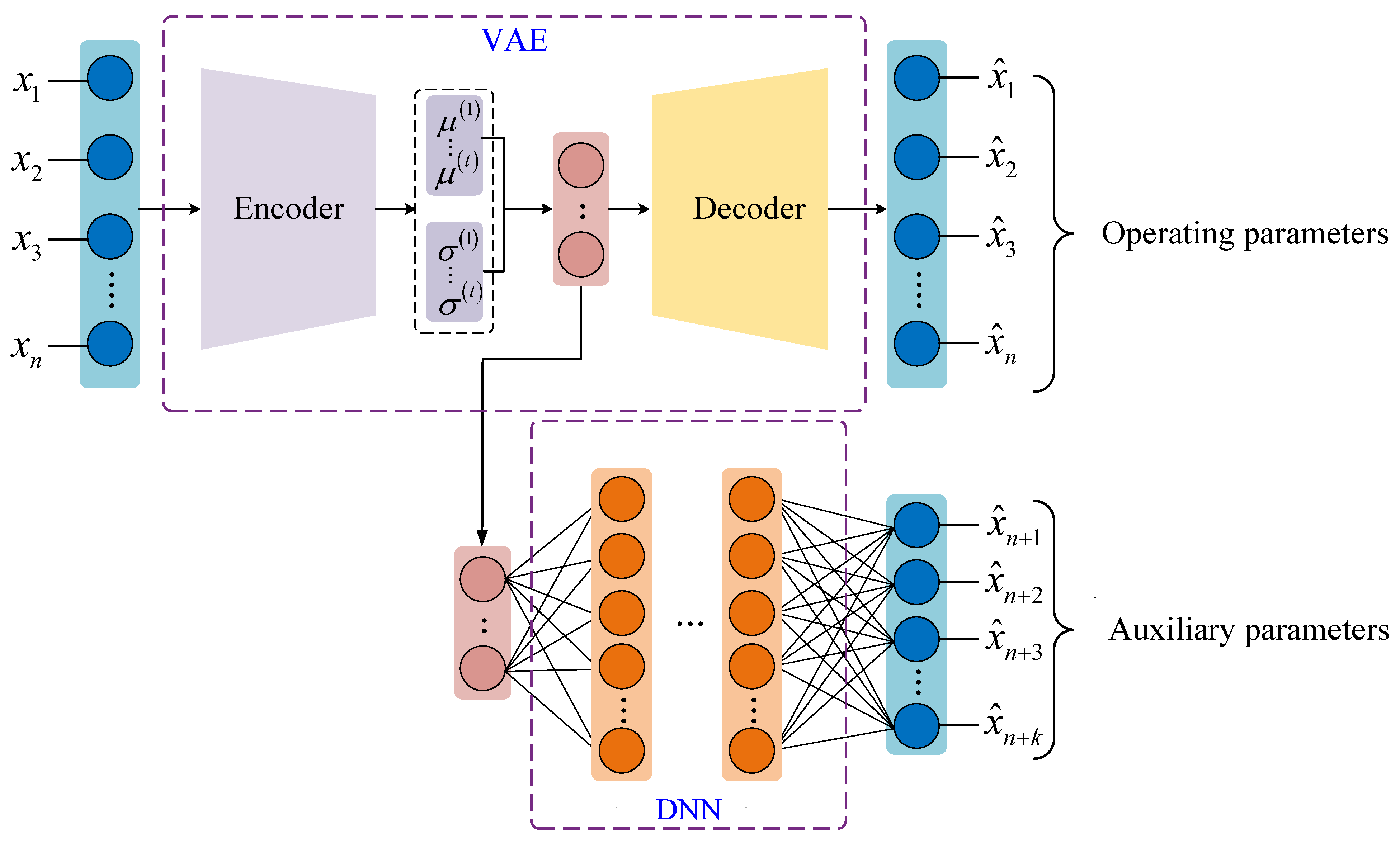
This work establishes two models for comparison: a baseline VAE model and a PI-VAE model. The architecture of the PI-VAE model, as illustrated in Figure 9, extends the standard VAE by integrating an additional deep neural network (DNN). A key aspect of the PI-VAE training procedure is that the auxiliary parameters, listed in Table 6, are solely utilized to compute the physical inconsistency loss and do not contribute to the reconstruction loss. To ensure a fair comparison between the PI-VAE and VAE models, both are configured with identical encoder and decoder network structures. The hyperparameter settings for the two models are provided in

Table 7. Model Configurations of PI-VAE and VAE for HPFW system modeling.

Model	Descriptions	Value
PI-VAE	VAE network structure	27-40-15-5-15-40-27
	DNN structure	5-10-20-7
	Activation function	“Relu”
	KL divergence loss weight $\beta$	0.1
	Physical inconsistency loss weight ${\alpha }_1$	0.002
	Physical inconsistency loss weight ${\alpha }_2$	0.003
	Optimizer	“Adam”
	Learning rate	0.001
	Batch size of training samples	500
	Maximum number of training iterations	5000
	Number of synthetic samples	2000
VAE	Network structure	27-40-15-5-15-40-27
	Activation function	“Relu”
	KL divergence loss weight $\beta$	0.1
	Optimizer	“Adam”
	Learning rate	0.001
	Batch size of training samples	500
	Maximum number of training iterations	3000

.

3.2.2. Model Performance Analysis

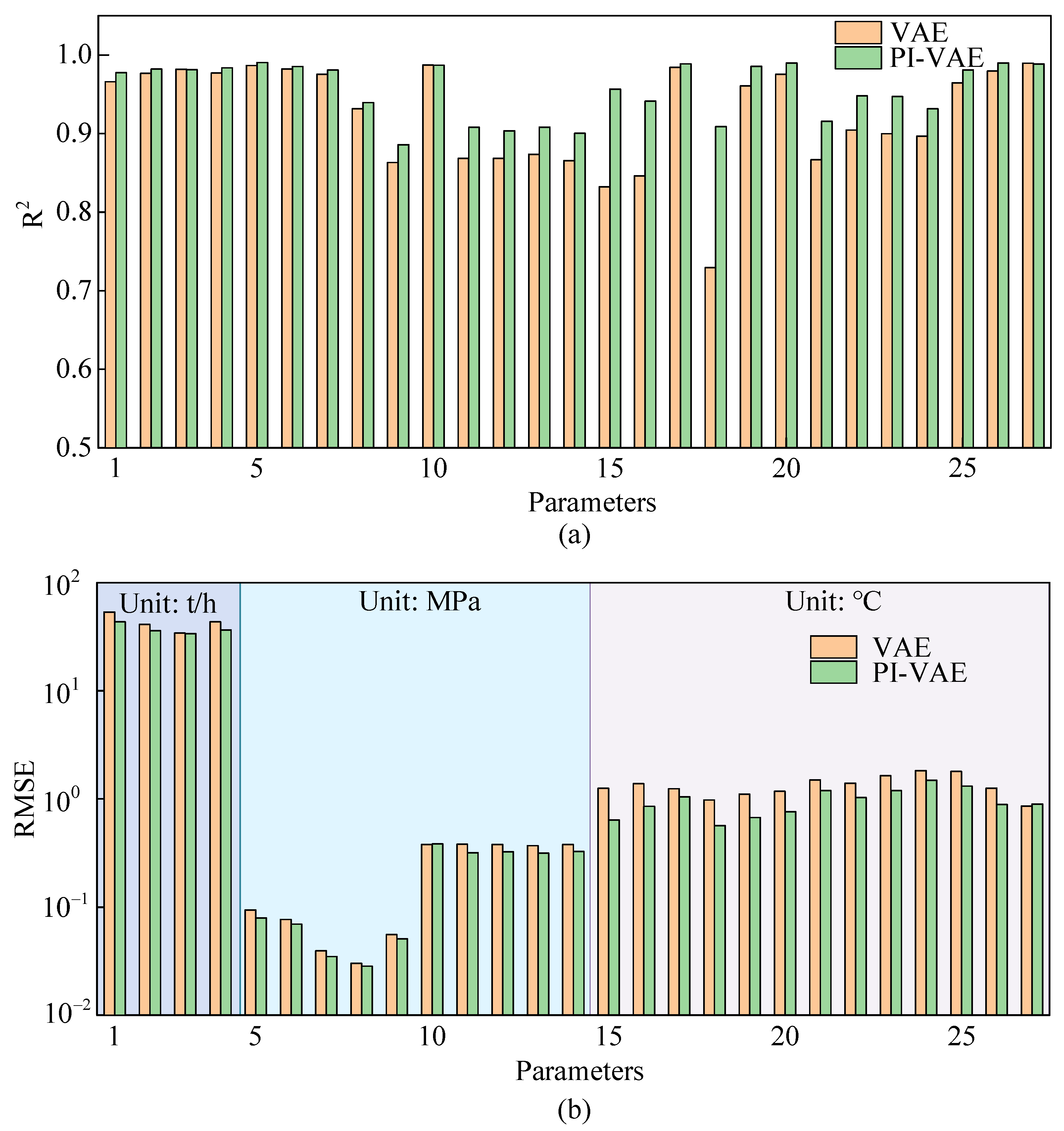
In the training set, both the VAE and PI-VAE models exhibited high fitting accuracy, with average R² values of 0.994 and 0.991, respectively. However, their performance on the test set, as illustrated in Figure 10, revealed a noticeable divergence. The results indicate that the PI-VAE model achieves superior test accuracy across various operating parameters compared to the standard VAE. This strongly suggests that incorporating physical constraints enhances the model’s ability to generalize and improves its predictive accuracy under unseen operating conditions.

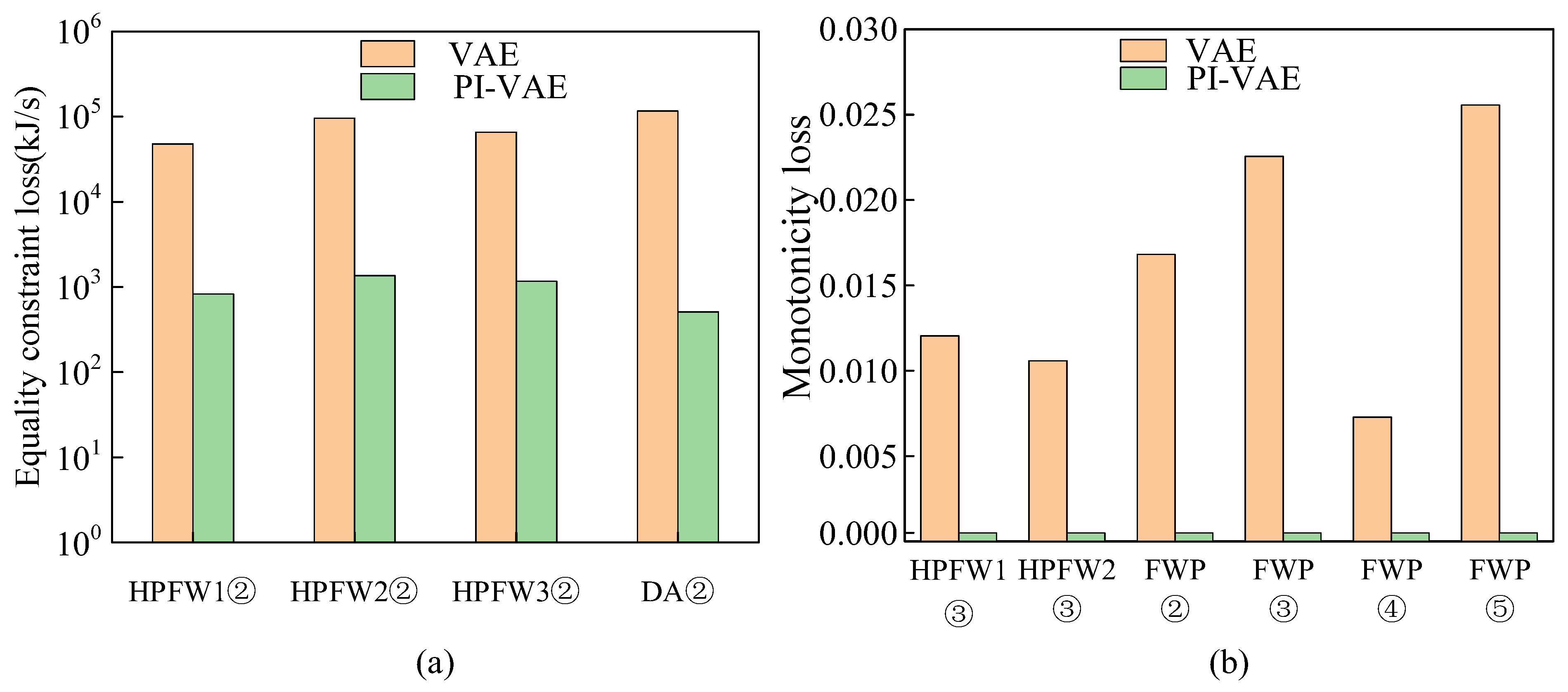
To further evaluate the physical consistency of the models on the test set, we examined them using both equality constraint loss and monotonicity loss. For the equality constraints, using the four energy conservation equations from Table 5 as an example, Figure 11a shows that the PI-VAE significantly outperforms the standard VAE. It is important to note that the constraint loss for the PI-VAE does not reach zero under actual operating conditions. This is due to intentional simplifications made in the embedded physical equations. Regarding the monotonicity constraints, the results displayed in Figure 11b reveal an even more significant contrast. The PI-VAE model perfectly adheres to all the monotonicity conditions defined in Table 5, while the VAE model violates all six conditions to varying extents. Overall, these findings provide strong evidence that the PI-VAE not only fits the data well but also learns and generalizes the underlying physical principles, ensuring its predictions remain physically consistent under new operating conditions.

4. Conclusions

To address the challenges of poor interpretability and limited generalization in traditional data-driven models, this study introduces a PI-VAE approach for modeling thermal systems. The approach begins by formalizing the fundamental principles governing thermal systems into a comprehensive framework of physical constraints, which includes algebraic equations, partial differential equations, boundary conditions, and monotonic relationships. These constraints are then transformed into corresponding physical inconsistency losses to guide the training process of the model. Additionally, a strategy for generating synthetic samples based on latent variable sampling is developed to broaden the coverage of these physical constraints.

The effectiveness of the PI-VAE approach is validated through numerical experiments conducted on a nonlinear system. The results indicate that increasing the diversity of physical constraints continuously improves model accuracy. There is a positive correlation between the size of the synthetic sample and the strength of the physical constraints; however, adding redundant synthetic samples does not lead to further performance improvements. Using a HPFW system in a thermal power plant as a case study, a PI-VAE model that incorporates mass conservation, energy conservation, and monotonicity constraints is developed. The results confirm that integrating physical principles into the data-driven model significantly enhances both its generalization capability and interpretability, effectively addressing the modeling challenges posed by imbalanced training data distributions.

Future work will focus on extending the proposed framework to address dynamic systems. The current study focuses on static modeling, which does not fully capture the time-varying characteristics of thermal systems. Therefore, a promising direction is integrating the PI-VAE with sequential modeling architectures, such as long short-term memory (LSTM) networks or transformers, to model dynamic processes in thermal systems.

References

1. Ge, Z. Review on data-driven modeling and monitoring for plant-wide industrial processes. Chemom. Intell. Lab. Syst. 2017, 171, 16–25. [Google Scholar] [CrossRef]
2. Ren, S.; Jin, Y.; Zhao, J.; Cao, Y.; Si, F. Nonlinear process monitoring based on generic reconstruction-based auto-associative neural network. J. Frankl. Inst. 2023, 360, 5149–5170. [Google Scholar] [CrossRef]
3. Zhu, Y.; Yu, C.; Jin, W.; Shi, L.; Chen, B.; Xu, P. Mechanism-enhanced data-driven method for the joint optimization of boiler combustion and selective catalytic reduction systems considering gas temperature deviations. Energy 2024, 291, 130432. [Google Scholar] [CrossRef]
4. Zhou, D.; Huang, D. A review on the progress, challenges and prospects in the modeling, simulation, control and diagnosis of thermodynamic systems. Adv. Eng. Inform. 2024, 60, 102435. [Google Scholar] [CrossRef]
5. Chen, C.; Liu, M.; Li, M.; Wang, Y.; Wang, C.; Yan, J. Digital twin modeling and operation optimization of the steam turbine system of thermal power plants. Energy 2024, 290, 129969. [Google Scholar] [CrossRef]
6. Zhang, S.; Zhao, C. Concurrent analysis of variable correlation and data distribution for monitoring large-scale processes under varying operation conditions. Neurocomputing 2019, 349, 225–238. [Google Scholar] [CrossRef]
7. Chang, J.; Wang, X.; Zhou, Z.; Chen, H.; Niu, Y. CFD modeling of hydrodynamics, combustion and NOx emission in a tangentially fired pulverized-coal boiler at low load operating conditions. Adv. Powder Technol. 2021, 32, 290–303. [Google Scholar] [CrossRef]
8. Yang, Y.; Nikolaidis, T.; Jafari, S.; Pilidis, P. Gas turbine engine transient performance and heat transfer effect modelling: A comprehensive review, research challenges, and exploring the future. Appl. Therm. Eng. 2024, 236, 121523. [Google Scholar] [CrossRef]
9. Wang, J.; Feng, Y.; Ye, S.; Zhang, Y.; Ma, Z.; Dong, F. NOx emission prediction of coal-fired power units under uncertain classification of operating conditions. Fuel 2023, 343, 127840. [Google Scholar] [CrossRef]
10. Song, H.; Liu, X.; Song, M. Comparative study of data-driven and model-driven approaches in prediction of nuclear power plants operating parameters. Appl. Energy 2023, 341, 121077. [Google Scholar] [CrossRef]
11. Fenza, G.; Gallo, M.; Loia, V.; Orciuoli, F.; Herrera-Viedma, E. Data set quality in Machine Learning: Consistency measure based on Group Decision Making. Appl. Soft Comput. 2021, 106, 107366. [Google Scholar] [CrossRef]
12. Lv, Y.; Romero, C.E.; Yang, T.; Fang, F.; Liu, J. Typical condition library construction for the development of data-driven models in power plants. Appl. Therm. Eng. 2018, 143, 160–171. [Google Scholar] [CrossRef]
13. Vabalas, A.; Gowen, E.; Poliakoff, E.; Casson, A.J. Machine learning algorithm validation with a limited sample size. PLoS ONE 2019, 14, e0224365. [Google Scholar] [CrossRef]
14. Azodi, C.B.; Tang, J.; Shiu, S.-H. Opening the Black Box: Interpretable Machine Learning for Geneticists. Trends Genet. 2020, 36, 442–455. [Google Scholar] [CrossRef]
15. Bradley, W.; Kim, J.; Kilwein, Z.; Blakely, L.; Eydenberg, M.; Jalvin, J.; Laird, C.; Boukouvala, F. Perspectives on the integration between first-principles and data-driven modeling. Comput. Chem. Eng. 2022, 166, 107898. [Google Scholar] [CrossRef]
16. Soofi, Y.J.; Gu, Y.; Liu, J. An adaptive Physics-based feature engineering approach for Machine Learning-assisted alloy discovery. Comput. Mater. Sci. 2023, 226, 112248. [Google Scholar] [CrossRef]
17. Zhu, H.; Tsang, E.C.C.; Wang, X.-Z.; Aamir Raza Ashfaq, R. Monotonic classification extreme learning machine. Neurocomputing 2017, 225, 205–213. [Google Scholar] [CrossRef]
18. Pan, C.; Dong, Y.; Yan, X.; Zhao, W. Hybrid model for main and side reactions of p-xylene oxidation with factor influence based monotone additive SVR. Chemom. Intell. Lab. Syst. 2014, 136, 36–46. [Google Scholar] [CrossRef]
19. Ji, W.; Deng, S. Autonomous Discovery of Unknown Reaction Pathways from Data by Chemical Reaction Neural Network. J. Phys. Chem. A 2021, 125, 1082–1092. [Google Scholar] [CrossRef] [PubMed]
20. Ji, W.; Richter, F.; Gollner, M.J.; Deng, S. Autonomous kinetic modeling of biomass pyrolysis using chemical reaction neural networks. Combust. Flame 2022, 240, 111992. [Google Scholar] [CrossRef]
21. Raissi, M.; Yazdani, A.; Karniadakis, G.E. Hidden fluid mechanics: Learning velocity and pressure fields from flow visualizations. Science 2020, 367, 1026–1030. [Google Scholar] [CrossRef]
22. Karniadakis, G.E.; Kevrekidis, I.G.; Lu, L.; Perdikaris, P.; Wang, S.; Yang, L. Physics-informed machine learning. Nat. Rev. Phys. 2021, 3, 422–440. [Google Scholar] [CrossRef]
23. Wu, Y.; Sicard, B.; Gadsden, S.A. Physics-informed machine learning: A comprehensive review on applications in anomaly detection and condition monitoring. Expert Syst. Appl. 2024, 255, 124678. [Google Scholar] [CrossRef]
24. Cuomo, S.; Di Cola, V.S.; Giampaolo, F.; Rozza, G.; Raissi, M.; Piccialli, F. Scientific Machine Learning Through Physics–Informed Neural Networks: Where we are and What’s Next. J. Sci. Comput. 2022, 92, 88. [Google Scholar] [CrossRef]
25. Cai, S.Z.; Mao, Z.P.; Wang, Z.C.; Yin, M.L.; Karniadakis, G.E. Physics-informed neural networks (PINNs) for fluid mechanics: A review. Acta Mech. Sin. 2021, 37, 1727–1738. [Google Scholar] [CrossRef]
26. Jalili, D.; Jang, S.; Jadidi, M.; Giustini, G.; Keshmiri, A.; Mahmoudi, Y. Physics-informed neural networks for heat transfer prediction in two-phase flows. Int. J. Heat Mass Transf. 2024, 221, 125089. [Google Scholar] [CrossRef]
27. Alber, M.; Buganza Tepole, A.; Cannon, W.R.; De, S.; Dura-Bernal, S.; Garikipati, K.; Karniadakis, G.; Lytton, W.W.; Perdikaris, P.; Petzold, L.; et al. Integrating machine learning and multiscale modeling—Perspectives, challenges, and opportunities in the biological, biomedical, and behavioral sciences. npj Digit. Med. 2019, 2, 115. [Google Scholar] [CrossRef]
28. Zideh, M.J.; Chatterjee, P.; Srivastava, A.K. Physics-Informed Machine Learning for Data Anomaly Detection, Classification, Localization, and Mitigation: A Review, Challenges, and Path Forward. IEEE Access 2024, 12, 4597–4617. [Google Scholar] [CrossRef]
29. Raissi, M.; Perdikaris, P.; Karniadakis, G.E. Physics-informed neural networks: A deep learning framework for solving forward and inverse problems involving nonlinear partial differential equations. J. Comput. Phys. 2019, 378, 686–707. [Google Scholar] [CrossRef]
30. Haghighat, E.; Raissi, M.; Moure, A.; Gomez, H.; Juanes, R. A physics-informed deep learning framework for inversion and surrogate modeling in solid mechanics. Comput. Methods Appl. Mech. Eng. 2021, 379, 113741. [Google Scholar] [CrossRef]
31. Li, P.; Pei, Y.; Li, J. A comprehensive survey on design and application of autoencoder in deep learning. Appl. Soft Comput. 2023, 138, 110176. [Google Scholar] [CrossRef]
32. Chen, X.; Zhao, C. Conditional discriminative autoencoder and condition-driven immediate representation of soft transition for monitoring complex nonstationary processes. Control Eng. Pract. 2022, 122, 105090. [Google Scholar] [CrossRef]
33. Kim, H.; Ko, J.U.; Na, K.; Lee, H.; Kim, H.-S.; Son, J.-D.; Yoon, H.; Youn, B.D. Opt-TCAE: Optimal temporal convolutional auto-encoder for boiler tube leakage detection in a thermal power plant using multi-sensor data. Expert Syst. Appl. 2023, 215, 119377. [Google Scholar] [CrossRef]
34. Khalid Fahmi, A.-T.W.; Reza Kashyzadeh, K.; Ghorbani, S. Fault detection in the gas turbine of the Kirkuk power plant: An anomaly detection approach using DLSTM-Autoencoder. Eng. Fail. Anal. 2024, 160, 108213. [Google Scholar] [CrossRef]
35. Alemi, A.; Poole, B.; Fischer, I.; Dillon, J.; Saurous, R.A.; Murphy, K. Fixing a Broken ELBO. In Proceedings of the 35th International Conference on Machine Learning; Proceedings of Machine Learning Research; Stockholmsmässan, Stockholm Sweden; 10–15 July 2018; Jennifer, D., Andreas, K., Eds.; PMLR: Cambridge, MA, USA, 2018; Volume 80, pp. 159–168. [Google Scholar]
36. Kingma, D.P.; Welling, M. An introduction to variational autoencoders. Found. Trends® Mach. Learn. 2019, 12, 307–392. [Google Scholar] [CrossRef]
37. Styan, G.P.H. Hadamard products and multivariate statistical analysis. Linear Algebra Its Appl. 1973, 6, 217–240. [Google Scholar] [CrossRef]
38. Margossian, C.C. A review of automatic differentiation and its efficient implementation. WIREs Data Min. Knowl. Discov. 2019, 9, e1305. [Google Scholar] [CrossRef]
39. Wu, C.; Zhu, M.; Tan, Q.; Kartha, Y.; Lu, L. A comprehensive study of non-adaptive and residual-based adaptive sampling for physics-informed neural networks. Comput. Methods Appl. Mech. Eng. 2023, 403, 115671. [Google Scholar] [CrossRef]
40. Sholokhov, A.; Liu, Y.; Mansour, H.; Nabi, S. Physics-informed neural ODE (PINODE): Embedding physics into models using collocation points. Sci. Rep. 2023, 13, 10166. [Google Scholar] [CrossRef]
41. Shields, M.D.; Zhang, J. The generalization of Latin hypercube sampling. Reliab. Eng. Syst. Saf. 2016, 148, 96–108. [Google Scholar] [CrossRef]
42. Akiba, T.; Sano, S.; Yanase, T.; Ohta, T.; Koyama, M. Optuna: A Next-generation Hyperparameter Optimization Framework. In Proceedings of the 25th ACM SIGKDD International Conference on Knowledge Discovery & Data Mining, Anchorage, AK, USA, 4–8 August 2019; pp. 2623–2631. [Google Scholar] [CrossRef]
43. Zhao, Y.; Wang, C.; Liu, M.; Chong, D.; Yan, J. Improving operational flexibility by regulating extraction steam of high-pressure heaters on a 660 MW supercritical coal-fired power plant: A dynamic simulation. Appl. Energy 2018, 212, 1295–1309. [Google Scholar] [CrossRef]
44. Guo, S.; Liu, P.; Li, Z. Enhancement of performance monitoring of a coal-fired power plant via dynamic data reconciliation. Energy 2018, 151, 203–210. [Google Scholar] [CrossRef]
Figure 1. Schematic diagram of the VAE.
Energies 18 04742 g001
Figure 2. The training framework of the PI-VAE.
Energies 18 04742 g002
Figure 3. Distribution of original training samples of six-dimensional nonlinear system.
Energies 18 04742 g003
Figure 4. Box plots of PI-VAE prediction results under different physical constraint configurations.
Energies 18 04742 g004
Figure 5. Scatter plots of PI-VAE test results under different physical constraint configurations.
Energies 18 04742 g005
Figure 6. Box plots of PI-VAE test results under different synthetic sample sizes.
Energies 18 04742 g006aEnergies 18 04742 g006b
Figure 7. Schematic diagram of the HPFW system.
Energies 18 04742 g007
Figure 8. Historical curves of selected operating parameters for HPFW system modeling.
Energies 18 04742 g008
Figure 9. Schematic structure of the PI-VAE-based HPFW system model.
Energies 18 04742 g009
Figure 10. Prediction results of the VAE and PI-VAE models on the test set.
Energies 18 04742 g010
Figure 11. Physical inconsistency loss of the VAE and PI-VAE models on the test set: (a) equality constraint loss; (b) monotonicity loss.
Energies 18 04742 g011