Design Study of 50 W Linear Generator for Radioisotope Stirling Converters Using Numerical Simulations

Abstract

Stirling engines are the engines that convert heat energy into mechanical work. This study models a 50 W linear generator designed for integration with a Stirling engine. To develop a model, the base design of the already developed 1 kW model was used, and its size was proportionally reduced to match the stroke of the Stirling engine. By reducing the length of the 1 kW model to a length scale factor (LSF) of 0.5, the stroke level of the engine was determined. However, the radius of the LSF 0.5 linear generator model was adjusted to match the engine. After finalizing the 50 W linear generator dimensions, the model was simulated using MAXWELL v14. software to compute output power and other electrical parameters. This study also analyzed the losses of the 50 W linear generator and its phasor diagram. Later, the output values generated using MAXWELL software were compared with the results obtained using SAGE v11. software for verification. The outcome of this study was a model that achieved an output power of 50 W with an efficiency of 90% and a generator size of 96 mm. Because of its versatility, low weight, and high efficiency, it can be used in a wide range of applications. Due to its small size, it can be utilized for empowering humanoid robots, radioisotope power, space exploration, etc.

1. Research Background

This research includes a design study of a 50 W generator for a radioisotope Stirling engine. Stirling engines powered by radioactive decay heat are used in Radioisotope Stirling Converters (RSCs) to generate electricity using a linear alternator (linear generator). This integrated system provides a dependable and highly efficient power supply suitable for situations requiring prolonged, maintenance-free functionality, especially in space missions (for higher-power engines) and isolated locations.

1.1. RSC (Radioisotope Stirling Converter)

Radioisotope Stirling Converters (RSCs) use a radioisotope like Plutonium-238 (Pu-238), which undergoes decay and produces heat as a result of its natural radioactive decay. This heat is utilized as a thermal energy source to power the Stirling engine.

Research on Stirling engines began in the early 19th century, but few companies have specifically focused on developing Radioisotope Stirling Converters. Among them are SunPower and NASA.

Research by SunPower and NASA in the RSC

SunPower, founded in 1974, was significant in developing free-piston Stirling engines, creating various unique innovations in the Stirling engine and refrigeration domains. One of its most notable achievements is the ongoing development of radioisotope Stirling generators (RSGs) for space exploration in collaboration with NASA. These generators use heat from radioactive decay to provide steady, long-term power, making them perfect for deep space missions. SunPower’s advanced Stirling engine technology has been incorporated into NASA’s Kilopower system, a critical project aimed at powering lunar exploration reactors and ensuring sustainable energy for space applications [1,2].

Besides RSGs, SunPower has created various types of Stirling engines, ranging from small 35 W models like the EE-35 developed in partnership with NASA [3] to larger 12 kW engines that serve as heat sources for nuclear fission reactors. The company’s innovations, featuring non-contact gas bearings and linear magnet generators, have contributed to their engines’ high reliability and efficiency. Through initiatives like GENSETS led by the DOE and partnerships with DARPA, SunPower has continually showcased the adaptability of Stirling engines for military, residential, and space uses. Their ongoing collaboration with NASA highlights their proficiency in designing efficient, high-performance engines for crucial missions in difficult terrains [4,5].

NASA has made significant advancements in the progress of Stirling engine technology, notably in the field of radioisotope Stirling generators (SRGs) intended for space exploration. The Glenn Research Center (GRC), in collaboration with American Stirling engine developers such as SunPower, established several programs to improve the efficiency of nuclear-powered systems for deep space missions [6]. Since the initial SRG research in 1997, NASA has progressed through three critical projects: the SRG-110, the Advanced Stirling Radioisotope Generator (ASRG), and the Modular Stirling Radioisotope Generator (MSRG). These projects, taken together, have raised SRG technology to a Technology Readiness Level (TRL) of 5, indicating significant advancement in the field of space-capable radioisotope generators [7].

The SRG-110 project, which lasted from 1997 to 2006, was a joint effort between Lockheed Martin and STC (now AMSC), with the goal of developing a power-generating system and Stirling engine. The experiment used two 55 W TDC (Technology Demonstration Converter) Stirling engines set in opposition to provide a total output of 110 W at an efficiency of about 23%. Flex bearings were used in the design to enable non-contact operation, which improved system dependability and reduced vibration difficulties. The TDC units underwent comprehensive reliability testing at NASA’s GRC, confirming operational endurance with over 16 years of continuous testing until 2023. A later ASRG project (2006–2013) used SunPower’s 70 W class Advanced Stirling Converters (ASCs), which boasted a total output of 140 W with a single-engine efficiency of up to 31%. The ASRG used gas bearings for a more optimized and lightweight structure, marking a significant improvement over its predecessor [8].

In 2017, after a short break, NASA began the MSRG project, with the goal of improving SRG capabilities for deep space exploration. This effort featured Aerojet Rocketdyne for power system research, while SunPower and AMSC worked together to enhance Stirling engines. The MSRG incorporates modular engines, including the SRSC (based on ASC technology) and FISC (based on TDC technology), with a total output of around 300 W. Furthermore, NASA’s Kilopower project has concentrated on building small nuclear fission Stirling engines to provide long-term power during space missions. In 2019, the Kilopower project successfully demonstrated a 1 kW ground power generating system using SunPower’s Stirling engine technology, highlighting Stirling engines’ potential as dependable power sources for future lunar and deep space expeditions [9].

The application of a 50 W Stirling generator is suitable for NASA’s TDC and AMC Stirling engines, as both of them are low-powered engines.

1.2. Stirling Converter: Stirling Engine with Linear Generator

A Stirling engine operates by cyclically heating and cooling a working gas, such as helium, to produce mechanical motion. At the hot end of the engine, heat from a radioisotope source causes the gas to expand, thereby driving a piston or displacer and converting thermal energy into mechanical work. The gas then moves to the cold end, where it releases heat—typically through radiation into space or via a cooling system—resulting in contraction. This repetitive process of expansion and contraction generates continuous mechanical motion that can be harnessed for power generation. In Radioisotope Stirling Converters (RSCs), this mechanical motion is directly coupled to a linear generator, where a moving magnet interacts with stationary coils to produce electricity through electromagnetic induction.

The Stirling consists of four idealized thermodynamic processes:

• Isothermal expansion: the working gas (typically helium or hydrogen) is heated at a constant temperature, causing it to expand and push the piston.
• Isochoric (constant volume) heat removal: the gas is transferred to a cooler region, where it releases heat while maintaining constant volume.
• Isothermal compression: the gas is compressed as the piston moves back, raising its temperature.
• Isochoric (constant volume) heat addition: the gas returns to the hot region, where it absorbs heat at a constant volume, thus completing the cycle [10].

1.3. Linear Generator

In linear generators, mechanical energy drives magnets through cores and converts linear motion power into electrical energy.

The linear motion of the power piston is generated by the Stirling cycle. When the working gas absorbs heat from the hot source, it expands, increasing its internal energy and pressure, which in turn drives the power piston. As the gas expands, it pushes the piston forward, thereby converting thermal energy into mechanical energy. By attaching a permanent magnet to the piston, this linear motion can be directly converted into electrical energy through a linear generator. Notably, the use of a linear generator enhances the compactness of the Stirling converter system while reducing mechanical losses.

There are three main parts of linear generators in this study.

• Inner and Outer Core (35PN230): in the core area, the changing magnetic flux field revolves.
• Neodymium Magnet (N42SH): the linear magnet creates a magnetic field in the core area.
• Copper Coil (Winding): changing the magnetic field changes the electric field in the coil of the generator.

Eventually, the mechanical energy from the moving piston is converted into electrical energy via electromagnetic induction. According to Faraday’s Law of Electromagnetic Induction, a change in magnetic flux can induce electromotive force (EMF) [11]. EMF is defined as

$$EMF={\displaystyle \frac{d{\mathrm{\Phi }}_B}{dt}},$$

(1)

here, Φ_B is the magnetic flux that passes through a coil. The negative sign indicates Lenz’s Law, where the induced EMF opposes the change in flux [12].

Numerical analyses provide a robust means of validating designs and assessing key performance metrics—such as output energy and the synchronization of linear motion—without the need for physical prototypes, thereby reducing both the time and cost [13]. Since RSCs typically operate under varying conditions, including load fluctuations, numerical simulations can replicate these scenarios to evaluate the generator’s durability and performance across different operating regimes [14].

The efficiency and reliability of RSC systems are strongly influenced by the precise alignment of the linear generator’s magnetic and core gaps, which can be optimized through simulation adjustments. Furthermore, numerical assessments enable the early identification of potential issues, including electromagnetic losses, eddy currents, and solid losses, thereby mitigating design risks prior to production.

1.3.1. Significance of Linear Generators to Stirling Engines

Stirling converters utilizing radioisotopes are extremely useful for space exploration missions due to their ability to provide durable and dependable power. These converters are well-suited for supplying energy to spacecraft and landers in locations with limited solar energy, such as the outer planets or areas with prolonged periods of darkness. Additionally, RSCs can be utilized for autonomous long-term power in remote terrestrial applications, making them appropriate for scientific research stations or remote sensing devices. Typically, RSCs can be used to power humanoid robots, thereby removing the human workload, as these intelligent robots are more precise and there is no constraint for human labor and tiredness [15].

RSCs often face challenges in managing heat dissipation to maintain an optimal temperature gradient between the hot and cold ends of the engine. In addition, radiation shielding is required to protect sensitive equipment from the radioactive heat source. Compared to simpler RTGs, the mechanical complexity of the Stirling engine introduces further challenges in terms of reliability and control. To address these issues, it is essential to employ linear generators that minimize energy losses and ensure optimal efficiency. For low-power engines, key design criteria include compact size, low weight, and high electrical efficiency. Consequently, adopting a systematic design methodology enables the development of customized generators that meet these specific constraints.

1.3.2. Significance of Linear Generators for RSCs

The importance of Stirling engines is due to several key reasons, including their classification as external combustion engines, which can be powered by various heat sources, such as solar power, radioisotope heat, and waste heat. As these combustion processes occur outside the engine, they make Stirling engines energy-sustainable and renewable engines. Moreover, the design of Stirling engines is not complicated, and with fewer changes of parts, they can be long-lasting and more reliable [16].

In contrast to rotary generators, linear generators are specifically designed to accommodate the oscillatory motion of RSCs, thereby reducing energy losses and enhancing overall system efficiency. By converting the reciprocating motion of the free piston directly into electrical energy, linear generators eliminate the need for intermediary mechanical components such as a crankshaft, resulting in a simpler and more efficient design. Moreover, these generators can operate effectively under diverse operating conditions and piston dynamics, making them highly adaptable to various RSC configurations. In addition, linear generators can be readily tailored to meet different power requirements, ranging from low-power portable applications to medium-scale energy generation systems.

The core material used in the design is 35PN230 silicon steel, and the permanent magnet is NdFeB. Both materials are generally considered suitable for space environments when proper design constraints are applied.

Silicon steel (35PN230) offers good thermal stability up to approximately 200 °C and has been reported to maintain structural and magnetic integrity under radiation exposure, based on existing studies of similar grades [17,18]. NdFeB magnets typically operate reliably between 80 °C and 150 °C [19], depending on the grade, though slight magnetic degradation (~3–5%) may occur in high-radiation environments [20].

With proper thermal management, magnetic shielding, and material selection, the generator is expected to provide reliable and durable performance in space conditions.

The main application of the Stirling engine is based on its utilization of waste heat. Since the Stirling engine operates on heat energy, its input source can be industrial waste heat or internal combustion. In solar applications, Stirling engines acquire heat energy from the sun, concentrated using parabolic dishes to provide the necessary thermal input. Low-power Stirling engines can efficiently convert household or industrial heat into useful energy. They are particularly suitable for off-grid and remote power applications, where fuel flexibility and efficiency are critical. Moreover, Stirling engines can operate on a wide variety of heat sources available in isolated locations, including wood, biomass, and solar radiation.

1.4. Literature Review on Linear Generators for Stirling Engines

Prior studies have scarcely focused on free piston linear generators for Stirling engines, especially for low-power generators. Kyu-Seok Lee (2018) [21] designed a more powerful 3 kW linear generator, focusing on the influence of the core lamination material, coil configuration, and circuit design. Similarly, other researchers also studied engines capable of 1 kW or 1.5 kW [21]. Miralem Hadžiselimović (2019) [22] designed a synchronous generator with 20 modules, each with a power of 75 W. The generator operated at a 33 Hz frequency, which contrasts the 50 Hz operating frequency used in this paper. Moreover, the combined power of the 20 modules reached 1.5 kW in Hadžiselimović’s study [22].

Few studies have described the detailed loss of a linear generator. Jeong-Man Kim (2017) [23] analyzed the eddy current loss in his generator, but he mentioned that the eddy current losses are not as dominant as copper and iron losses. The remaining losses, including the loss values of each part, were analyzed and compared to this research [23].

T.S. Oros and Pop (2014) [24] designed a linear generator with detailed calculations of the coil, air gap, and power piston area. The calculations and design approach were employed in previous research. In contrast, this research utilizes a reduction technique that adapts an existing model to meet our requirements and develops a new model for the Stirling Engine [24].

Jonathan F. Metscher (2014) [25] used SAGE v11. software to design linear generators. Since SAGE software was used for the combined simulation of the engine and the generator, the results were not precise. Metcher, in his paper, mentioned an error of 5% when using the SAGE EM model and the SAGE transducer model. Compared to this value, when the Maxwell model was simulated in the SAGE EM model, the error reached 16% in the Maxwell software output values [25].

Li (2025) [26] developed and tested an axial-flux electromagnetic generator powered by a low-power Stirling engine, which was primarily used for waste heat recovery applications. Using three-dimensional finite element modeling, they optimized electromagnetic characteristics and achieved a power output of around 57 mW during experimental validation. While their research provided significant insights into compact design methods and steady-state performance, it did not include dynamic reactions to varying load conditions. Moreover, evaluations of phasors and loss were considerably left out, despite their importance for practical performance evaluations [26].

D. M. Yang (2022) [27] researched controllers for low-power free-piston Stirling converters; however, his research focused on analyzing system stability, dynamic performance, and control strategies. This study contributed to understanding control-related issues; however, it did not directly conduct a comprehensive FEM analysis to maximize generator performance. Furthermore, it did not emphasize the load results [27].

This study’s novelty stems from the absence of research on free-piston linear generators for Stirling engines, specifically low-power generators.

(a)

There is limited material that specifies the particular losses of a linear generator when conducting a loss analysis of each component in the generator.

(b)

The reduction approach involves creating a new model for the Stirling Engine by altering an existing model to meet our needs.

(c)

The 50 W Stirling generator is a suitable application for NASA’s TDC and AMC Stirling engines, as both of these engines have low power and compact size requirements.

Furthermore, this study emphasizes the following:

(1)

Scalability and adaptability of linear generator designs: The scalability and adaptability of linear generator designs are demonstrated through comprehensive performance evaluations of existing models, supplemented by cross-sectional reviews of their findings and numerical simulations using Ansys Maxwell 2022 R2 software. Moreover, the output power is directly related to the physical and electrical parameters of the generator that can be adjusted; this property also makes it adaptable to low-power and high-power generators.

(2)

Comprehensive analysis of electrical parameters and performance optimization: Finite Element Method (FEM)-based simulations demonstrate linear generator performance under load and no-load conditions by providing the results in terms of power and the detent force. A detailed loss analysis provides the trend of the linear generator on the variation of loads, including the effect of load resistance and capacitance on the output power. Lastly, phasor diagram studies provide a deeper understanding of generator performance by explaining the relationship between voltage and current.

(3)

Theoretical models and practical application: This research bridges the gap between theoretical models and practical applications, linking the theoretical generator analysis model to the practical application of the Stirling engine model via SAGE software by comparing the Ansys Maxwell generator model to the SAGE electromagnetic generator model.

2. Research Goal of This Study

The scope of this paper includes the design of a 50 W linear generator for a Radioisotope Stirling Converter (Figure 1a) using Ansys Maxwell simulations.

A design study of the 50 W linear generator is conducted through scale-down simulations using a base design of a 1 KW class model (Figure 1b), which is configured from the design of the linear generator in the 3 kW Stirling Engine illustrated in Ref. [21]. Meanwhile, the size effect on the performance and characteristics of the linear generator was investigated: first, a proportional reduction in the cross-sectional configuration of the base design 1 kW model with an identical shape, and second, a reduction in the radius of the generator’s cross-sectional area from the center axis. After, detailed optimization of the target design is performed through increases in the number of coil turns, the thickness of the magnet, and variation of load resistance to find the optimal power output.

Finally, the simulation results of the final design from the Ansys Maxwell simulations are analyzed through detailed loss and phasor diagram analysis and compared with SAGE electric model predictions. SAGE software is a commercial Stirling cycle simulation program that uses an electromagnetic model to predict the linear generator’s performance in connection with the Stirling engine model.

This study’s model uses the design specifications from the RSC design: a stroke of 5.5 mm with an output power of 50 W and an operating frequency of 50 Hz, with an efficiency of more than 85%, as shown in

Table 1. Design specification of a 50 W linear generator.

Parameter	Value	Parameter	Value
Output Power	50 W (avg.)	Amplitude	±5.5 mm
Frequency	50 Hz	Speed (max)	1.727 m/s
Efficiency	>85% ↑

.

3. Design Study of the Research

The design approach involves cross-sectionally reducing the size in the Z-direction to achieve the required stroke length for the 1 kW model considered in this study. By scaling the 1 kW model down to a length scale factor (LSF) of 0.5, the target stroke length is obtained. Subsequently, the dimensions are adjusted radially to match the specifications of the Stirling engine. This stepwise scaling process ensures both dimensional accuracy and compatibility with the intended application. The design flow is described in the following section, starting with the 1 kW model, while reaching the end of the research on the SAGE comparison.

3.1. Linear Generator Design

3.1.1. Design Methodology

The stroke of the 1 kW model is 11 mm, while the desired stroke for the 50 W generator is 5.5 mm. Accordingly, scaling all design parameters of the 1 kW model by a factor of ½ yields a 50 W linear generator model with a stroke of 5.5 mm. The radial dimensions, measured from the center, remain unchanged during the downscaling of the 1 kW model.

Design procedure of a 50 W class linear generator from a 1 kW class base model.

A 50% reduction in the base model’s size results in the 50 W model’s stroke amplitude. The 50 W model is then redesigned using the design specifications and subsequently modified in accordance with the engine’s specifications.

The stepwise procedure for the design of the 50 W model is as follows:

• Cross-sectional area reduction in the base model configuration down to 50%.
• Amplitude reduction in the mover to the design amplitude of a 50 W generator.
• Radial distance reduction in the reduced generator configuration.
• Adjustment of coil turn number and magnet size.

Scaling down from 1 kW to 50 W involves more than just geometric reduction, as nonlinear effects such as magnetic saturation and core losses cannot be captured through scaling factors alone. To account for these effects, full magnetostatic and transient simulations were performed for each reduced model using FEM, rather than applying a fixed length scale factor (LSF). Material properties such as the B–H curve and electrical conductivity were kept consistent across all models to ensure a fair comparison. Regarding robustness, this methodology is valid within a reasonable scaling range (e.g., from several hundred watts down to tens of watts). However, at extreme scales (e.g., below 5 W or above 2 kW), additional factors such as the surface-to-volume ratio and specific design constraints require further consideration.

Analysis of the design of the linear generator:

After completing the generator design, both load and no-load analyses were performed. To further evaluate performance against the design specifications, loss analysis and phasor diagram analysis were conducted using Ansys software. The results were subsequently compared with those obtained from SAGE software, which estimates the power difference between the two programs. This approach was necessary because Ansys is limited to FEM analysis of the generator alone, whereas SAGE enables the modeling of a complete engine–generator system. In the Ansys FEM simulations, a boundary condition of zero vector potential was applied, and the coils were excited under this condition. The magnet was defined as a variable parameter, and a simulation step size of 1 ms was used to compute the output parameters. The resulting data were then extracted from the simulation graphs to calculate the output power and efficiency of the model.

3.1.2. Design Specifications of the Model

The first in the model design process is to establish the design objectives, which include the operating conditions and are defined as the design specifications. For the 1 kW model, the specifications summarized in

Table 2. Specifications of the 1 kW model.

Parameter	Value	Parameter	Value
Output Power	1000 W (avg.)	Amplitude	±11 mm
Frequency	50 Hz	Speed (max)	3.46 m/s
Efficiency	>85% ↑	Output Voltage	220 Vrms

include a stroke length of 11 mm, an output power of 1 kW, a piston speed of 3.46 m/s, and an efficiency exceeding 85%. Figure 2 illustrates the structural configuration of the 1 kW model and the generator’s directional symmetry, showing the inner and outer cores, the center and spring magnets, and the generator coil.

The 1 kW model was designed and used for experiments; the detailed cross-sectional design of the model is shown in Figure 3.

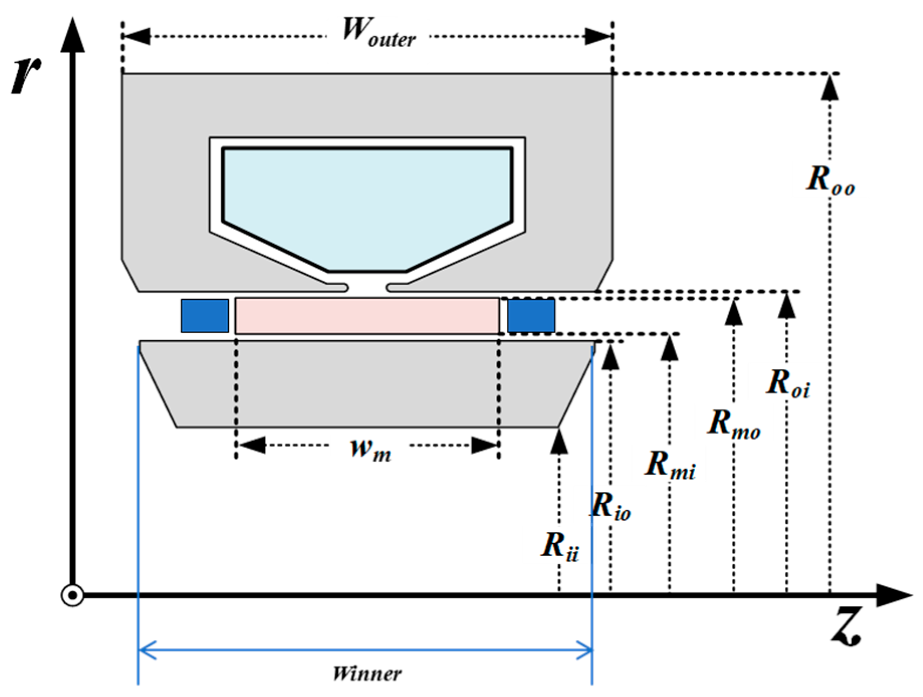
The essential dimensions used in the simulation of the model in Maxwell software are shown in Figure 3, which describe the length and width of all the parts of the generator in the center of the engine. These details are critical for design, because the 1 kW model is built according to these design criteria. All the numerical figures are in millimeters, as shown in

Table 3. The design dimensions of the 1 kW model.

Parameter	Value (mm)	Parameter	Value (mm)
Rii	52.5	Roo	116.5
Rio	67.5	Wouter	77
Rmi	69.5	Winner	67.7
Rmo	75.5	Wm1	33
Roi	76.5	Wm2	5

, and were derived from the engine’s center.

3.2. Cross-Sectionally Down-Scaling 1 kW Model from Full to Half Scale

Since the 1 kW model was scaled down to design the 50 W model, the approach aimed to decrease the 1 kW model step by step; initially, a LSF 0.9 model of the 1 kW model was created, then LSF 0.8, and so on until LSF 0.5. The rationale for not decreasing it further is mentioned in the preceding methodology: the stroke of 5.5 mm was reached with the LSF 0.5 model. Thus, the only adjustment needed is to adapt the generator to the engine. This section focuses on the design specifics of the 1 kW model and the outcomes of the gradual reduction in this model.

3.2.1. Analysis of the Cross-Sectionally Down-Scaled Models

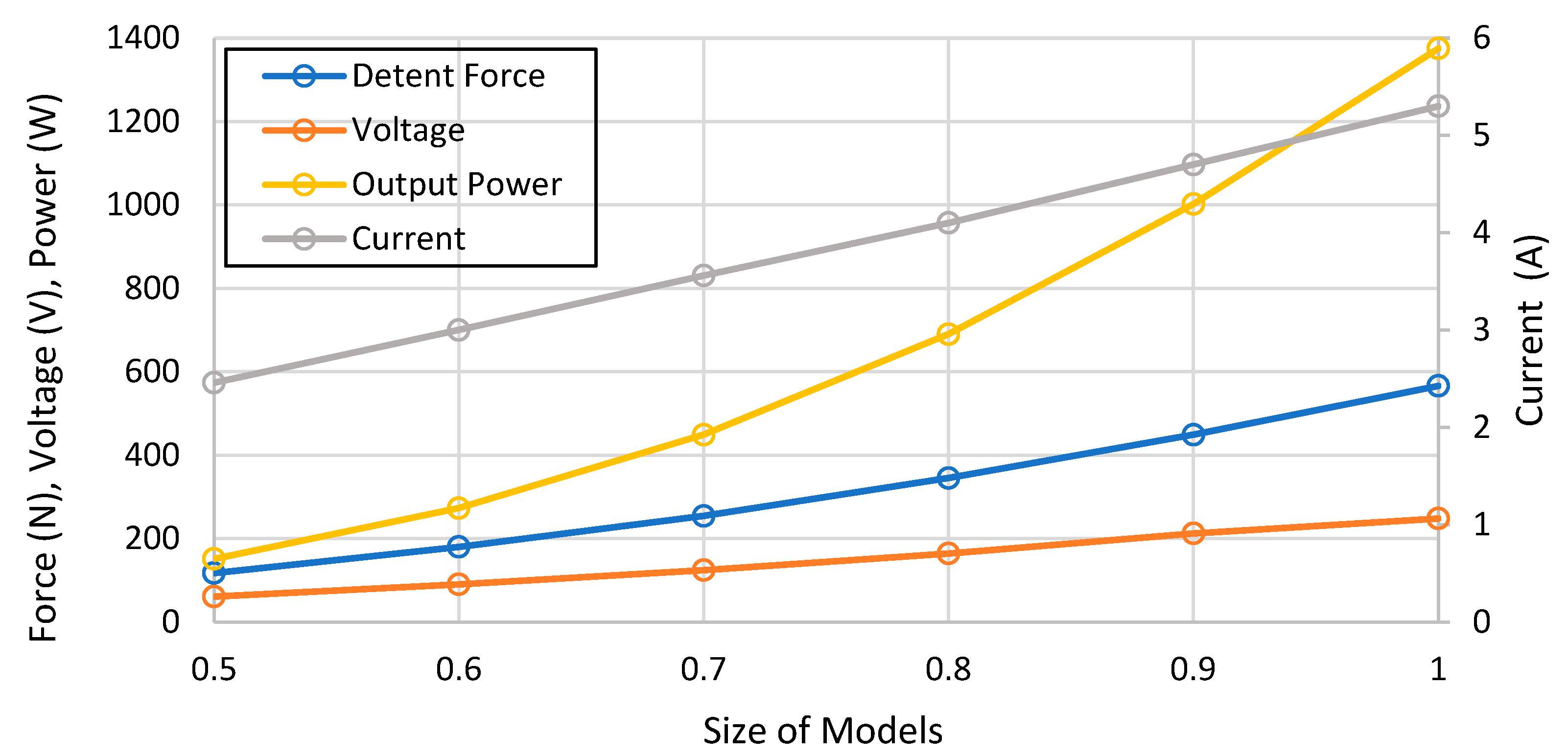
The 1 kW linear generator model was diminished in size sequentially, with the length scale factor (LSF) reduced from 1.0 to LSF 0.5. In this stepwise reduction, all of the design parameters of the 1 kW model were reduced to preserve consistency in reduction. The required stroke of 5.5 mm is needed for the engine, which is half the stroke of a 1 kW model. Therefore, FEM analysis was conducted to describe the trend of how power, voltage, current, and force change while stepwise reducing the 1 kW model shown in

Table 4. The results of stepwise-size reduced models; LSF (length scale factor) = 1 corresponds to the full-size 1 kW model. All other models are proportionally scaled versions.

LSF (Model)	Force (N)	Voltage (V)	Current (A)	Output Power (W)
1.0	566	248	5.3	1375
0.9	449	212	4.7	1002
0.8	345	164	4.1	690
0.7	254	124	3.56	449
0.6	180	90	3	273
0.5	117	61	2.46	151

.

It is evident in Table 4 that the LSF 0.5 model has an output power of 151 W, even though the stroke is 5.5 mm; however, our goal is to reach an output power of 50 W. This discrepancy arises because the distance from the generator’s inner core to the engine center in the LSF 0.5 model is 61 mm, which makes the overall size of the generator bigger (a radius of 84.5 mm). Such dimensions are incompatible with the engine, of which the total radius is limited to 90 mm. Therefore, to adapt the generator for integration with the Stirling engine, a radial reduction from the engine center is required. The details of this adjustment are discussed in a subsequent section of this paper.

The graph in Figure 4 indicates the combined result introduced in Table 4. On the x-axis, the model’s size is reduced from 0.5 to 1; 1 defines the actual design of the 1 kW model. On the left side of the y-axis, the output power, voltage, and force values are shown, whereas on the right side of the y-axis, the current values are shown. The trend in the graph shows that the force, voltage, and current have a linearly increasing trend, whereas the output power looks more like an exponentially rising graph.

3.2.2. No-Load Analysis of the Stepwise Reduction Models

The output electrical parameters were mentioned in the previous section in order to uncover the related results. The simulation steps/procedure were conducted, and the details of those steps and simulation conditions used in Maxwell software are discussed later. The term no load itself suggests that the simulation is performed without putting any load stress on the generator. Therefore, a no-load analysis of all the cross-sectionally reduced models in Maxwell software was performed.

The purpose of simulating a no-load analysis is to determine the stroke of the generator; the stroke of reduced models is estimated through no-load analysis as the zero-detent force length in the graph that shows the stroke length. The design goal is to achieve the detent force length of 5.5 mm, which will be the stroke of the 50 W model. Therefore, our analysis aims to reduce the model step by step in order to follow the zero detent trend illustrated in

Table 5. The no-load analysis of LSF models.

LSF (Model)	Detent Force (N)	Induced Voltage (V)	Zero Detent Force (mm)
1.0	265	88	±11
0.9	215	78	±10
0.8	200	66.5	±9
0.7	170	56.5	±8
0.6	140	47	±7
0.5	114	38	±5.5

.

The graph in Figure 5 illustrates how the value of the detent force and the induced voltage increase as the size increases from LSF 0.5 to the actual dimensions of the 1 kW model. Detent force is produced due to the magnetic interaction between the magnet and the cores when no current flows through the coil. The stroke (zero detent force distance) of the stepwise reduction model also shows how, in the 1 kW model, the 11 mm stroke was reduced to 5.5 mm.

3.2.3. Load Condition of the Models

In the no-load analysis, the stroke of the models was determined; therefore, the next simulation step, load analysis, was performed to determine the output electrical parameters of the model. Since load results can only be determined after applying load conditions, in this section, a calculation and further simulation were conducted to determine the load values for the stepwise reduction models. The aim of this section is to complete the simulation of the coil inductance.

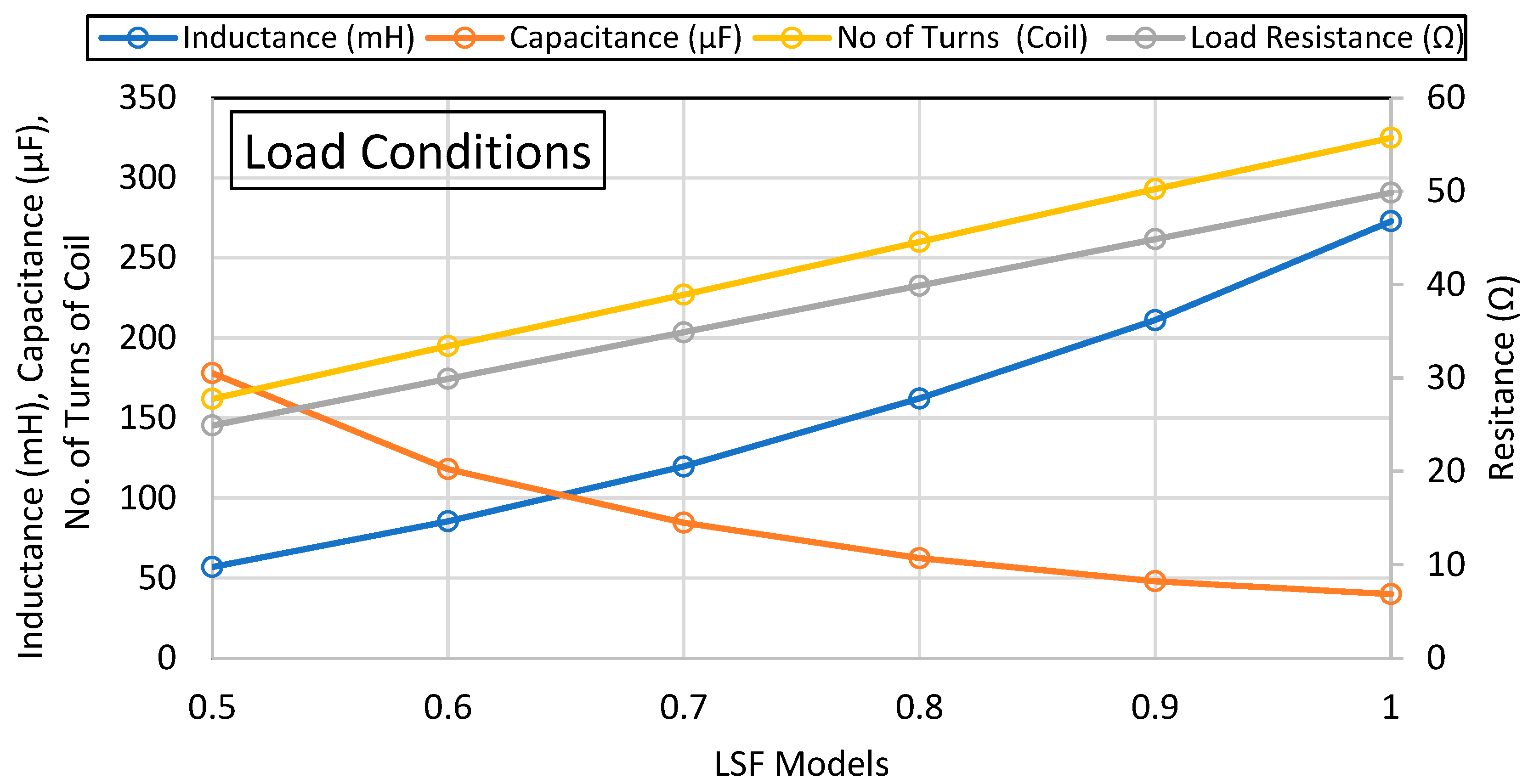
The solution type in Maxwell software from transient analysis was changed to a magnetostatic analysis. By completing the magnetostatic simulation of all the stepwise models, the inductance value of each model was determined. The inductance value of each model is different because every model has a different number of coil turns, and the coil area also differs; therefore, the inductance value increases with the increase in the size of the model. The capacitance for the stepwise reduction models was calculated using the formula of the resonance frequency and the inductance from the simulation. The operating frequency of the generator is 50 Hz; therefore, by applying the equation of the resonance frequency (2), the capacitance was calculated.

$$f={\displaystyle \frac{1}{2\pi \sqrt{\mathrm{L}\mathrm{C}}}}$$

(2)

As the specified load resistance was used in the simulation of the 1 kW model, the load resistance with the same parameter as the whole model was reduced for consistency in the stepwise model’s reduction.

Table 6. The load condition of the stepwise reduction models.

LSF (Model)	Inductance (mH)	Capacitance (µF)	Load Resistance (Ω)	No. of Turns (Coil)
1.0	273	40	49.85	325
0.9	211.10	48	44.86	293
0.8	162.19	62.4	39.88	260
0.7	119.72	84.6	34.89	227
0.6	85.44	118	29.91	195
0.5	56.92	178	24.925	162

shows the data produced in the simulation of the stepwise model. A total of 325 turns of the coil was selected in the design specification of the 1 kW model. To determine the rest of the stepwise reduction models, we can simply multiply that factor by the number of turns of the 1 kW model.

The No. of turns of the LSF 0.9 model was calculated by multiplying the No. of turns of the 1 kW model by 0.9—for example, 325 multiplied by 0.9 yields 293 turns. Figure 6 indicates the trend of the load condition of the stepwise models, showing a linearly incremental graph for resistance and coil turns, whereas inductance increases exponentially and capacitance decreases exponentially, verifying the inverse relation between capacitance and inductance.

3.2.4. Load Analysis of the Stepwise Reduction Models

The output parameters, like voltage, current, and power, are known from the simulation step of the load analysis using Maxwell software. This step is similar to the no-load analysis; however, specifically, this step is performed to determine the output power of the generator. Earlier load values or load circuit values were found and calculated; therefore, after setting the load condition and inserting the load circuit while winding the generator using Maxwell software, the load setup for the simulation was completed. Since the linear generator moves linearly, this specified linear movement is basically due to the magnet in the generator.

In the simulations, speed was assigned to the generator’s magnet to represent the linear motion characteristic of the system. The generator model was developed in 2D within Maxwell software, as 2D simulations are less computationally intensive than 3D simulations while yielding comparable accuracy. The magnet’s speed was applied linearly along the plane of the model. To represent the piston stroke, the magnet’s displacement was defined in terms of position, and a dedicated motion region was created within the model to specify its movement.

Firstly, the position for the magnet to move was set, as in the 1 kW model, and the movement position for the magnet in Maxwell software ranged from 25 mm to −25 mm, and the formula for setting the speed was

$$v\left(t\right)=\omega x_m\mathrm{c}\mathrm{o}\mathrm{s}\left(\omega t\right)$$

(3)

here, $x_m$ is the stroke amplitude, and $\omega$ is the angular frequency, with f being the operating frequency of the generator. Time is a variable term that changes with the analysis time. The speed for the LSF 0.9 model was 3.141 m/s.

The conditions for the load analysis were set, and the speed of the moving magnet was assigned; therefore, the analysis progressed, and the output values of the stepwise reduction models are shown in Table 4.

Figure 4 describes the voltage, current, and output power of the models. The output parameters decrease as the model’s dimensions decrease; similarly, the power reduces from 1375 W to 151 W.

In this analysis, a model with a stroke of 5.5 mm that fulfills the stroke requirement for the 50 W model was developed. However, the output value was far greater than our requirement. This was due to the distance from the inner and center of the generator being kept the same for all the stepwise reduce models.

3.3. Adjusting the LSF 0.5 Model in Radial Direction

The analysis of the 1 kW model produced a new model; the next step is to fit the model according to the symmetry of the Stirling engine, so in the next phase, we decreased the distance from the magnet to the center of the generator—in the LSF 0.5 model, it was 61 mm, whereas our requirement with a Stirling engine was 27 mm. By decreasing the center distance to 27 mm in the radial direction (Figure 7), the output power drastically decreased, because the generator size was reduced such that it reduced the power to below 50 W.

Furthermore, it was necessary to increase the air gap between the inner core and the magnet from 1 mm to 1.3 mm and the outer core air gap from 0.5 mm to 1 mm. These changes caused the output power to drop significantly to 37 W. To recover the target output of 50 W, several geometric parameters of the new model were adjusted, and the number of coil turns was increased from 162 to 220. With these modifications, the generator achieved approximately 50 W of output power while maintaining the stroke within the desired range of ±5 mm.

Maxwell’s design of the 50 W-2D model, after changing the geometry according to the engine, is shown in Figure 1b. In the 50 W model design, the outer core, inner core, coil, center, and spring magnet are defined, which completes and describes the geometry of the whole model.

3.3.1. Constraints in the 50 W Generator Design

The engine has an approximate size of 300 mm when combining all the parts of the engine, including the generator; therefore, there were strict size constraints when developing the generator.

As shown in the geometry of the engine in Figure 1a, the generator looks to fit within the 300 mm length of the engine. Therefore, the generator is 38 mm long, which makes it difficult to obtain the output power of 50 W. The second main constraint in developing the generator was the air gap between the magnet and the inner core. Initially, an air gap of 1 mm was selected; however, due to the engine’s design, a minimum air gap of 1.3 mm was required. This reduced the output power from 50 W to 37 W.

To further assess sensitivity to air gap variations, we conducted simulations with the magnet radial eccentricity ranging from 0 to 400 µm. The resulting side forces are summarized in

Table 7. The gap tolerance of the magnet.

Magnet Eccentricity (µm)	Force (N)
0	0.0236 N
20	2.86 N
50	7.0 N
100	14.09 N
200	28.3 N
400	58.18 N

:

These results show that air gap variations above 50 µm significantly affect electromagnetic stability, highlighting the importance of tight gap control in practical applications.

As discussed, the power dropped to 37 W after decreasing the center distance and the air gap. Therefore, to address this issue, a series of simulations was conducted. After multiple simulations, the coil turns were determined based on the available winding space and thermal/mechanical feasibility. Following consultation with the manufacturer, a 220-turn coil with AWG 19 copper wire was selected, along with a magnet thickness of 3.8 mm.

Compared to the geometry of the LSF 0.5 model, the magnet in the 50 W model is much thicker. Since there was a strict constraint on space in the 50 W model, even the inner core width was reduced from 5 mm to 4.5 mm, as there was no evident 0.5 mm effect in the output results of the generator. Furthermore, the results of the magnet’s thickness are particularly significant, as the magnet is the main source of power generation, making its effect particularly visible in the output. While changing the magnet thickness from 3 mm to 3.8 mm, the power ranged from 37 W to 47 W, such that at a magnet thickness of 3 mm, the output power was 37 W, and at a magnet thickness of 3.8 mm, the output power was 47 W. Later, load variation analysis was conducted to achieve exact 50 W power.

The simulation procedure was similar to the 1 kW model, so to overcome the design problems, no-load and load analysis simulations were carried out.

3.3.2. The 50 W Linear Generator No-Load Analysis

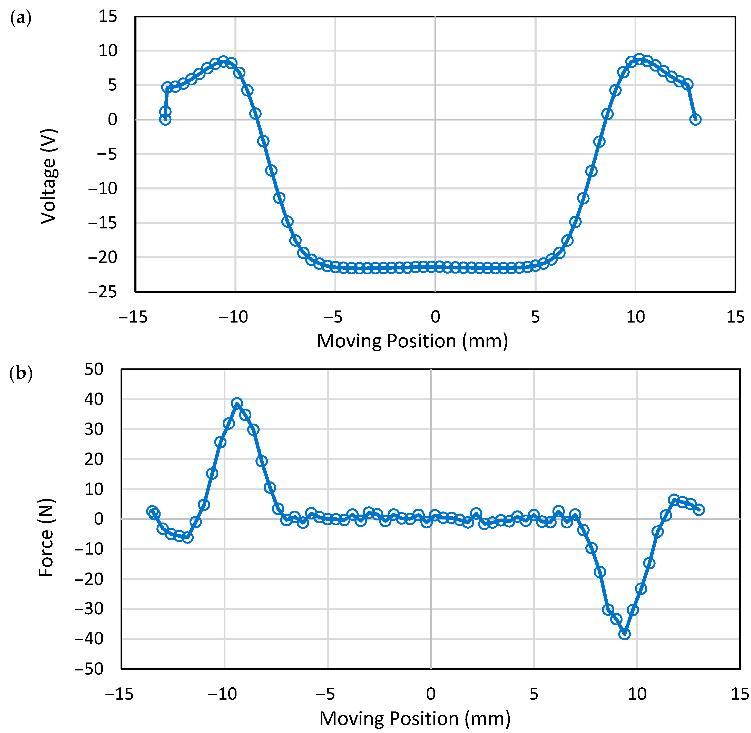
After adjusting the design dimensions to match the engine, a no-load analysis was conducted to verify the detent force distance and confirm the stroke of the 50 W model. The target detent force length of 5.5 mm, corresponding to the stroke of the 50 W model, was successfully achieved. The no-load analysis results, compared with those of the LSF 0.5 version of the 1 kW model, are shown in

Table 8. The no-load analysis of the 50 W generator model.

Parameter	LSF 0.5 Model	50 W Model
Distance of Magnet from the Center (mm)	61	27
Detent Force Amplitude (N)	114	39.5
Voltage Amplitude (V)	38	21.21
Zero Detent Force Distance (mm)	±5.5	±6

.

The stroke of the new model was greater than the LSF 0.5 model, since a slight tolerance was considered; the model was designed in a way to have a zero detent force distance of 6 mm to −6 mm. The parameter values of the LSF 0.5 model were far greater than the 50 W model; the reason for this is the same reason mentioned in Table 8. The magnet distance from the center is far greater than in the 50 W model, which increases the size of the LSF 0.5 model and increases its power. Figure 8a shows the induced voltage at a mover constant speed of 1 m/s. The force is constant in the stroke region. The detent force according to the mover position was not generated in the stroke region, as shown in Figure 8b.

3.3.3. Load Analysis of 50 W Linear Generator

In the no-load analysis, the stroke was within the target range; therefore, the next step was to conduct a load analysis. To begin the load analysis, the load condition must be determined. In Maxwell software, the solution type is switched from transient analysis to magnetostatics to calculate the inductance of the coil in the model. Subsequently, magnetostatic simulations were performed for the model to determine its inductance. The inductance found using Maxwell software for the 50 W model was 44.69 mH, and by using the resonance frequency formula, we calculated the capacitance to be 226 µF. A total of 220 turns with a coil diameter of 0.9 mm was maintained.

After setting the load condition and inserting the load circuit into the generator winding in Maxwell software, the next setup is to allocate the speed to the generator’s magnet. Given that the generator is linear and the Maxwell design is in 2D, the speed is linearly assigned to the model’s plane. Initially, the position for the magnet’s movement is set; for example, in the 50 W model, the magnet’s movement position in Maxwell software is set from 13.5 mm to −13.5 mm. The calculation used for setting the speed is as follows:

$$v=x_{m}2\pi f\mathrm{c}\mathrm{o}\mathrm{s}\left(2\pi ft\right)=1.727\mathrm{c}\mathrm{o}\mathrm{s}\left(100\pi t\right) \mathrm{m}/\mathrm{s}$$

(4)

By setting the speed and load condition, simulation results of current and voltage were determined.

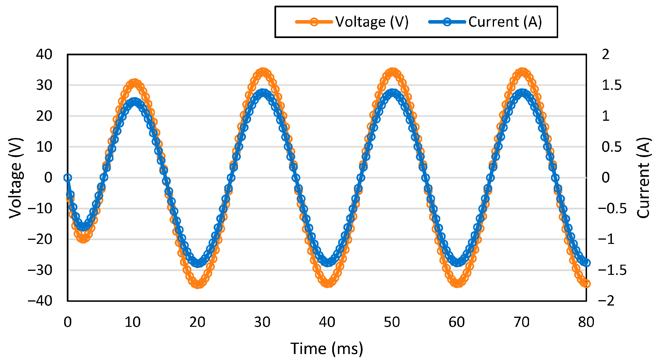
In the load analysis, the output voltage was 34.6 V (rms value), as shown in Figure 9, and the output current was 1.37 A (rms value), as shown in

Table 9. The load analysis result of the 50 W generator model compared with the LSF 0.5 model.

Parameter	LSF 0.5 Model	50 W Model
Distance of Magnet from the Center (mm)	61	27
Detent Force Amplitude (N)	117	43
Voltage Amplitude (V)	61	34.6
Current Amplitude (A)	2.46	1.37
Output Power Amplitude (W)	151	47.5
Zero Detent Force Distance (mm)	±5.5	±6

. The output power, when using a load resistance of 24.9 Ω, was 47.5 W.

Table 9 describes the force, voltage, current, and output power of the models. The values of voltage and current are within the target range, but the output power graph shown in Figure 10 is not exactly 50 W; therefore, load variation was performed, and by changing the load resistance, the output power of 50 W was achieved. Therefore, when continuing our research, further simulation of the variation in load resistance was carried out.

3.4. Analysis of Varying the Load for the Final Design

The above FEM analysis yielded the output power of 47 W; however, the design goal is 50 W. To achieve that power, load variation analysis on the 50 W model was performed. By applying load variation, the effect of load resistance and capacitance on the design becomes apparent. Therefore, first, the resistance is changed, and the values at which the output power is 50 W are extracted by repeating the load analysis step, such that while adding the circuit in the winding and changing its resistance, the rest of the steps were the same.

3.4.1. Varying the Resistance

By changing the resistance to 23 Ω, as shown in

Table 10. Load variation, i.e., changing the resistance of the 50 W generator model.

Load R (Ohm)	Output Power (W)	Output Voltage (V)	Output Current (A)	Efficiency (%)
26	45.75	34.49	1.32	89.5
24.9	47.5	34.37	1.37	90.47
24	49.06	34.33	1.42	89.46
23	50.89	34.23	1.48	89.40
22	52.85	34.13	1.54	89.32
21	54.99	33.87	1.61	89.26
20	57.28	33.72	1.68	90.0

, the output power of 50.5 W was obtained. Therefore, the output power was adjusted in the simulation by varying the load resistance to achieve exactly 50 W RMS. Although the coil turn counts were not explicitly varied, the selected coil design (220 turns of AWG 19 wire) was based on the available slot area and validated through manufacturer consultation.

As shown in Table 10, the output power was analyzed at 50 W, and the efficiency of the model was approx. 90%, which also fulfills the requirement for modeling of this design. However, to evaluate robustness against manufacturing variability, simulations were conducted with magnet eccentricities ranging from 20 µm to 400 µm, as shown in Table 8. The results showed that the generator maintained output power within ±5% deviation, demonstrating good tolerance to small physical misalignments.

While magnet grade variation and coil turn deviations were not directly simulated, the current design includes sufficient design margins in magnetic loading and winding space to accommodate minor manufacturing tolerances.

As shown in the table, the current increased as the resistance was decreased, and the voltage decreased with a decrease in the resistance, such that it was directly proportional to resistance. The trend is evidently based on Ohm’s law [28].

The impact of varying the resistance is much more prominent when moving below or above 23 ohms. Following efficiency, it decreases with a decrease in resistance, and vice versa.

3.4.2. Varying the Capacitance

The winding and manufacturing attributes of an SPLPMG (Single-Phase Linear Permanent Magnet Generator) result in a high inductance component. Therefore, the resonant frequency must be considered when implementing the tuning capacitors to maximize the output power. The equivalent circuit for the SPLPMG is mentioned in Figure 11 [21].

The electrical equivalent equation based on the circuit is given by the following:

1.

The equation for the current dynamics [29]:

$$R_a+L_a{\displaystyle \frac{di}{dt}}+{\displaystyle \frac{1}{C}}\int idt=E_0-V_t$$

(5)

where R_a is the winding resistance, L_a is the inductance, C is the tuning capacitance, E₀ is the induced voltage, and V_t is the terminal voltage

2.

The load voltage expression given by

$$V_t=E_0\sqrt{{\displaystyle \frac{R_L}{{\left(R_a+R_L\right)}^2+{\left(X_a-X_C\right)}^2}}}$$

(6)

here, R_L is the load resistance, $X_a$ is the inductive reactance of winding, and $X_C$ is the capacitive reactance of the tuning capacitor.

The tuning capacitance was selected to cater to the winding inductance. Therefore, when $\left(X_a-X_C\right)=0$ the load voltage becomes maximum. Hence, by applying the different capacitance values, the effect of the capacitor on the output parameters of the linear generator was attained, as mentioned in

Table 11. Variation in the capacitance of the 50 W generator model.

Load R (Ohm)	Capacitive Load (µF)	Output Power (W)	Output Voltage (V)	Output Current (A)	Efficiency (%)
24.9	230	47.51	34.41	1.37	89.44
	226	47.5	34.37	1.37	90.47
	210	47.2	34.23	1.371	90.59
	200	46.83	34.06	1.36	89.53
	180	45.83	33.47	1.33	90.49
	150	42.85	32.67	1.30	88.62

.

At 226 µF of impedance, $\left(X_a-X_C\right)=0$; therefore, at this capacitance, the power is maximum.

The equivalent load circuit combined with a linear generator’s winding during load analysis using Maxwell software is shown in Figure 12. An inductor, a load resistor, and a tuning capacitor comprise the circuit’s winding. This setup aids in simulating how the generator will behave under various load scenarios. In order to maximize power transmission from the generator winding to the load, the tuning capacitance is adjusted to match the reactive power and guarantee resonance within the circuit.

The data values acquired by adjusting the tuning capacitance in the Maxwell simulation are displayed in Table 10 and Table 11. Along with the output voltage and the current flowing through the winding, the values also contain measurements of the voltage across the resistor and capacitor. By affecting the impedance matching and overall power transfer efficiency, these data points provide clarity on the generator’s performance characteristics as the tuning capacitance is changed.

3.4.3. Loss Analysis of 50 W Linear Generator

In a further analysis of the 50 W model, loss analysis was conducted, which includes the loss in all the parts of the linear generator. The target efficiency of approximately 90% was derived from the simulation results, which account for copper losses (I²R), core losses (including hysteresis and eddy currents), and magnet eddy losses (solid losses) [30]. However, the simulations do not include certain practical losses, such as connector resistance, external wiring losses, contact resistance, and thermal derating effects.

There was no option for loss analysis of each part of the generator in MAXWELL software; therefore, referring to the newer version of FEM analysis, Ansys Electronics was used to conduct the loss analysis. The reason for using Ansys Electronics is that it utilizes the same software setup. As for the simulation, the analysis steps are the same. However, for the loss analysis, specific options must be marked before the simulation.

Table 12. Loss analysis of the 50 W generator model.

Part Name	Core Loss (W)	Eddy Current Loss (W)	Excess Loss (W)	Hysteresis Loss (W)	Per Winding Strande Loss (W)	Solid Loss (W)
Outer core	0.3195	0.0528	0.0387	0.229	-	-
Inner core	0.095	0.01865	0.01155	0.065	-	-
Coil	-	-	-	-	1.995	-
Center magnet	-	-	-	-	-	0.7265
Spring magnet 1	-	-	-	-	-	0.125
Spring magnet 2	-	-	-	-	-	0.125
Total Loss	0.4097	0.073	0.0498	0.29035	1.995	0.918

describes the loss of the parts of the generator. The maximum loss was calculated in the winding of the generator, namely, the stranded loss. Based on typical system-level experience, these additional losses are expected to reduce overall efficiency by approximately 5% [31]. Therefore, the practical efficiency of the generator is estimated to be closer to 85% under real operating conditions.

The total loss by the model is about 3.7 W, and the losses are defined by how they are computed in Ansys software. The separation of core, eddy, hysteresis, and strand losses was performed using the post-processing features in ANSYS Electronics, as the standard MAXWELL solver does not provide a part-wise loss breakdown directly. The methodology used is as follows:

• Core losses were computed using the material’s B–H curve and Steinmetz-based models embedded in ANSYS.
• Hysteresis losses were implicitly included as part of the total core losses, according to the loss modeling settings.
• Eddy current (solid) losses were extracted by enabling the “Eddy Effect” setting on the magnets.
• Stranded (proximity) losses were calculated by integrating the induced current density over the copper conductor volumes.

To validate the separation, we compared the total loss obtained from the combined simulation with the sum of individual components to ensure consistency. Additionally, the trend of each loss component under different excitation frequencies and loading conditions was examined for physical plausibility and correlation with expected behavior.

3.4.4. Phasor Diagram Analysis

The Phasor diagram was generated in MATLAB R2024a software. The amplitude and angle of the voltage and current were extracted from graphs generated using MAXWELL software, with additional parameters calculated as required. The detailed calculation process is mentioned in a later section.

The data in

Table 13. The phasor values of the parameters sourced from the Maxwell graphs.

Vector	Magnitude (V)	Phase (Angle)
Induced Voltage	56	~144
Capacitor Voltage	27.4	−90
Resistance Voltage	48.62	0
Current (Reference)	1.95	0

were sourced from the graphs of the 50 W model using Maxwell software. Following the load analysis, load conditions were calculated. Using these load values, a combined equivalent circuit was created in the Maxwell circuit editor for the 50 W model. The circuit was then inserted more accurately into the model during coil winding in Maxwell software, as shown in Figure 12.

The phasor diagram, referring to the vector values generated by Maxwell software, is mentioned in Figure 13.

The voltages and current of the circuit are depicted in Figure 13 through a phasor diagram, illustrating their magnitudes and phase angles obtained from Maxwell software simulations. The diagram illustrates the correlation between the voltages across the resistor (red), capacitor (blue), inductor (cyan), terminal voltage (black), and the induced voltage during winding (magenta). By displaying the phase shifts between these components, the phasor angles provide crucial insights into the dynamic behavior of the generator during operation. The phasor diagram emphasizes the impact of the tuning capacitor on the phase relationships and the overall resonance of the system, which is vital for optimizing the power output of the linear generator.

4. Comparison to SAGE Predictions

The previous analysis found the output power of the generator to be 50 W; however, the linear generator is a subsystem of the Stirling engine. Therefore, to complete the assembly of the engine, this linear generator should be connected with the engine and simulated in a single software environment. To accomplish this, SAGE software was used which allows us to connect the generator and engine under one software program and conduct a complete simulation of the engine. The generator cannot be connected with the engine in Maxwell software, as Maxwell only has electrical simulation results, and it cannot solve the mechanical components of the engine.

In this study, mechanical resonance and structural vibration coupling between the generator and the Stirling engine were not explicitly modeled. The use of SAGE software focused solely on simulating the electromechanical characteristics of the linear generator as a subsystem without incorporating detailed dynamics of the entire engine–generator assembly.

It was noted that vibration and mechanical resonance can influence long-term reliability, especially under harsh or variable conditions, such as those in space applications. This aspect is recognized as a limitation of the current study and is intended to be addressed in future work through integrated dynamic modeling or experimental validation.

4.1. SAGE Model of Linear Generator

The 50 W models in Maxwell software comprise different parts, including the geometry of the generator. In the same way, SAGE also includes the parts of a generator, but rather than using 2D symmetry, SAGE has 1D symmetry, and it uses a block that represents backend solving, which performs the analysis by passing the required values. The results computed by SAGE utilize the numerical solvers technique to solve the complex differential equations that govern thermodynamics and mechanical dynamics. These solvers typically use iteration to improve their solutions until the system achieves a stable point or the desired level of accuracy.

Figure 14 is a representation of an SAGE electromechanical (E-M) model, and the key components include the following:

• Voltage reference.
• Load resistor.
• Capacitor.
• Moving magnet motor.
• Fixed iron reference and moving magnet driver.
• Spring.

The block of greatest concern in this paper is the moving magnet motor part of the EM model, as the main parts of the generator are placed under this block, forming a sub-block part of the model shown in Figure 15.

Moving on, there are necessary parts, like the outer core, inner core, magnet, and coil of the generator under the moving magnet motor block. We took the liberty of passing the values to these sub-blocks so that SAGE can compute the results.

More importantly, SAGE analyzes based on 1-dimensional symmetry. The model that SAGE simulates for analysis is significantly simpler than the actual model. One of the noticeable changes is that the coil design in the Maxwell software is more like the pentagon shape to increase the efficiency of the generator, but SAGE does not account for such geometric detail when solving. Therefore, the inadequacy in creating the particular shape in SAGE software causes the model to deviate from the actual one in Maxwell software. Such a difference is notable in Figure 16, which shows that the SAGE model is more likely to be considered in SAGE software versus the actual model created using Maxwell software.

4.2. SAGE Model Simulations

As the SAGE model cannot be compared with the current 50 W model because of the different design shape, it was necessary to design a new model similar to the SAGE model. This new model, referred to as the SAGE Maxwell Model and shown in Figure 17, replicates the SAGE E-M model presented in Figure 16. The same no-load and load analysis procedures used for the 50 W model were applied to the SAGE Maxwell Model to enable a direct comparison of the results from both software tools.

4.2.1. SAGE Maxwell Model Results

In this section, the results from the load analysis are discussed, as the main goal is to compare the output power results from both software programs. Therefore, in the analysis of the SAGE Maxwell Model, the output power achieved was 45 W.

Table 14. SAGE Maxwell model results.

Parameter	SAGE Maxwell Model
Force Amplitude (N)	39.59
Voltage Amplitude (V)	33.23
Current Amplitude (A)	1.33
Output Power Amplitude (W)	45
Zero Detent Force Distance (mm)	±5

depicts the results, the numerical values, of the SAGE Maxwell model, including power, voltage, and current. The values that are mentioned in Table 14 are the rms values.

4.2.2. SAGE Results

The parameters and dimensions used for the analysis in SAGE were assigned according to the values mentioned in Table 14 for the SAGE–Maxwell model. While setting the values, the objective was to ensure consistency with the 50 W model.

The SAGE analysis result yielded an output power of approx. 38 W, as shown in

Table 15. A comparison of the 50 W generator model, SAGE Maxwell model, and SAGE model.

Parameter		50 W Generator	SAGE Maxwell Model	SAGE Model
Power (W)		47.5	45	37.79
Voltage (V)		34.6	33.37	30.6
Current (A)		1.37	1.33	1.23
Inductance (mH)	Load Condition	44.74	65.8	66.1
Capacitance (µF)		226	154	154
Resistance (Ω)		24.925

.

Other than the 50 W model, there were two more models, namely the SAGE model and the SAGE Maxwell model. The main goal was to compare the results; therefore, Table 15 shows a comparison of the electrical parameters of these models.

Since the values are not the same in the SAGE–Maxwell model and SAGE model, even while having the same design symmetry, a loss analysis was conducted for both models.

4.2.3. Loss Analysis

The Sage loss analysis results show that the total loss in the SAGE model is approximately 2.5 W, and the total loss of the SAGE Maxwell model is approximately 4 W rms.

The loss comparison between two models shows the difference in the losses by parts in

Table 16. Loss comparison.

Losses (W)	SAGE Maxwell Model	SAGE Model
Coil	2.178	2.22
Inner core (Eddy)	0.018	0.0314
Outer Core (Eddy)	0.059	0.066
Inner core (Hysteresis)	0.0615	0.16
Outer Core (Hysteresis)	0.266	0.12
Magnet	0.8835	0.069

.

As shown in Table 16, the SAGE model loss is around ¾ times less compared to the SAGE Maxwell model. The particular reason is that SAGE did not consider the losses as much as Maxwell did in the FEM analysis, and the analysis of the discrepancy in the output power and the losses is discussed in the next section.

4.3. Analysis of the Discrepancies

Since there was a difference in the power, we conducted a loss comparison of both models, but this still did not provide the reason for the difference in the power. Thus, we checked the material properties used in the SAGE Model with the material used in the SAGE Maxwell Model. The material used for the cores of the SAGE Maxwell Model was 35PN230, whereas the material used in the SAGE model was silicon steel; therefore, for consistency, the SAGE core material was changed to 35PN230, but still, there was no evident change in the output power.

Hence, this analysis concluded that there are two possible reasons for the discrepancy.

i

Different Modeling Assumptions

(a)

Maxwell (Electromagnetic Analysis):

Maxwell is an electromagnetic field simulation tool that heavily relies on solving Maxwell’s equations using the Finite Element Method (FEM).

Maxwell calculates the behavior of the electromagnetic fields within the generator based on the geometry and material properties. The FEM divides the geometry into small elements, and the fields are calculated at discrete points. The localized nature of these calculations means that Maxwell can accurately simulate variations in the magnetic flux, eddy currents, and core losses, which directly affect output power [32].

• (b)

  SAGE (System-Level Analysis):

SAGE, a system-level simulation tool, uses lumped parameter models to simulate the electrical, mechanical, and thermodynamic behavior of systems. Regarding the reason for the discrepancy, lumped models simplify the generator into a set of resistances, inductances, and capacitances that represent the overall behavior of the system rather than detailed local interactions. For instance, SAGE might apply Kirchhoff’s laws to simplified circuit models.

These simplifications may omit localized electromagnetic effects (such as skin effect and proximity effect in conductors) and may result in lower predicted power output because of the averaging inherent in these models [33].

This method of solving in SAGE is known as the Finite Difference Method (FDM). This method involves discretizing the governing differential equations into a grid of points and solving the system iteratively. It is typically simpler and faster for solving problems in structured grids.

ii

Different Solver Approaches

(a)

Maxwell’s FEM Solver:

Maxwell uses FEM to solve for electromagnetic fields by discretizing the domain into finite elements. The fundamental equation solved in this case is the Helmholtz equation [34] derived from Maxwell’s equations in the frequency domain:

$$\nabla \times \left({\displaystyle \frac{1}{\mu }}\nabla \times E\right)-{\omega }^2ϵE=-j\omega J$$

(7)

where E is the electric field, μ is the permeability, ϵ is the permittivity, J is the current density, and ω is the angular frequency. This allows Maxwell to account for the spatial distribution of currents and fields with high precision.

The FEM method breaks the domain into a mesh of small elements and uses variational methods (such as Galerkin’s method) to approximate the solution. The higher the mesh density, the more accurate the solution, but at the cost of computational time. Maxwell can accurately model transient and dynamic effects, such as eddy currents and non-linear magnetic saturation, which can lead to more precise output power calculations [35].

• (b)

  SAGE’s Simplified Solver:

SAGE, instead of FEM, uses simplified models, often based on analytical equations or semi-empirical relations. For example, it may solve the generator’s electrical performance using the equivalent circuit method:

$$V=IR+L{\displaystyle \frac{dI}{dt}}$$

(8)

This method approximates the inductance and resistance of the generator in a time-dependent manner but does not consider spatial variations in the magnetic field. The simplification can result in an underestimation of the output power since localized phenomena like leakage flux and fringing effects are often averaged out or ignored.

The exact equation or a particular method about how SAGE computes results is not mentioned in the literature. While searching thoroughly through the SAGE manual and also looking through previous papers on the SAGE simulation, there was little information about which kind of equation or what solving technique SAGE is based on to compute the E-M model results. Therefore, the discrepancy between both software’s result may be due to both using different solving techniques and the model assumptions used in the software being quite different.

5. Conclusions

The research goal of a 50 W model with 90% efficiency was achieved in this study using the base design of an already developed 1 kW model. Researchers working on linear generators for RSC, particularly low-power generators, will find this study’s contribution helpful. Nuclear power technologies can be assessed on the lunar surface and are now being developed for possible usage in space applications. With these technologies, heat from decaying isotope fuels might be transformed into useful electricity for spacecraft operations using such linear generators, because they consume less fuel (heat) to provide the necessary amount of system power. As a result, isotope fuel storage, waste heat, and radiation emissions may be decreased.

Free-piston Stirling converters are a key technology in nuclear power systems designed to supply electricity for space science missions. They are particularly well suited for environments where solar energy is not viable, such as dark, dusty, or remote locations. In these systems, heat from the radioactive decay of isotopes is converted into electrical power through a high-efficiency linear alternator, enabling a wide range of power outputs. Their lightweight design, versatility, and high efficiency make them adaptable to multiple applications, including systems comparable to the engines. Their compact size makes them suitable for powering humanoid robots, radioisotope power sources, space exploration, and more. Future work on the model can focus on compacting the size of the model, reducing the weight of the generator in the selection of the material, or resizing the core for optimal use. The limitations of the current study will be addressed in future work through integrated dynamic modeling or experimental validation. Moreover, these models can be used to develop generators with different power outputs, as this model produced results and parameters that can affect the output power, and by manipulating those parameters, a new model could be achieved.

References

1. Sunpower/Ametek. About Sunpower, Milestones. Available online: https://www.sunpowerinc.com/about-sunpower/milestones (accessed on 13 July 2025).
2. Gary, W.J.; Neill, L. Advanced 35 W Free-Piston Stirling Engine for Space Power Applications. AIP Conf. Proc. 2003, 654, 662–667. [Google Scholar] [CrossRef]
3. Gary, W.J.; Neill, L. Development of the Sunpower 35 We Free-Piston Stirling Convertor. AIP Conf. Proc. 2005, 746, 682–687. [Google Scholar] [CrossRef]
4. Wilson, S. High Efficiency Stirling Power Conversion Technologies for Radioisotope and Fission Nuclear Power Systems. In Proceedings of the Outer Planets Assessment Group (OPAG), Boulder, CO, USA, 27–29 November 2023. [Google Scholar]
5. NASA SPINOFF. Powering the Future. 2002. Available online: https://spinoff.nasa.gov/spinoff2002/er_9.html (accessed on 13 July 2025).
6. Oriti, S.M.; Wilson, S. Dynamic Power Convertor Development for Radioisotope Power Systems at NASA Glenn Research Center; NTRS, NASA Glenn Research Center: Cleveland, OH, USA, 2018.
7. Oriti, S.M.; Schreiber, J.G. Design and Fabrication of a Stirling Thermal Vacuum Test; NTRS, NASA Glenn Research Center: Cleveland, OH, USA, 2004.
8. Mason, L.S.; Schreiber, J.G. A Historical Review of Brayton and Stirling Power Conversion Technologies for Space Applications; NTRS, NASA Glenn Research Center: Cleveland, OH, USA, 2007.
9. Gibson, M.A.; Poston, D.I.; McClure, P.; Godfroy, T.J.; Briggs, M.H.; Sanzi, J.L. Kilopower Reactor Using Stirling TechnologY (KRUSTY) Nuclear Ground Test Results and Lessons Learned; NTRS, NASA Glenn Research Center: Cleveland, OH, USA, 2018.
10. Thombare, D.; Verma, S. Technological development in the Stirling cycle engines. Renew. Sustain. Energy Rev. 2006, 12, 1–38. [Google Scholar] [CrossRef]
11. Wikipedia Contributors. Faraday’s Law of Induction. Wikipedia. 20 January 2025. Available online: https://en.wikipedia.org/wiki/Faraday%27s_law_of_induction (accessed on 13 July 2025).
12. Boldea, I. Linear single-phase PM brushless motor. In Linear Electric Machines, Drives, and MAGLEVs Handbook, 2nd ed.; CRC Press: Boca Raton, FL, USA, 2023; pp. 489–502. [Google Scholar] [CrossRef]
13. Jia, Z.; Wang, R.; Hu, J.; Zhang, L.; Wu, Z.; Chen, Y.; Luo, E. Study on the coupling between engine and alternator in a free-piston Stirling generator. Appl. Therm. Eng. 2022, 217, 119222. [Google Scholar] [CrossRef]
14. Chi, C.; Li, R.; Mou, J.; Lin, M.; Jiao, K.; Yang, M.; Liu, H.; Hong, G. Theoretical and experimental study of free piston Stirling generator for high cold end temperatures. Energy 2024, 289, 129841. [Google Scholar] [CrossRef]
15. Lee, C. Turbine-Compound Free-Piston Linear Alternator Engine. CORE. 2014. Available online: https://core.ac.uk/outputs/20392042/ (accessed on 13 July 2025).
16. Meymian, N.Z. Design and Optimization of Dynamic System for a One-kW Free Piston Linear Engine Alternator-GENSETS Program. Ph.D. Thesis, West Virginia University, Morgantown, WV, USA, 2018; pp. 154–196. Available online: https://researchrepository.wvu.edu/etd/7927/ (accessed on 13 July 2025).
17. Chen, J.; Zhu, R.; Chen, Z.; Li, J.; Jin, J.; Chen, J.; Li, Y.; Zhang, Q.; Liu, S. Influence of Temperature on Magnetic Properties of Silicon Steel Lamination. AIP Adv. 2017, 7, 056222. [Google Scholar] [CrossRef]
18. Xue, S.; Chu, W.Q.; Zhu, Z.Q.; Peng, J.; Guo, S.; Feng, J. Iron Loss Calculation Considering Temperature Influence in Non-Oriented Steel Laminations. IET Sci. Meas. Technol. 2016, 10, 846–854. [Google Scholar] [CrossRef]
19. Mainrich Magnet Co., Ltd. High Temperature Neodymium Magnets—Grades and Operating Limits. Available online: https://mainrichmagnets.com/high-temperature-neodymium-magnets (accessed on 13 July 2025).
20. Kähkönen, O.-P.; Mäkinen, S.; Talvitie, M.; Manninen, M. Radiation damage in Nd-Fe-B magnets: Temperature and shape effects. J. Phys. Condens. Matter 1992, 4, 1007–1014. [Google Scholar] [CrossRef]
21. Lee, K.; Lee, S.; Park, J.; Choi, J.; Sim, K. Design and experimental analysis of a 3 kW Single-Phase linear permanent magnet generator for Stirling engines. IEEE Trans. Magn. 2018, 54, 1–5. [Google Scholar] [CrossRef]
22. Hadžiselimović, M.; Srpčič, G.; Brinovar, I.; Praunseis, Z.; Seme, S.; Štumberger, B. A novel concept of linear oscillatory synchronous generator designed for a Stirling engine. Energy 2019, 180, 19–27. [Google Scholar] [CrossRef]
23. Kim, J.; Choi, J.; Lee, K.; Lee, S. Design and analysis of linear oscillatory single-phase permanent magnet generator for free-piston Stirling engine systems. AIP Adv. 2017, 7, 056667. [Google Scholar] [CrossRef]
24. Oros, T.S.; Vadan, I.; Pop, R.; Brad, C. Linear Generator for a Free Piston Stirling Engine. J. Electr. Electron. Eng. 2014, 111, 111–112. [Google Scholar]
25. Metscher, J.; Lewandowski, E.J. Development and validation of an advanced stirling convertor model and simulation tool. In Proceedings of the 12th International Energy Conversion Engineering Conference, Cleveland, OH, USA, 28–30 July 2014. [Google Scholar] [CrossRef]
26. Li, Z.; Zhou, L.; Gong, Y.; Shen, F.; Peng, Y.; Wu, H. Axial Flux Electromagnetic Energy Harvester Driven by a Stirling Engine for Waste Heat Recovery. Energies 2025, 18, 1620. [Google Scholar] [CrossRef]
27. Yang, D.M. Review of Controllers for Low-Power Free-Piston Stirling Convertors. NASA Technical Memorandum NASA/TM-20220000637, July 2022. Available online: https://ntrs.nasa.gov/citations/20220000637 (accessed on 13 July 2025).
28. The Editors of Encyclopaedia Britannica. Ohm’s Law | Physics, Electric Current, Voltage. Encyclopedia Britannica. 21 December 2024. Available online: https://www.britannica.com/science/Ohms-law (accessed on 13 July 2025).
29. Dorf, R.C. Dynamic Equations and Their Solutions for Simple Circuits. 2010. Available online: https://introcontrol.mit.edu/_static/fall24/extras/siebert1.pdf (accessed on 13 July 2025).
30. Hu, Y.; Xu, Z.; Yang, L.; Liu, L. Electromagnetic loss analysis of a linear motor system designed for a free-piston engine generator. Electronics 2020, 9, 621. [Google Scholar] [CrossRef]
31. Arslan, S. Linear generator design for concentrating solar power. IET Renew. Power Gener. 2023, 17, 3712–3723. [Google Scholar] [CrossRef]
32. Wikipedia Contributors. Electromagnetic Wave Equation. Wikipedia. 7 December 2024. Available online: https://en.wikipedia.org/wiki/Electromagnetic_wave_equation (accessed on 13 July 2025).
33. Dyson, R.W.; Wilson, S.D.; Tew, R.C. Review of Computational Stirling Analysis Methods. In NASA/TM (Report No. 2004-213300). National Aeronautics and Space Administration. 2004. Available online: https://ntrs.nasa.gov/api/citations/20040171934/downloads/20040171934.pdf (accessed on 13 July 2025).
34. Ploier, A.; Kepler, J. From Maxwell to Helmholtz (By Johannes Kepler Universität Linz & Institut für Numerische Mathematik). 2017. Available online: https://numa.jku.at/media/filer_public/de/8c/de8c6589-ba58-4a41-8e09-d43154a06f33/bachelor-ploier.pdf (accessed on 13 July 2025).
35. Bastos, J.P.A.; Sadowski, N. Electromagnetic Modeling by Finite Element Methods; CRC Press eBooks: Boca Raton, FL, USA, 2003. [Google Scholar] [CrossRef]
Figure 1. (a) Position of the generator in the engine; (b) the linear generator.
Energies 18 04731 g001
Figure 2. An overview of the 1 kW model.
Energies 18 04731 g002
Figure 3. The design dimensions.
Energies 18 04731 g003
Figure 4. A comparison of length scale factor models.
Energies 18 04731 g004
Figure 5. The no-load comparison analysis of the LSF models.
Energies 18 04731 g005
Figure 6. A comparison of the load conditions of LSF models.
Energies 18 04731 g006
Figure 7. The distance of the magnet from the center of the engine.
Energies 18 04731 g007
Figure 8. The no-load analysis of the 50 W generator: (a) induced voltage; (b) detent force.
Energies 18 04731 g008
Figure 9. The current and voltage graph of the 50 W generator.
Energies 18 04731 g009
Figure 10. The output power graph of the 50 W linear generator.
Energies 18 04731 g010
Figure 11. The equivalent electrical circuit.
Energies 18 04731 g011
Figure 12. A circuit diagram of the generator created using Maxwell circuit editor.
Energies 18 04731 g012
Figure 13. The phasor diagram of the 50 W generator.
Energies 18 04731 g013
Figure 14. The SAGE E-M model.
Energies 18 04731 g014
Figure 15. SAGE moving magnet motor block.
Energies 18 04731 g015
Figure 16. The Maxwell model vs. the SAGE model.
Energies 18 04731 g016
Figure 17. The SAGE Maxwell model.
Energies 18 04731 g017