Fault Classification in Photovoltaic Power Plants Using Machine Learning

Abstract

The growing deployment of photovoltaic (PV) power plants has made reliable fault detection and classification a critical challenge for ensuring operational efficiency, safety, and economic viability. Faults on the direct current (DC) side, especially during the commissioning phase, can significantly affect power output and maintenance costs. This paper proposes a fault classification methodology for the direct current (DC) side of PV power plants, using the MATLAB/Simulink 2023b simulation environment for system modeling and dataset generation. The method accounts for different environmental and operational conditions—including irradiance and temperature variations—to enhance fault identification robustness. The main electrical faults—such as open circuit (OC), short circuit (SC), connector faults, and partial shading—are analyzed based on features extracted from current–voltage (I–V) and power–voltage (P–V) curves. The proposed classification system achieved 100% accuracy by applying the One-Versus-One (OVO) and One-Versus-Rest (OVR) techniques, using a dataset with 704 samples for one string and 2480 samples for three strings. The lowest accuracies were observed with the OVO technique: 99.03% for 1024 samples with one string, and 97.35% for 880 samples with three strings. The study also highlights the performance of multiclass machine learning techniques across different dataset sizes. The results reinforce the relevance of using machine learning integrated into the commissioning phase of PV systems, with the potential to improve reliability, reduce losses, and optimize the operational costs of solar plants. Future work should explore the application of this method to real-world data, as well as its deployment in the field to support companies and professionals in the sector.

1. Introduction

Photovoltaic (PV) systems have undergone exponential growth in Brazil over the past five years, driven by the increasing global demand for sustainable energy sources and the urgent need to mitigate the environmental impacts associated with fossil fuel consumption [1]. In this context, photovoltaic power plants play a critical role in the national energy matrix. Their operational efficiency and financial viability, however, are highly dependent on continuous monitoring and the resolution of technical challenges that may arise during their lifecycle [2].

In response to these challenges, technical standards have been developed to guide Operation and Maintenance (O&M) strategies. In the Brazilian context, the ABNT NBR 16.274:2014 standard highlights the importance of commissioning procedures, recommending systematic inspections and performance tests before and after system energization. Commissioning encompasses a set of strategic actions aimed at verifying compliance with installation requirements, identifying component defects, mitigating operational risks, and ensuring the proper configuration of system parameters. This process also strengthens early fault detection and prevention practices, which are essential for ensuring the reliability, safety, and long-term performance of PV plants [1].

Fault diagnosis in PV systems is conventionally performed through the analysis of current–voltage (I–V) and power–voltage (P–V) characteristics, which are fundamental for identifying anomalies in individual modules or string arrays. Critical parameters such as short-circuit current ($I_{\mathrm{sc}}$), open-circuit voltage ($V_{\mathrm{oc}}$), maximum power point current ($I_{\mathrm{mpp}}$), maximum power point voltage ($V_{\mathrm{mpp}}$), and maximum power output ($P_{\max }$) are essential indicators for assessing module integrity and system performance. Deviation from expected values may signal underlying electrical or environmental faults, which, if left unaddressed, can reduce energy output, increase financial losses, and pose safety hazards such as fire risks [3].

Although numerous studies have explored fault detection in photovoltaic (PV) systems, many still fall short in effectively integrating these methods into the commissioning phase. Persistent challenges include the lack of standardized fault classification frameworks, the influence of variable environmental conditions, and the limited generalizability of proposed techniques across diverse PV plant configurations—particularly in addressing electrical, physical, and environmental faults.

Additionally, there remains a noticeable gap in the literature regarding the direct correlation between proposed fault detection methods and real-world practices employed in field analysis. During the commissioning process, I–V and P–V curve acquisition is a standard diagnostic practice for identifying anomalies. However, this procedure is often time-intensive, demands specialized technical expertise, and is susceptible to inaccuracies due to equipment variability and human handling errors.

In response to these limitations, the present study proposes the integration of advanced Condition Monitoring (CM) algorithms and multiclass fault classification techniques into the commissioning workflow of PV systems. This approach is designed to augment conventional methods—such as I–V and P–V curve analysis—by leveraging machine learning models capable of accurately identifying electrical, physical, and environmental faults based on historical operational data.

Incorporating such techniques during the commissioning phase yields several benefits: it accelerates anomaly detection, reduces diagnostic efforts and associated labor costs, and enhances system reliability from the outset.

A comprehensive review of the main contributions to the literature on fault detection in photovoltaic (PV) systems is presented below, with particular emphasis on methodologies employing machine learning techniques.

For example, ref. [1] presented a fault taxonomy focused on electrical failures occurring during commissioning and operation. Their study emphasized the importance of fault categorization for improving diagnostics and optimizing O&M planning, while highlighting the lack of standardization and the need for detailed studies that account for environmental conditions such as storms and temperature fluctuations.

In a complementary effort, ref. [4] proposed a failure modeling approach using MATLAB/Simulink to simulate scenarios involving short circuits, open circuits, and inverter malfunctions on both the AC and DC sides. Although valuable for fault characterization, the study did not extend its models to support generalization across different module types or consider early-stage fault detection strategies.

A more specific contribution was provided by [5], who developed a methodology to correct the short-circuit current ($I_{\mathrm{sc}}$) measured during cold commissioning procedures, accounting for soiling effects. By employing the Soiling Ratio (SRatio)—a comparative metric between $I_{\mathrm{sc}}$ values from clean and dirty modules—the study improved diagnostic accuracy and mitigated false fault interpretations in plants located in diverse Brazilian climates.

Recent advancements in machine learning have introduced new possibilities for PV fault detection. For instance, ref. [6] applied Convolutional Neural Networks (CNNs) to detect and classify faults in real time, achieving a classification accuracy of 97.64% using voltage, current, temperature, and irradiance data. Although the model demonstrated high effectiveness, it also revealed limitations, including computational complexity and the requirement for large datasets to improve generalization and robustness.

In [7], the authors investigated the use of artificial neural networks for early fault detection in photovoltaic systems, employing simulated voltage, current, and irradiance data generated in the MATLAB/Simulink environment. The methodology was based on a feedforward neural network trained using backpropagation and tested across different fault types. The study demonstrated that the model was capable of rapidly identifying anomalies with good accuracy. However, the main limitation lies in the absence of cross-validation and comparative analysis with other approaches, which hinders a more comprehensive assessment of the proposed method’s relative effectiveness.

In [8], the authors proposed a fault detection and classification system for photovoltaic systems using machine learning (ML) algorithms applied to simulated data under two distinct operating modes. Among the tested models, XGBoost achieved the highest accuracy (99%) after hyperparameter tuning. The main contribution lies in the high precision attained in identifying seven different fault types. However, the study does not account for gradual degradation effects or transient conditions, which are commonly observed in real-world scenarios. Ref. [9] proposed a fault detection and classification approach for photovoltaic systems by simulating complex failures on the direct current (DC) side—including intra-string line-to-line faults, inter-string faults, and open-circuit conditions—in a laboratory-scale experimental plant. The study employed Support Vector Machine (SVM) and XGBoost classifiers, both optimized using the Bee Algorithm (BA) and Particle Swarm Optimization (PSO). The best performance was achieved by the BA-XGBoost model, which reached an accuracy of 87.56%. Despite its high accuracy, the approach exhibited a greater computational time and faced challenges in distinguishing inter-string faults, due to their resemblance to normal operating conditions.

Finally, ref. [10] investigated the optimization of machine learning algorithms for fault detection and diagnosis in photovoltaic systems, using only inverter data under Maximum Power Point Tracking (MPPT) and Limited Power Point Tracking (LPPT) conditions. Based on 2.2 million simulated measurements, models such as Bagged Trees and Neural Networks exhibited high accuracy, with Bagged Trees achieving 92.2% and Wide Neural Networks reaching 92.0%. The proposed approach proved effective in identifying several fault types, including partial shading and Insulated Gate Bipolar Transistor (IGBT) failures, although certain anomalies—such as grid-related faults (F3)—remained more challenging. Limitations included the exclusive use of controlled laboratory data, high computational cost for some models, and the lack of validation under real-world conditions and variable climate conditions.

Moreover, few studies employ multiclass classification techniques—such as One-Versus-One (OVO) and One-Versus-Rest (OVR)—that simultaneously address electrical, physical, and environmental fault types while establishing correlations with practical applications, such as the field commissioning process.

In this context, the main contributions of this article are summarized as follows:

• Comprehensive multiclass framework. We propose a data-driven methodology able to distinguish more than two DC-side fault types in photovoltaic (PV) arrays, surpassing the binary classifiers that dominate the literature.
• High-accuracy machine-learning model. Using One-Versus-One (OVO) and One-Versus-Rest (OVR) strategies, the classifier achieved 100% accuracy on 704 single-string samples and 2480 three-string samples; the lowest observed accuracy was 99.03% (OVO, 1024 samples, single string).
• Robustness under realistic conditions. The approach was validated over wide irradiance and temperature ranges and under several environmental perturbations, demonstrating resilience and field applicability.
• Field-oriented dataset generation. We detail a repeatable procedure to build labelled data sets from I–V and P–V curves during commissioning. This allows operators to use the same measurements for immediate fault diagnostics and for long-term O&M analytics.

The article is structured as follows: Section 2 introduces the main fault categories—electrical, physical, and environmental—commonly affecting PV systems on the DC side, and discusses their implications during the commissioning process. Section 3 describes the implementation of the PV system model in Matlab/Simulink, detailing system parameters, fault injection mechanisms, and data acquisition protocols. In Section 4, the proposed fault detection and classification framework is presented, including its architecture and feature processing strategy. Section 5 discusses the simulation results and evaluates the performance of the classification approach under multiple fault conditions. Finally, conclusions and future research directions are provided in Section 6.

2. Faults in Photovoltaic Installations

As described by [4], faults in photovoltaic power plants are among the main factors contributing to the low efficiency observed in these installations. This study presents a distinctive approach by addressing different types of faults of electrical, physical, and environmental nature, as illustrated in Figure 1.

Figure 1 illustrates the different fault modes that can occur in photovoltaic power plants. In this study, three main fault categories were addressed: physical, electrical, and environmental faults. Within the physical faults group, connector failure was considered; for electrical faults, both open-circuit and short-circuit conditions were simulated; and among environmental faults, partial shading was analyzed.

2.1. Open-Circuit Fault

An open-circuit fault in photovoltaic systems arises when there is a discontinuity in the electrical path, effectively interrupting the current flow and impeding normal system operation [11]. Such faults are commonly attributed to corrosion in connectors, mechanical vibrations, thermal cycling that leads to loosening of terminals, or human errors during installation and maintenance procedures. Additionally, events such as blown fuses, conductor rupture from mechanical stress, or aging-related insulation failure can also trigger this anomaly.

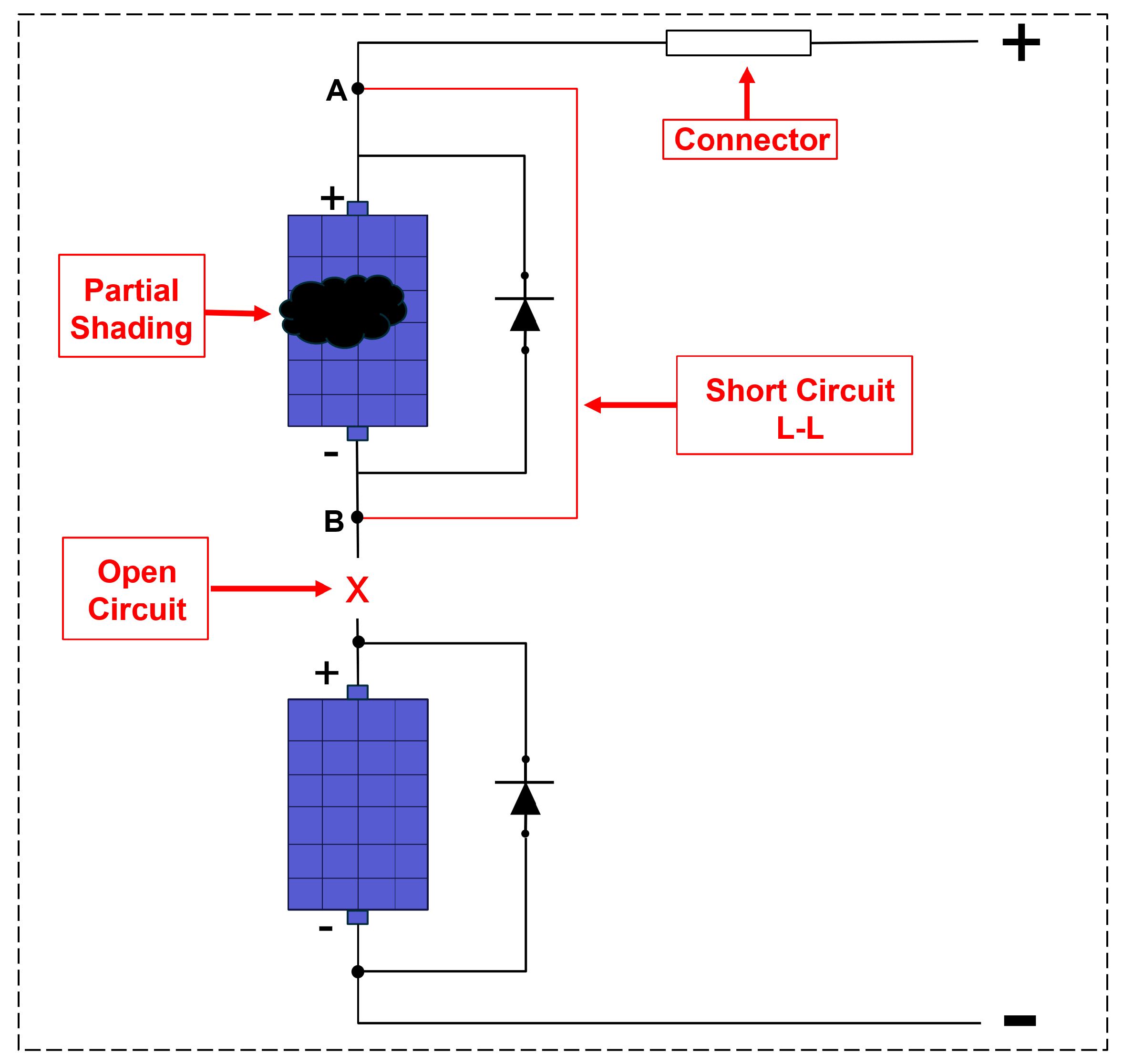
The primary impact of an open-circuit fault is the partial or complete loss of power output, thus degrading the overall efficiency of the PV system. In many cases, the fault may present intermittently, which complicates its identification and delays corrective action. Diagnostic methods such as infrared thermography, visual inspection, and continuity testing are typically employed to locate and confirm this fault. Figure 2 illustrates a schematic depiction of the open-circuit condition and its typical occurrence in PV systems.

2.2. Line-to-Line Short-Circuit Fault

Short-circuit faults occur when two points at different electrical potentials become directly connected, creating a low-impedance path for the current and resulting in excessive current flow [4]. This condition can cause a rapid temperature rise, potentially damaging components and creating severe fire hazards if left unmitigated.

In the specific case of a line-to-line short circuit, the fault involves an unintended connection between two conductors—typically of different polarities or phases—without sufficient impedance to restrict the current surge [6]. Such faults may originate from insulation breakdown, degraded cable sheathing, poor mechanical assembly, or accidental contact between conductors. On the DC side of PV systems, this type of fault is especially critical, as it can lead to sustained overheating of modules and accelerated degradation of both PV modules and inverters.

Preventive and corrective strategies include the use of overcurrent protection devices such as circuit breakers and fast-acting fuses, as well as routine visual and thermographic inspections to assess the integrity of the conductor insulation and connections. Figure 2 presents an illustration of this fault and its occurrence within a PV array.

2.3. Shading Effects

Although shading is not an electrical fault in the traditional sense, it has substantial implications for PV system performance. Shading may be classified as partial or permanent, depending on its duration and origin [11]. In both cases, shading can induce current mismatch among cells and modules, reduce energy yield, and promote localized heating—commonly referred to as “hot spots”—which can permanently damage modules.

Partial shading typically results from transient obstructions such as clouds, dust particles, or shadows cast by nearby moving objects. This causes non-uniform irradiance across the PV array, leading to uneven power generation and reduced inverter efficiency.

Permanent shading is caused by fixed objects such as buildings, vegetation, or structural elements being improperly positioned during system design. This chronic irradiance mismatch results in long-term energy losses and thermal stress on shaded cells. While bypass diodes can alleviate voltage drops by rerouting the current around shaded sections, they do not eliminate the associated power losses or mitigate the thermal effects completely.

To minimize the impact of shading, PV system design should include detailed site assessment, shadow modeling, and simulation tools that incorporate geographic, architectural, and solar path data. Figure 2 illustrates an example of shading due to clouds and its effect on power distribution across PV modules [12].

2.4. Connector Faults

Connector faults represent a frequent and critical failure mode in PV systems, particularly in large-scale installations. These faults often result from poor crimping, connector mismatches, environmental exposure (e.g., humidity, UV radiation), corrosion, or mechanical degradation due to thermal expansion and contraction [3].

In this work, connector faults were emulated by inserting a resistive element in series with the module interconnects, simulating increased contact resistance. This configuration enabled analysis of its impact on voltage drop, thermal dissipation, and characteristic curve deformation.

One of the most hazardous outcomes of connector degradation is the occurrence of arc faults—electrical discharges caused by intermittent or incomplete connections. Arcing can generate extreme localized heating and ignite nearby materials, particularly under continuous DC operation, where arcs are self-sustaining. If not rapidly interrupted, this condition can pose a substantial fire risk [3].

To mitigate connector-related issues, best practices include the use of high-quality, certified connectors with ingress protection (IP) ratings that make them suitable for outdoor use; regular thermographic inspections; and the deployment of arc fault circuit interrupters (AFCIs). Modern inverters equipped with diagnostic and fault detection capabilities can further enhance the system’s reliability and early fault identification. Figure 2 shows the fault simulation layout and the resulting modifications to the I–V curve.

3. Materials and Methods

This section outlines the methodological framework adopted in this study. It begins by presenting the model of the simulated photovoltaic (PV) system, followed by the specification of the components and parameters used to replicate realistic system behavior under both normal and fault conditions. Finally, the procedures for fault insertion and the modeling strategies employed for each fault type in the simulation environment are described in detail.

3.1. Simulated System Model

The simulation model was developed with consideration of two configurations: a single-string setup and a three-string configuration. Each string comprises seven PV modules connected in series. Figure 3 and Figure 4 illustrate the block diagrams created in Matlab/Simulink for both configurations.

Both configurations were designed to facilitate the extraction of current–voltage (I–V) and power–voltage (P–V) curves, enabling the generation of training and test datasets for the machine learning-based fault classification model. This dual-configuration approach supports both system-level analysis (three strings in parallel) and string-level diagnostics. During the commissioning process of photovoltaic power plants (PVPPs), it is common to analyze the I–V curve of each string individually, which allows for more precise localization and classification of faults without needing to evaluate the entire system [13].

3.2. Component Description and Parameters

The Simulink blocks used in the model and their key functions are illustrated in Figure 5, with their respective parameters described below:

• Block 01: Simulates a constant irradiance source affecting the PV modules.
• Block 02: Represents the photovoltaic module, which takes irradiance and temperature as inputs. The module parameters are listed in

  Table 1. Photovoltaic module parameters.

  Parameter	Value
  Parallel Strings	1
  Modules in Series per String	1
  Maximum Power (W)	559.8567
  Cells per Module (Ncell)	66
  Open-Circuit Voltage Voc (V)	47.42
  Short-Circuit Current Isc (A)	15.0
  Maximum Power Point Voltage Vmp (V)	39.51
  Maximum Power Point Current Imp (A)	14.17
  Temperature Coefficient of Voc (%/°C)	−0.25
  Temperature Coefficient of Isc (%/°C)	0.102

  .
• Block 03: Models the bypass diode used for hot spot protection. The diode parameters are shown in

  Table 2. Bypass diode parameters.

  Parameter	Value
  Resistance Ron (Ohms)	0.001
  Inductance Lon (H)	0
  Forward Voltage Vf (V)	0.7
  Initial Current Ic (A)	0
  Snubber Resistance Rs (Ohms)	inf
  Snubber Capacitance Cs (F)	inf

  .
• Block 04: Includes measurement instruments for current, voltage, and power, enabling I–V and P–V curve generation and fault detection.

3.3. Fault Implementation

Faults were modeled under different environmental and operating conditions to emulate real-world commissioning scenarios. The following subsections describe the implementation of each fault type.

3.3.1. Open-Circuit Fault

This fault was modeled by disconnecting two nodes in the first string using a Breaker block, which functions as a switch to simulate an open circuit. It was only applied in the three-string model, as a single string disconnection in the one-string configuration would completely interrupt current flow and power generation.

3.3.2. Partial Shading

Partial shading was introduced by applying reduced irradiance to specific modules. For the single-string configuration, irradiance values of 100, 200, and 300 W/m² were applied to modules 1, 3, and 6, respectively. In the three-string configuration, the same irradiance levels were assigned to modules 1, 8, and 15 (100 W/m²), modules 3, 10, and 17 (200 W/m²), and modules 6, 13, and 20 (300 W/m²).

3.3.3. Line-to-Line Short Circuit

This fault was implemented by placing a short-circuit block between two defined nodes (points A and B), as depicted in Figure 2.

3.3.4. Connector Fault

Connector faults were emulated by inserting resistors between adjacent modules. In the single-string model, resistances of 1, 2, and 3 Ω were added between modules 1 and 2, 3 and 4, and 6 and 7, respectively. In the three-string configuration, resistances were inserted as follows: 1 Ω between modules 1 and 2 and between modules 6 and 7; 2 Ω between modules 9 and 10 and between modules 11 and 12; and 3 Ω between modules 16 and 17 and between modules 19 and 20.

4. Proposed Fault Classification Method

This section presents the proposed methodology for classifying faults in photovoltaic (PV) systems. It begins with the process of database creation, including the extraction of relevant electrical features from I–V and P–V curves. It then addresses data preprocessing procedures such as normalization and labeling. Next, it outlines the multiclass classification techniques employed, with emphasis on the One-Versus-One (OVO) and One-Versus-Rest (OVR) strategies. Finally, the evaluation metrics used to validate the classification model are discussed.

4.1. Database Creation

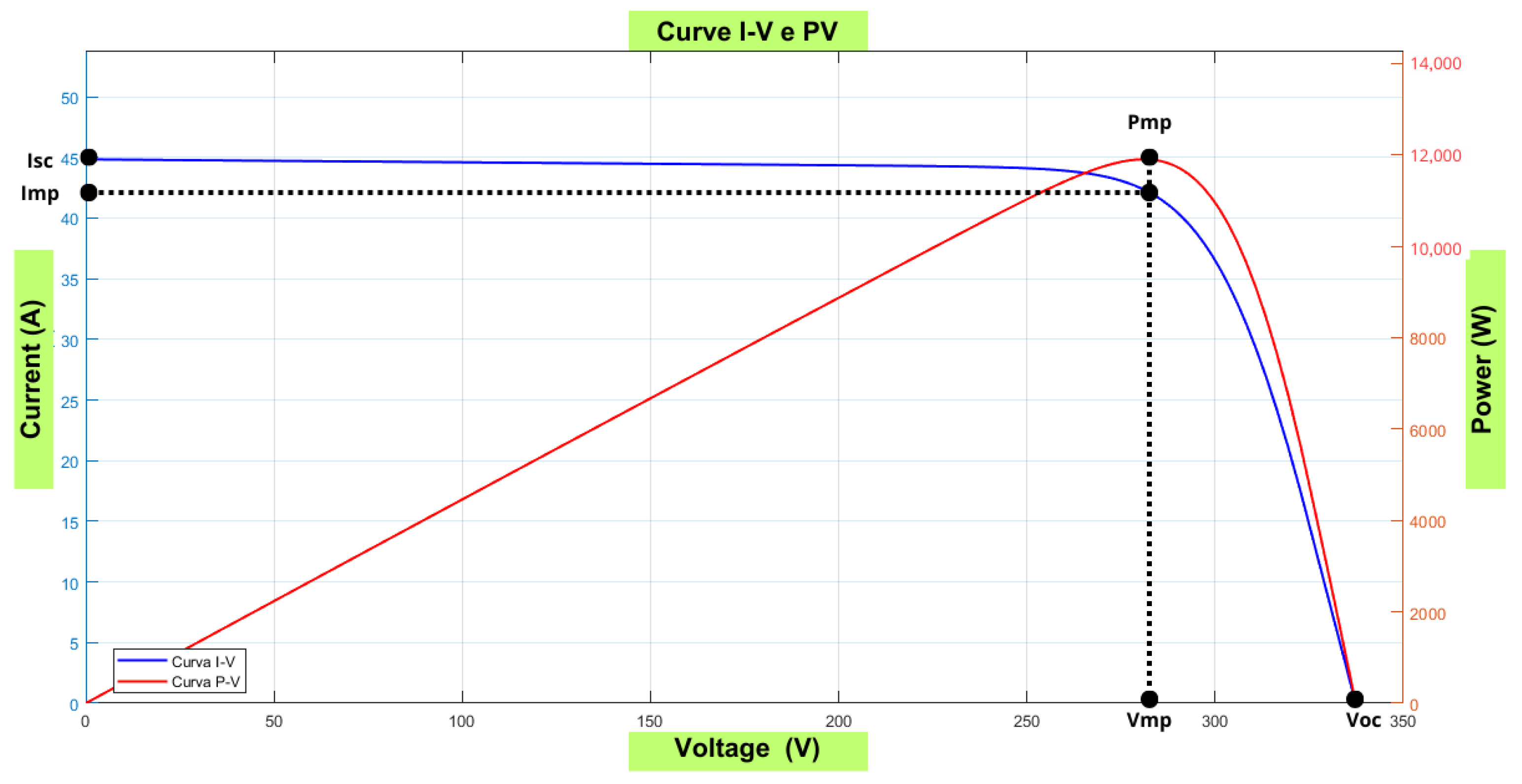
A structured methodology was developed to extract electrical parameters from I–V and P–V curves, thereby forming the basis of the dataset. The key features extracted include the short-circuit current ($I_{\mathrm{sc}}$), open-circuit voltage ($V_{\mathrm{oc}}$), current at maximum power point ($I_{\mathrm{mp}}$), voltage at maximum power point ($V_{\mathrm{mp}}$), and maximum power output ($P_{\mathrm{mp}}$), as illustrated in Figure 6.

The extraction was performed using a custom MATLAB algorithm, depicted in the flowchart shown in Figure 7.

The algorithm first initializes key parameters such as temperature and defines the structure for storing extracted features. A FOR loop iterates over temperature values from 20 °C to 35 °C in 1 °C increments. Within each temperature iteration, irradiance values are varied between 700 W/m² and 1000 W/m², with step sizes of 10 W/m², 20 W/m², and 30 W/m², ensuring a rich and diverse dataset.

At the end of the process, as outlined in the flowchart in Figure 7, an Excel-based dataset is generated containing the key features extracted from the I–V and P–V curves, as described in Figure 6, under varying irradiance and temperature levels. Additionally, the dataset includes records for different fault conditions, such as short-circuit, open-circuit, partial shading, connector fault, and normal operating conditions.

Table 3. An example of the database with different irradiance levels and a temperature of 20 °C.

Temp. (°C)	Irradiance (W/m2)	Voc (V)	Isc (A)	Pmax (W)	Imax (A)	Vmax (V)
20.00	1000.00	337.25	14.95	3966.57	14.11	281.15
20.00	980.00	336.92	14.65	3889.38	13.87	280.49
20.00	960.00	336.59	14.35	3812.00	13.57	280.82
20.00	940.00	335.92	14.05	3734.40	13.28	281.15
20.00	920.00	335.59	13.75	3656.63	12.99	281.49

presents an example of the dataset structure, considering a fixed temperature of 20 °C, irradiance variation in 20 W/m² increments, and the main extracted features: open-circuit voltage (V_oc), short-circuit current (I_sc), maximum power (P_max), current at maximum power point (I_max), and voltage at maximum power point (V_max). The implementation methods for all fault types are described in Section 3.3.

The entire feature extraction process for the dataset was performed on an Acer Aspire 5 notebook, equipped with a 10th-generation Intel Core i5 processor. MATLAB was used to execute the script described in Figure 7, with support from the Simulink environment. The simulated configurations for one and three PV strings are represented in Figure 3 and Figure 4, respectively.

Table 4. The total time for building the database, considering the types of faults and the number of samples per configuration.

Type	1 String (1984 Samples)	3 Strings (2480 Samples)
Normal condition	00:19:30	01:47:30
Shading	00:19:45	01:57:05
Short circuit	00:19:54	01:55:50
Connector fault	00:19:48	01:53:12
Open circuit		01:52:34
Total time	01:18:57	09:26:11

presents the total processing time required for dataset generation, using as examples the datasets with 1984 and 2480 samples for the single-string and three-string configurations, respectively.

4.2. Data Preprocessing

The complete dataset comprised 3712 samples for the single-string configuration and 4640 samples for the three-string configuration. Specifically, the single-string model used subsets of 704, 1024, and 1984 samples, while the three-string model used 880, 1280, and 2480 samples. In each case, the data were randomly partitioned into training (70%) and testing (30%) subsets.

The purpose of this data partitioning approach was to evaluate model performance across different dataset sizes, assess the model’s generalization capability under conditions that approximate real-world scenarios, and verify model stability—that is, whether the model delivers consistent results even with varying data volumes.

Each sample was labeled based on the operational conditions simulated in the PV circuit. In the single-string system, the following labels were assigned: 0 (normal), 1 (shading), 2 (short circuit), and 3 (connector failure). For the three-string configuration, an additional label 4 was used to represent open-circuit faults.

All features were normalized using the MinMaxScaler technique to rescale the feature values to a [0, 1] range:

$$x_{\mathrm{normalized}}={\displaystyle \frac{x-x_{\min }}{x_{\max }-x_{\min }}}$$

(1)

where x represents the original value, and $x_{\min }$ and $x_{\max }$ denote the minimum and maximum values within the dataset, respectively. This procedure prevented variables with different scales from disproportionately affecting the model.

4.3. Multiclass Classification

The classification problem was addressed using two widely adopted multiclass strategies, One-Versus-Rest (OVR) and One-Versus-One (OVO), which were originally applied to multiclass classification with Support Vector Machines (SVMs) by [14] and discussed in [15].

Both techniques were implemented using the $XGBClassifier$ algorithm, developed by [16], due to its robustness and high accuracy in supervised learning tasks.

4.3.1. OVR Multiclass Technique

In the OVR strategy, a separate binary classifier is trained for each class to distinguish it from all other classes. For a three-class problem ($C_1$, $C_2$, $C_3$), the following classifiers are trained:

• $scor{e}_1\left(x\right)$: Classifies $C_1$ vs. $C_2$ and $C_3$;
• $scor{e}_2\left(x\right)$: Classifies $C_2$ vs. $C_1$ and $C_3$;
• $scor{e}_3\left(x\right)$: Classifies $C_3$ vs. $C_1$ and $C_2$.

Each classifier computes a score:

$$scor{e}_k\left(x\right)=\sum _{m=1}^M\eta ·h_{k,m}\left(x\right)$$

where

• M: number of trees;
• $\eta$: learning rate;
• $h_{k,m}\left(x\right)$: output of m-th tree for class k.

Prediction Scoring: Each classifier returns a confidence score for its prediction:

• $scor{e}_1\left(x\right)$;
• $scor{e}_2\left(x\right)$;
• $scor{e}_3\left(x\right)$.

From the obtained scores, the probability of the input x belonging to a specific class k is determined using the following equation:

$$P_k\left(x\right)={\displaystyle \frac{1}{1+e^{-scor{e}_k\left(x\right)}}}$$

(2)

A logistic (sigmoid) function is used to transform the score $scor{e}_k\left(x\right)$ into a probability for class k.

The class with the highest score is selected. In this case,

• $C_1:0.7$;
• $C_2:0.2$;
• $C_3:0.9$.

The final predicted class is the one associated with the highest probability, determined by the following equation:

$$\widehat{y}=arg\underset{k}{max}{P}_k\left(x\right)$$

(3)

where $P_k\left(x\right)$ denotes the predicted probability of the input sample x belonging to class k.

Thus, x is classified as $C_3$, since it has the highest score. In this study, the $XGBClassifier$ algorithm (based on Gradient Boosting) was used for each subproblem generated by the OVR approach due to its high efficiency in supervised learning.

4.3.2. OVO Multiclass Technique

In the OVO strategy, a binary classifier is trained for each unique pair of classes. For three classes ($C_1$, $C_2$, $C_3$), the following classifiers are trained:

Trained Classifiers:

• $scor{e}_{12}\left(x\right)$: Classifies between $C_1$ and $C_2$.
• $scor{e}_{13}\left(x\right)$: Classifies between $C_1$ and $C_3$.
• $scor{e}_{23}\left(x\right)$: Classifies between $C_2$ and $C_3$.

Each classifier is trained using $XGBClassifier$, which uses multiple decision trees to produce a prediction score. The score for each binary classifier $scor{e}_{ij}\left(x\right)$ is computed as follows:

$$scor{e}_{ij}\left(x\right)=\sum _{m=1}^M\eta ·h_{ij,m}\left(x\right)$$

where

• M is the total number of decision trees;
• $\eta$ is the learning rate;
• $h_{ij,m}\left(x\right)$ is the output of the m-th tree in classifier $f_{ij}$.

The raw score is transformed into a probability using the sigmoid function:

$$P_{ij}\left(x\right)={\displaystyle \frac{1}{1+e^{-scor{e}_{ij}\left(x\right)}}}$$

The class prediction is then made as follows:

$${\widehat{y}}_{ij}=\left\{\begin{array}{cc}{C}_i,\hfill & \mathrm{if}{P}_{ij}\left(x\right)>0.5\hfill \\ C_j,\hfill & \mathrm{otherwise}\hfill \end{array}\right.$$

Each classifier votes for one class. The number of votes received by class $C_k$ is

$$Vote{s}_k\left(x\right)=\sum _{i=1}^K\sum _{j=i+1}^{K}1[{\widehat{y}}_{ij}=C_k]$$

where $1[·]$ is the indicator function, which returns 1 if the condition is true, and 0 otherwise.

The final predicted class is the one with the most votes:

$$\widehat{y}\left(x\right)=arg\underset{k}{max}Vote{s}_k\left(x\right)$$

The votes for each class are as follows:

• $C_1:1$ vote.
• $C_2:0$ votes.
• $C_3:2$ votes.

Since class $C_3$ received the highest number of votes among all classifiers, it was selected as the final predicted class. Similarly to the OVR approach, $XGBClassifier$ was used to solve each binary subproblem, ensuring model robustness.

Table 5. Comparison of One-Versus-One (OVO) and One-Versus-Rest (OVR).

Feature	OVO	OVR
Number of Classifiers	${\displaystyle \frac{K(K-1)}{2}}$	K
Complexity	Higher	Lower
Classification	Pairwise class comparison	Each class vs. all others

compares the two methods.

4.4. Evaluation Metrics

The model’s performance was evaluated using four metrics: accuracy, precision, sensitivity (recall), and the confusion matrix.

4.4.1. Accuracy

Accuracy measures the proportion of correct predictions relative to the total number of predictions made:

$$\mathrm{Accuracy}={\displaystyle \frac{\mathrm{TP}+\mathrm{TN}}{\mathrm{TP}+\mathrm{TN}+\mathrm{FP}+\mathrm{FN}}}$$

(4)

where:

• TP (True Positives): Correctly classified positive instances.
• TN (True Negatives): Correctly classified negative instances.
• FP (False Positives): Negative instances incorrectly classified as positive.
• FN (False Negatives): Positive instances incorrectly classified as negative.

4.4.2. Precision

Precision quantifies the proportion of correctly predicted positive instances relative to the total number of positive predictions made by the model:

$$\mathrm{Precision}={\displaystyle \frac{\mathrm{TP}}{\mathrm{TP}+\mathrm{FP}}}$$

(5)

4.4.3. Sensitivity

Sensitivity, also known as recall, measures the proportion of actual positive instances that are correctly identified:

$$\mathrm{Recall}={\displaystyle \frac{\mathrm{TP}}{\mathrm{TP}+\mathrm{FN}}}$$

(6)

4.4.4. Confusion Matrix

The confusion matrix (

Table 6. Confusion matrix.

	Predicted Positive	Predicted Negative
Actual Positive	TP	FN
Actual Negative	FP	TN

) provides an overview of the model’s performance by comparing correct and incorrect predictions for each class.

These metrics offer a comprehensive evaluation of the model’s performance, serving as essential indicators for assessing its effectiveness, particularly in scenarios with imbalanced class distributions.

5. Results and Analysis

This section presents the results obtained from the analysis of voltage and power characteristics in photovoltaic (PV) systems operating under both normal and faulty conditions. The fault scenarios implemented, as described in Section 3, were evaluated using I–V and P–V curves. Figure 8 illustrates the distinct behaviors observed across different operating conditions.

The analysis highlights the substantial influence that different fault types have on PV system performance. These anomalies directly affect current and voltage behavior, resulting in power losses and reduced operational stability. Accurate interpretation of these deviations is essential for reliable fault detection and efficient system maintenance.

5.1. Normal Operating Conditions

Under normal operating conditions, represented by the blue curve in Figure 8a, the PV system demonstrates expected behavior, with the maximum current ($I_{\max }$) and voltage ($V_{\max }$) occurring near the short-circuit and open-circuit regions, respectively. The corresponding P–V curve in Figure 8b exhibits a single, well-defined Maximum Power Point (MPP), indicating optimal energy harvesting.

5.2. Connector Fault

The connector fault, represented by the red curve, leads to a significant reduction in the maximum current due to increased contact resistance or partial interruption of current flow (Figure 8a). Consequently, the P–V curve (Figure 8b) shows a notable decrease in maximum power generation, indicating a moderate impact on system performance.

5.3. Shading Fault

Under shading conditions, illustrated by the orange curve in Figure 8a, multiple “steps” can be observed in the I–V curve. This phenomenon occurs due to the uneven distribution of shadows across different cell strings, leading to a reduction in the system’s total current. In the P–V curve (Figure 8b), the presence of multiple power peaks indicates challenges in identifying the Maximum Power Point (MPP), ultimately reducing the system’s efficiency.

5.4. Line-to-Line Short-Circuit Fault

The line-to-line short-circuit fault, represented by the purple curve in Figure 8a, causes a sudden drop in both voltage and current. The I–V curve rapidly converges to values close to zero, while the P–V curve (Figure 8b) exhibits a significant decline in generated power, severely compromising system operation.

5.5. Open-Circuit Fault

In the case of an open-circuit fault, represented by the green curve in Figure 8a, the current is drastically reduced, whereas the voltage remains close to its nominal value. In the P–V curve, a decrease in maximum power is observed due to the lack of contribution from the affected string.

5.6. Fault Classification Using a Single String

A classification model was developed using a dataset comprising 3712 samples collected from a single PV string, as illustrated in Figure 3. The dataset was divided into three subsets containing 704, 1024, and 1984 samples. This setup demonstrates simplicity and feasibility for field applications, ensuring accurate fault detection with limited instrumentation.

Classification results for four categories—normal conditions, shading fault, connector fault, and line-to-line short-circuit fault—are presented in

Table 7. Performance metrics for single-string classification.

Metric	OVR Technique			OVO Technique
	704	1024	1984	704	1024	1984
Accuracy (%)	100	99.67	99.83	100	99.03	99.83
Sensitivity (%)	100	99.67	99.83	100	99.03	99.83
Precision (%)	100	99.68	99.83	100	99.05	99.83

. The model was tested using two strategies: One-Versus-Rest (OVR) and One-Versus-One (OVO), both based on XGBoost classifiers. Notably, both approaches achieved 100% accuracy on the smallest dataset (704 samples).

The results indicate that both classification techniques achieved excellent performance with the different types of data, with an average accuracy of 99.83% for OVR and 99.62% for OVO.

The confusion matrices, presented in Figure 9 and Figure 10, illustrate the classification errors for both classifiers, OVR and OVO, respectively.

5.7. Fault Classification Using Three Strings

In a more complex configuration, a model comprising three PV strings (as illustrated in Figure 4) was evaluated using a dataset of 4640 samples divided into subsets of 880, 1280, and 2480 samples. The classification process included an additional category: open-circuit fault.

The analysis of the results presented in

Table 8. Performance metrics for three-string classification.

Metric	OVR Technique			OVO Technique
	880	1280	2480	880	1280	2480
Accuracy (%)	98.86	99.48	100	97.35	99.48	100
Sensitivity (%)	98.86	99.48	100	97.35	99.48	100
Precision (%)	98.93	99.49	100	97.35	99.48	100

indicates that both models, OVR and OVO, exhibited nearly identical performance, achieving 100% accuracy on the subset with 2480 samples. Precision and sensitivity showed slight variation between the OVR and OVO techniques on the subsets of 880 and 1280 samples.

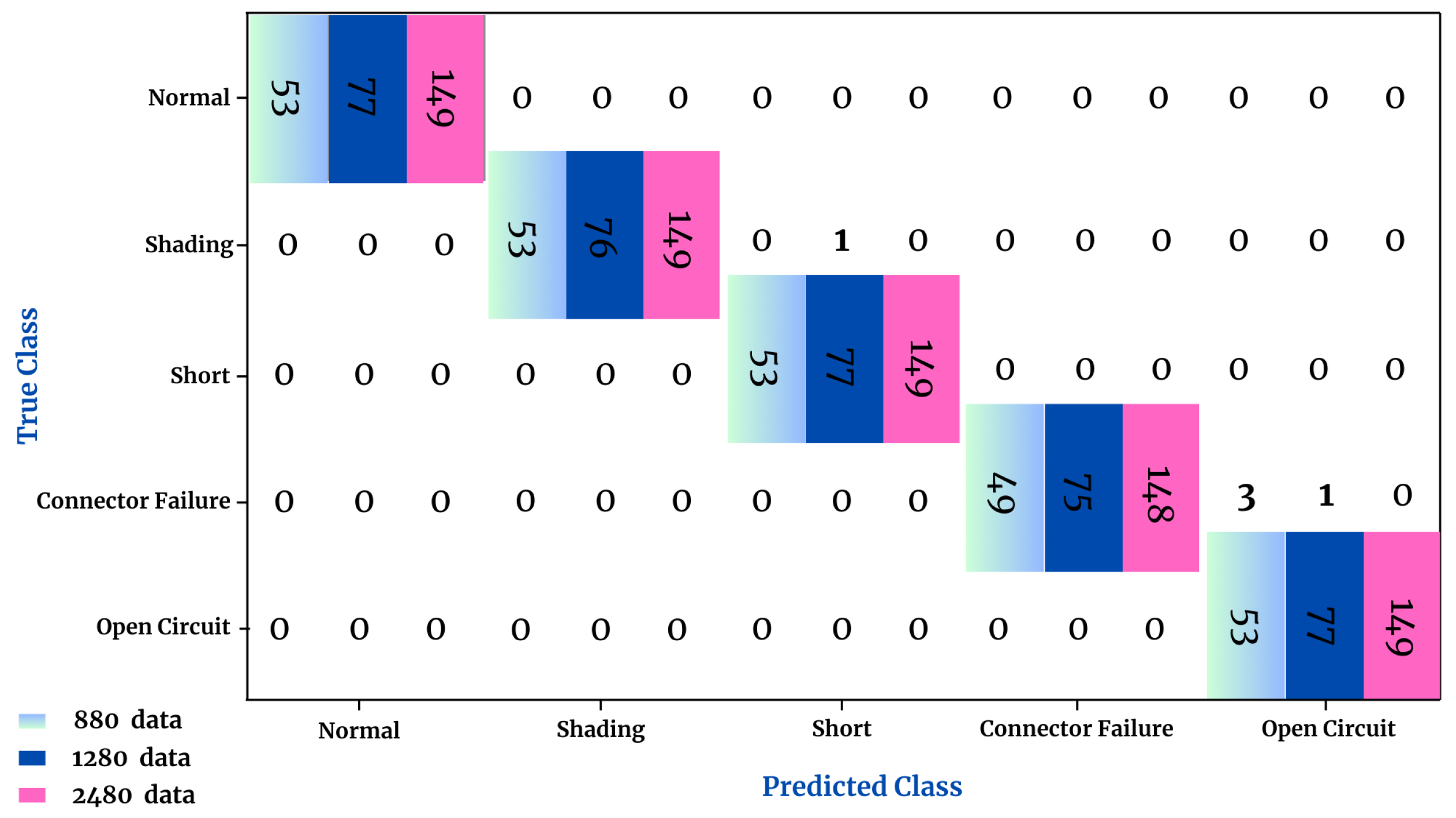
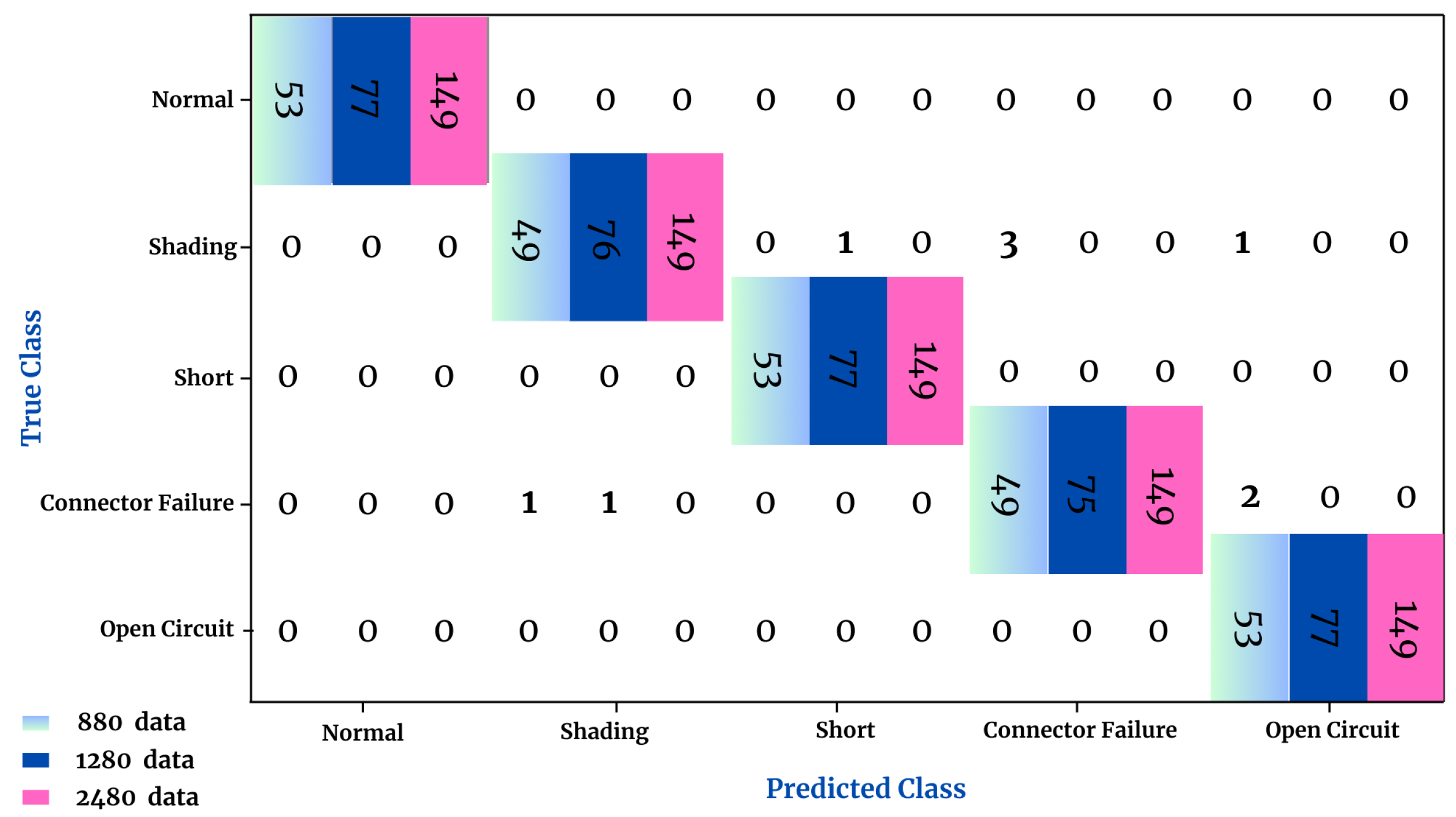
Figure 11 and Figure 12 show the confusion matrices for the OVR and OVO approaches, confirming the classification accuracy for the multi-string configuration.

The values shown in Figure 9, Figure 10, Figure 11 and Figure 12 correspond to the confusion matrices obtained from the experiments. Each value represents the number of samples correctly classified (diagonal entries) or misclassified (off-diagonal entries), indicating whether the predicted class matches the true class, based on the quantity of data evaluated.

Overall, the OVR technique exhibited slightly superior performance in terms of average accuracy across both configurations: single-string and three-string.

Regarding training time, considering the datasets with 1984 and 2480 samples for the single-string and three-string configurations, respectively, the results are presented in

Table 9. The training time, in milliseconds, for the OVR and OVO approaches under the single-string and three-string configurations.

Configuration	Number of Samples	OVR	OVO
Single string	1984	167 (ms)	135 (ms)
Three strings	2480	227 (ms)	236 (ms)

.

In general, the OVR technique tends to be more computationally efficient for larger datasets, as it requires only K classifiers for K classes, whereas the OVO approach demands $K(K-1)/2$ classifiers.

6. Conclusions

This study analyzed and classified faults in a photovoltaic power plant using the MATLAB/Simulink environment, focusing on the direct current (DC) side. The implementation of robust fault detection and classification methodologies proved essential for optimizing the commissioning, operation, and maintenance (O&M) processes, thereby minimizing technical and economic impacts.

The analysis considered the characteristics of an 11.76 kWp photovoltaic power plant located in Pesqueira, Pernambuco, under different environmental conditions. The I–V and P–V curve results revealed distinct patterns for each type of fault, indicating that short-circuit faults are the most severe, while connector faults, although initially less impactful, can evolve into critical issues if not detected early.

Shading faults resulted in multiple Maximum Power Points, complicating system operation, while open-circuit faults caused significant reductions in current and power output. The classification tests, considering three data subsets, achieved average accuracies exceeding 99.83% and 99.62% with the One-Versus-Rest (OVR) and One-Versus-One (OVO) techniques, respectively, using a single string. For three strings, the results were 99.44% (OVR) and 98.94% (OVO), validating the effectiveness of the proposed method and demonstrating a low error rate across the evaluation metrics.

Unlike previous studies, this work emphasizes the importance of integrating fault detection and classification systems during the commissioning phase, incorporating environmental variability and expanding the practical applicability of multiclass machine learning techniques in the photovoltaic sector.

For future work, it is recommended to validate the methodology using real-world data from operational systems, implement it in the field to assess its robustness under actual conditions, and develop solutions for real-time fault detection, enabling faster and more efficient preventive responses in the context of solar power plant operation and maintenance.

References

1. Gokgoz, M.; Saglam, S.; Oral, B. Challenges during commissioning and operation in photovoltaic power plants by electrical faults. Turk. J. Electromech. Energy 2023, 8, 37–44. [Google Scholar]
2. Lazzaretti, A.E.; Costa, C.H.d.; Rodrigues, M.P.; Yamada, G.D.; Lexinoski, G.; Moritz, G.L.; Oroski, E.; Goes, R.E.d.; Linhares, R.R.; Stadzisz, P.C.; et al. A Monitoring System for Online Fault Detection and Classification in Photovoltaic Plants. Sensors 2020, 20, 4688. [Google Scholar] [CrossRef] [PubMed]
3. Hojabri, M.; Kellerhals, S.; Upadhyay, G.; Bowler, B. IoT-Based PV Array Fault Detection and Classification Using Embedded Supervised Learning Methods. Energies 2022, 15, 2097. [Google Scholar] [CrossRef]
4. Gökgöz, M.; Sağlam, Ş.; Oral, B. Investigation of Failures during Commissioning and Operation in Photovoltaic Power Systems. Appl. Sci. 2024, 14, 2083. [Google Scholar] [CrossRef]
5. Cassini, D.A.; Costa, S.C.S.; Diniz, A.S.A.C.; Kazmerski, L.L. Analysis of the Soiling Effects on Commissioning of Photovoltaic Systems: Short-Circuit Current Correction. In Proceedings of the Congresso Brasileiro de Energia Solar (CBENS), Florianópolis, Brazil, 23–27 May 2022; pp. 1–8. [Google Scholar] [CrossRef]
6. Memon, S.A.; Javed, Q.; Kim, W.-G.; Mahmood, Z.; Khan, U.; Shahzad, M. A Machine-Learning-Based Robust Classification Method for PV Panel Faults. Sensors 2022, 22, 8515. [Google Scholar] [CrossRef] [PubMed]
7. Líbano, F.B.; de Lima Silva, L.A.; de Freitas, E.P. Fault Detection in Photovoltaic Systems Using a Machine Learning Approach. IEEE Access 2025, 13, 41406–41421. [Google Scholar] [CrossRef]
8. Nassreddine, G.; El Arid, A.; Nassereddine, M.; Al Khatib, O. Fault Detection and Classification for Photovoltaic Panel System Using Machine Learning Techniques; John Wiley Sons Ltd.: Hoboken, NJ, USA, 2025; Volume 13. [Google Scholar] [CrossRef]
9. Suliman, F.; Anayi, F.; Packianather, M. Electrical Faults Analysis and Detection in Photovoltaic Arrays Based on Machine Learning Classifiers. Sustainability 2025, 16, 1102. [Google Scholar] [CrossRef]
10. Quiles-Cucarella, E.; Sánchez-Roca, P.; Agustí-Mercader, I. Performance Optimization of Machine-Learning Algorithms for Fault Detection and Diagnosis in PV Systems. Eletronics 2025, 14, 1709. [Google Scholar] [CrossRef]
11. Berghout, T.; Benbouzid, M.; Bentrcia, T.; Ma, X.; Djurović, S.; Mouss, L.-H. Machine Learning-Based Condition Monitoring for PV Systems: State of the Art and Future Prospects. Energies 2021, 14, 6316. [Google Scholar] [CrossRef]
12. Appiah, A.Y.; Zhang, X.; Ayawli, B.B.K.; Kyeremeh, F. Long Short-Term Memory Networks Based Automatic Feature Extraction for Photovoltaic Array Fault Diagnosis. IEEE Access 2020, 7, 30089–30101. [Google Scholar] [CrossRef]
13. Francisco Lisboa Santos, H.; Vassalo Maia da Costa, P.; Ouverney Torres de Sá Bezerra Pires, F.; Osório Regnier, L. Contornando as LimitaçõEs da Nbr-16274:2014 na AvaliaçãO de Desempenho e no Ajuste das SimulaçõEs de Sistemas Fotovoltaicos de Pequeno e MéDio Porte. In Proceedings of the Congresso Brasileiro de Energia Solar (CBENS), Florianópolis, Brazil, 23–27 May 2022. [Google Scholar] [CrossRef]
14. Weston, J.; Watkins, C. Support Vector Machines for Multi-Class Pattern Recognition. In Proceedings of the ESANN’1999 Proceedings—European Symposium on Artificial Neural Networks, Bruges, Belgium, 21–23 April 1999; pp. 219–224. [Google Scholar]
15. Hastie, T.; Tibshirani, R.; Jerome, J. The Elements of Statistical Learning: Data Mining, Inference, and Prediction, 2nd ed.; Springer: New York, NY, USA, 2009. [Google Scholar]
16. Chen, T.; Guestrin, C. XGBoost: A scalable tree boosting system. In Proceedings of the 22nd ACM SIGKDD International Conference on Knowledge Discovery and Data Mining, San Francisco, CA, USA, 13–17 August 2016; ACM: New York, NY, USA, 2016; pp. 785–794. [Google Scholar] [CrossRef]
Figure 1. Faults in photovoltaic systems on the DC side.
Energies 18 04681 g001
Figure 2. Open-circuit fault, line-to-line short circuit, connector failure, and ground fault.
Energies 18 04681 g002
Figure 3. A block diagram of the simulated PV system with a single string.
Energies 18 04681 g003
Figure 4. A block diagram of the simulated PV system with three strings.
Energies 18 04681 g004
Figure 5. The Simulink blocks employed in the simulation model.
Energies 18 04681 g005
Figure 6. Feature extraction from I–V and P–V curves.
Energies 18 04681 g006
Figure 7. A flowchart of the MATLAB algorithm for feature extraction from I–V curves.
Energies 18 04681 g007
Figure 8. Comparison of normal and fault conditions.
Energies 18 04681 g008
Figure 9. OVR—confusion matrix for single-string classification.
Energies 18 04681 g009
Figure 10. OVO—confusion matrix for single-string classification.
Energies 18 04681 g010
Figure 11. OVR—confusion matrix for three-string classification.
Energies 18 04681 g011
Figure 12. OVO—confusion matrix for three-string classification.
Energies 18 04681 g012