Article

An Adaptive Multi-Task Gaussian Process Regression Approach for Harmonic Modeling of Aggregated Loads in High-Voltage Substations

1
College of Electrical Engineering, Sichuan University, Chengdu 610065, China
2
Chengdu Electric Power Supply Company, State Grid Sichuan Power Supply Company, Chengdu 610041, China
*
Author to whom correspondence should be addressed.
Energies 2025, 18(17), 4670; https://doi.org/10.3390/en18174670
Submission received: 7 July 2025 / Revised: 8 August 2025 / Accepted: 18 August 2025 / Published: 3 September 2025

Abstract

To address the challenges of complex harmonic characteristics, multi-source coupling, and strong time variability in aggregated loads downstream of high-voltage substations, this paper proposes an Adaptive Multi-Task Gaussian Process Regression (AMT-GPR) method for harmonic modeling. First, field measurements from the medium-voltage side of a 500 kV substation are denoised and analyzed using Fourier transform to reveal the dynamic patterns and interdependencies of harmonic current magnitudes. Then, a multi-task GPR framework is constructed, incorporating task correlation modeling and adaptive kernel functions to capture inter-task coupling and differences in feature scales. Finally, a probabilistic harmonic model is developed based on multiple sets of measured data, and the modeling performance of AMT-GPR is compared with single-task GPR, conventional MT-GPR, and mainstream machine learning approaches including RBF, LS-SVM, and LSTM. Simulation results demonstrate that traditional harmonic modeling methods are insufficient to capture the dynamic behavior and uncertainty of aggregated loads and AMT-GPR maintains strong robustness under small-sample conditions, significantly reduces prediction errors, and yields narrower uncertainty intervals, outperforming the baseline models. These findings validate the effectiveness of the proposed method in modeling harmonics of aggregated loads in high-voltage substations and provide theoretical support for subsequent harmonic assessment and mitigation strategies.

1. Introduction

With the widespread deployment of nonlinear loads and power electronic devices in power systems, the complexity and impact of harmonic issues have increased significantly. Harmonics not only degrade power quality but also pose systemic risks such as equipment resonance and protection malfunctions [1,2,3,4,5]. The mechanisms behind harmonic generation in modern power systems have evolved beyond traditional load-side or local circuit characteristics, now encompassing system-wide coupling effects involving power sources, network topology, and load behaviors. Against this backdrop, high-accuracy modeling of harmonic sources has become a critical requirement for ensuring the safe and stable operation of power systems.
Current harmonic source modeling methods can be broadly categorized into model-driven and data-driven approaches, each with distinct advantages and limitations. Model-driven methods are grounded in circuit theory of power electronic devices and aim to analytically describe the nonlinear behavior of harmonic sources through equivalent circuit models, such as switching function models and state-space models. These approaches can be further divided into two subcategories: (1) Generic models typically represent harmonic sources as harmonic-controlled sources based on fundamental current control [6] and describe harmonic voltage–current coupling characteristics using equivalent circuits or Norton’s theorem [7,8,9]. Recent studies have introduced coupled admittance matrices to capture inter-harmonic interactions [10,11,12,13,14,15] and applied optimization techniques such as partial least squares [14] to address parameter identification challenges caused by collinearity. However, such models often lack the flexibility to dynamically represent time-varying harmonic behaviors and require re-identification of parameters for different devices and operating conditions. (2) Specific models are developed based on the physical mechanisms of particular harmonic sources, such as electric arc furnaces or wind power inverters, offering higher modeling accuracy. For instance, electric arc furnace models based on stochastic processes and chaos theory [16,17,18,19,20] effectively characterize the dynamic uncertainties of arc behavior; harmonic models of doubly-fed induction generators (DFIGs) [21,22] reveal the relationship between stator-side harmonics and control parameters; and the dead-time effects and frequency coupling mechanisms in grid-connected inverters have been extensively investigated [23], leading to the development of dead-time-coupled harmonic source models that describe the propagation of harmonic voltages through outer control loops, inner current loops, and phase-locked loops (PLLs). Nonetheless, the applicability of specific models is often limited to their corresponding scenarios, making them difficult to generalize across diverse types of harmonic sources.
Data-driven methods leverage machine learning and statistical analysis techniques to extract nonlinear mapping relationships from harmonic monitoring data without relying on prior circuit knowledge, making them well-suited for scenarios involving multiple coupled harmonic sources. Traditional approaches such as weighted least squares [24,25], partial least squares [26,27], and complex linear regression [28,29] enhance noise resistance through optimization algorithms but fail to fully capture the dynamic characteristics of harmonics. In recent years, neural networks have emerged as a prominent research direction. Radial basis function (RBF) networks [30,31] reduce computational complexity through adaptive structural adjustments; improved autoregressive networks [32] and generalized regression networks [33] integrate multi-frequency features to enhance dynamic modeling capabilities; and deep learning techniques, such as hybrid models combining convolutional neural networks (CNNs) and long short-term memory (LSTM) networks [34], further strengthen the representation of time-varying features. Nevertheless, data-driven methods still face challenges including limited interpretability of physical mechanisms, insufficient online adaptability, and high computational demands.
Aggregated loads downstream of high-voltage substations typically consist of numerous heterogeneous nonlinear devices, whose harmonic characteristics exhibit the following complexities: (1) multi-source coupling effects, where the superposition of harmonic emissions from different loads leads to a nonlinear enhancement of the overall harmonic distribution; (2) dynamic uncertainty, where random factors such as load switching and operational condition changes cause the harmonic spectrum to vary over time; and (3) small-sample challenges, where the difficulty in obtaining harmonic data from certain loads hinders the generalization capability of modeling approaches. Traditional harmonic modeling methods are mostly based on deterministic assumptions, making them inadequate for capturing the dynamic behavior and uncertainties of aggregated loads. These limitations are particularly pronounced in high-voltage substation scenarios, where multiple stochastic factors coexist. Therefore, developing a modeling approach capable of accurately characterizing the harmonic behavior of aggregated loads in high-voltage substations has become a critical focus in harmonic modeling research.
Multi-Task Gaussian Process Regression (MT-GPR), as an advanced machine learning technique, is well-suited for handling multivariate, nonlinear, and uncertain data, offering strong generalization capabilities and high predictive accuracy. Its core advantage lies in leveraging the correlation information shared among tasks to enhance overall model performance, making it particularly suitable for harmonic modeling of aggregated loads with common characteristics and dynamic behavior.
Based on the complex harmonic relationships observed in actual data, where conventional MT-GPR fails to dynamically adjust the correlations among different harmonic current components, this paper proposes an aggregated load harmonic modeling method for high-voltage substations. To address the time-varying harmonic characteristics of aggregated loads in high-voltage substations, this paper proposes a harmonic modeling method based on Adaptive Multi-Task Gaussian Process Regression (AMT-GPR). First, field measurement data from a high-voltage substation are collected and analyzed, revealing that different harmonic orders exhibit distinct temporal features. Second, a correlation analysis of harmonic current components indicates the presence of coupling relationships, particularly among odd-order harmonics. Then, by incorporating adaptive kernel functions and a multi-task learning framework, the Gaussian Process Regression model effectively captures the inter-task coupling while adaptively accommodating feature differences across harmonic orders. This enables the construction of a probabilistic harmonic model for aggregated loads in high-voltage substations, significantly improving prediction accuracy and model robustness. Finally, the proposed method is validated through a comparative analysis between simulation results and real-world measurement data, demonstrating its accuracy and reliability in practical applications.

2. Measured Data Analysis

This study conducts a harmonic characteristic analysis based on actual operational data from multiple 500 kV high-voltage substations. The measurement points are located at the medium-voltage side (220 kV) of high-voltage transformers, directly capturing the harmonic characteristics on the load side. The data consist of three-phase voltage and current waveform recordings over several consecutive days from multiple substations, as illustrated in Figure 1. A total of 22 sets of 24 h measurement data were collected from eight different monitoring points, with individual recording durations ranging from 1 to 3 days. These datasets cover typical weekday load variations and comprehensively reflect the harmonic behavior under various loading conditions.
To ensure the accuracy and reliability of the harmonic analysis, the collected raw data were systematically preprocessed. The main steps and methods are as follows:

2.1. Denoising

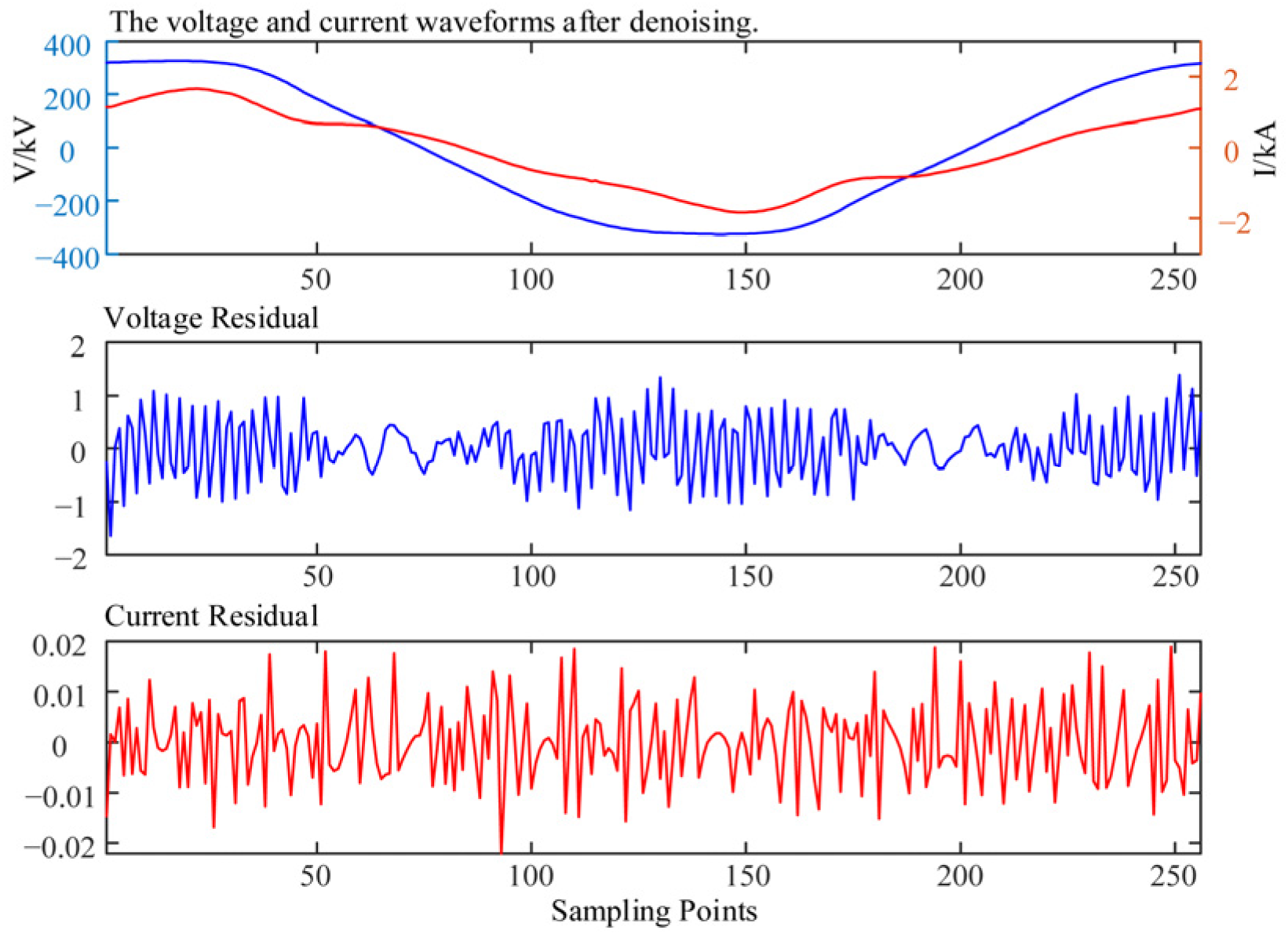
The raw data often contain high-frequency noise and outliers, which can compromise the accuracy of harmonic analysis. Wavelet transform (WT) was employed to denoise the voltage and current waveform data. The wavelet transform is defined by the following equation:
W ( a , b ) = 1 a x ( t ) ψ t b a d t
Here, x(t) represents the original signal, and ψ(t) denotes the mother wavelet function. The wavelet transform is governed by the scale parameter a and the translation parameter b. By selecting an appropriate wavelet basis function, the signal can be decomposed into sub-signals across different frequency bands, allowing high-frequency noise components to be removed while retaining the essential signal information. The denoised voltage and current waveforms, along with the residuals, are shown in Figure 2.
As shown in Figure 2, the residuals of both voltage and current exhibit small fluctuations with relatively uniform distribution, indicating that the denoised signals effectively retain their original characteristics while the noise components have been successfully separated. No apparent periodic patterns or abnormal spikes are observed, suggesting that the denoising process effectively removed high-frequency noise and random disturbances.

2.2. Harmonic Extraction

To investigate the harmonic characteristics on the low-voltage side of high-voltage substations, discrete Fourier transform (DFT) is applied to the measured waveform data for spectral analysis, enabling the extraction of fundamental and harmonic components of the voltage and current signals. For signals sampled at 256 points per cycle, the DFT is calculated using the following equation:
X ( k ) = n = 0 N 1 x ( n ) e j 2 π N k n
Here, N denotes the number of sampling points (with N = 256), k is the frequency index, and X(k) represents the signal in the frequency domain. To reduce spectral leakage effects, a Henning window (HW) is applied during the windowing process. The window function is defined as follows:
w ( n ) = 0.5 1 cos 2 π n N 1
The extracted harmonic frequency range spans from the fundamental frequency (50 Hz) up to the 12th harmonic (600 Hz).
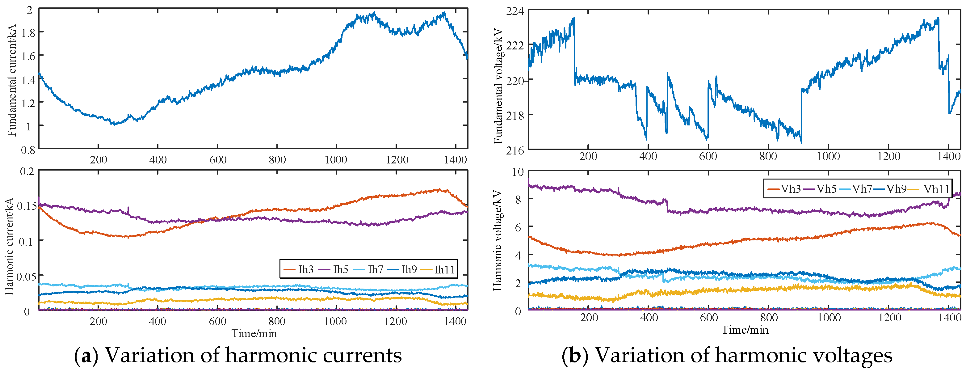
DFT analysis was performed on one-minute monitoring data over the course of a full day. Figure 3 illustrates the variation in harmonic characteristics of aggregated loads at a typical high-voltage substation.
From the figure above, the following observations can be made: (1) the fundamental current and voltage exhibit non-stationary time series characteristics; (2) the amplitudes of the third and fifth harmonic currents and voltages are significantly higher than those of other harmonic orders; (3) harmonics with larger amplitudes, such as the third harmonic, show notable fluctuations in both voltage and current; and (4) even-order harmonic components are approximately zero. Therefore, this study focuses on the 3rd, 5th, 7th, 9th, and 11th harmonics.
In practical power system harmonic analysis, harmonic amplitude is a key indicator for evaluating the severity of harmonic distortion. It directly reflects the degradation level of power quality and has a significant impact on equipment operation, system stability, and user safety. In contrast, harmonic phase angles generally have a less pronounced effect on the overall system, especially in scenarios involving multiple harmonic sources, where their influence becomes increasingly complex due to variations in system topology and load characteristics. Hence, from an engineering perspective, this study concentrates on the analysis and modeling of harmonic amplitudes to streamline the research scope and enhance its feasibility and practical value.
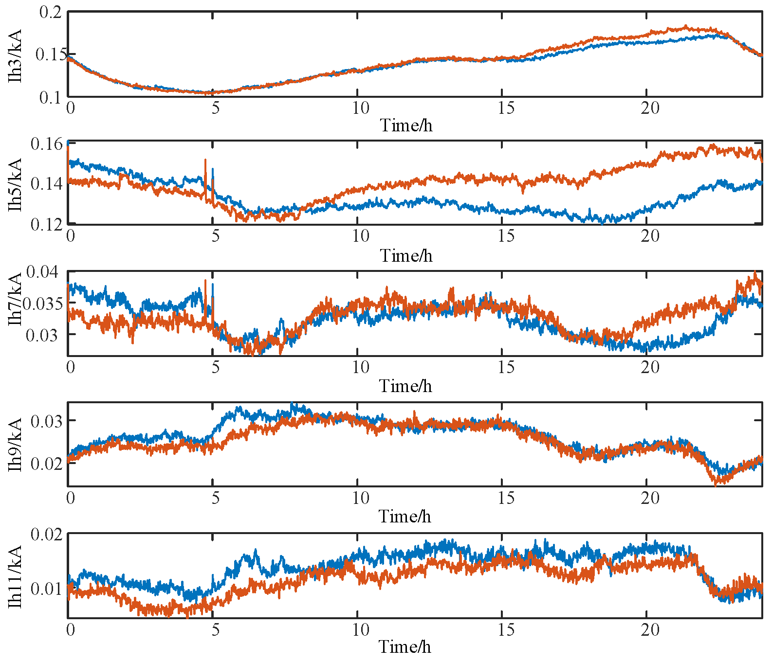
For aggregated nonlinear loads in high-voltage substations, the time-varying characteristics of harmonic currents exhibit notable regularity and complexity. The harmonic current profiles from two consecutive days at the same substation are shown in Figure 4.
Analysis of the harmonic current curves reveals that the amplitude variations across different harmonic orders are relatively smooth. This indicates that the fluctuations in harmonic currents are primarily influenced by the overall system load conditions rather than by instantaneous variations in individual local loads, making it difficult to accurately distinguish between different operating states using traditional methods such as abrupt change detection. Additionally, the harmonic profiles for two consecutive days at the same substation exhibit strong similarity. For instance, the third harmonic current consistently peaks during the same time window (e.g., 18:00–22:00) on both days and shows comparable fluctuation patterns during other periods. This suggests that the variation in harmonic currents follows a temporal continuity and periodic pattern, likely driven by daily cyclic load behaviors, such as those associated with industrial activities or residential electricity consumption.
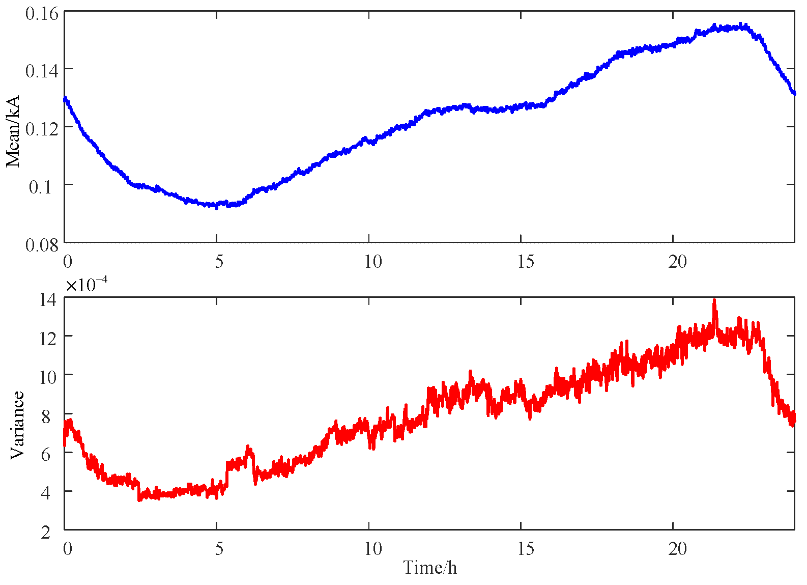
To further investigate the time-varying nature of harmonics, this study focuses on the statistical characteristics and variation patterns of harmonic amplitudes. Time-series analysis of harmonic currents over multiple consecutive days at the same substation is performed to extract statistical indicators such as mean and variance, thereby quantifying the fluctuation range. Figure 5 illustrates the statistical characteristics of the third harmonic current at a high-voltage substation, including its mean and variance, with the curves representing the temporal trends of these statistical features.
From Figure 5, the following observations can be made: (1) The mean curve of the harmonic current is relatively smooth, with the third harmonic current maintaining a mean value between approximately 91.7 A and 155.7 A over the 24 h period, indicating considerable long-term variation in the overall harmonic current level. (2) The variance curve reflects the degree of fluctuation in the harmonic current. The variance of the third harmonic current peaks between 18:00 and 22:00, suggesting that the fluctuation range is greatest during the evening load peak, while it remains relatively stable during other periods. By correlating harmonic amplitude data with load curves and relevant operational parameters, the relationship between harmonic amplitude and system operating conditions is analyzed. The results show that the time-varying characteristics of harmonic amplitudes are closely associated with load variations, with more pronounced fluctuations observed during peak load periods.

3. General Probabilistic Harmonic Model Based on Adaptive Multi-Task Gaussian Process Regression

3.1. Gaussian Process Regression

Gaussian Process Regression (GPR), as a non-parametric regression method based on Bayesian theory, is capable of handling complex nonlinear relationships while quantifying the uncertainty of predictions through Gaussian distributions. GPR has been widely applied across various fields such as machine learning, signal processing, and data mining, particularly in tasks requiring high prediction accuracy and uncertainty estimation. One of the core advantages of GPR is its ability to directly model the functional relationship between inputs and outputs while providing confidence intervals for the predicted values. Moreover, GPR does not assume any specific distribution for the data, offering strong flexibility and adaptability.
A Gaussian process defines the relationship among random variables in a function space using a Gaussian distribution. For an input vector X = [ x 1 , x 2 , , x n ] and output vector y = [ y 1 , y 2 , , y n ] , a Gaussian process is defined as follows:
y i = f ( x i ) , f ~ G P ( m ( x ) , k ( x , x ) )
where m(x) is the mean function, and k ( x , x ) is the covariance function.
When constructing a general model of harmonic sources within the framework of Gaussian Process Regression (GPR), the key lies in the appropriate design of the mean and covariance functions. According to theoretical analysis, the functional relationship between harmonic current and voltage can be expressed as follows:
I ˙ h = F h ( C , U ˙ 1 , U ˙ 2 , , U ˙ s )
Here, U ˙ s denotes the phasor of the sth harmonic voltage, C represents the current operating condition parameters, Fh denotes the functional relationship, and I ˙ h denotes the phasor of the hth harmonic current.
However, in practical applications, due to the lack of standardized technical specifications for selecting the operating condition parameters $C$ and the function Fh and the fact that some devices only provide the magnitude information of harmonic voltages and currents, the modeling process primarily focuses on capturing the intrinsic relationship between the magnitudes of harmonic current and voltage. Moreover, for typical harmonic sources in power grids—such as PV inverters, induction furnaces, and computers—the emission of harmonic currents is mainly determined by the load operating state and is relatively insensitive to voltage distortion. To establish a generalized model, two additional parameters are introduced in Equation (5). Specifically, the fundamental current I1 reflects the device’s operating power, and the constant term Gh describes its inherent harmonic characteristics. Based on this, the improved harmonic current–voltage relationship model is formulated as follows:
I ˙ h = F h ( I 1 , U ˙ 1 , U ˙ 2 , , U ˙ d ) + G h
For a harmonic dataset D = { ( x i , I h , i ) } i = 1 n , where x i d + 1 denotes the ith input vector consisting of the fundamental voltage, fundamental current, and the harmonic voltages of various orders, and I h , i represents the ith observation of the hth harmonic current, the input vector X = ( x 1 , , x n ) T n × ( d + 1 ) and the output vector I h = ( I h , 1 , , I h , n ) T n × 1 can be defined accordingly. Then, the Gaussian Process can be redefined as follows:
I ˙ h , i = F h ( x i ) + G h , i , F h ( x ) ~ G P ( m ( x ) , k ( x , x ) )
Here, x , x X .
To simplify the problem without loss of generality, the mean function m(x) is commonly assumed to be zero. The covariance function, on the other hand, can take various forms, including constant, linear, Matern, radial basis function (RBF), or a combination of multiple kernels.
By further considering the influence of noise, the regression problem in Equation (7) can be formulated as a Gaussian Process Regression (GPR) problem. Under the Bayesian framework, GPR constructs a prior over functions using the training dataset X and updates this prior to a posterior distribution based on the test inputs. The joint prior distribution of the observed output vector I h and the predicted output I h is expressed as follows:
I h I h ~ N 0 0 , K ( X , X + σ n 2 E n ) K ( X , x ) K ( x , X ) k ( x , x )
Here, K ( X , X ) n × n is a symmetric and positive semi-definite covariance matrix with elements K i j = k ( x i , x j ) . K ( X , x ) = K ( x , X ) T n × 1 is the covariance matrix between the test input vector x and the training input matrix X. k ( x , x ) is the covariance matrix of the test inputs.
σ n 2 denotes the variance of the independent Gaussian white noise in GPR; and E n is an n identity matrix. By conditioning the joint Gaussian prior distribution of the observed vector I h , the posterior distribution of I h can be analytically derived as follows:
I h |   X , I h , x   ~ N ( I ¯ h , c o v ( I h ) ) I ¯ h = K ( x , X ) [ K ( X , X ) + σ n 2 E n ] 1 I h c o v ( I h ) = K ( x , x ) K ( x , X ) [ K ( X , X ) + σ n 2 E n ] 1 K ( X , x )
Here, I ¯ h and c o v ( I h ) represent the mean and variance of the predicted value I h at the test point x , respectively. To further compute the predictive mean and variance, the hyperparameter set θ = { σ f 2 , σ n 2 } of the GPR model is inferred by minimizing the Negative Logarithmic Marginal Likelihood (NLML), which is given by the following:
θ o p t = a r g m i n θ NLML
NLML = l o g p ( I h |   X , θ ) = 1 2 I h T C 1 I h + 1 2 l o g | C | + n 2 l o g 2 π
Here, C = K ( X , X ) + σ n 2 E n . The above expression can be solved by minimizing its partial derivatives using efficient gradient-based optimization algorithms, such as L-BFGS-B.

3.2. Multi-Task Gaussian Process Regression

In practical applications, harmonic sources typically involve multiple harmonic components, including currents and voltages at various orders. Therefore, harmonic source modeling can be regarded as a multi-output regression problem, where each harmonic current corresponds to one output. These harmonic components may exhibit complex coupling relationships. Although modeling each harmonic current individually using Gaussian Process Regression (GPR) can address the multi-output issue, this approach neglects the interdependence among different harmonic currents. As a result, it may lead to suboptimal prediction performance and fails to meet the practical engineering requirement of synchronous analysis across harmonic orders.
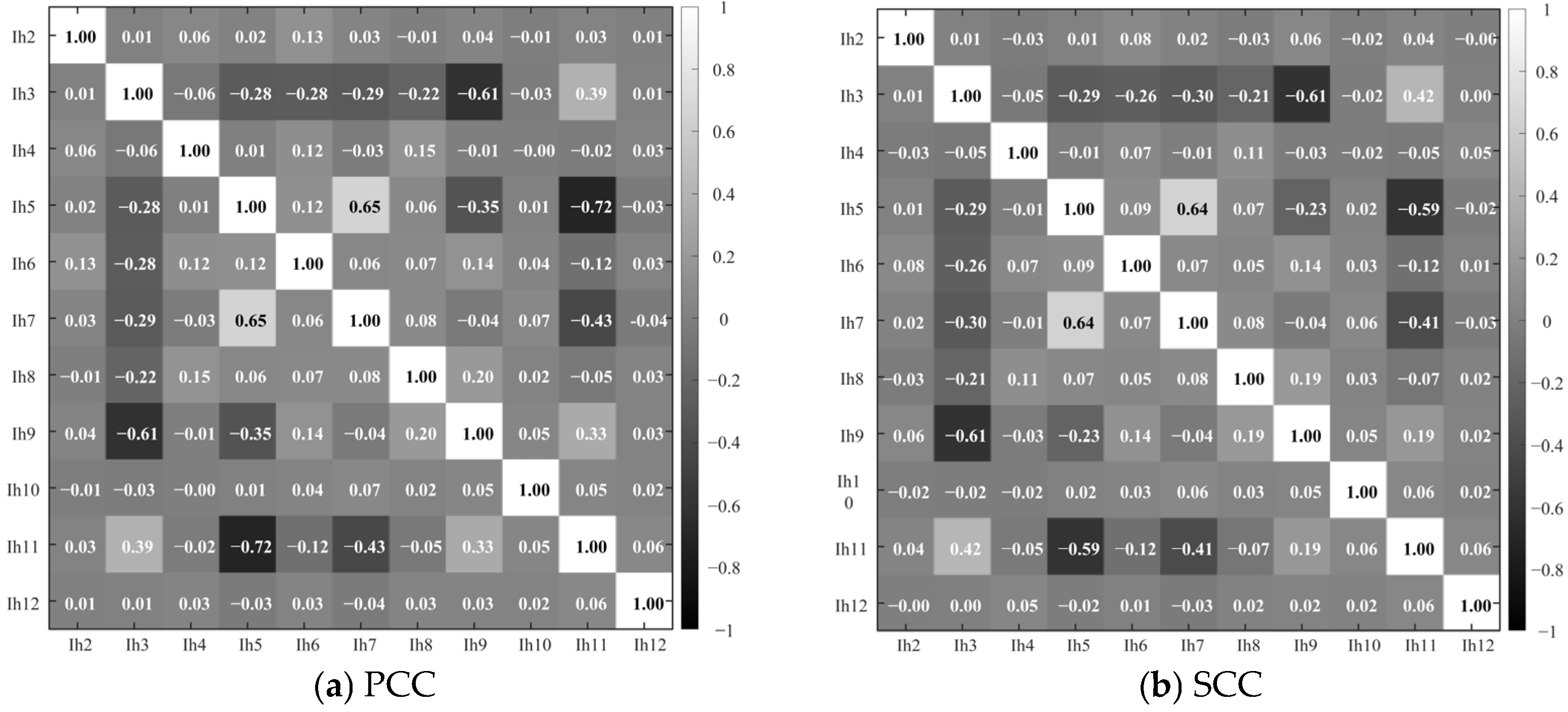
To investigate the coupling among different harmonics, this study utilizes harmonic monitoring data from a 500 kV substation. The Pearson Correlation Coefficient (PCC) and Spearman Correlation Coefficient (SCC) are computed among harmonic currents of various orders to evaluate their linear and monotonic correlations, respectively. A heatmap is then plotted, as shown in Figure 6, to visualize these relationships.
  • Pearson Correlation Coefficient (PCC)
ρ x , y = i = 1 n ( x i x ¯ ) ( y i y ¯ ) i = 1 n ( x i x ¯ ) 2 i = 1 n ( y i y ¯ ) 2
Here, x and y represent the sampled data of different harmonic current components, x ¯ and y ¯ denote their sample means, and n is the total number of observations. The PCC measures the linear correlation between the two variables, with values ranging from −1 to 1. It is used to evaluate the linear trend in the variation of harmonic currents.
  • Spearman Correlation Coefficient (SCC)
ρ s = i = 1 n ( R i R ¯ ) ( S i S ¯ ) i = 1 n ( R i R ¯ ) 2 i = 1 n ( S i S ¯ ) 2 = 1 6 d i 2 n ( n 2 1 )
Here, Ri and Si denote the rank values of the ith observation for variables x and y, respectively. R ¯ and S ¯ are the average ranks of x and y, and di = RiSi. The SCC is computed based on rank statistics and is used to evaluate the monotonic relationship between variables. It is suitable for analyzing nonlinear dependencies. Like PCC, SCC ranges from −1 to 1, making it useful for identifying potential nonlinear coupling characteristics among harmonic currents.
From the heatmaps, the following observations can be made: (1) There exists a certain degree of correlation among odd-order harmonic currents. This correlation mainly arises from their common origin—nonlinear loads in the power system—and the fact that their frequencies are all odd multiples of the fundamental frequency. (2) Even-order harmonic currents also exhibit some correlation, but it is relatively weaker. This is primarily due to the characteristics of the power system and the generation mechanisms of even harmonics. For example, even-order harmonics are typically negligible in a balanced three-phase system. (3) There is generally no significant correlation between odd- and even-order harmonic currents. This is because they are generated by different mechanisms, have distinct frequency characteristics, and may be influenced by different factors in the power system.
The correlation among harmonic currents may vary depending on system states, load characteristics, and operating conditions. Therefore, a detailed analysis tailored to specific scenarios is essential. To this end, the Single-Task Gaussian Process Regression (ST-GPR) model is extended to a Multi-Task Gaussian Process Regression (MT-GPR) model. By fully incorporating the interdependencies among harmonic currents in the modeling process, this approach not only significantly improves prediction accuracy but also enables the construction of a unified model that captures the joint behavior of multiple harmonic currents. The harmonic source modeling process based on MT-GPR is outlined as follows:
For homogeneous training sets X1 = ⋯ = Xt = X, assume that the function set F = {F1, F2, …, Ft} follows a Gaussian process, i.e., F(x) ~ GP (0, κ(x, x′)). Then, the multi-output covariance function κ(x, x′) ∈ ℝT×T is defined as follows:
κ x , x = k 11 ( x , x ) k 1 T ( x , x ) k T 1 ( x , x ) k T T ( x , x )
Here, x, x′ ∈ X, and ktt(x, x′) (1 ≤ t, t′ ≤ T) denotes the covariance between outputs Ft(x) and Ft(x).
Similar to standard GPR, for a given harmonic training set X ˜ = { X 1 , , X T } T and the corresponding output observations I = { I 1 , , I T } T , the posterior distribution of the predicted output at a test point x is defined as follows:
I | X ˜ , I , x ~ N I ¯ , c o v ( I )
where the predictive mean and variance are given by the following:
I ¯ = κ ( x , X ) [ κ ( X , X ) + Σ n E n ] 1 I
c o v ( I ¯ ) = κ ( x , x ) κ ( x , X ) [ κ ( X , X ) + Σ n E n ] 1 κ ( X , x )
Here, κ(X, X) ∈ ℝnT×nT, κ(X, x*) = (ktt(X, x*)) ∈ ℝnT×T, κ(x*, x*) = (ktt′(x*, x*))∈ℝT×T, and Σn∈ℝT×T is a diagonal matrix whose elements represent the observation noise variances for each task.
Similar to standard GPR, the hyperparameters in MT-GPR, including those in the kernel function {ktt′}1≤t,t′≤T and the noise covariance { σ n . t 2 }1≤tT, can be optimized by minimizing the objective in Equation (10).

3.3. Adaptive Kernel Function Design

In kernel functions, the length-scale parameter l determines the degree of smoothness in the input data. A smaller length scale makes the kernel more sensitive to variations in the input, allowing it to capture local features, while a larger length scale results in smoother responses, favoring the modeling of global trends. In multi-task learning, different tasks (i.e., harmonic currents of different orders) may exhibit the following differences:
  • Different feature scales—for instance, as demonstrated by the analysis in Figure 3, lower-order harmonic currents typically have larger magnitudes, while higher-order components are relatively smaller.
  • Different data distributions—harmonic currents of different orders may follow distinct statistical patterns.
To accommodate these differences, assigning an independent and learnable length-scale parameter li for each task enables the kernel to better capture task-specific feature scales, thereby improving the model’s flexibility and adaptability. The Matern kernel can well adapt to multimodal data and data with steep changes, making it particularly advantageous for handling complex datasets. Saws-tooth waveforms often feature steep edges and sharp changes. The Matern kernel can effectively handle these steep changes by modifying its function characteristics, without overfitting the data. In this work, we adopt the Matern kernel, which is defined as follows:
k ( i ) ( x , x ) = σ f 2 1 + 3 d ( x , x ) l i exp 3 d ( x , x ) l i
Here, σ f 2 denotes the signal variance, l is the length-scale parameter, and d ( x , x ) represents the Euclidean distance between inputs.
By combining task-specific length scales with a task relationship matrix, a multi-task kernel function is constructed as follows:
k ( ( x i , t i ) , ( x j , t j ) ) = A t i t j k ( t i ) ( x i , x j )
Here, t i and t j denote the task indices (i.e., the orders of harmonic currents), and A t i t j is the task relationship matrix that characterizes the correlation between tasks t i and t j .
Similar to standard GPR, the task-specific length scales and the task relationship matrix A are jointly optimized by minimizing the Negative Logarithmic Marginal Likelihood (NLML).
Self-adaptive kernel functions adjust their parameters dynamically through optimization algorithms during the training process, thereby better fitting the data. During training, the parameters of the kernel function are adjusted through optimization algorithms to minimize the error in model fitting to the training data.
  • Initial setting: During the definition of the model, initial parameters may be set to some predefined values.
  • Optimization process: Parameters are adjusted through optimization algorithms. Specifically, first, the optimization algorithm adjusts the parameters based on the loss function (such as negative log-likelihood). Next, parameter updates occur, and in each iteration, the optimization algorithm computes the gradient of the loss function with respect to the parameters and adjusts the parameters accordingly.
This ensures that the model is optimized gradually during training, thereby achieving better data fitting.

3.4. Adaptive Multi-Task Gaussian Process Regression for General Probabilistic Harmonic Modeling

The general probabilistic harmonic modeling method based on Adaptive Multi-Task Gaussian Process Regression (AMT-GPR) provides an efficient and robust solution for harmonic analysis by jointly modeling multiple harmonic signals and producing probabilistic predictions. Starting from the characteristics of harmonic signals, the method constructs a multi-task framework and employs an adaptive multi-output covariance function to dynamically capture the correlations among different harmonic current components, thereby modeling the complex harmonic relationships observed in real-world data. The specific procedure consists of the following steps:
  • Data Preparation: Preprocess the acquired harmonic signals, construct the multi-task output matrix, and partition the dataset into training and testing sets;
  • Model Design: Select a covariance function suitable for multi-task modeling and adopt the adaptive Matern kernel to capture the smoothness and periodic characteristics of the harmonic signals;
  • Hyperparameter Optimization: Optimize the task-specific length scales, covariance matrix parameters, and noise variances using maximum likelihood estimation or Bayesian optimization techniques;
  • Model Training: Compute the covariance matrix of the training set and derive the posterior distribution based on Equations (16) and (17) to obtain the predictive mean and variance;
  • Model Evaluation: Assess the prediction accuracy using test data, with performance metrics such as Mean Squared Error (MSE) and Mean Absolute Percentage Error (MAPE).

4. Case Study

4.1. Performance Analysis of the Improved Model

To investigate the impact of the proposed improvements—namely, the adaptive kernel function and multi-output regression—on model accuracy and training time, this study compares three approaches: Single-Task GPR (ST-GPR), Multi-Task GPR (MT-GPR), and the proposed Adaptive Multi-Task GPR (AMT-GPR). These models are used to estimate the third-, fifth-, seventh-, and ninth-order harmonic currents in a high-voltage substation. (Higher-order harmonics typically exhibit low amplitudes and high randomness, making them less relevant for harmonic analysis in practical engineering applications, where more attention is paid to lower-order harmonics with higher amplitudes.)
The input features are constructed using the fundamental voltage, fundamental current, and the 3rd-, 5th-, 7th-, 9th-, and 11th-order harmonic voltages of phase A, extracted via fast Fourier transform (FFT) from high-frequency sampled data. A total of 1440 samples are used, and the corresponding harmonic currents serve as the output variables. A randomly selected 70% of the dataset is used as the training set for model validation.
Taking the third, fifth, and seventh harmonic currents as examples, the prediction results of the models are shown in Figure 7. The yellow line represents the ground truth, while the other colored lines represent the predictions of the three models, with shaded areas indicating the 95% confidence intervals of each method. Additionally, the performance metrics of the models are summarized in Table 1.
The simulation results indicate that MT-GPR, by introducing joint modeling across multiple tasks, effectively leverages the correlations among different harmonic components and demonstrates clear advantages in handling multi-task harmonic prediction problems. Taking the 3rd- and 11th-order harmonic current predictions as examples, the MT-GPR model reduces the MPE, MAPE, and MSE of the third-order harmonic current by 0.61%, 0.84%, and 1.37, respectively, compared to the ST-GPR model. For the 11th-order harmonic current, the reductions are 19.94%, 4.67%, and 0.65, respectively.
In addition, the coverage probability (CP) generally exceeds 96%, and the average interval width (AIW) for the third-order harmonic current decreases significantly from 10.09 to 4.56. Moreover, the multi-task modeling framework reduces redundant computations, thereby improving training efficiency to some extent. Therefore, MT-GPR achieves notable improvements in prediction accuracy, uncertainty quantification, and computational efficiency.
However, in practical applications, different harmonic signals exhibit varying feature scales. For instance, lower-order harmonics with larger magnitudes (such as the 3rd, 5th, and 7th orders) tend to have larger feature scales, while higher-order harmonics with smaller magnitudes (such as the 9th and 11th orders) exhibit smaller feature scales. Although MT-GPR demonstrates advantages in multi-task harmonic modeling by exploiting inter-task correlations, it still falls short in accurately capturing complex harmonic characteristics and in quantifying prediction uncertainty. In contrast, the proposed Adaptive Multi-Task GPR (AMT-GPR) assigns independent and learnable length-scale parameters to each task, introducing an adaptive mechanism that improves the kernel optimization efficiency. This enables the model to capture task-specific feature scale differences more effectively. As a result, AMT-GPR achieves further improvements over MT-GPR: for the 3rd-order harmonic current, the MPE, MAPE, and MSE are reduced by 3.09%, 0.12%, and 0.21, respectively; for the 11th-order harmonic current, the reductions are 5.96%, 0.03%, and 0.08, respectively. The coverage probability (CP) remains consistently above 96%, and the AIW for the 11th-order harmonic current decreases from 3.15 to 1.61, indicating that the AMT-GPR model maintains reliable performance even under challenging conditions. Furthermore, detailed analysis reveals that higher-order harmonics, such as the 11th order, exhibit relatively larger prediction errors, with MPE and MAPE reaching 19.12% and 3.7%, respectively. This phenomenon can be attributed to two main factors: (1) The significantly lower magnitude of high-order harmonic currents leads to a reduced signal-to-noise ratio (SNR). (2) High-order harmonics often exhibit pronounced sawtooth-like waveform characteristics, increasing signal nonlinearity and posing greater challenges for accurate modeling.
Based on the result, higher-order harmonics, such as the eleventh harmonic, exhibit higher errors and smaller amplitudes. To address this imbalance, one can examine methods such as data augmentation or weighted loss functions and discuss their potential effects. Specifically, the use of a weighted loss function can improve model performance by adjusting the loss weights to make the model more sensitive to errors in the high-frequency components. The advantage of this approach is that by adjusting the loss weights, the model becomes more focused on errors in the high-frequency components, thereby improving the fitting accuracy of these components. However, this method also has a disadvantage in that it increases the training complexity, requiring additional computational resources for both the calculation and application of the weights.
The simulation results demonstrate that compared with ST-GPR and MT-GPR, the proposed AMT-GPR model achieves significant improvements in prediction accuracy, uncertainty quantification, and computational efficiency, thereby validating the effectiveness of the proposed modeling approach and offering a practical solution for engineering applications.
The AMT-GPR model is suitable for real-time applications. Essentially, it is a machine learning algorithm. Although the training process is time-consuming, once the model is trained and deployed, the actual prediction speed is very fast. However, when the system undergoes significant changes (e.g., sudden changes in the harmonic spectrum), the previously trained model may no longer be applicable. In such cases, retraining the model is necessary to ensure accuracy. While retraining may take some additional time, this sacrifice is necessary to guarantee the model’s accuracy and reliability.
Compared to real-time simulation or analytical solving methods, machine learning algorithms clearly have distinct advantages in terms of usage. Specifically, when the system state is relatively stable, the AMT-GPR model can achieve a balance between speed and accuracy. However, since the system state is unlikely to remain unchanged, when the system changes, the previously trained model may result in decreased accuracy. In such cases, if adjustments or retraining are made, although some real-time performance may be sacrificed, the model’s accuracy can be significantly improved.
In summary, the AMT-GPR model can effectively balance speed and accuracy when the system state remains unchanged. However, when the system state changes, retraining is necessary to ensure high accuracy, despite the additional time delay. This trade-off is reasonable in practical applications.

4.2. Comparison with Other Modeling Methods

Based on the same set of measured data, the proposed AMT-GPR model is further compared with other existing harmonic source modeling methods reported in the literature. These methods include the Radial Basis Function Neural Network (RBF) proposed in [31], the Least Squares Support Vector Machine (LS-SVM) approach in [35], and the Long Short-Term Memory (LSTM) neural network method in [36], which incorporates temporal sequence characteristics of the data. All these approaches fall under the category of data-driven machine learning models.
A randomly selected 70% of the dataset is used as the training set for each model. The prediction results are illustrated in Figure 8, and the performance metrics are summarized in Table 2. Since the aforementioned comparison models do not provide uncertainty quantification (e.g., prediction intervals), the evaluation focuses solely on MPE, MAPE, and MSE metrics.
The results demonstrate that AMT-GPR significantly outperforms the other methods. Taking the third-order harmonic as an example, its MPE, MAPE, and MSE reach 3.46%, 0.49%, and 0.87, respectively. Compared to the best-performing alternative model, LSTM, the MAPE and MSE of AMT-GPR are reduced by 0.49% and 0.13%, respectively. Compared to the worst-performing method, LS-SVM, the reductions are 2.82%, 0.51%, and 0.89, respectively, highlighting the superior performance of AMT-GPR in point estimation tasks. Therefore, its predictive mean can be directly adopted as the final output.
In addition, by analyzing Figure 8 and Table 2 together, it is evident that the LS-SVM model exhibits relatively poor fitting accuracy. For the third-order harmonic current, its MPE, MAPE, and MSE are as high as 6.28%, 1.00%, and 1.76, respectively, with the predicted curve showing noticeable deviations from the measured values in certain cases. This result suggests that not all data-driven machine learning models perform well in fitting tasks; their effectiveness also depends on the complexity of the problem, the size of the training dataset, and data quality. For instance, LS-SVM may lack sufficient fitting capacity when dealing with harmonic source characteristics involving strong nonlinearity and multivariate coupling. In addition, limited data samples may prevent the model from adequately learning complex nonlinear features. Therefore, in engineering practice, it is essential to conduct multidimensional analyses based on problem characteristics and data properties to optimize model performance.

4.3. Analysis of the Impact of Data Conditions on Model Performance

To further analyze the impact of data conditions on model performance, 10% of the samples are randomly selected as the training set in this section. Based on the measured data from a high-voltage substation, four data-driven modeling methods—namely, LS-SVM, RBF, LSTM, and the proposed AMT-GPR, as described in Section B—are used to establish harmonic source models. The corresponding prediction results and performance metrics are presented in Figure 9 and Table 3.
The results show that AMT-GPR significantly outperforms the other methods. Taking the third-order harmonic as an example, its MPE, MAPE, and MSE reach 3.77%, 0.59%, and 1.02, respectively. Compared to the best-performing alternative model (LSTM), the MPE, MAPE, and MSE are reduced by 1.33%, 0.19%, and 0.39, respectively. Compared to the worst-performing method (LS-SVM), the reductions are 8.24%, 2.49%, and 3.84, respectively.
A comparison between Table 2 and Table 3 reveals that when the size of the training dataset is small, the prediction error of the models generally increases significantly—particularly for LS-SVM. Further analysis shows that AMT-GPR exhibits low sensitivity to training data size and demonstrates strong robustness. This characteristic highlights its superiority under small-sample conditions and enhances its practical value in engineering applications. The main reasons are as follows:
  • Gaussian Process Regression (GPR) is a Bayesian non-parametric model that, unlike traditional machine learning methods such as neural networks, does not require a large amount of data to optimize parameters. Instead, GPR models the relationships between input data points through a kernel function. As a result, its predictions rely on data distribution rather than parameter fitting, allowing for reasonable prediction performance even with limited data.
  • AMT-GPR is a multi-task learning method that models inter-task relationships by sharing the kernel function. This enables information sharing across tasks, so that even when the data for a single task is sparse, the model can leverage data from other tasks for auxiliary learning, thereby improving robustness.
  • The introduction of an adaptive kernel function allows the model to maintain stable performance under varying data sizes, reducing its sensitivity to data quantity. The adaptive mechanism enables the model to reduce complexity and avoid overfitting with limited data, while enhancing accuracy and generalization capability when more data are available.
In contrast, other methods such as LS-SVM and RBF are more sensitive to dataset size, which is mainly reflected in their higher risk of overfitting when data is insufficient and degraded performance when the data distribution changes.
In summary, the influence of sample size on model prediction error is multifaceted:
  • From a statistical perspective, as the number of harmonic samples increases, the statistical characteristics of the sample (e.g., mean, variance) more closely approximate those of the population. This implies that larger datasets yield estimates that are closer to the true values, thereby reducing prediction errors;
  • From the perspective of model training, expanding the dataset enhances the model’s capacity to capture harmonic characteristics, thereby improving prediction accuracy;
  • In terms of generalization, increasing the sample size helps to mitigate overfitting and improves the model’s generalization ability.
Therefore, in practical engineering applications, constructing a sufficiently large and representative training dataset is a critical factor in ensuring high prediction performance.

4.4. Probabilistic Modeling of Harmonic Sources

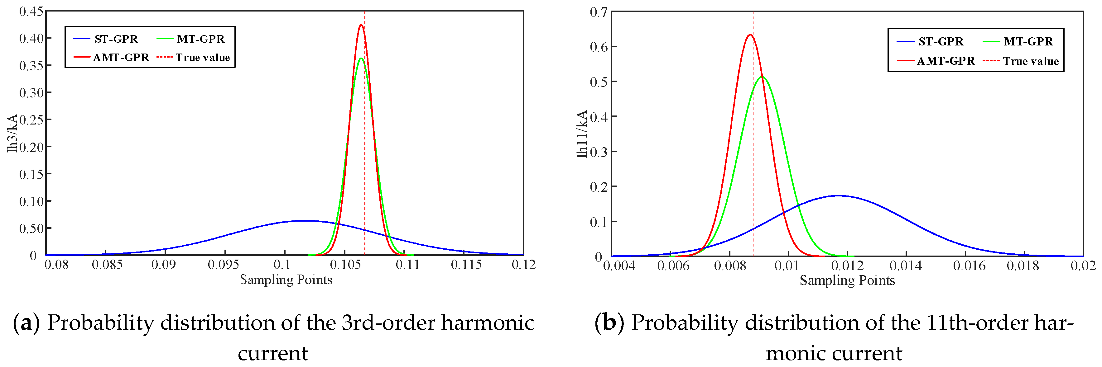
In this section, the model prediction results at a representative time instant are selected, and Gaussian distributions of each harmonic current are constructed using the predicted mean and standard deviation as parameters. This provides an intuitive comparison of the predictive performance of each model, as shown in Table 4.
Figure 10 illustrates the probability distributions of the predicted 3rd- and 11th-order harmonic currents at a specific time instant. By comparing the results of the ST-GPR, MT-GPR, and AMT-GPR models, it is observed that the AMT-GPR distribution exhibits a sharper peak and narrower tails, indicating both higher prediction accuracy and lower uncertainty. In contrast, the distributions produced by ST-GPR and MT-GPR are more dispersed, with lower peaks and wider tails. Among them, ST-GPR performs the worst, reflecting lower prediction accuracy and higher uncertainty. This comparison further validates the significant advantages of AMT-GPR in terms of prediction precision and robustness.

5. Conclusions

This paper proposes a general probabilistic harmonic modeling method based on Adaptive Multi-Task Gaussian Process Regression (AMT-GPR) to address the modeling of aggregated load harmonics in high-voltage substations. By integrating an adaptive kernel function with a multi-task learning framework, AMT-GPR effectively captures the correlations among different harmonic components and adaptively adjusts to their varying feature scales. This significantly enhances both prediction accuracy and model robustness. The main conclusions are as follows:
  • Harmonic Characteristic Analysis: Based on measured data from a high-voltage substation, the time-varying characteristics of harmonics generated by aggregated loads are analyzed. The results reveal a strong correlation between harmonic currents and system load variations, providing a solid data foundation for harmonic modeling.
  • Model Design: The proposed AMT-GPR method assigns independent and trainable length-scale parameters to each harmonic task, enabling adaptive feature scale learning. This design substantially improves model flexibility and adaptability across different harmonic orders.
  • Performance Validation: Through comparative experiments with ST-GPR, MT-GPR, and other data-driven approaches (including LS-SVM, RBF, and LSTM), AMT-GPR demonstrates superior performance in prediction accuracy, uncertainty quantification, and computational efficiency. The results show that AMT-GPR performs well for both low- and high-order harmonics and exhibits strong robustness under small training datasets.
  • Probabilistic Modeling: Based on the AMT-GPR prediction results, Gaussian probability distributions of harmonic currents are constructed, providing a reliable theoretical foundation for subsequent probabilistic harmonic power flow analysis.
Harmonic power flow analysis requires modeling harmonic sources in the power grid. AMT-GPR serves as a harmonic source modeling method that can replace previous approaches. Further developing probabilistic harmonic power flow calculation tools based on AMT-GPR represents one of the future research directions.

Author Contributions

Conceptualization, J.Z.; methodology, J.Z. and K.S.; software, J.D. and Y.W.; validation, K.S.; resources, K.S.; writing—original draft, J.Z. and K.S.; writing—review and editing, J.Z.; visualization, J.D.; supervision, Y.W. All authors have read and agreed to the published version of the manuscript.

Funding

This research received no external funding.

Data Availability Statement

Data is unavailable due to privacy or ethical restriction.

Conflicts of Interest

Author Kun Song was employed by Chengdu Electric Power Supply Company, State Grid Sichuan Power Supply Company. The remaining authors declare that the research was conducted in the absence of any commercial or financial relationships that could be construed as a potential conflict of interest.

References

  1. Shao, Z.; Xu, H.; Xiao, S.; Wu, G.; Zhang, Y. Harmonic problems in a new energy power grid. Power Syst. Prot. Control 2021, 49, 178–187. [Google Scholar] [CrossRef]
  2. Valavi, M.; Devillers, E.; Besnerais, J.L.; Nysveen, A.; Nilsen, R. Influence of converter topology and carrier frequency on airgap field harmonics, magnetic forces, and vibrations in converter-fed hydropower generator. IEEE Trans. Ind. Appl. 2018, 54, 2202–2214. [Google Scholar] [CrossRef]
  3. Domínguez-Crespo, M.A.; Rodríguez, E.; Torres-Huerta, A.M.; Soni-Castro, I.J.; Brachetti-Sibaja, S.B.; Narro-García, R.; López-Oyama, A.B. Production of BN nanostructures by pulsed laser ablation in liquids: Influence of the applied Nd: YAG harmonics on the structural, optical and photoluminescence properties. Ceram. Int. 2020, 46, 21667–21680. [Google Scholar] [CrossRef]
  4. Zhang, W.; Xiong, Y.; Li, C.; Yao, W.; Wen, J.; Gao, D. Continuous commutation failure suppression and coordinated recovery of multi-infeed DC system based on improved VDCOL. Power Syst. Prot. Control 2020, 48, 63–72. [Google Scholar] [CrossRef]
  5. Chen, L.; He, H.; Wang, L.; Chen, H. Fault isolation method of a hybrid HVDC system based on the coordination of a fault current limiter and a DC circuit breaker. Power Syst. Prot. Control 2020, 48, 119–127. [Google Scholar] [CrossRef]
  6. Hiyama, T.; Hammam, M.S.A.A.; Ortmeyer, T.H. Distribution system modeling with distributed harmonic sources. IEEE Trans. Power Deliv. 1992, 4, 1297–1304. [Google Scholar] [CrossRef]
  7. Salles, D.; Jiang, C.; Xu, W.; Freitas, W.; Mazin, H.E. Assessing the collective harmonic impact of modern residential loads—Part I: Methodology. IEEE Trans. Power Deliv. 2012, 27, 1937–1946. [Google Scholar] [CrossRef]
  8. Jiang, C.; Salles, D.; Xu, W.; Freitas, W. Assessing the collective harmonic impact of modern residential loads—Part II: Applications. IEEE Trans. Power Deliv. 2012, 27, 1937–1946. [Google Scholar] [CrossRef]
  9. Thunberg, E.; Soder, L. Norton approach to distribution network modeling for harmonic studies. IEEE Trans. Power Deliv. 1999, 14, 272–277. [Google Scholar] [CrossRef]
  10. Fauri, M. Harmonic modelling of non-linear load by means of crossed frequency admittance matrix. IEEE Trans. Power Syst. 1997, 12, 1632–1638. [Google Scholar] [CrossRef]
  11. Sun, Y.; Zhang, G.; Xu, W.; Mayordomo, J.G. A harmonically coupled admittance matrix model for AC/DC converters. IEEE Trans. Power Syst. 2007, 22, 1574–1582. [Google Scholar] [CrossRef]
  12. Sun, Y.; Li, J.; Yin, Z.; Wang, G. A frequency domain harmonic model for uncontrolled rectifier in AC/DC/AC converter. Proc. CSEE 2015, 35, 5483–5491. [Google Scholar] [CrossRef]
  13. Sun, Y.; Liu, F.; Li, J.; Kun, Z. Unified harmonic models and operational mode determination for the three-phase uncontrolled voltage source converters. Proc. CSEE 2016, 36, 3413–3421+3360. [Google Scholar] [CrossRef]
  14. Sun, Y.; Zhang, L.; Xie, X.; Feng, Z.; Wang, S. The collective harmonic evaluation of residential load based on the harmonic coupling dominant component model. Proc. CSEE 2019, 39, 4775–4785+4979. [Google Scholar] [CrossRef]
  15. Xie, X.; Sun, Y.; Zhang, L.; He, J.; Zhang, Y. Self-adaptive harmonic modeling of the residential nonlinear load. Proc. CSEE 2020, 40, 2479–2489. [Google Scholar] [CrossRef]
  16. Liao, Y.; Hu, J.; Zhang, H. Time-varying parameter model of AC electrical arc furnace for power quality predictions and analysis. Electr. Eng. 2016, 17, 41–46. [Google Scholar]
  17. Wang, J.; Shu, H.; Lin, M.; Xueyun, C. Modeling and simulation of AC arc furnace for dynamic power quality studies. Trans. China Electrotech. Soc. 2003, 18, 53–58. [Google Scholar] [CrossRef]
  18. King, P.E.; Ochs, T.L.; Hartman, A.D. Chaotic response in electric arc furnaces. J. Appl. Phys. 1994, 76, 2059–2065. [Google Scholar] [CrossRef]
  19. Wang, Y.; Jiang, J. A novel chaotic model of AC electric arc furnace for power quality study. In Proceedings of the 2007 International Conference on Electrical Machines and Systems (ICEMS), Seoul, Republic of Korea, 8–11 October 2007; pp. 106–110. [Google Scholar]
  20. Lin, C.; Zhang, Y.; Shao, Z.; Lin, C.; Zhang, Y. An ultra-high-power electric arc furnace model for low-frequency non-stationary inter-harmonics studies. Electr. Power 2020, 53, 1–8. [Google Scholar]
  21. Nian, H.; Zhou, Q.; Wu, C.; Zhu, Q. The modeling and characteristic analysis of harmonic current of DFIG based wind turbine in grid-connected mode. Proc. CSEE 2019, 39, 5037–5048+5285. [Google Scholar] [CrossRef]
  22. Zhang, B. Research on Harmonic Dynamic Model and Resonance Analysis of Wind Parks. Ph.D. Thesis, Shandong University, Jinan, China, 2019. [Google Scholar]
  23. Tao, S.; Zhu, X.; Chen, H.; Xu, Y. Dead-time coupling harmonic source modeling of grid-connected Inverter. Proc. CSEE 2024, 1–14. [Google Scholar]
  24. Che, Q.; Yang, H. Assessing the harmonic emission level based on robust regression method. Proc. CSEE 2004, 24, 43–46+53. [Google Scholar]
  25. Ortega, J.M.M.; Exposito, A.G.; Garcia, A.L.T.; Payan, M.B. A state estimation approach to harmonic polluting load characterization in distribution systems. IEEE Trans. Power Syst. 2005, 20, 765–772. [Google Scholar]
  26. Huang, S.; Xu, Y. Assessing harmonic impedance and the harmonic emission level based on partial least-squares regression method. Proc. CSEE 2007, 27, 93–97. [Google Scholar]
  27. Feng, F.; Xie, X. Assessment of network harmonic emission level via enhanced partial least-squares regression method. Metrol. Meas. Tech. 2014, 41, 33–35. [Google Scholar]
  28. Hua, H.C.; Jia, X.F.; An, H.Q.; Zhang, S.G. Determining harmonic contributions based on complex least squares method. Proc. CSEE 2013, 33, 149–155. [Google Scholar] [CrossRef]
  29. Yongle, A.; Yudong, W.; Jingjing, D.; Wang, W. A method for assessing harmonic emission level based on robust regression of LTS initial value. Power Syst. Prot. Control 2015, 43, 99–105. [Google Scholar]
  30. Moreno, M.A.; Usaola, J. A new balanced harmonic load flow including nonlinear loads modeled with RBF networks. IEEE Trans. Power Deliv. 2004, 19, 686–693. [Google Scholar] [CrossRef]
  31. Yong, Z.; Haozhong, C.; Naicheng, G. Generalized growing and pruning RBF neural network based harmonic source modeling. Proc. CSEE 2005, 25, 42–46. [Google Scholar]
  32. Maciej, K.; Dariusz, G. Application of shallow neural networks in electric arc furnace modeling. IEEE Trans. Ind. Appl. 2022, 58, 6814–6823. [Google Scholar] [CrossRef]
  33. Xie, K.; Yang, H.; Zhang, Y. Harmonic source modeling based on generalized regression neural network. Adv. Technol. Electr. Eng. Energy 2012, 31, 64–67. [Google Scholar]
  34. Zhang, Y.; Ou, J.; Chen, S.; Jie, K.; Liu, S. A data-driven harmonic source modeling method based on joint time-frequency features extraction. Proc. CSEE 2025, 1–14. [Google Scholar]
  35. Lianqing, Z.; Ping, W.; Xiaolong, L. Application of least squares support vector machine to harmonic sources modeling based on genetic algorithm. Power Syst. Prot. Control 2011, 39, 52–56. [Google Scholar]
  36. Yang, P.; Wang, X.; Zhao, X. Research on harmonic prediction of the grid-connected photovoltaic system based on deep learning. Power Syst. Clean Energy 2022, 38, 71–80. [Google Scholar]
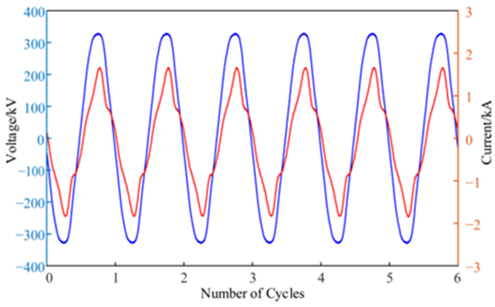
Figure 1. Measured voltage and current waveforms in high-voltage substation.
Energies 18 04670 g001
Figure 2. Residual plots of denoised voltage and current waveforms.
Energies 18 04670 g002
Figure 3. Variation of harmonic characteristics of aggregated loads in a high-voltage substation.
Energies 18 04670 g003
Figure 4. Harmonic current profiles of each order on two consecutive days at the same substation.
Energies 18 04670 g004
Figure 5. The statistical characteristics of the 3rd harmonic current.
Energies 18 04670 g005
Figure 6. Heatmaps of PCC and SCC among harmonic currents of different orders.
Energies 18 04670 g006
Figure 7. Model prediction results for the 3rd-, 5th-, and 7th-order harmonic currents.
Energies 18 04670 g007
Figure 8. Model prediction results for the 3rd, 5th, and 7th-order harmonic currents.
Energies 18 04670 g008
Figure 9. Model prediction results for the 3rd, 5th, and 7th-order harmonic currents.
Energies 18 04670 g009
Figure 10. Probability distributions of harmonic currents at a specific time instant (3rd and 11th orders).
Energies 18 04670 g010
Table 1. Performance evaluation results of the above models.
ModelHarmonic OrderMPE (%)MAPE (%)MSECP (%)AIWTraining Time (s)
ST-GPR3th7.161.452.4596.010.0921.7
5th11.351.081.8687.47.3222.6
7th13.982.651.1288.73.8219.2
9th14.291.830.6199.43.5025.6
11th45.028.401.3399.26.7126.5
MT-GPR3th6.550.611.0896.24.5618.7
5th7.830.460.8596.13.25
7th8.741.400.5794.12.18
9th5.941.200.4096.01.62
11th25.083.730.6896.13.15
AMT-GPR3th3.460.490.8796.53.8816.2
5th1.750.400.6697.12.94
7th5.581.200.4896.62.08
9th5.661.160.3895.81.57
11th19.123.700.6095.81.61
Table 2. Performance evaluation results of the models (70% training set).
ModelHarmonic OrderMPE (%)MAPE (%)MSE
LS-SVM3th6.281.001.76
5th5.680.691.18
7th9.721.580.64
RBF3th4.010.731.54
5th2.360.460.81
7th6.631.300.54
LSTM3th3.950.621.06
5th2.640.400.67
7th6.311.200.49
AMT-GPR3th3.460.490.87
5th1.750.400.66
7th5.581.200.48
Table 3. Performance evaluation results of the models (10% training set).
ModelHarmonic OrderMPE (%)MAPE (%)MSE
LS-SVM3th12.013.084.86
5th7.571.212.11
7th16.862.931.25
RBF3th5.361.412.35
5th7.380.981.72
7th13.892.611.08
LSTM3th5.100.781.38
5th6.450.571.03
7th8.431.540.63
AMT-GPR3th3.770.591.02
5th5.740.440.85
7th6.541.320.54
Table 4. Gaussian distributions of harmonic current outputs from different models at time t.
ModelST-GPRMT-GPRAMT-GPRTrue Value
Ih3N (1.017 × 10⁻¹, 6.3 × 10⁻³)N (1.064 × 10⁻¹, 1.1 × 10⁻³)N (1.064 × 10⁻¹, 9.4 × 10⁻⁴)1.067 × 10⁻¹
Ih5N (1.391 × 10⁻¹, 4.7 × 10⁻³)N (1.415 × 10⁻¹, 7.7 × 10⁻⁴)N (1.414 × 10⁻¹, 7.1 × 10⁻⁴)1.412 × 10⁻¹
Ih7N (3.32 × 10⁻², 2.0 × 10⁻³)N (3.54 × 10⁻², 5.29 × 10⁻⁴)N (3.54 × 10⁻², 5.04 × 10⁻⁴)3.55 × 10⁻²
Ih9N (2.58 × 10⁻², 1.9 × 10⁻³)N (2.60 × 10⁻², 4.05 × 10⁻⁴)N (2.58 × 10⁻², 3.91 × 10⁻⁴)2.65 × 10⁻²
Ih11N (1.17 × 10⁻², 2.3 × 10⁻³)N (9.10 × 10⁻³, 7.78 × 10⁻⁴)N (8.70 × 10⁻⁴, 6.30 × 10⁻⁴)8.80 × 10⁻³
Disclaimer/Publisher’s Note: The statements, opinions and data contained in all publications are solely those of the individual author(s) and contributor(s) and not of MDPI and/or the editor(s). MDPI and/or the editor(s) disclaim responsibility for any injury to people or property resulting from any ideas, methods, instructions or products referred to in the content.