Abstract
Batteries are ubiquitous, with their presence ranging from electric vehicles to portable electronics. Research focused on increasing average voltage, improving stability, and extending cycle longevity of batteries is pivotal for the advancement of battery technology. These advancements can be accelerated through research into battery chemistries. The traditional approach, which examines each material combination individually, poses significant challenges in terms of resources and financial investment. Physics-based simulations, while detailed, are both time-consuming and resource-intensive. Researchers aim to mitigate these concerns by employing Machine Learning (ML) techniques. In this study, we propose a Transformer-based deep learning model for predicting the average voltage of battery electrodes. Transformers, known for their ability to capture complex dependencies and relationships, are adapted here for tabular data and regression tasks. The model was trained on data from the Materials Project database. The results demonstrated strong predictive performance, with lower mean absolute error (MAE) and mean squared error (MSE), and higher R2 values, indicating high accuracy in voltage prediction. Additionally, we conducted detailed per-ion performance analysis across ten working ions and apply sample-wise loss weighting to address data imbalance, significantly improving accuracy on rare-ion systems (e.g., Rb and Y) while preserving overall performance. Furthermore, we performed SHAP-based feature attribution to interpret model predictions, revealing that gravimetric energy and capacity dominate prediction influence, with architecture-specific differences in learned feature importance. This work highlights the potential of Transformer architectures in accelerating the discovery of advanced materials for sustainable energy storage.
1. Introduction
To address the need for battery-powered electric vehicles and large-scale energy storage systems, it is necessary to identify promising battery electrode materials for rechargeable batteries [1]. The intermittent nature of sustainable energy resources further underscores the need for efficient and reliable storage solutions [2]. Historically, the lack of effective secondary batteries hindered the development of technologies such as electric vehicles and wireless communications, a challenge largely rooted in the limitations of electrode materials, electrolytes, and interface control [3]. For instance, lithium (Li) is a promising element for energy storage due to its high energy density, but its extraction and processing are costly and environmentally intensive [4]. Similarly, cobalt, an indispensable cathode material, is rare, expensive, and associated with geopolitical and ethical concerns [5]. These challenges have prompted researchers to explore alternative electrode materials and new battery chemistries [6,7].
The energy storage capacity of a battery is determined by both its voltage and the materials used in its electrodes [3]. A higher open-circuit voltage in the positive electrode is critical for maximizing energy density, as the energy density is directly proportional to the potential difference. However, achieving a high open-circuit voltage requires careful consideration of the stability of electrolytes and the properties of electrode materials to prevent degradation and ensure long-term performance. Moreover, advancing battery technologies requires balancing energy performance with factors such as material abundance, sustainability, and cost.
There are two possible approaches to determining the voltage of battery electrodes: the traditional experimental approach and the physics-based computational method. The traditional trial-and-error experimentation and theoretical calculations are both time-consuming and resource-intensive for identifying suitable electrode materials [8,9]. While computational methods like density functional theory (DFT) can calculate the potential of electrode materials, they are limited to simpler chemical systems, are computationally expensive, and remain impractical for exploring the vast chemical space of electrode materials [9].
ML provides a faster alternative, but several challenges remain. Many existing voltage prediction models underperform on underrepresented ions due to dataset imbalance, often rely on large datasets not available for less-studied chemistries (e.g., Mg, Zn, Al), and lack interpretability, making it difficult to validate predictions in a scientific context [8,10,11]. In addition, models such as support vector machines (SVMs), kernel ridge regression (KRR), and conventional deep neural networks (DNNs) perform well within specific chemistries but transfer poorly across systems [12,13,14]. These limitations highlight the need for scalable and interpretable architectures that maintain accuracy across diverse chemistries, particularly for rare ions such as Rb and Y.
Even with progress in experiments and simulations, discovering new battery electrode materials remains challenging. Lab experiments take a lot of time and resources, while computational methods like DFT are costly and cannot easily scale to large chemical spaces. ML offers speed and flexibility but is constrained by the limitations summarized above. Addressing these issues requires models that are data-efficient, transferable across chemistries, and interpretable enough to provide meaningful insights for materials discovery.
Our work makes the following contributions:
- i
- We develop a scalable deep learning pipeline for voltage prediction from structured material data, avoiding complex simulations. Within this pipeline, we implement and evaluate four Transformer-based models—Base Transformer, Transformer + Feedforward Neural Network (FFNN), Transformer + Gated Recurrent Unit (GRU), and Transformer + Long Short-Term Memory (LSTM)—demonstrating how combining attention with dense or recurrent layers enhances regression accuracy.
- ii
- We perform a comparative analysis of these models using standard metrics such as MAE, MSE, and . Each metric captures different aspects of regression performance—robustness to outliers, sensitivity to large deviations, and variance explained—providing a comprehensive assessment.
- iii
- We conduct a detailed per-ion performance analysis using MAE, MSE, and metrics across ten working ions, including both abundant (e.g., Li and Na) and underrepresented species (e.g., Rb and Y). This highlights variability in prediction accuracy due to class imbalance. To mitigate this, we apply sample-wise loss weighting, which significantly improves accuracy on rare ions (e.g., Rb improves from 0.8036 to 0.9832 in the FFNN model) while maintaining or enhancing overall metrics. Even simpler architectures like the Base Transformer benefit from better generalization, showing that loss weighting promotes fairness without compromising performance.
- iv
- We perform SHAP-based feature attribution to interpret model predictions. Gravimetric energy and capacity consistently emerge as the most influential features across most models. The Transformer + GRU model uniquely emphasizes site-specific magnetic moments, revealing how different architectures internalize and prioritize physical descriptors.
- v
- We extend interpretability beyond global feature importance by conducting local SHAP analyses on representative cases (best, median, and worst predictions) for the best-performing model. This provides sample-level insights into how the same features can drive both highly accurate predictions and large errors, enabling more trustworthy model evaluation.
- vi
- We enable fast, scalable screening of candidate battery electrode materials based on predicted voltage. This reduces reliance on costly, time-intensive DFT calculations and accelerates discovery in battery materials research.
This paper is structured as follows: Section 1 provides a brief introduction on the purpose of this study. Section 2 reviews related work and highlights the distinctions of our approach. Section 3 describes the methods used in this research, including data preprocessing, the detailed architecture of the proposed Transformer models, evaluation metrics such as MAE, MSE, and R2, and the composite loss function and implementation details. Section 4 presents the results and discussion, including performance comparisons of the models, training and validation loss plots, and residual error analysis. We further assess reliability through bootstrap-based uncertainty estimation, analyze per-ion performance with and without sample-wise loss weighting, and investigate feature importance using SHAP for both global and local interpretability. Finally, Section 5 concludes the paper by summarizing the key findings, discussing limitations, and highlighting directions for future research.
2. Background and Related Work
ML has emerged as an effective tool for accelerating battery materials discovery [10,15,16]. Numerous ML algorithms have been developed to predict the voltage of battery electrodes. Joshi et al. [12] trained DNNs, SVMs, and KRR models on Materials Project data, achieving voltage predictions for thousands of Na-ion and K-ion battery materials. Louis et al. [13] developed graph neural networks (GNNs) that improved generalization between Li-ion and Na-ion systems. In contrast, Babar et al. [17] used Bayesian regression with van der Waals corrections to model lithium–graphite systems. Similarly, Allam et al. [18] applied ML, trained on DFT-calculated electronic and structural features, to accelerate redox potential prediction.
These models typically rely on access to large and often multiple datasets. This poses a challenge for chemistries such as Mg, Zn, or Al, where data availability is limited. Ling [10] discusses this issue in the context of battery informatics. Zhang et al. [14] proposed a DNN model tailored to small datasets, incorporating transfer learning and identifying atomic covalent radius as a key feature for voltage prediction. Hossain et al. [19] developed a DNN to predict the average voltage of alkali metal-ion battery materials using features from the Materials Project, achieving a mean absolute error (MAE) of 0.069 V. While accurate, their work focused on conventional DNN architectures and did not explore alternative modeling approaches.
Beyond voltage prediction, ML has also been applied to the prediction of battery cycle life, capacity, and degradation [20,21,22]. Tao et al. [23] developed an adaptive ML framework to predict battery lifetime under different operating conditions. The framework uses interpretable feature engineering and correlation alignment (CORAL) to correct feature divergence between charging regimes. It achieves high early-cycle prediction accuracy with minimal input features. Jiang et al. [24] introduced a rapid and data-efficient model for lithium-ion battery lifetime prediction by combining a hierarchical Bayesian model (HBM) with a minimax probability machine. The standout feature of their method is its ability to predict battery cycle life with high accuracy after just three initial experimental cycles, dramatically reducing both testing time and resource use. Liu et al. [25] proposed an interpretable ML framework to predict multiple battery capacity types at the early production stage. The framework considers how key coating parameters—mass, thickness, and porosity—influence capacity. It also captures how these parameters interact with each other. Zhang et al. [26] developed BatLiNet, a deep learning framework that predicts battery lifetime under diverse ageing conditions by integrating single-cell and inter-cell learning to capture both individual degradation patterns and relative ageing behaviors. Tang et al. [27] present a physics-informed method for battery degradation prediction that integrates domain knowledge into ML. This method uses data from only a single present cycle to predict constant-current voltage–capacity curves for hundreds of future cycles. In doing so, it forecasts long-term battery degradation. Xia et al. [11] applied the SHAP interpretation method to ML for predicting battery health states from impedance spectra, identifying the frequency points most strongly associated with ageing, which allows the model to focus on a targeted frequency range of the spectrum for more accurate predictions.
In addition to these models, Transformer-based architectures have also been utilized for estimating battery state-of-charge (SOC) and state-of-health (SOH) [28]. Huang et al. proposed a multi-scale decomposition and fusion neural framework for SOH estimation that demonstrates strong cross-chemistry generalizability. The framework employs short-term charging curves combined with multi-scale decomposition and feature fusion, and was validated on 145 batteries across six chemistries and 14 operating conditions, demonstrating high accuracy and robustness [29]. Jia et al. proposed a hybrid bidirectional gated recurrent unit (BiGRU)–Transformer to accurately predict battery SOH. An indirect health indicator was constructed from discharge voltage curves using the time interval at equal voltage difference (TIEDVD) method. The model was trained and tested on the NASA PCoE dataset with three lithium-ion cells and achieved strong performance with a root mean square error of 0.00243 and a mean absolute percentage error of 0.19% [30]. Shi et al. proposed a CNN–Transformer model for estimating lithium-ion battery degradation. The model was trained and validated on charge–discharge data from 124 commercial /graphite cells (A123 APR18650M1A, 1.1 Ah) and achieved capacity prediction errors of less than 3% for most batteries [31].
Motivated by the efficient parallelism of attention-based Transformers, we propose a model for predicting the average voltage of battery electrodes, where the attention mechanism captures complex dependencies in the data. Such models have been widely used in natural language processing. We apply them here to structured battery data. We also explore hybrid models that combine Transformers with FFNN, GRU, or LSTM layers. Our goal is to evaluate the performance of Transformer-based models in predicting average voltage. We use data for ten metal-ion systems, including both common ions (Li, Na, K, and Mg) and less-represented ones (e.g., Rb and Y). The models are trained on DFT-calculated voltages from the Materials Project. Input features are derived from structured chemical data through systematic preprocessing, including formula parsing and structure encoding.
Our approach addresses several limitations observed in existing studies. First, we rely solely on the Materials Project (MP) dataset, thereby avoiding the dependence on large or multiple datasets. Second, we apply sample-wise loss weighting to alleviate the sparsity of data for rare ions such as Rb and Y. Third, we enhance interpretability by incorporating both global and local SHAP analyses, which provide insights at the dataset and individual-sample levels. By reducing reliance on time-intensive DFT calculations [8], our framework enables efficient and explainable screening of candidate electrode materials.
3. Methods
3.1. Data Preprocessing
The dataset used in this study was sourced from the Materials Project (MP) database and contained density functional theory (DFT)-predicted voltages of 10 different metal-ion batteries, including Li, Na, Mg, K, Zn, Ca, Cs, Y, Al, and Rb. Using the MPRester API, we retrieved a dataset comprising 4351 rows and 35 columns, where each row represented a unique battery electrode composition. For this study, we selected key features such as host structure, working ion, formula anonymous, formula charge, formula discharge, gravimetric capacity, and gravimetric energy density. The target variable was the average voltage.
Categorical data, such as chemical formulas, were converted into numerical formats suitable for ML algorithms. The working ion column was encoded using one-hot encoding. For the formula anonymous column, a custom encoding scheme was developed, converting each letter (e.g., A, B, C) into separate columns (e.g., “FA_A”, “FA_B”) with values indicating the count of each element in the formula. For instance, the formula “A2B3” resulted in “FA_A” = 2 and “FA_B” = 3, with zeros elsewhere. The formula charge and formula discharge columns were processed by breaking down the chemical formulas into individual elements and counting their occurrences, including simple components and complex groups. For example, “TiBi(PO4)3” was decomposed into counts such as titanium = 1, bismuth = 1, phosphorus = 3, and oxygen = 12.
The host structure column was processed using the Structure class from the Python Materials Genomics (pymatgen) library. This class represents crystalline materials with attributes such as lattice and atomic sites. The element names under species were one-hot-encoded, treating each subcomponent as a separate feature.
Figure 1 shows a box plot of the average voltage values in the dataset. The median voltage is 3.3 V, and the interquartile range (IQR) captures the middle 50% of the values. The whiskers extend to approximately 99% of the data, with several outliers present beyond this range. While the box plot describes the distribution of the target variable and is not used for preprocessing, it provided valuable insight into the spread and extremities of the data. Based on this observation, a composite loss function was chosen to balance sensitivity to typical errors and robustness to outliers during model training.
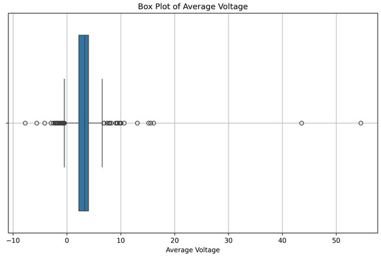
Figure 1.
Box plot of average voltage values in the dataset. The box indicates the interquartile range (IQR), and the whiskers extend to capture approximately 99% of the data range. Points outside the whiskers are identified as outliers.
Separately, to address potential outliers in the input features, a robust scaler was applied during preprocessing. This scaler adjusts feature values based on the IQR, helping to normalize the input data while reducing the influence of extreme values.
In addition to distributional imbalances in the target variable, the dataset also exhibits strong imbalance across different working ion types. Table 1 summarizes the count of samples per ion in the training, validation, and test sets. Lithium (Li)-based batteries dominate the dataset with 2440 samples, while ions such as Cs, Rb, and Y are significantly underrepresented. This class imbalance is important to consider because models trained on such skewed data may become biased toward the majority ion. To mitigate this effect, we later implement a weighted loss function during training (see Section 4.5).

Table 1.
Sample distribution by working ion across the train, validation, and test splits.
3.2. Model Architecture
Each model architecture evaluated in this study is built upon a shared backbone: a Transformer encoder applied to tabular features, followed by different regression heads tailored for voltage prediction. The base implementation uses PyTorch 2.2.1, and Figure 2 shows the structural overview of the four models.
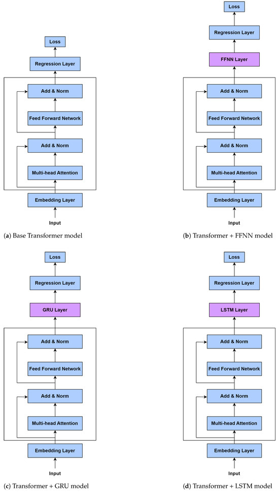
Figure 2.
Architectures of the proposed Transformer-based models.
3.2.1. Base Transformer Model
The Base Transformer architecture applies a Transformer encoder to embedded input features and directly connects it to a linear regression head. Tabular input of dimension num_features is first passed through a linear layer to project it into a high-dimensional space of dim_embedding. This embedding is reshaped to simulate a single-sequence input before being processed by a multi-layer Transformer encoder. The model uses nn.TransformerEncoderLayer with 2 attention heads and 2 encoder layers, with dropout applied at 0.2. After encoding, the outputs are aggregated using a mean operation along the sequence dimension and passed through a final linear layer to predict the target voltage:
This model offers a simple and efficient baseline for capturing feature dependencies.
3.2.2. Transformer + Feedforward Neural Network (FFNN)
This variant replaces the base model’s single regression head with a two-layer feedforward network. After the Transformer encoder, the encoded feature vector is passed through
- A hidden linear layer;
- A ReLU activation;
- Another linear layer to produce the regression output.
To preserve original feature information, a residual connection adds a weighted contribution from a parallel linear projection of the raw encoded features. The output is computed as a weighted combination of the transformed path and the residual:
where is a learnable parameter initialized to 0.5. This hybrid structure improves robustness and enables the model to better adapt to complex mappings between embeddings and target voltages.
3.2.3. Transformer + GRU
This architecture introduces temporal modeling by adding a GRU layer after the Transformer encoder. The GRU processes the output embeddings as a one-step sequence and captures latent interactions using its gated recurrence dynamics:
The GRU has one layer, 128 hidden units, and uses a dropout of 0.5. After computing the hidden state, a fully connected layer maps it to the output voltage. This setup is particularly effective for datasets with sequential or time-aware feature interactions.
3.2.4. Transformer + LSTM
This model is similar to the GRU-enhanced version but substitutes the GRU with an LSTM. The LSTM comprises a memory cell and three gates—input, forget, and output—that control information flow. It processes the Transformer outputs as a sequence and computes the final hidden state, which is then passed to a fully connected output layer. Like the GRU model, it uses 128 hidden units and a dropout of 0.5. The LSTM’s gating allows it to better retain relevant historical context, making it suitable for more complex sequence dependencies.
Each of these models shares the same embedding and Transformer encoder configuration, but the regression heads vary in complexity and inductive bias. Figure 2 provides a schematic comparison of the four models.
3.3. Evaluation Metrics
The performance of the ML model was evaluated using multiple metrics to comprehensively assess its accuracy and reliability. These metrics are commonly employed for regression tasks and provide insights into different aspects of model performance [32]. The metrics used in this study are described below.
3.3.1. Mean Absolute Error
MAE measures the average magnitude of the errors between the predicted and actual values, without considering their direction. It is calculated as:
where n is the total number of data points, is the actual value, and is the predicted value. MAE is particularly useful for understanding the model’s average deviation from the true values. Lower MAE values indicate better predictive accuracy.
3.3.2. Mean Squared Error
MSE measures the average squared difference between the predicted and actual values. It is calculated as:
This metric penalizes larger errors more heavily than smaller ones, making it sensitive to outliers. A lower MSE value indicates better model performance.
3.3.3. Score (Coefficient of Determination)
The score quantifies the proportion of variance in the target variable explained by the model. It is calculated as:
where represents the mean of the observed target values. An score of 1 indicates that the model accounts for all the variability in the target variable, reflecting perfect predictive performance. Conversely, an score of 0 suggests that the model’s predictions are no better than using as a constant baseline predictor.
3.3.4. Residual Analysis
In addition to these metrics, residual analysis was performed to evaluate the distribution of prediction errors. Residuals are defined as:
By analyzing the residuals, we assessed whether the model errors were randomly distributed and unbiased. Any systematic patterns in the residuals would indicate potential shortcomings in the model.
These evaluation metrics collectively provide a robust framework for understanding the model’s performance. While MAE and RMSE offer insights into the average prediction error, highlights the proportion of variance captured by the model. Residual analysis further ensures that the model predictions are consistent and reliable.
3.4. Composite Loss Function
The selection of an appropriate loss function is critical for training ML models, as it directly impacts their ability to learn meaningful patterns and generalize effectively to unseen data. In this study, a composite loss function was employed to combine the advantages of multiple loss components, ensuring a balanced and robust optimization process for regression tasks. Specifically, the composite loss function integrates MSE and MAE, weighted by a hyperparameter , and is defined as:
where emphasizes larger errors by squaring the differences between predicted and actual values, while measures the average absolute differences, treating all errors equally.
The use of a composite loss function is particularly well-suited for this study, as it addresses key challenges in optimizing regression models. While MSE is effective in penalizing large errors, it is highly sensitive to outliers, which can disproportionately influence the training process. This sensitivity may cause the model to overfit to extreme values, thereby reducing its overall performance on the majority of the data. On the other hand, MAE is less sensitive to outliers, as it assigns equal weight to all errors, ensuring that the model is not overly influenced by a small number of extreme deviations. By combining these two loss components, the composite loss function balances sensitivity to large errors with robustness to small variations, leading to a more stable and effective optimization process.
Another key advantage of the composite loss function is its ability to improve generalization. By leveraging the complementary strengths of MSE and MAE, the model is encouraged to minimize both average errors and extreme deviations, resulting in predictions that better capture the underlying trends in the data. This dual focus helps the model generalize more effectively to unseen samples, as confirmed by the high predictive accuracy achieved during testing.
The composite loss function also facilitates improved convergence during training. One of the challenges associated with using MSE alone is that its gradient diminishes as the errors decrease, potentially slowing down the optimization process for smaller errors. In contrast, MAE has a constant gradient magnitude, which ensures that the model continues to receive strong optimization signals even for small errors. When combined, these properties result in faster and more reliable convergence, making the training process more efficient.
An additional benefit of the composite loss function is its flexibility. The weighting factor provides control over the relative contributions of MSE and MAE to the overall loss function, allowing the approach to be tailored to the specific characteristics of the dataset. For instance, when outliers are prominent, a higher weight can be assigned to MAE to mitigate their influence. Conversely, for datasets with minimal outliers, the emphasis on MSE can be increased to ensure that larger errors are penalized more heavily.
In this study, the use of the composite loss function was particularly advantageous in handling outliers present in the dataset. The robustness introduced by MAE complemented the sensitivity of MSE, ensuring that the model learned both overall patterns and subtle nuances in the data. This was further validated through residual analysis, which showed a consistent reduction in errors across a range of predictions. By employing the composite loss function, the model achieved superior predictive performance and demonstrated its ability to handle complex regression tasks effectively.
3.5. Implementation
The models were implemented and trained using PyTorch, leveraging its flexibility for defining custom architectures and loss functions. All experiments were conducted on a Dell laptop with the following specifications: a 12th Gen Intel(R) Core(TM) i7-1255U processor running at 1.70 GHz, 16 GB of installed RAM (15.7 GB usable), and Windows 11 Home operating system (Version 23H2, OS Build 22631.4751). The training and evaluation pipelines were executed using the Python programming language with NumPy, Matplotlib, and Scikit-learn libraries for data preprocessing and visualization.
The dataset consisted of features extracted from battery materials, with the target variable being the average voltage. The data was first split into training, validation, and test sets, with 10% of the data reserved for testing and 20% of the remaining data used for validation. A RobustScaler was employed to standardize the features, ensuring resilience against outliers. The scaled data was then converted into PyTorch tensors for compatibility with the training pipeline.
Four models were developed and evaluated: Base Transformer, Transformer + FFNN, Transformer + GRU, and Transformer + LSTM. The Base Transformer model utilized a two-layer encoder with two attention heads per layer and an embedding dimension of 128. Dropout was set to 0.2 for regularization, and the regression output was computed using a linear layer after aggregating the transformer outputs with mean pooling. The Transformer + FFNN model replaced the regression layer with a two-layer feedforward neural network. This FFNN had a hidden size of 128, used ReLU activation, and incorporated a residual connection with a learnable weight parameter. For the Transformer + GRU model, a GRU-based network was added after the Transformer layers. The GRU module had a hidden size of 128, one layer, and a dropout rate of 0.5, and the final output was obtained via a linear layer. Similarly, the Transformer + LSTM architecture used an LSTM-based network with a hidden size of 128, one layer, and a dropout rate of 0.5.
All models were trained using the Adam optimizer with a learning rate of 0.00075. The loss function was a custom composite loss combining MSE and MAE, with weights assigned as 1.0 and 0.6, respectively. Each model was trained for up to 1000 epochs, except for the Transformer + FFNN model, which was trained for 2000 epochs, with early stopping used to prevent overfitting. To evaluate model performance, three metrics were used: MSE, MAE, and . These metrics provided a comprehensive assessment of the regression accuracy and the quality of predictions.
Hyperparameters were tuned manually through iterative experimentation on the validation set. We tested multiple values for key parameters, including learning rate (), batch size (), dropout rate (), and hidden size (). The final settings (learning rate = 0.00075; dropout = 0.2; hidden size = 128, batch size = 64) were selected based on the lowest validation loss and stable convergence. In addition, different loss functions were compared: MSE, MAE, and a composite (MSE + MAE). The composite formulation provided the most robust performance across ions by balancing sensitivity to large errors with resilience to outliers. All models underwent the same manual tuning process, ensuring fairness of comparison.
While the experiments were run on a system without GPU acceleration, the relatively small dataset and efficient model architectures allowed for feasible training times. For larger datasets or more complex tasks, utilizing GPU acceleration would significantly improve computational efficiency. All code and trained models are available at our public GitHub repository (https://github.com/maryvinolishaa/voltage_prediction_battery_electrode (accessed on 21 August 2025 )). Due to file size limitations, the dataset (>25 MB) is not hosted on GitHub but can be obtained from the authors upon reasonable request.
4. Results and Discussion
The Results and Discussion section presents a comprehensive analysis of the model architectures and their performance in predicting the average voltage of battery electrode materials. This section evaluates four Transformer-based models—Base Transformer, Transformer + FFNN, Transformer + GRU, and Transformer + LSTM—using standard metrics such as MSE, MAE, and . Additionally, the learning dynamics of these models are explored through loss plots, while residual plots and their statistical distributions provide further insights into error characteristics. By integrating these analyses, we aim to identify the strengths and limitations of each architecture and highlight the most effective approach for this regression task.
4.1. Performance Comparison
The performance of the four models—Base Transformer, Transformer with FFNN, Transformer with GRU, and Transformer with LSTM—was evaluated using MSE, MAE, and metrics. These metrics provide a comprehensive view of the models’ accuracy and ability to predict the average voltage of battery electrode materials.
The Base Transformer model achieved an MSE of 0.6212, an MAE of 0.4447, and an of 0.7630. While it effectively captured feature dependencies using self-attention mechanisms, its lack of a specialized regression head limited its ability to fine-tune embeddings for accurate predictions. This resulted in the lowest performance among the models.
Adding an FFNN as a regression head significantly improved performance. The Transformer + FFNN model achieved an MSE of 0.2856, an MAE of 0.2886, and an of 0.8910. This improvement highlights the effectiveness of FFNNs in mapping Transformer-extracted embeddings to accurate predictions, providing a balance between simplicity and computational efficiency.
The Transformer + GRU model incorporated sequential modeling capabilities, which enhanced its ability to capture temporal dependencies in the embeddings. With an updated MSE of 0.2943, an MAE of 0.2765, and an of 0.8877, this model demonstrated notable improvement compared to the Base Transformer model by leveraging GRU’s capability to model sequence information effectively.
Among the four models, the Transformer + LSTM demonstrated the best performance, with an MSE of 0.2588, an MAE of 0.2747, and an of 0.9012. By combining the Transformer’s powerful feature extraction with LSTM’s ability to model long-term dependencies, this architecture effectively captured complex relationships in the data, leading to superior predictive accuracy.
The results, summarized in Table 2, highlight the impact of combining Transformer-based architectures with specialized regression components. While the base Transformer serves as a strong foundation, integrating FFNN, GRU, or LSTM layers enhances the model’s predictive capabilities. The Transformer + LSTM model’s superior performance suggests that capturing long-term dependencies in the transformed feature embeddings is crucial for accurate voltage prediction.
Table 2.
Performance comparison of models.
4.2. Loss Plots
Loss plots are essential tools for evaluating the learning dynamics of ML models during training. They provide a graphical representation of the model’s loss function—both on the training and validation datasets—across epochs. The training loss reflects how well the model is fitting the training data, while the validation loss indicates how well the model generalizes to unseen data. By analyzing these curves, we can gain insights into model behavior, such as underfitting, overfitting, convergence stability, and generalization ability. In this section, we analyze the loss plots of the four proposed models to better understand their learning performance.
Figure 3 shows the training and validation loss plots for the four models: Base Transformer, Transformer + FFNN, Transformer + GRU, and Transformer + LSTM. These plots provide valuable insights into the learning behavior and generalization ability of each model across 2000 epochs. The training loss curve represents the model’s performance on the training data, while the validation loss curve reflects how well the model generalizes to unseen data.
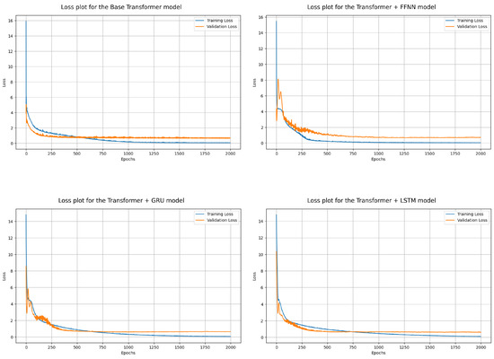
Figure 3.
Loss plots for transformer-based models: (Top-left) Base Transformer, (Top-right) Transformer + FFNN, (Bottom-left) Transformer + GRU, and (Bottom-right) Transformer + LSTM.
The Base Transformer model (top-left plot in Figure 3) exhibited steadily decreasing training loss, indicating effective optimization during training. However, the validation loss plateaued at a relatively higher value compared to other models. This discrepancy suggests that the Base Transformer struggled to generalize well to the validation data, likely due to its lack of specialized regression components. This result highlights the limitations of relying solely on the Transformer encoder for this regression task.
The Transformer + FFNN model (top-right plot) demonstrated a noticeable improvement in validation loss compared to the Base Transformer. The training and validation loss curves are more closely aligned, indicating better generalization. This improvement can be attributed to the FFNN’s role as a regression head, which enhances the model’s ability to map the learned feature embeddings to accurate predictions. The smoother loss trends also suggest that the model was less prone to overfitting than the Base Transformer.
The Transformer + GRU model (bottom-left plot) further improved the generalization capability, as evidenced by a lower validation loss compared to the previous two models. The training and validation loss curves are smoother and closer together, indicating a more stable optimization process. The GRU’s ability to capture sequential dependencies in the Transformer embeddings likely contributed to this improvement. However, the slight gap between the training and validation loss curves suggests that some degree of overfitting may still be present, particularly toward the later stages of training.
Finally, the Transformer + LSTM model (bottom-right plot) achieved the best performance among all architectures. The training and validation loss curves are both the lowest and most closely aligned, reflecting the model’s strong generalization ability and minimal overfitting. The LSTM’s advanced gating mechanisms likely played a significant role in capturing long-term dependencies in the feature embeddings, resulting in superior optimization and predictive performance. The consistent downward trend in both loss curves further indicates the robustness of this architecture.
Overall, the progressive improvement in performance across the four models underscores the importance of incorporating specialized components into the Transformer architecture for regression tasks. While the Base Transformer serves as a strong foundation for feature extraction, adding regression-specific layers such as FFNN, GRU, or LSTM enhances the model’s capacity to generalize. Among these, the Transformer + LSTM model stands out as the most effective, achieving the lowest validation loss and demonstrating the greatest alignment between training and validation loss curves.
4.3. Error Analysis Through Residuals
Residual analysis plays a critical role in evaluating the predictive performance of regression models. Residuals, defined as the difference between the true values and predicted values, reveal the degree of error associated with a model’s predictions. Ideally, residuals should follow a random distribution around zero, indicating that the model does not exhibit systematic errors. Any patterns or trends in residuals may signal underfitting, overfitting, or other modeling issues. By visualizing residuals through scatter plots and analyzing their statistical distribution, one can assess a model’s ability to generalize effectively across a dataset.
Figure 4 shows the residual plots for the four models: Base Transformer, Transformer + FFNN, Transformer + GRU, and Transformer + LSTM. These scatter plots visualize residuals as a function of predicted values, providing insight into the distribution and magnitude of errors. The Base Transformer model demonstrates significant variability in residuals, particularly at larger predicted values. The residuals exhibit higher dispersion, which may indicate that the model struggles to capture complex relationships in the data. This behavior suggests underfitting, as the model lacks sufficient capacity to generalize beyond the training dataset. Additionally, noticeable clustering patterns in the residuals suggest potential systematic errors in its predictions.
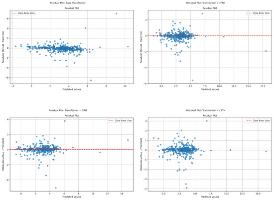
Figure 4.
Residual plots for Transformer-based models: (Top-left) Base Transformer, (Top-right) Transformer + FFNN, (Bottom-left) Transformer + GRU, and (Bottom-right) Transformer + LSTM. Each blue dot represents a residual for a single sample (difference between actual and predicted voltage).
The Transformer + FFNN model improves upon the Base Transformer by reducing the dispersion of residuals. However, residuals remain more spread out at higher predicted values, indicating the model has limited accuracy for extreme predictions. This suggests that the feedforward neural network enhances predictive performance but does not fully resolve the limitations of the Base Transformer. The Transformer + GRU model shows significant improvement in residual behavior. The residuals are more closely centered around zero, with reduced dispersion compared to the FFNN-enhanced model. The GRU’s ability to model sequential dependencies in the data likely contributes to this improvement. However, minor clustering patterns persist, suggesting slight systematic errors. The Transformer + LSTM model exhibits the most consistent and minimal residual behavior. Residuals are uniformly distributed around zero with very little spread, indicating the model’s ability to make highly accurate predictions across a wide range of values. This uniformity reflects the advanced gating mechanisms of the LSTM, which allow it to capture long-term dependencies and provide robust generalization.
Figure 5 complements the residual plots by presenting the statistical distribution of residuals for each model. These histograms illustrate the frequency of residual values, offering a quantitative perspective on error distribution. The Base Transformer exhibits a wider residual distribution, with significant variance and a lower frequency of residuals near zero. This distribution reflects greater prediction errors, particularly for edge cases in the dataset. Transformer + FFNN narrows the residual distribution, increasing the concentration of residuals around zero. This improvement suggests enhanced model accuracy, particularly for the majority of the dataset, though some edge cases still produce large errors. Transformer + GRU further refines the residual distribution. The spread decreases noticeably, and the histogram shows a sharper peak at zero. This narrowing reflects the GRU’s ability to minimize errors by effectively capturing temporal and sequential patterns in the data. Transformer + LSTM achieves the tightest residual distribution among the four models. The majority of residuals are concentrated near zero, with very few outliers, highlighting the model’s superior ability to generalize and minimize errors consistently. This tight distribution aligns with the trends observed in the residual plots and reinforces the LSTM’s position as the most accurate architecture.
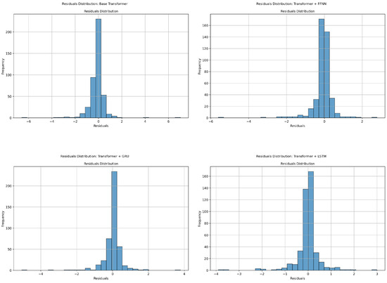
Figure 5.
Residual distribution plots for Transformer-based models: (Top-left) Base Transformer, (Top-right) Transformer + FFNN, (Bottom-left) Transformer + GRU, and (Bottom-right) Transformer + LSTM.
Together, these visualizations reveal a progressive improvement in predictive performance across the tested architectures. The Transformer + LSTM model emerges as the most effective, consistently delivering accurate predictions with minimal errors. These findings underscore the importance of residual analysis in understanding model behavior and identifying the best-performing architecture.
4.4. Uncertainty Estimation via Bootstrapping
To assess the reliability of model performance metrics, we used bootstrap resampling on the test set. Bootstrapping is a statistical method that estimates variability by repeatedly sampling, with replacement, from the original dataset. Each sample is used to compute performance metrics such as MAE, MSE, and , providing an empirical distribution for each metric.
From these distributions, we calculated the standard deviation and 95% confidence intervals. The confidence intervals were derived using the percentile method, which identifies the 2.5th and 97.5th percentiles of the bootstrapped metric values to define the lower and upper bounds of the interval. A 95% confidence interval indicates the range within which the true value of the metric is expected to lie with high probability, assuming the bootstrap samples adequately represent the population.
Table 3 presents the bootstrapped evaluation metrics for the four models, including the mean, standard deviation, and 95% confidence intervals (CI) for MAE, MSE, and . The mean represents the average model performance across 1000 bootstrap samples drawn with replacement from the test set. The ± symbol indicates the standard deviation, which reflects variability across bootstrap samples. The values in brackets denote the 95% confidence intervals, providing a statistical range within which the true metric value is likely to lie with high probability.
Table 3.
Bootstrapped mean performance metrics with standard deviation and 95% confidence intervals (CI).
Lower values of MAE and MSE indicate better predictive accuracy, while higher values (closer to 1) reflect a better fit to the true data. Among the four models, Transformer + LSTM achieved the best overall performance, showing the lowest average MSE and MAE with narrow confidence intervals. This reinforces earlier findings from the test set evaluation and suggests that the LSTM-based model generalizes robustly to new data.
4.5. Per-Ion Performance Evaluation
We analyzed how each model performs across different working ions. We computed MAE, MSE, and for each ion. Figure 6, Figure 7 and Figure 8 show these per-ion metrics. Figure 9 shows overall test set performance for each model with and without sample-wise loss weighting.
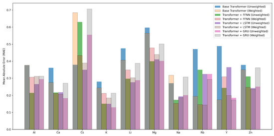
Figure 6.
Per-ion MAE across models with and without sample-wise loss weighting.
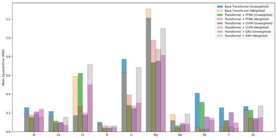
Figure 7.
Per-ion MSE across models with and without sample-wise loss weighting.
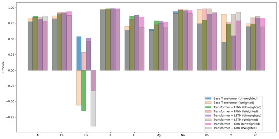
Figure 8.
Per-ion across models with and without sample-wise loss weighting.
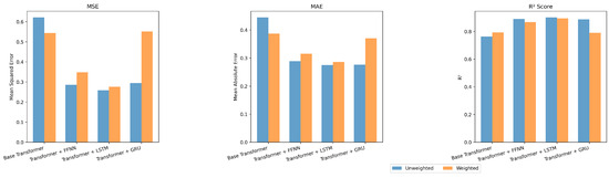
Figure 9.
Overall test performance of each model with and without sample-wise loss weighting.
In the FFNN, LSTM, and GRU models, loss weighting led to a small drop in overall performance. For example, in the FFNN model, test MAE increased from 0.2887 to 0.3154, and dropped from 0.8910 to 0.8670. This result is expected. Sample-wise loss weighting shifts attention toward ions that appear less often in the training set. This shift can reduce accuracy on more common ions. In return, it improves predictions on rare ions. In the FFNN model, the for Rb improved from 0.8036 to 0.9832. In the LSTM and GRU models, metrics for ions such as Ca, Rb, and Y also improved.
In contrast, the Base Transformer behaved differently. With sample-wise weighting, it achieved better results on both per-ion and overall metrics. Test MAE dropped from 0.4447 to 0.3873. improved from 0.7630 to 0.7925. This is surprising. Weighted loss often helps fairness but can hurt overall performance. Here, it helped both.
Why did this happen? One reason may be that the Base Transformer overfit to common ions when trained without weighting. Sample-wise weighting reduced this effect. It forced the model to learn patterns that work across many ions. This improved generalization. Another reason may be the makeup of the test set. If the test set includes many rare ions, then improving their predictions helps the overall average.
These results suggest that loss weighting helps models pay more attention to rare ions. In complex models, this comes with a trade-off. In simpler models, such as the Base Transformer, it can improve generalization and fairness at the same time.
4.6. Feature Importance via SHAP Analysis
To better understand which features most influenced each model’s predictions, we employed SHAP (SHapley Additive exPlanations). We present both global SHAP analysis, which ranks features by their overall importance across the dataset, and local SHAP analysis, which highlights case-by-case feature contributions for individual predictions.
4.6.1. Global SHAP Analysis
The global SHAP analysis visualizes the top 20 features ranked by their mean absolute SHAP values. Figure 10, Figure 11, Figure 12 and Figure 13 show the results for the Base Transformer, Transformer + FFNN, Transformer + LSTM, and Transformer + GRU models, respectively.
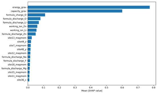
Figure 10.
Top 20 most important features for the Base Transformer model.
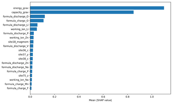
Figure 11.
Top 20 most important features for the Transformer + FFNN model.
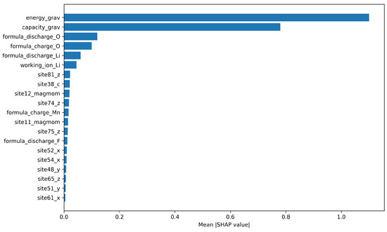
Figure 12.
Top 20 most important features for the Transformer + LSTM model.
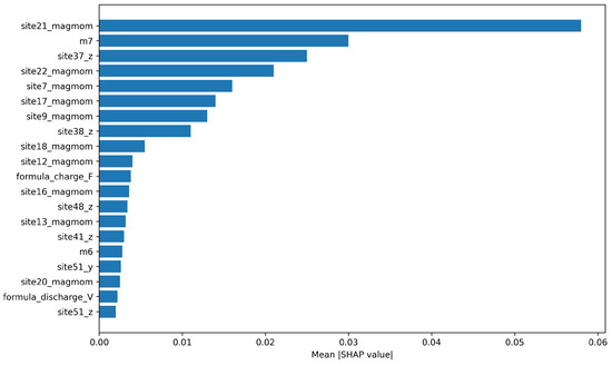
Figure 13.
Top 20 most important features for the Transformer + GRU model.
Across the Base Transformer (Figure 10), Transformer + FFNN (Figure 11), and Transformer + LSTM (Figure 12) models, energy_grav (gravimetric energy, in Wh/kg) and capacity_grav (gravimetric capacity, in mAh/g) consistently ranked as the most influential features. This suggests that these features strongly determine the electrode voltage, likely because they encapsulate key electrochemical energy and charge storage behaviors that the model learns to associate with target voltage values.
Interestingly, for the Transformer + GRU model (Figure 13), site-specific magnetic moment features such as site21_magmom and site22_magmom emerged as more important than energy_grav and capacity_grav. This divergence suggests that the GRU-based model may have relied more heavily on local structural and magnetic properties than the other architectures.
Overall, the SHAP analysis reveals both the dominant influence of energy- and capacity-related features for most models, and also highlights model-dependent differences in feature attribution.
4.6.2. Local SHAP Analysis
While global SHAP highlights the average feature importance across the dataset, local SHAP explains individual predictions. Each local SHAP plot decomposes a prediction into positive (red) and negative (blue) feature contributions relative to the model’s expected output. Red bars indicate features that increase the predicted voltage, while blue bars indicate features that decrease it. The sum of these contributions equals the model’s predicted value for that sample.
To illustrate, we focus on the best-performing Transformer + LSTM model and examine three representative cases:
- i.
- Best (minimum error): predicted = 2.4671 V; actual = 2.4671 V; |error| = 0.0000 V.
- ii.
- Median (typical error): predicted = 2.9417 V; actual = 2.8242 V; |error| = 0.1175 V.
- iii.
- Worst (maximum error): predicted = 3.2691 V; actual = 0.0455 V; |error| = 3.2235 V.
In the best case (Figure 14), energy_grav and capacity_grav dominate, and their combined contributions align the prediction almost exactly with the ground truth. In the median case (Figure 15), the same two features nearly cancel, leaving smaller formula and site-level descriptors to determine the output, which explains the moderate error. In the worst case (Figure 16), extreme values of energy_grav and capacity_grav mislead the model, while additional site descriptors amplify the deviation, resulting in a large error.
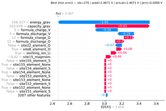
Figure 14.
Local SHAP explanation for the best (minimum error) case.
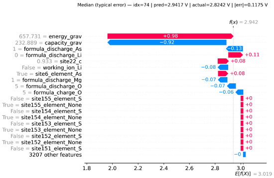
Figure 15.
Local SHAP explanation for the median (typical error) case.
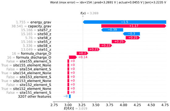
Figure 16.
Local SHAP explanation for the worst (maximum error) case.
Together, these cases demonstrate that while global SHAP identifies consistent dataset-wide drivers, local SHAP reveals how those same features can either support accurate predictions or contribute to substantial errors, depending on the sample.
The analyses presented in this section demonstrate the progressive improvement in performance achieved by incorporating specialized components into the Transformer architecture. The Base Transformer model, while effective as a foundational architecture, exhibited limitations in predictive accuracy and generalization. The addition of an FFNN enhanced the model’s ability to map embeddings to accurate predictions. Further improvements were achieved through the inclusion of sequential modeling capabilities in the Transformer + GRU and Transformer + LSTM models. Among the architectures, the Transformer + LSTM emerged as the most effective, achieving the lowest validation loss, tightest residual distribution, and highest R2 score. These findings underscore the importance of integrating advanced regression components with feature extraction techniques for improving predictive accuracy. The results highlight the potential of Transformer-based architectures in accelerating materials research and predictive modeling tasks.
5. Conclusions
This study proposed a Transformer-based deep learning model to predict the average voltage of battery electrode materials. By leveraging the Transformer architecture’s ability to capture complex relationships and long-range dependencies, the model demonstrated superior performance compared to existing methods. It achieved lower MAE and MSE, as well as higher R2 values, outperforming all prior studies in the field. These results validate the effectiveness of the Transformer model for regression tasks in materials science.
The model’s success highlights the potential of ML to accelerate the discovery of promising electrode materials for energy storage applications. However, our evaluation is restricted to MP-calculated voltages and does not include experimental validation or cross-database testing. As such, the reported performance reflects in-distribution error on MP and may not transfer directly to experimental measurements or to datasets curated under different protocols.
Future work should therefore incorporate external test sets, experimental benchmarks, and additional material datasets, while also integrating domain knowledge to further enhance prediction accuracy. This advancement supports the transition toward sustainable and efficient battery technologies.
Author Contributions
Methodology, M.V.A.D. and E.O.E.; Formal analysis, M.V.A.D. and A.I.A.; Investigation, M.V.A.D. and I.B.; Data curation, M.V.A.D.; Writing—original draft, M.V.A.D.; Writing—review & editing, I.B., E.O.E. and A.I.A.; Supervision, I.B. All authors have read and agreed to the published version of the manuscript.
Funding
This research received no external funding.
Data Availability Statement
The original contributions presented in this study are included in the article. Further inquiries can be directed to the corresponding author.
Conflicts of Interest
The authors declare no conflicts of interest.
References
- Fichtner, M.; Edström, K.; Ayerbe, E.; Berecibar, M.; Bhowmik, A.; Castelli, I.E.; Clark, S.; Dominko, R.; Erakca, M.; Franco, A.A.; et al. Rechargeable Batteries of the Future—The State of the Art from a BATTERY 2030+ Perspective. Adv. Energy Mater. 2022, 12, 2102904. [Google Scholar] [CrossRef]
- Fekete, B.; Bacskó, M.; Zhang, J.; Chen, M. Storage requirements to mitigate intermittent renewable energy sources: Analysis for the US Northeast. Front. Environ. Sci. 2023, 11, 1076830. [Google Scholar] [CrossRef]
- Armand, M.; Tarascon, J.M. Building Better Batteries. Nature 2008, 451, 652–657. [Google Scholar] [CrossRef] [PubMed]
- Desaulty, A.M.; Climent, D.M.; Lefebvre, G.; Cristiano-Tassi, A.; Peralta, D.; Perret, S.; Urban, A.; Guerrot, C. Tracing the origin of lithium in Li-ion batteries using lithium isotopes. Nat. Commun. 2022, 13, 4172. [Google Scholar] [CrossRef]
- Cutting cobalt. Nat. Energy 2020, 5, 825. [CrossRef]
- Park, G.T.; Namkoong, B.; Kim, S.B.; Liu, J.; Yoon, C.; Sun, Y.K. Introducing high-valence elements into cobalt-free layered cathodes for practical lithium-ion batteries. Nat. Energy 2022, 7, 946–954. [Google Scholar] [CrossRef]
- Naseer, M.N.; Serrano-Sevillano, J.; Fehse, M.; Bobrikov, I.; Saurel, D. Silicon anodes in lithium-ion batteries: A deep dive into research trends and global collaborations. J. Energy Storage 2025, 111, 115334. [Google Scholar] [CrossRef]
- Urban, A.; Seo, D.H.; Ceder, G. Computational understanding of Li-ion batteries. Npj Comput. Mater. 2016, 2, 16002. [Google Scholar] [CrossRef]
- Jain, A.; Shin, Y.; Persson, K. Computational predictions of energy materials using density functional theory. Nat. Rev. Mater. 2016, 1, 15004. [Google Scholar] [CrossRef]
- Ling, C. A review of the recent progress in battery informatics. Npj Comput. Mater. 2022, 8, 33. [Google Scholar] [CrossRef]
- Xia, B.; Qin, Z.; Fu, H. Rapid estimation of battery state of health using partial electrochemical impedance spectra and interpretable machine learning. J. Power Sources 2024, 603, 234413. [Google Scholar] [CrossRef]
- Joshi, R.P.; Eickholt, J.; Li, L.; Fornari, M.; Barone, V.; Peralta, J.E. Machine Learning the Voltage of Electrode Materials in Metal-ion Batteries. arXiv 2019, arXiv:1903.06813. [Google Scholar] [CrossRef] [PubMed]
- Louis, S.Y.; Siriwardane, E.M.D.; Joshi, R.P.; Omee, S.S.; Kumar, N.; Hu, J. Accurate Prediction of Voltage of Battery Electrode Materials Using Attention-Based Graph Neural Networks. ACS Appl. Mater. Interfaces 2022, 14, 26587–26594. [Google Scholar] [CrossRef]
- Zhang, X.; Zhou, J.; Lu, J.; Shen, L. Interpretable learning of voltage for electrode design of multivalent metal-ion batteries. Npj Comput. Mater. 2022, 8, 175. [Google Scholar] [CrossRef]
- Yao, Z.; Lum, Y.; Johnston, A.; Mejia-Mendoza, L.M.; Zhou, X.; Wen, Y.; Aspuru-Guzik, A.; Sargent, E.H.; Seh, Z.W. Machine learning for a sustainable energy future. Nat. Rev. Mater. 2023, 8, 202–215. [Google Scholar] [CrossRef]
- Correa-Baena, J.P.; Hippalgaonkar, K.; van Duren, J.; Jaffer, S.; Chandrasekhar, V.R.; Stevanovic, V.; Wadia, C.; Guha, S.; Buonassisi, T. Accelerating Materials Development via Automation, Machine Learning, and High-Performance Computing. Joule 2018, 2, 1410–1420. [Google Scholar] [CrossRef]
- Babar, M.; Parks, H.L.; Houchins, G.; Viswanathan, V. An accurate machine learning calculator for the lithium-graphite system. J. Phys. Energy 2020, 3, 014005. [Google Scholar] [CrossRef]
- Allam, O.; Cho, B.W.; Kim, K.C.; Jang, S.S. Application of DFT-based machine learning for developing molecular electrode materials in Li-ion batteries. RSC Adv. 2018, 8, 39414–39420. [Google Scholar] [CrossRef]
- Hossain, S.M.; Koshi, N.A.; Lee, S.C.; Das, G.P.; Bhattacharjee, S. Deep Neural Network-Based Voltage Prediction for Alkali-Metal-Ion Battery Materials. arXiv 2025, arXiv:2503.13067. [Google Scholar]
- Deng, W.; Le, H.; Nguyen, K.T.; Gogu, C.; Medjaher, K.; Morio, J.; Wu, D. A generic physics-informed machine learning framework for battery remaining useful life prediction using small early-stage lifecycle data. Appl. Energy 2025, 384, 125314. [Google Scholar] [CrossRef]
- Navidi, S.; Thelen, A.; Li, T.; Hu, C. Physics-informed machine learning for battery degradation diagnostics: A comparison of state-of-the-art methods. Energy Storage Mater. 2024, 68, 103343. [Google Scholar] [CrossRef]
- Rieger, L.H.; Flores, E.; Nielsen, K.F.; Norby, P.; Ayerbe, E.; Winther, O.; Vegge, T.; Bhowmik, A. Uncertainty-aware and explainable machine learning for early prediction of battery degradation trajectory. Digit. Discov. 2023, 2, 112–122. [Google Scholar] [CrossRef]
- Tao, S.; Sun, C.; Fu, S.; Wang, Y.; Ma, R.; Han, Z.; Sun, Y.; Li, Y.; Wei, G.; Zhang, X.; et al. Battery Cross-Operation-Condition Lifetime Prediction via Interpretable Feature Engineering Assisted Adaptive Machine Learning. ACS Energy Lett. 2023, 8, 3269–3279. [Google Scholar] [CrossRef]
- Jiang, B.; Gent, W.E.; Mohr, F.; Das, S.; Berliner, M.D.; Forsuelo, M.; Zhao, H.; Attia, P.M.; Grover, A.; Herring, P.K.; et al. Bayesian learning for rapid prediction of lithium-ion battery-cycling protocols. Joule 2021, 5, 3187–3203. [Google Scholar] [CrossRef]
- Liu, K.; Niri, M.F.; Apachitei, G.; Lain, M.; Greenwood, D.; Marco, J. Interpretable machine learning for battery capacities prediction and coating parameters analysis. Control Eng. Pract. 2022, 124, 105202. [Google Scholar] [CrossRef]
- Zhang, H.; Li, Y.; Zheng, S.; Lu, Z.; Gui, X.; Xu, W.; Bian, J. Battery lifetime prediction across diverse ageing conditions with inter-cell deep learning. Nat. Mach. Intell. 2025, 7, 270–277. [Google Scholar] [CrossRef]
- Tang, A.; Xu, Y.; Tian, J.; Shu, X.; Yu, Q. Physics-informed battery degradation prediction: Forecasting charging curves using one-cycle data. J. Energy Chem. 2025, 101, 825–836. [Google Scholar] [CrossRef]
- Guirguis, J.; Ahmed, R. Transformer-Based Deep Learning Models for State of Charge and State of Health Estimation of Li-Ion Batteries: A Survey Study. Energies 2024, 17, 3502. [Google Scholar] [CrossRef]
- Huang, X.; Tao, S.; Liang, C.; Ma, R.; Wang, X.; Xia, B.; Zhang, X. Robust and generalizable lithium-ion battery health estimation using multi-scale field data decomposition and fusion. J. Power Sources 2025, 642, 236939. [Google Scholar] [CrossRef]
- Jia, C.; Tian, Y.; Shi, Y.; Jia, J.; Wen, J.; Zeng, J. State of health prediction of lithium-ion batteries based on bidirectional gated recurrent unit and transformer. Energy 2023, 285, 129401. [Google Scholar] [CrossRef]
- Shi, Y.; Wang, L.; Liao, N.; Xu, Z. Lithium-Ion Battery Degradation Based on the CNN-Transformer Model. Energies 2025, 18, 248. [Google Scholar] [CrossRef]
- Analytics Vidhya. Know The Best Evaluation Metrics for Your Regression Model. 2021. Available online: https://www.analyticsvidhya.com/blog/2021/05/know-the-best-evaluation-metrics-for-your-regression-model/ (accessed on 21 August 2025).
Disclaimer/Publisher’s Note: The statements, opinions and data contained in all publications are solely those of the individual author(s) and contributor(s) and not of MDPI and/or the editor(s). MDPI and/or the editor(s) disclaim responsibility for any injury to people or property resulting from any ideas, methods, instructions or products referred to in the content. |
© 2025 by the authors. Licensee MDPI, Basel, Switzerland. This article is an open access article distributed under the terms and conditions of the Creative Commons Attribution (CC BY) license (https://creativecommons.org/licenses/by/4.0/).