A Pressure Wave Recognition and Prediction Method for Intelligent Sliding Sleeve Downlink Communication Systems Based on LSTM

Abstract

To address the challenges of signal recognition and prediction in intelligent sliding sleeve downlink communication systems, this paper proposes a dual-model framework based on Long Short-Term Memory (LSTM) networks. The system comprises a classifier for identifying pressure wave edge types and a generator for predicting pressure waveforms. High-quality training data are generated by simulating pressure wave propagation caused by throttle valve modulations. A sliding window strategy and Z-score normalization are applied to enhance temporal modeling. The classifier achieves a high accuracy in identifying rising and falling edges under noise-free conditions. The generator, trained on down-sampled waveform segments, accurately reconstructs pressure dynamics using a dual-input strategy based on historical segments and hypothetical labels. A residual-based decision mechanism is employed to complete the full sequence label prediction. To evaluate robustness, noise intensities of 30 dB and 40 dB are introduced. The proposed system maintains high performance under both conditions, achieving label prediction accuracies of 100%. Error metrics such as MAE and RMSE remain within acceptable bounds, even in noisy environments. The results demonstrate that the proposed LSTM-based method has been validated on simulated data, showing its potential to approximate performance in real-world conditions. It provides a promising solution for cable-free measurement-while-drilling (MWD) and remote control of intelligent sliding sleeves in complex downhole environments.

1. Introduction

With the continuous advancement of unconventional oil and gas exploration and development, intelligent completion technology has gradually become a key development direction in oilfield construction [1]. Horizontal well drilling and completion technology is particularly effective for developing unconventional reservoirs such as tight oil and gas formations [2]. As a core tool in intelligent completion systems, intelligent sliding sleeves enable the remote layered control of multilateral and multi-zone wellbores, thereby significantly improving the level of intelligent production management [3].

To optimize traditional fracturing techniques, several ground-controlled downhole sleeve activation methods have been developed, including RFID-tagged balls [4,5], hydraulic control systems, and electromagnetic communication technologies [6]. However, these technologies face various limitations under conditions of deep wells, long horizontal sections and high-pressure wellbores. For example, RFID-based sleeves must be pre-opened at the sleeve tail, leading to high risks of malfunction; electromagnetic communication suffers from severe signal attenuation in formations with high resistivity or in ultra-deep wells, making signal identification challenging. Therefore, there is an urgent need for a communication method that can reliably transmit signals and accurately control sleeve activation in high-pressure, high-depth, and high-noise environments [7].

In downhole data transmission, there are two main types of signal transmission methods: wired and wireless. Wired transmission primarily includes intelligent drill pipe and fiber-optic communication, while wireless transmission mainly consists of electromagnetic waves, acoustic waves, and mud pulse transmission [8]. Recently, pressure wave communication technology based on wellbore fluid media has emerged as a promising downlink communication solution due to its cable-free design, deployment flexibility, low cost, and strong anti-interference capabilities [9,10,11]. This technique transmits encoded signals by injecting specially modulated pressure pulses into the wellbore. However, the complex downhole environment causes nonlinear signal distortion and blurred edge features and further introduces discontinuities in the sequence owing to the presence of stitching segments, making signal decoding challenging [12,13,14,15,16]. Mud Pulse Telemetry (MPT) is the most widely used measurement-while-drilling (MWD) technology and can be mainly categorized into positive pulse, negative pulse, and continuous wave systems. Among them, continuous wave telemetry is a relatively recent development. Compared to the other two methods, it offers advantages such as higher transmission rates, better reliability, and greater cost-effectiveness [17].

Deep learning has recently demonstrated powerful capabilities in sequence modeling. In traditional machine learning algorithms, such as Support Vector Machines (SVMs) [18], Decision Trees [19], Random Forests [20], and CNN, the slow training speed and sensitivity to noise in time-series data cause these algorithms to behave poorly regarding prediction. Recurrent Neural Networks (RNNs) are capable of identifying semantic patterns from input sequences [21,22]. Classical RNNs are based on multilayer perceptron architectures and are characterized by additional feedback connections. Currently, neural networks based on Long Short-Term Memory (LSTM) have attracted significant attention. Compared to traditional machine learning algorithms, LSTM networks have become widely used in fields such as speech recognition and biomedical signal processing because of their high ability to capture long-term dependencies [23,24,25]. However, the application of LSTM in downhole pressure wave communication recognition and prediction remains limited. Considering the periodic edge structures and nonlinear perturbations in pressure wave sequences [26], LSTM has theoretical advantages, yet its training and prediction strategies need to be adapted to actual downhole conditions.

To address this, this paper proposes a pressure wave recognition and prediction method for intelligent sliding sleeve downlink communication systems based on LSTM. A dual-model structure is designed, consisting of an edge-type classifier and a waveform generator. The classifier identifies the edge type of the first segment in each physical wave group, while the generator predicts future waveforms under different label hypotheses and determines the most likely label based on residual errors. To improve temporal robustness, a stitching-segment skipping mechanism and a sliding-window recursive strategy are introduced. The experimental results show that the proposed method achieves over 80% classification accuracy on pressure wave data.

2. Method

2.1. Intelligent Sliding Sleeve Model

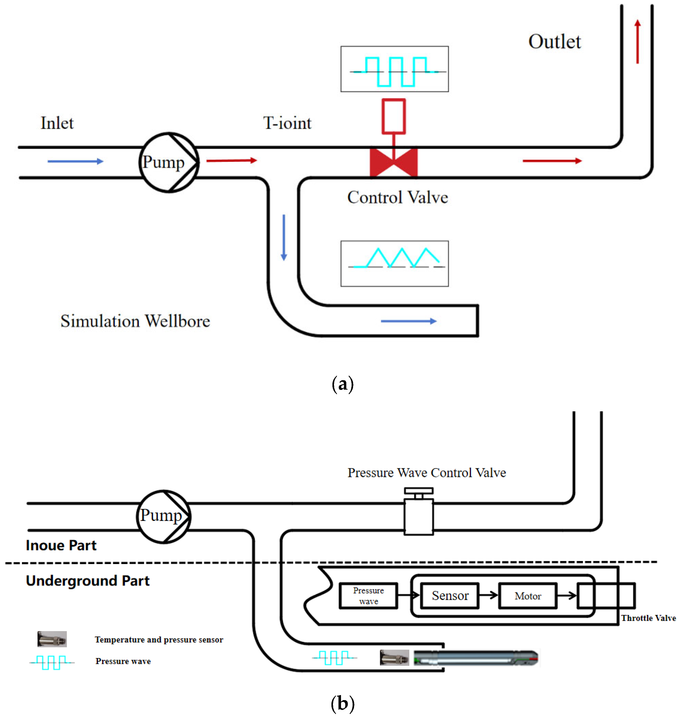
The intelligent sliding sleeve communication system using a pressure wave is shown in Figure 1. It mainly consists of a pressure pump, a T-joint, a shut-off solenoid valve, the wellbore, and the bottomhole. The pump provides a high-pressure mud flow, which serves as the signal carrier. The T-joint divides the high-pressure flow into a main flow path and a signal modulation branch. The solenoid valve controls the flow rate to generate continuous wave signals, and the valve is controlled by a personal computer, where the opening and closing operations create pressure fluctuations. As demonstrated by Stosiak et al. [27], when a proportional directional valve is subjected to external mechanical vibrations, pressure pulsations arise at frequencies corresponding to the excitation frequency. This suggests that the frequency of pressure pulsations generated during valve operation is not only determined by the control signal frequency but is also strongly influenced by the mechanical dynamics of the valve itself. The wellbore serves as the transmission path through which the signal travels down the drill string or returns from the bottom. The bottomhole is where the signal modulation device or measuring instrument is located, acting as the terminal point of signal propagation, as well as the location for pressure wave signal sampling and decoding [28].

Neglecting the influence of the pump piston stroke, the pump displacement can be described as follows:

$$Q_{pump}=Q_0$$

(1)

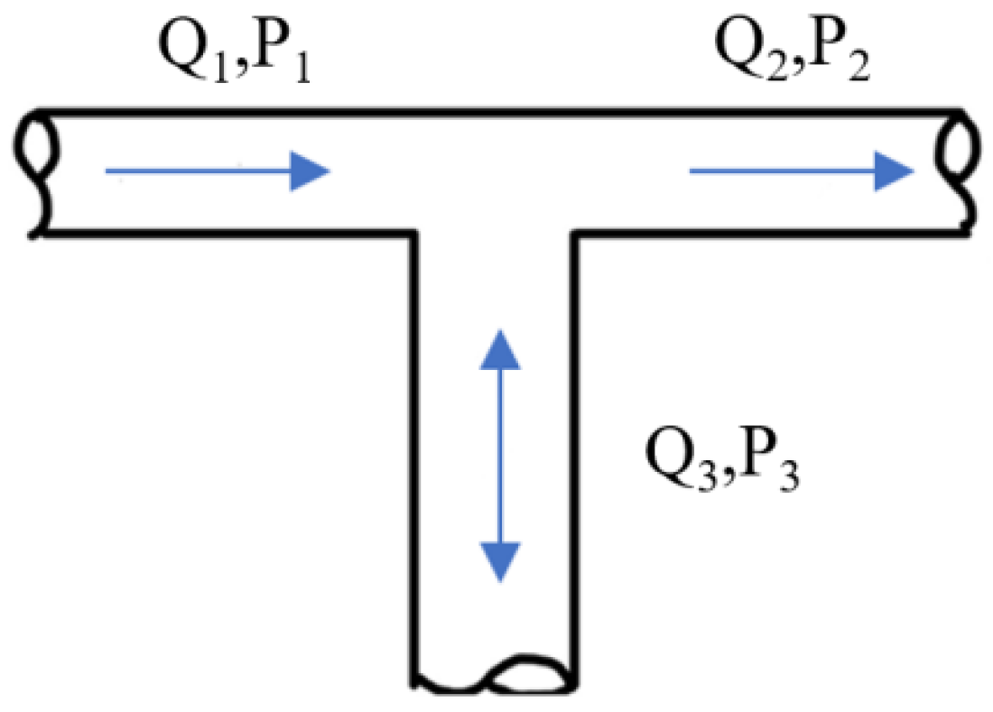
The T-joint is installed between the pump, the throttle valve, and the bottomhole and is connected through pipelines. As the name implies, the T-joint has three flow paths, as illustrated in the Figure 2 below [29]:

Under ideal conditions, the continuity equations for the T-joint are as follows:

$$Q_1=Q_2+Q_3$$

(2)

$$P_1=P_2=P_3$$

(3)

The throttle valve serves as the boundary condition for the downlink system. As shown in Figure 3, the variation in the valve opening can be described by the following rules [29]:

$$\tau ={\left(1-{{\displaystyle \frac{t}{t}}}_c\right)}^m$$

(4)

where τ is the opening of the throttle valve; t is the relative time of valve closing or opening; t_c is the time to close the throttle valve; and m is the coefficient factor of the control valve.

The pressure loss at the throttle valve is related to the degree of valve opening and closing and can be expressed by the following relationship:

$$Q_{in}=Q_{out}=Q_v={\displaystyle \frac{Q_0\tau }{\sqrt{P_0}}}\sqrt{P_{in}-P_{out}}$$

(5)

where P₀ is a known pressure loss.

2.2. Model Validation

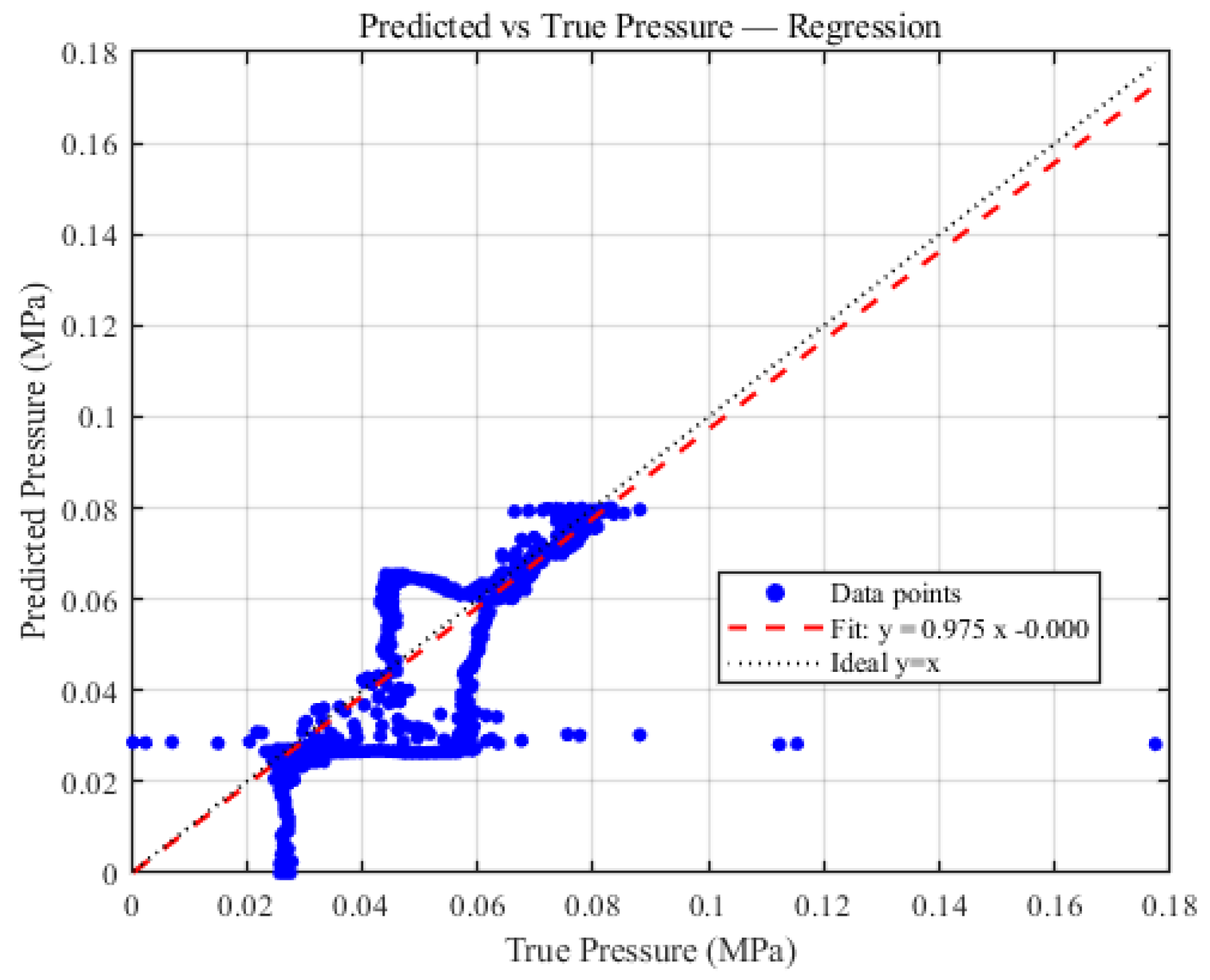
Figure 4 shows the comparison between the measured pressure at the pump and the model-predicted pressure when the electromagnetic valve is closed for 10 s. It is clearly observed from the regression plot that the model fitting results closely match the experimental test data. The fitted curve follows the equation y = 0.975x, which is very close to the ideal line.

As shown in the regression plot, a deviation is observed between the experimental data and the predicted data when the pressure is below 0.06 MPa. This is because the rapid opening of the electromagnetic valve from the closed state causes a sudden surge in flow rate, which triggers instantaneous pressure fluctuations and generates strong pressure pulses or oscillations in the system. Additionally, the pipeline materials used in the experimental setup are not uniform, leading to reflection and scattering of pressure waves during propagation. When coupled with the abrupt valve action, these effects are further amplified, resulting in larger pressure deviations.

In contrast, when the pressure exceeds 0.06 MPa, the predicted data fit the experimental data well. This indicates that once the electromagnetic valve reaches a stable open state, the prediction model achieves good agreement with the experimental system and can accurately capture the pressure behavior.

2.3. LSTM Model

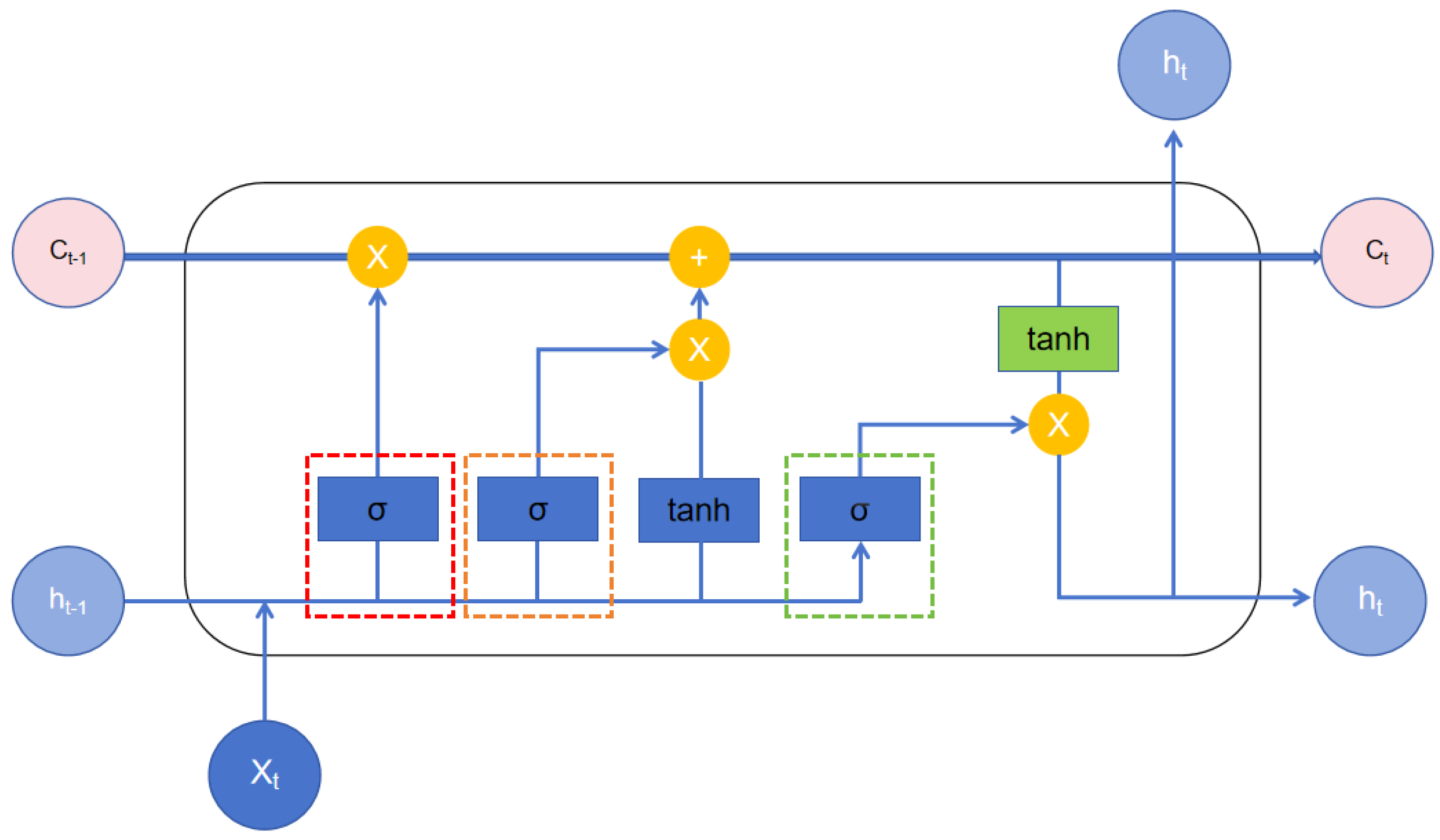
Long Short-Term Memory (LSTM) is a special type of Recurrent Neural Network (RNN) architecture designed specifically to cope with long-term dependency issues in sequential data processing and prediction. Traditional RNNs tend to be involved in diminishing influence of earlier inputs when handling long sequences. The structure of the LSTM model is shown in Figure 5. It includes the forget gate, input gate, and output gate. Here, σ represents the sigmoid function, which determines the importance of the current input information, while the tanh function generates new candidate values used to update the cell state. LSTM overcomes this by introducing a gating mechanism—including the input gate, forget gate, and output gate—as illustrated in the basic structure diagram. This mechanism enables the network to retain important historical information while suppressing irrelevant signals, thereby enhancing performance in tasks such as speech recognition, natural language processing, and industrial time-series signal modeling. In this study, LSTM is applied to model downhole pressure wave time-series data for effective signal recognition and prediction.

In cable-free measurement-while-drilling (MWD) systems, downhole information is typically transmitted and encoded in the form of pressure waves. Accurate identification of key edge features in mud pressure wave signals (such as rising and falling edges) is crucial for high-precision signal decoding. However, under actual working conditions, pressure wave signals exhibit significant nonlinearity and nonstationary, which are subject to strong background noise, making traditional feature engineering or static statistical classification methods inadequate for capturing dynamic signal variations.

While advanced architectures such as transformers provide powerful long-range dependency modeling and faster parallel computation, they typically demand large datasets and high computational resources. In contrast, LSTMs remain highly effective in scenarios with moderate data size and strong sequential structure, such as pressure wave decoding, making them a practical choice for many industrial signal processing tasks.

In the present study, an LSTM-based approach is introduced for modeling and recognizing pressure wave signals. Compared with traditional methods, LSTM can effectively leverage historical information of pressure waves and automatically learn underlying pattern differences in signal transitions, thereby enabling the precise identification of rising and falling edges.

In this research, a large-scale dataset of simulated pressure wave samples is used to construct the training set. Segmented sparse sampling and normalization preprocessing are applied before feeding the data into the LSTM network for training and prediction.

2.4. Classifier and Generator

To enable decoding and predictive simulation of downhole pressure wave signals, this study designs and constructs an edge-type classifier and a waveform generator based on LSTM models. The classifier takes normalized pressure segments as input and extracts temporal features from the sequence to determine the edge type of the current segment (rising edge, falling edge, or splicing segment), thereby achieving accurate recognition of communication signals. Compared to traditional feature engineering methods, the LSTM-based classifier demonstrates significant advantages in modeling the nonlinear propagation characteristics of pressure waves in the wellbore. These pressure signals are influenced by complex fluid–structure interactions, valve-induced disturbances, and multiple reflections within the confined space, all of which introduce long-term temporal dependencies. The LSTM architecture is particularly well-suited for capturing such dynamics, enabling the more accurate identification of rising and falling edges in downhole communication.

Meanwhile, to simulate the actual pressure response within the downhole channel, a waveform generator based on LSTM is also developed. This generator takes historical segments and preset edge labels as dual inputs to learn the evolution patterns of different signal types in the wellbore and outputs the predicted future pressure waveform. The classifier utilizes an LSTM model to perform normalized feature extraction on the input pressure wave signals. By leveraging a large amount of feature and label data for deep learning, it can effectively recognize pressure waves and output the corresponding label values. The generator also adopts an LSTM model for training; however, unlike the classifier, it uses a dual-input structure, simultaneously taking in the normalized historical pressure segment and the label of the predicted segment. Through deep learning with a large number of training samples, the generator is ultimately able to output the predicted waveform segment. The strategy of training the classifier and generator separately ensures that both modules maintain high signal recognition accuracy during operation. When used sequentially in a combined manner, they can effectively identify signals within continuous pressure waves.

2.5. Model Prediction

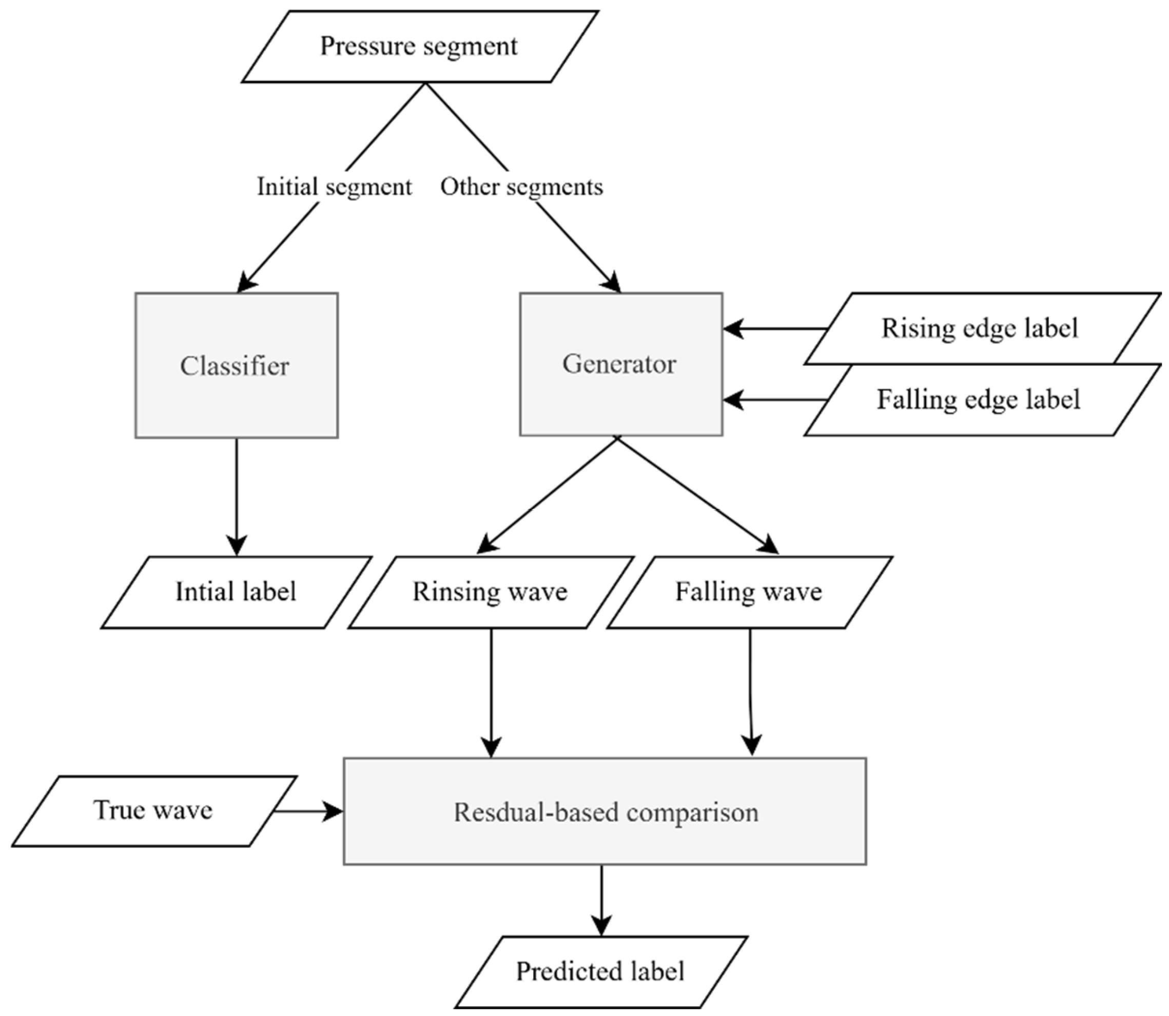
Before model prediction, the classifier and generator are trained separately. The classifier is responsible for identifying the rising or falling edge labels of pressure wave segments, while the generator produces the corresponding pressure waveform based on the input label. A complete pressure waveform consists of eight physical subsegments, each corresponding to a label. During prediction, the first segment cannot be inferred from historical data and must be classified using the trained classifier. For the remaining segments, labels are obtained through the generator: the historical pressure waveform and a hypothesized label (either rising edge “0” or falling edge “1”) are jointly fed into the generator to produce two predicted waveforms. These predicted waveforms are then compared with the actual future segment using residual error. The label of the predicted segment with the smaller residual is assigned to the true segment. The model prediction process is illustrated in Figure 6. This approach enables the complete labeling of the pressure waveform and achieves accurate decoding of the time-series signal.

2.6. Performance Evaluation

To evaluate the accuracy and effectiveness of the trained machine learning model, four performance metrics are employed: Mean Squared Error (MSE), Coefficient of Determination (R²), Root Mean Squared Error (RMSE), and Mean Absolute Error (MAE) [30,31,32,33].

$$\mathrm{M}\mathrm{S}\mathrm{E}={\displaystyle \frac{1}{N}}{\sum }_{i=1}^N{(p_i-f_i)}^2$$

(6)

$${\mathrm{R}}^2=1-{\displaystyle \frac{{\sum }_{n=1}^N{(p_i-f_i)}^2}{{\sum }_{n=1}^N{(f_i-O_{avg})}^2}}$$

(7)

$$\mathrm{R}\mathrm{M}\mathrm{S}\mathrm{E}=\sqrt{{\displaystyle \frac{1}{N}}{\sum }_{i=1}^N{(p_i-f_i)}^2}$$

(8)

$$\mathrm{M}\mathrm{A}\mathrm{E}={\displaystyle \frac{1}{N}}{\sum }_{n=1}^N|p_i-f_i|$$

(9)

where N is the number of data points; p_i is the predicted value by the model; f_i is the actual value; and O_avg is the average of the actual values.

MSE reflects the “energy” of the prediction error by averaging the squared differences between predicted and true values. RMSE, as its square root, provides a more intuitive measure of the typical prediction deviation. The coefficient of determination, R², quantifies how well the model explains the variability in the actual data, where R² = 1 indicates a perfect fit. MAE computes the average of the absolute errors across all data points, offering a straightforward interpretation of the model’s average prediction error.

In the context of downhole pressure wave communication for intelligent sleeve control, practical applications typically require the RMSE and MAE to be below 0.1 MPa to ensure reliable signal decoding and actuation. An R² value above 0.80 is generally considered acceptable for capturing the main signal trends, while values exceeding 0.90 indicate high-fidelity prediction performance.

3. Data Generation and Preprocessing

3.1. Pressure Wave Data Generation

Based on the simulation parameters listed in

Table 1. Parameters of simulation.

Number	Name	Symbol	Value	Unit
1	Density of fluid	ρ	1000	kg/m3
2	Velocity of the pressure wave	c	1250	m/s
3	Flow of pump	Q0	0.001	m3/s
4	Parameter of pump	a1	0.01	/
5	Parameter of pump	a2	0.1	/
7	Distance Between the pump and the T-joint	L1	10	m
8	Distance Between the T-joint and the throttle valve	L2	10	m
9	Diameter of the surface pipe	D	41	mm

, a mathematical model was developed to comprehensively simulate the pressure wave propagation process within the pressure wave communication system. The simplified system workflow is illustrated in Figure 7. First, a randomly generated 8-bit code consisting of 0s and 1s is input. Each “0” or “1” represents a change in the throttle valve opening: “0” corresponds to a closed state, while “1” corresponds to an open state. The default state of the throttle valve is half-open. By controlling the variation in the throttle valve’s opening, the pressure within the wellbore can be modulated. An increase in valve opening leads to a decrease in the amplitude of the pressure wave, appearing as a falling edge within the time window of a single code bit. Conversely, a decrease in valve opening leads to an increase in the pressure wave amplitude, manifesting as a rising edge within the same time frame.

In this study, the on–off state of the control valve is governed by binary control signals, which are transmitted using Return-to-Zero (RZ) encoding [34,35]. The valve’s on–off state is represented by binary digital signals (0 and 1), where 0 indicates the valve is closed, and 1 indicates the valve is open. To ensure good timing synchronization during the transmission of the control signal, RZ encoding has been employed.

RZ encoding causes the signal level to change during each bit transmission, preventing the issue of prolonged periods with the same signal level, which is common in traditional encoding methods, and thus solving the timing synchronization problem. Specifically, in RZ encoding, 0 is represented by a low voltage level, while 1 is represented by a high voltage level. At the end of each bit period, the signal returns to the zero level. This encoding method has strong anti-interference capability, ensuring that the control signal is reliably and accurately transmitted to the receiver, even in noisy environments.

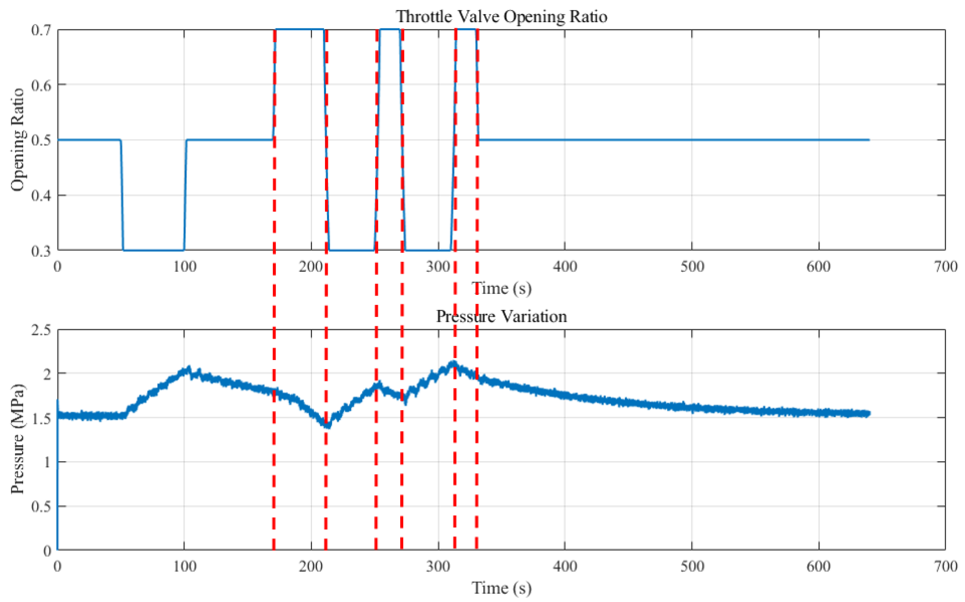
In this section, numerical simulations of the communication process are conducted. An 8-bit signal command, with each bit randomly set to either “0” or “1”, is used to control the throttle valve. The command is set such that when the signal is “1”, the valve is in the fully open state with an opening degree of 0.7. When the signal is “0”, the valve is in the fully closed state with an opening degree of 0.3. If no signal is input, the valve is in a semi-open state with an opening degree of 0.5. Figure 8 shows the valve opening variation and the pressure variation when the command signal is “11001001”, with a code length of 20 s and a noise strength of −20 dB. It is clear that the valve opening changes accurately with the input of the control signal.

Since the throttle valve is located at the bypass outlet of the T-joint structure, the drilling fluid primarily flows into the wellbore along the main channel. The throttle valve controls a portion of the fluid that discharges through the bypass outlet. When the opening of the valve increases, more fluid flows into the bypass, enhancing the bypass pressure relief capability and thereby reducing the flow rate into the wellbore. According to the relationship between pressure and flow rate, the pressure in the wellbore decreases. Conversely, when the opening of the valve decreases, the pressure in the wellbore increases.

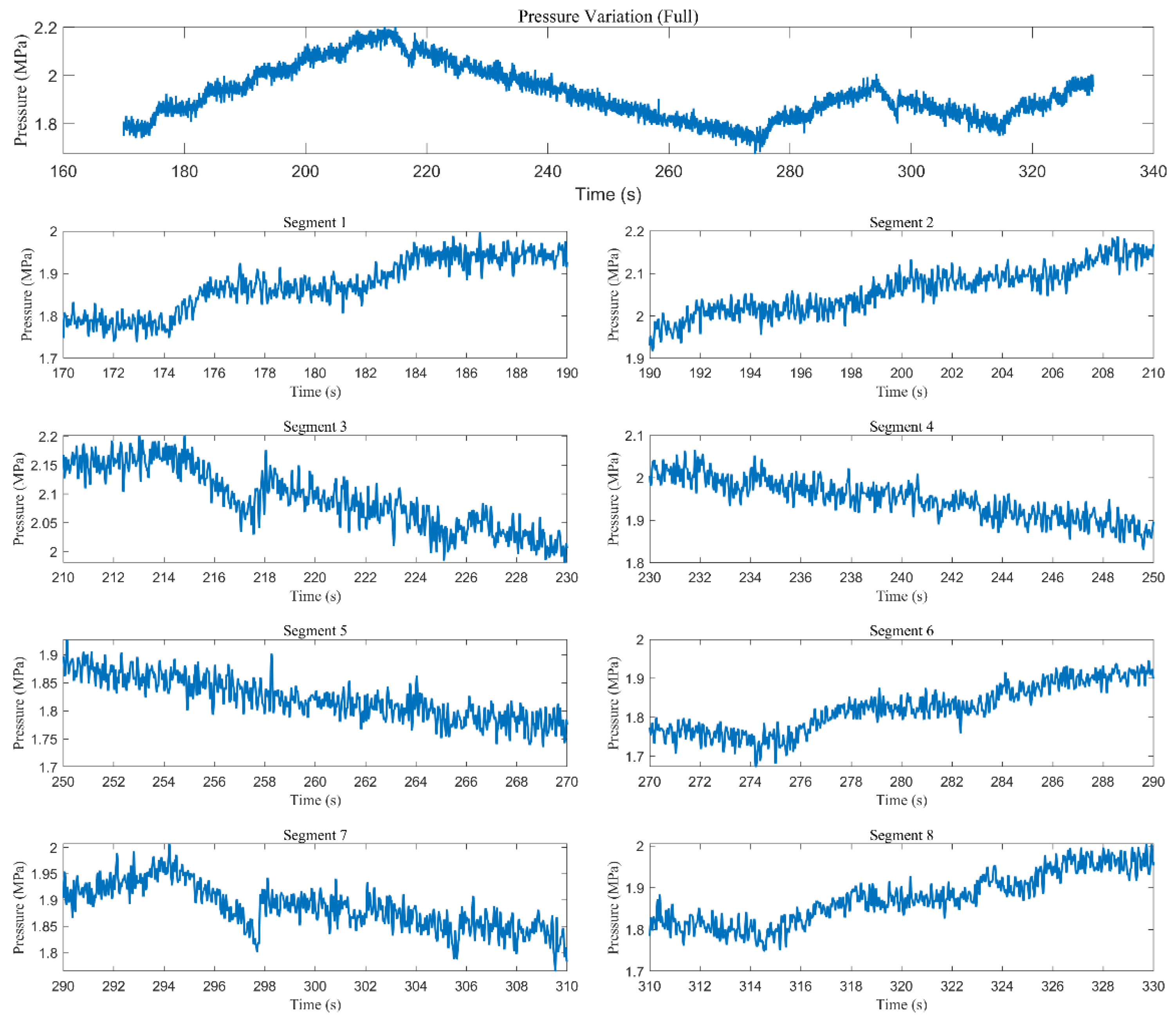
The label data sequence corresponding to the pressure wave signal is generated randomly. To simulate the actual downhole working environment, noise is added to the original pressure wave data. As shown in Figure 9, when the data sequence is “00111001” and the label duration is 20 s, the resulting pressure wave simulation is obtained.

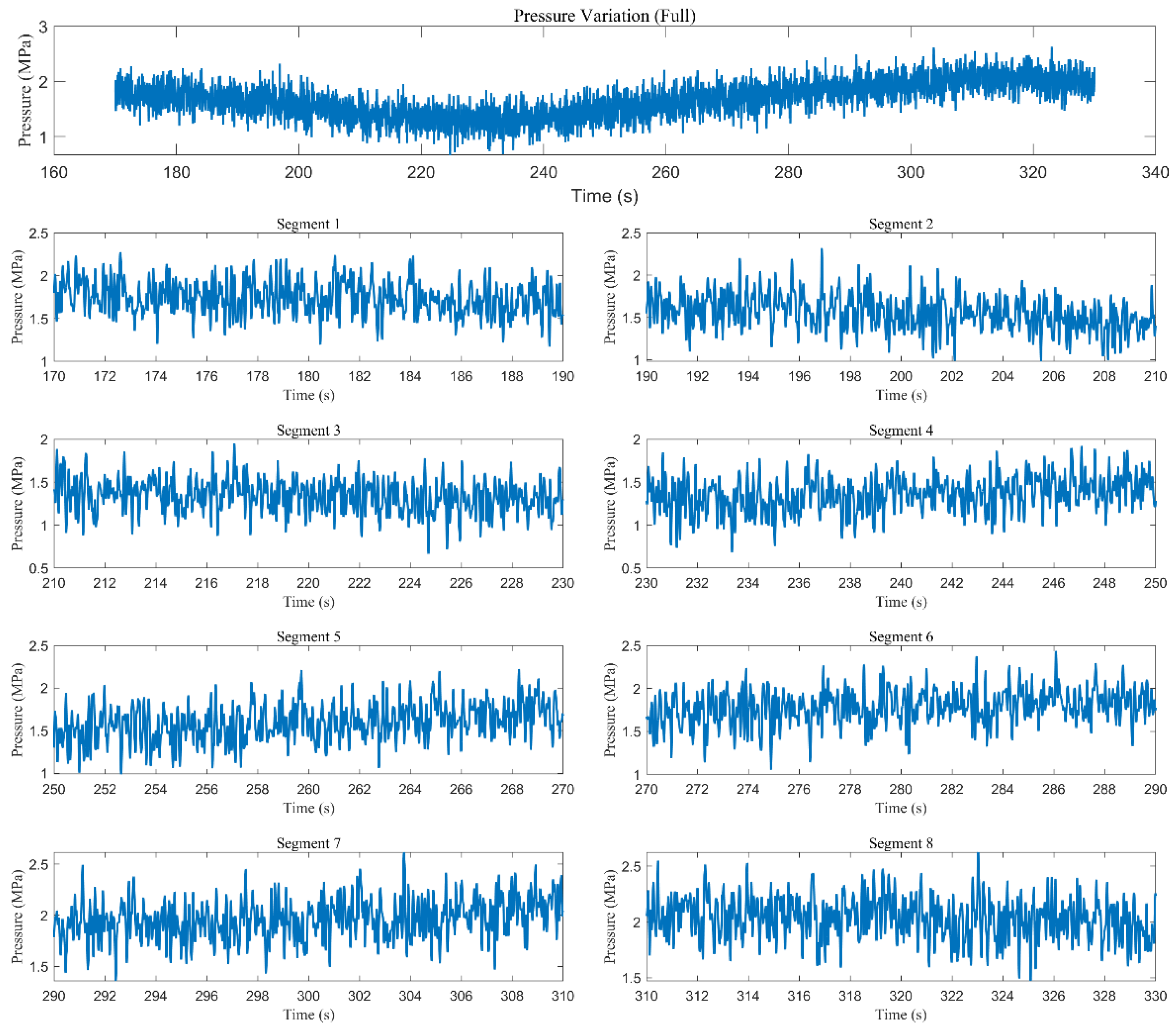
According to the simulation results, the recorded pressure signal contains noise and pressure fluctuations. The first subplot shows the pressure wave variation corresponding to the label sequence. The remaining subplots represent the pressure data for each of the eight labels. In these label subplots, the rising or falling trend of each pressure wave segment can be clearly observed. Figure 10 shows the pressure wave corresponding to the label sequence “10010000” with a noise intensity of 40 dB.

3.2. Pressure Data Preprocessing

During deep learning model training, normalizing the sample data can effectively improve the convergence speed and accuracy of the predictive model. In this study, the Z-score normalization method is applied to the pressure wave data, as defined by Equation (10). The Z-score normalization effectively mitigates the issue of training imbalance caused by varying pressure amplitudes and is better suited for capturing local temporal features within each pressure segment.

$$x_{norm}={\displaystyle \frac{x-\mu }{\sigma +\epsilon }}$$

(10)

where x is the original pressure sequence segment, μ is the mean of the segment, σ is the standard deviation of the segment, and ε is a very small positive constant added to prevent division by zero.

3.3. Feature Parameter Extraction and Dataset Construction

Since LSTM is a special type of recurrent neural network, it processes and memorizes information sequentially according to the order of input data. At each time step, the input corresponds to the “current observation”, while the state from the previous time step is automatically passed through the internal “memory cell”. Therefore, during LSTM model training, it is sufficient to extract the pressure and edge type values from the sample data. The specific data format is shown in

Table 2. Data sample format.

Run	Time	Pressure	TRUE	Edge Type
1	170	1.79452325928619	1	1
1	170.0016	1.7954920287758	1	1
1	170.0032	1.79626405608942	1	1
1	170.0048	1.79682079579245	1	1
…	…	…	…	…
56	223.6608	1.93431696181047	1	0
56	223.6624	1.93492902106014	1	0
56	223.664	1.93548163851746	1	0
…	…	…	…	…

Note: Run: Simulation run identifier. Time: Time stamp of each sample point. Pressure: Corresponding pressure value at that time. TRUE: Validity indicator of the data (1 = valid, 0 = invalid). Edge Type: Label of the signal transition (0 = falling edge, 1 = rising edge).

, where Run indicates the simulation run number, Time represents the time stamp, Pressure is the pressure wave value at the corresponding time, TRUE indicates whether the current information is valid, and Edge Type denotes the label of the pressure wave signal (rising or falling edge).

To enhance the intelligence of pressure wave signal recognition and waveform generation, constructing a highly reliable and representative dataset is one of the fundamental tasks. As mentioned earlier, each throttle valve control command sequence corresponds to a segment of the pressure wave signal. This pressure wave segment is treated as a single sample, and the known label sequence is saved as the sample label. To address practical needs, the mud pulse modulation system is modeled and simulated, and throttle control command sets are batch-generated using a random function to obtain simulated pressure wave data under various operating conditions. On this basis, combined with the physical characteristics of the signal and the pulse response rules, the data are annotated and filtered to construct a well-structured, accurately labeled machine learning training dataset.

4. Results and Discussion

4.1. Results of Model Training

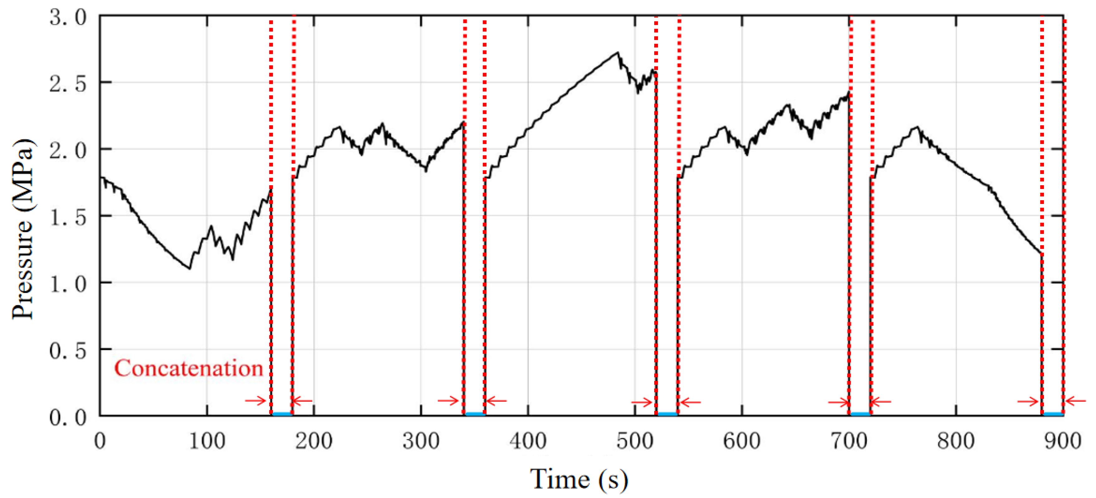
Through multiple simulation cycles of the communication system model, a total of 10,000 sets of pressure wave data were obtained. Since a large number of pressure values correspond to each label during simulation, down-sampling is first applied before training, using an interval of 100 data points. Additionally, to concatenate each complete pressure wave segment, blank segments are inserted between the down-sampled samples. As shown in Figure 11, the length of each blank segment equals the number of pressure points corresponding to one sample after down-sampling. This setup effectively simulates the transmission of continuous commands in real-world scenarios and facilitates data extraction and model training using a sliding window approach.

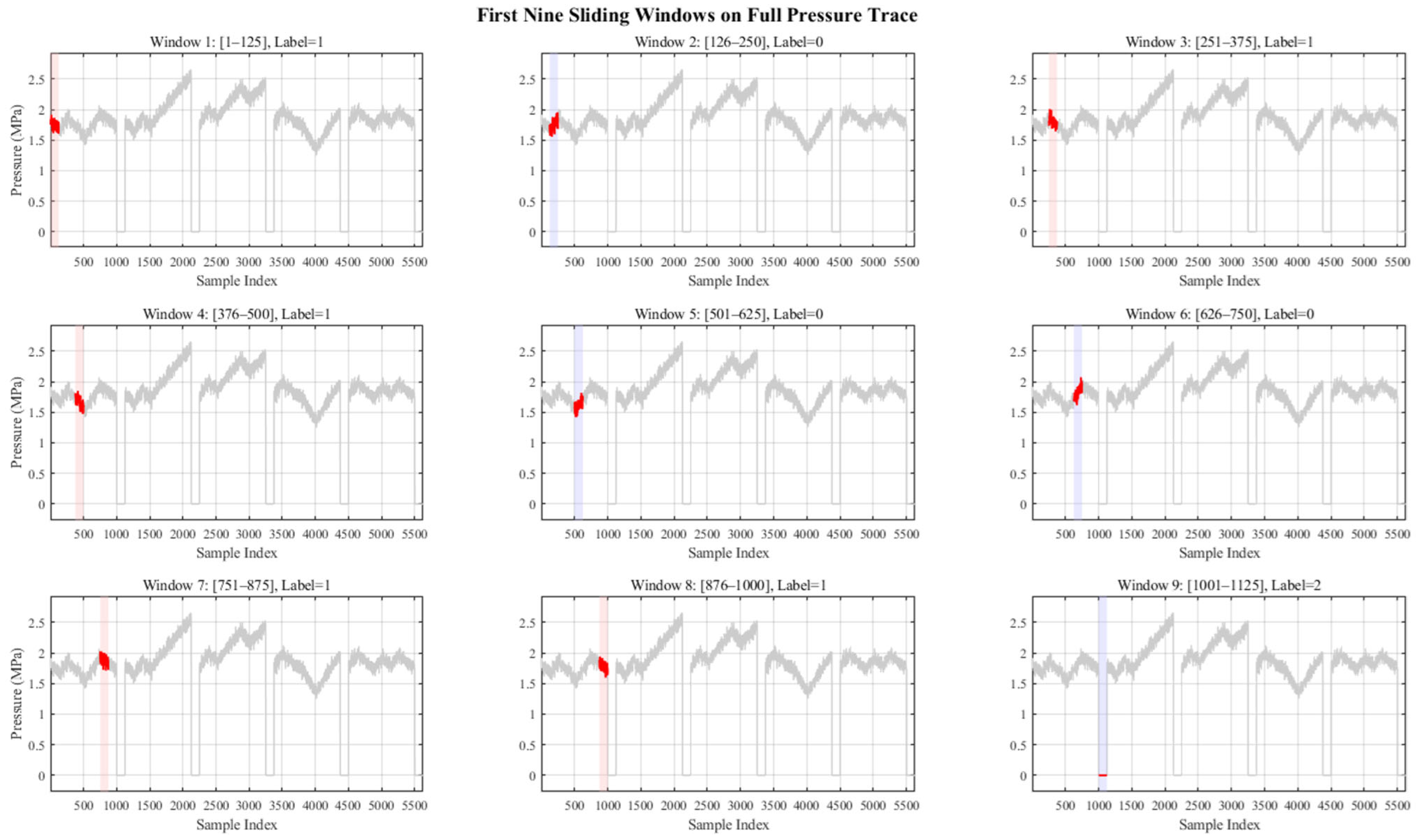
As shown in Figure 12, if the sliding window encounters a blank segment, it will automatically skip that segment to avoid including it in the training process during data extraction. Figure 12 consists of nine subplots in total, illustrating the working process of the sliding window within a complete pressure waveform. In the figure, the sliding window regions are marked in red and blue, where red indicates that the recognized label is ‘1’, and blue indicates a label of ‘0’. The transition segments are denoted by a label value of ‘2’. It is clearly evident from the figure that the sliding window accurately identifies each complete pressure segment corresponding to its label, facilitating effective data extraction and enhancing the model’s prediction performance.

4.1.1. Classifier Training Results

The classifier model structural parameters are shown in

Table 3. Structural parameters of classifier model.

Model	Hyperparameter	Value
LSTM	Layer1	100
	Layer2	50
	Dropout ratio	0.3
	Fully connected layer	2
	Optimizers	Adam
	MaxEpochs	50
	BatchSize	64

below. After down-sampling, each label segment contains 125 pressure data points for a label duration of 20 s. A sliding window of length 1000 (i.e., one complete label segment) is used, with a step size of 125. The validation set ratio is set to 0.2. The classifier achieved a training accuracy of 100%, with perfect classification performance on the validation set.

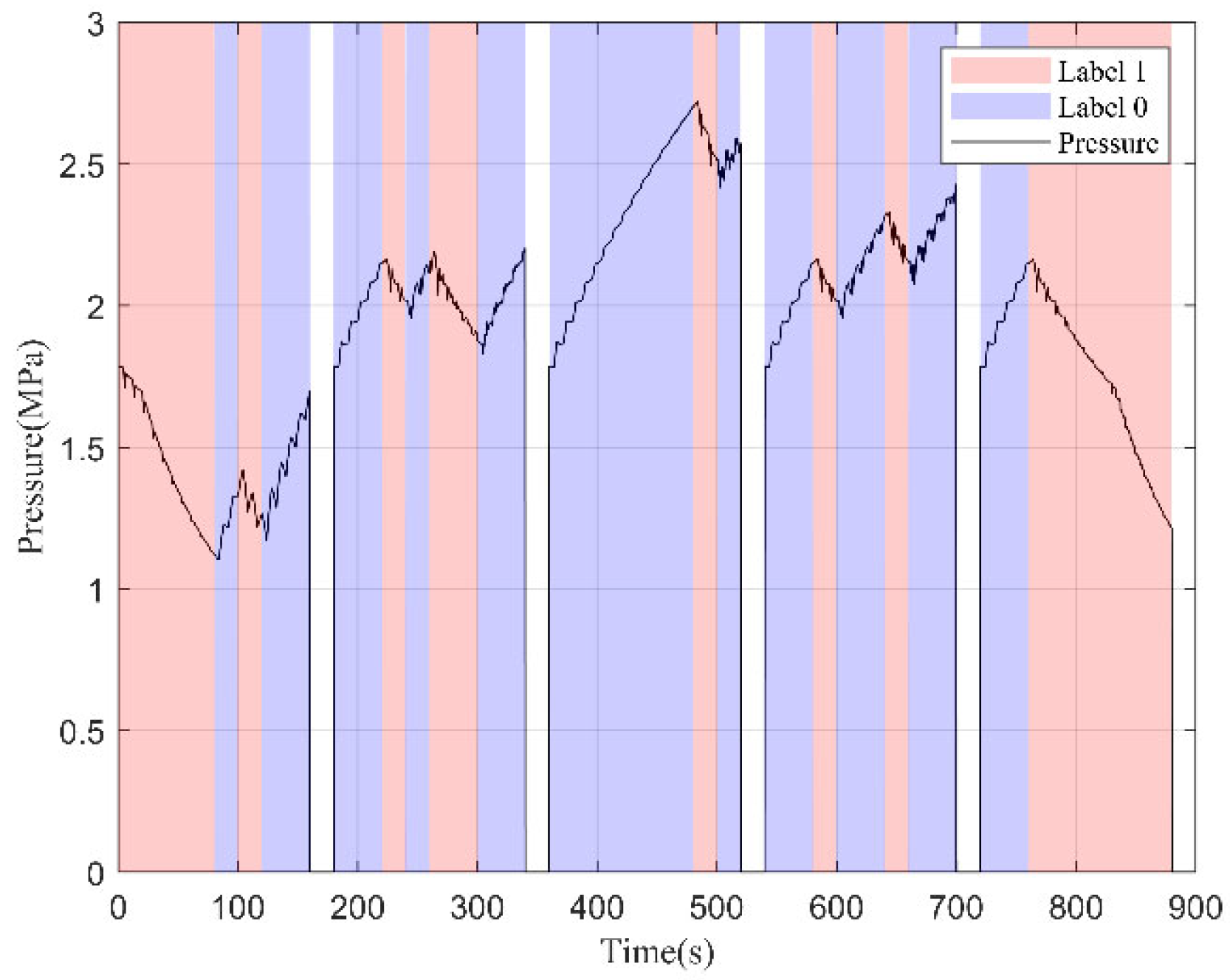
In addition, five pressure wave segments not included in the training dataset were independently generated and fed into the trained classifier for label prediction. As shown in Figure 13, the classifier accurately determines the rising or falling edge based on the pressure wave variation. It clearly distinguishes between rising and falling waveforms and accurately skips over the blank (concatenation) segments. The results demonstrate the high precision and robustness of the classifier.

4.1.2. Generator Training Results

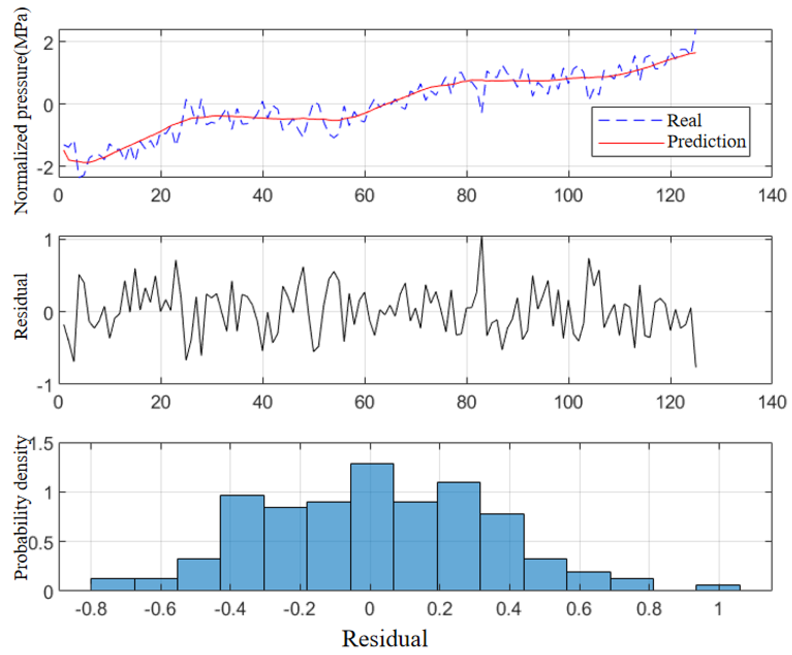
The training parameters for the generator model are based on down-sampled pressure wave data, where each label segment of 20 s corresponds to 125 data points, and there is no noise interference in these data. A sliding window with a step size of 125 is used, and the validation set ratio is set to 0.2. The training results are shown in Figure 14. The proposed dual-channel LSTM generator demonstrates high-precision fitting on normalized pressure waveforms.

In the first subplot, the red predicted curve closely tracks the overall rising and falling trends of the blue ground truth curve, with only a minor lag in small high-frequency fluctuations. The second subplot presents the residual time series, showing that the prediction errors are mostly within ±0.5 and exhibit no apparent systematic drift over time. The third subplot is a histogram of the error distribution, which appears to be nearly symmetric with a peak concentrated in the ±0.2 range, indicating that the errors are random and unbiased.

In terms of quantitative metrics, the model achieves an MSE of 0.1111, MAE of 0.2701, RMSE of 0.3333, and R² of 0.888 on the test set, suggesting that the model can explain approximately 89% of the variance in the pressure wave dynamics. These results further confirm the generator’s strong capability in modeling the temporal behavior of pressure wave sequences.

4.2. Results of Prediction System

By completing the training of both the classifier and the generator, the two models are integrated and invoked according to the system logic shown in Figure 6. The classifier is used to determine the initial label of each complete physical segment (consisting of pressure wave data corresponding to eight labels). The remaining labels of the segment are then inferred by the generator through recursive waveform prediction, followed by residual comparison. This process ultimately yields the full label sequence for each complete physical segment.

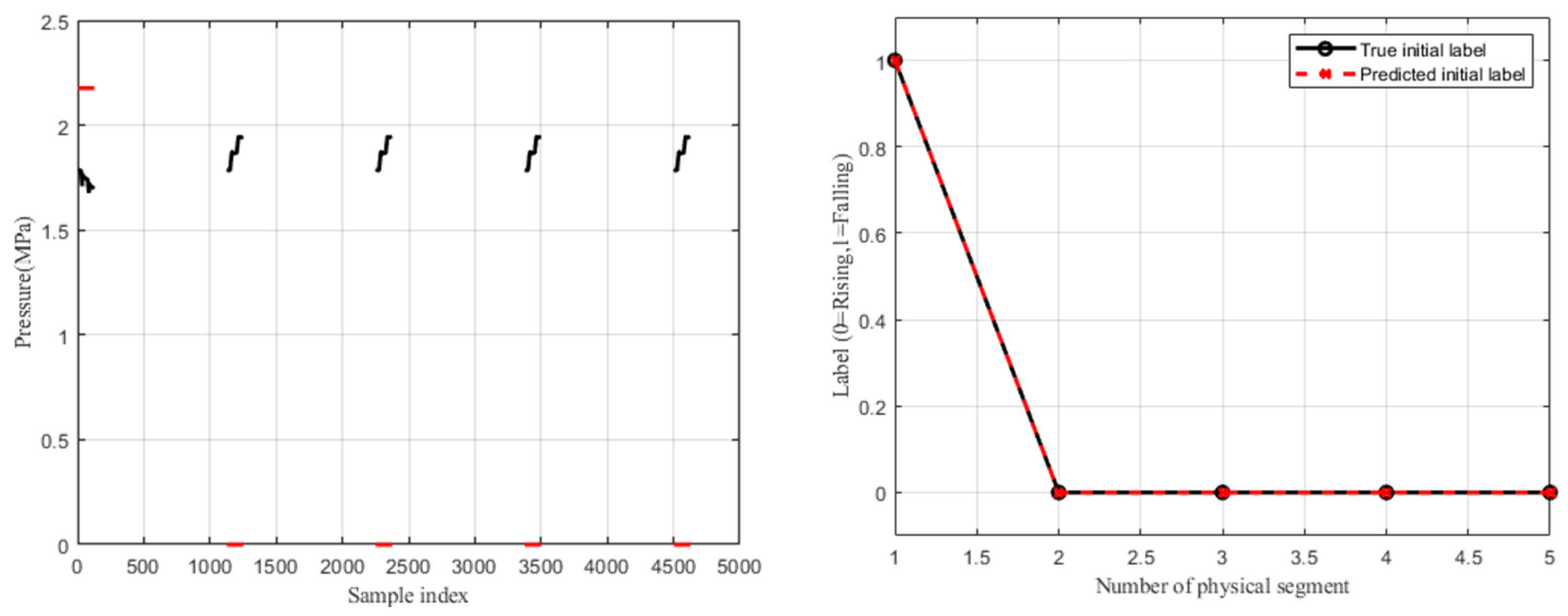
As shown in Figure 15, the left plot displays the waveform of the initial segment of each pressure wave along with the predicted label results. It can be observed that the predicted labels correspond accurately to the waveform trends: a descending waveform is labeled as “1”, and an ascending waveform is labeled as “0”. For the five physical segments, the initial segment trends are as follows: descending, ascending, ascending, ascending, and ascending. The classifier output is “10000”, which is entirely correct.

The right plot presents a comparison between the classifier’s predicted labels for the initial segments and the true labels. The results clearly demonstrate the correctness and reliability of the classifier’s predictions.

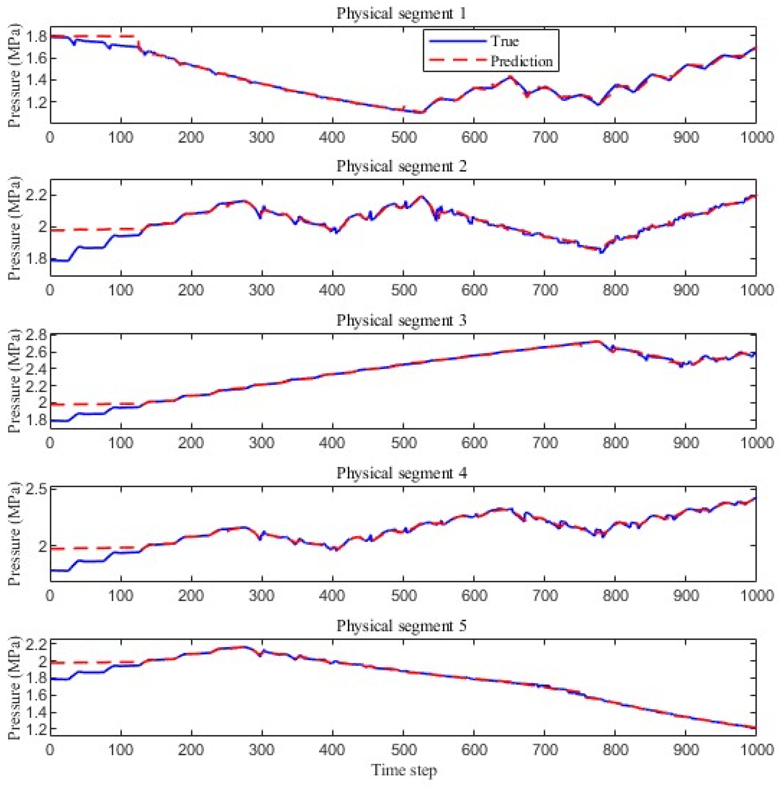
Figure 16 presents the pressure waveforms generated by the generator, comparing the predicted values (red dashed lines) with the actual observed values (blue solid lines). Overall, the predicted curves accurately reproduce the main trends across all physical segments. In the first segment, the rapid pressure drop is precisely captured; the gradual rising trends and turning points in the second and third segments are well aligned with the true signals; and the peaks and troughs in the fourth and fifth segments are effectively fitted.

Although a slight lag is observed in a few high-frequency details—such as the minor oscillation at the end of the second segment—the prediction errors remain within a narrow range, with no evident accumulation or drift. These results demonstrate that the dual-channel LSTM generator not only effectively learns the global dynamics of the pressure waveform but also maintains consistent prediction accuracy and robustness across different segments. This provides a reliable foundation for identifying rising and falling edges in complex pressure wave processes.

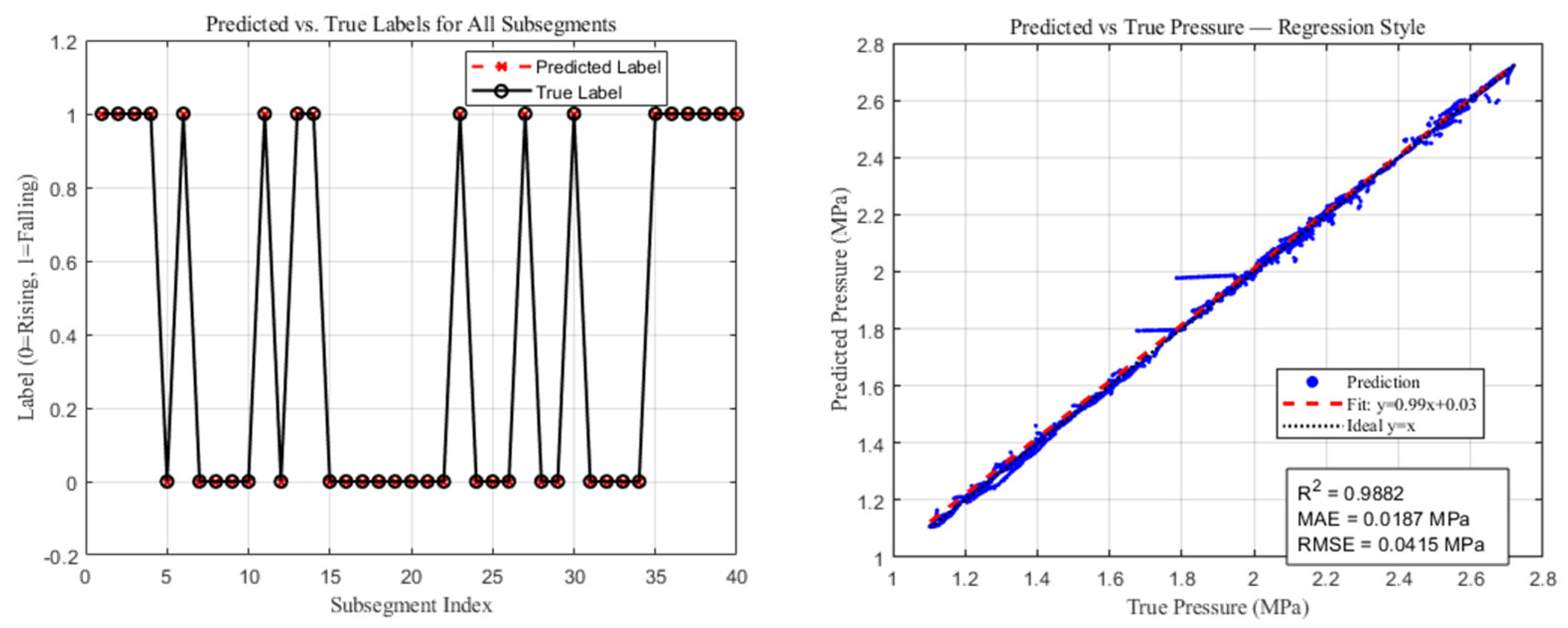
As shown in Figure 17, the red “×” markers (predicted labels) completely overlap with the black “○” markers (true labels) across all 40 subsegments, indicating that the model correctly identifies the rising edges (label 0) and falling edges (label 1) of every segment without exception. This 100% classification accuracy demonstrates the model’s precise edge detection capability within each physical segment—whether the waveform undergoes a gradual transition or a sharp turning point, the model is able to accurately recognize the change, exhibiting outstanding robustness and reliability.

The right plot displays the regression prediction performance of the trained generator model on pressure waveforms. The x-axis represents the true pressure values, while the y-axis represents the predicted values. The blue scatter points denote the prediction outcomes, the red dashed line is the least-squares regression fit, and the solid black line represents the ideal fit y = x. As observed, most points cluster tightly around the ideal line, indicating strong predictive accuracy. The regression equation is y = 0.99x + 0.03, with a slope close to 1, suggesting a high degree of consistency between predicted and true values and minimal bias.

In terms of performance metrics, the coefficient of determination R² reaches 0.9862, meaning the model explains over 98.6% of the data variance. The mean absolute error (MAE) is 0.0187 MPa, and the root mean square error (RMSE) is 0.0415 MPa—both at low levels—further confirming the high accuracy and stability of the model in pressure wave prediction tasks.

4.3. The Impact of Noise on Model Performance

In the previous experiments, the validation set was based on a noise-free environment, where the model demonstrated excellent predictive performance under ideal conditions. To further investigate the model’s performance in environments closer to real-world applications, noise was introduced to simulate practical working conditions [36]. A level of 30 dB corresponds to the typical noise level in a mud pulse channel when the drill bit is operating at high rotational speed and the mud contains a high gas content. A level of 40 dB represents a more favorable condition, such as low-speed drilling with sufficient pulser power and minimal signal attenuation in the channel.

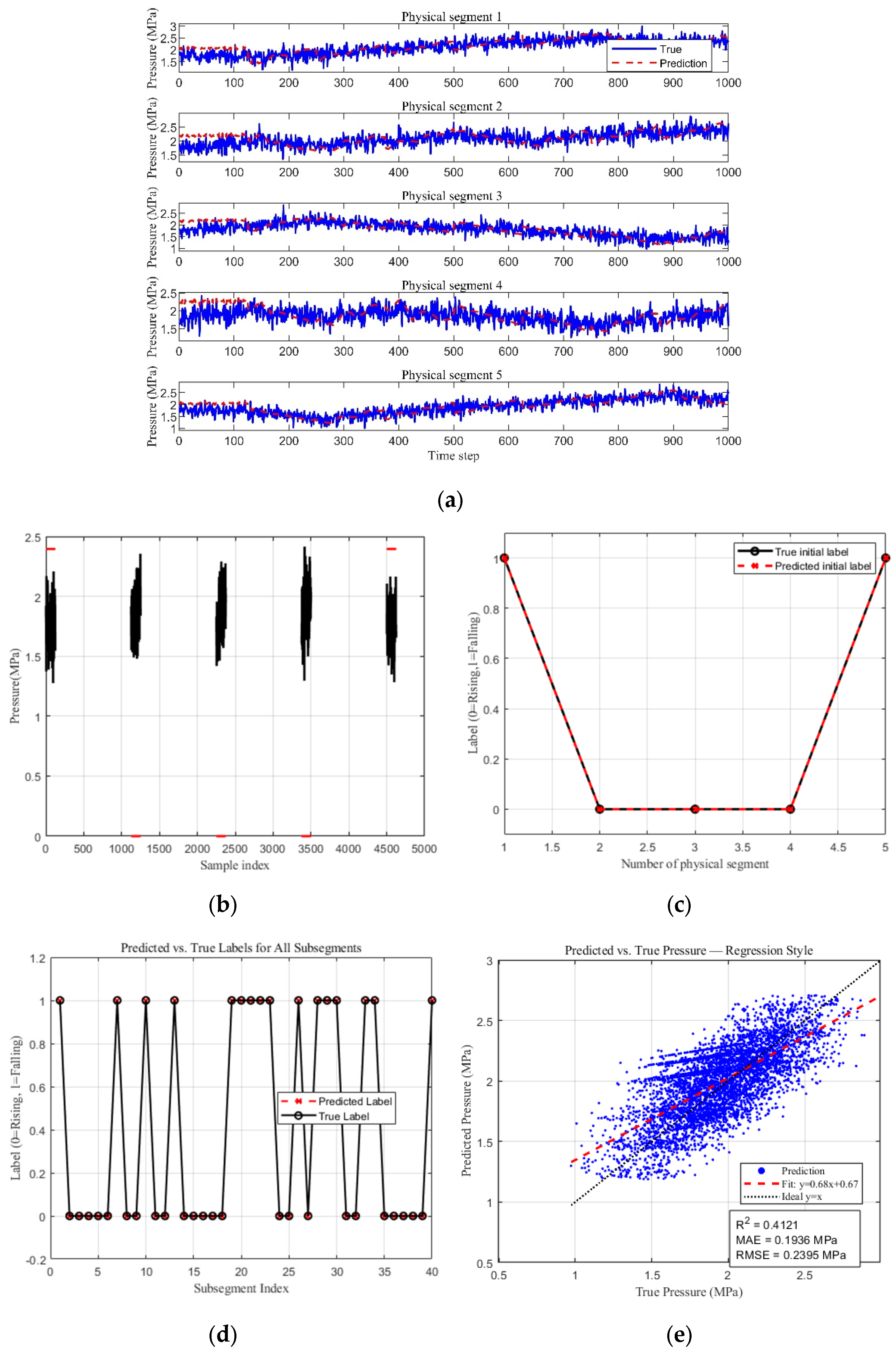
As shown in Figure 18, the five subplots illustrate the model’s prediction results and performance under a noise intensity of 40 dB. From Figure 18a, it can be observed that even with added noise interference, the pressure waves generated by the generator still closely match the actual pressure wave curves. Figure 18b–d presents the label prediction results of the model. It can be seen that under this condition, the model achieved a prediction accuracy of 100%.

Figure 18e shows that the predicted values (blue scatter points) align well with the true values overall. The fitted regression line is y = 0.68x + 0.67, indicating that the model maintains a consistency in prediction trends even under high-noise conditions. Compared to the ideal line, there is a noticeable offset, indicating that the model’s stability slightly decreases under extreme noise conditions.

In terms of fitting precision, the coefficient of determination R² reaches 0.4121. Regarding error metrics, the Mean Absolute Error (MAE) is 0.1936 MPa, and the Root Mean Square Error (RMSE) is 0.2395 MPa. These results indicate that under high-noise conditions, the overall recognition and prediction performance of the model have not completely failed, as the label identification remains accurate. This suggests that the rising and falling edges of the pressure wave can still be correctly detected. However, the performance metrics reveal that the accuracy of the generated continuous waveform is low, indicating a reduced waveform generation capability in noisy environments. This may be attributed to the fact that the model was trained on noise-free data, implying that its noise robustness still needs to be improved.

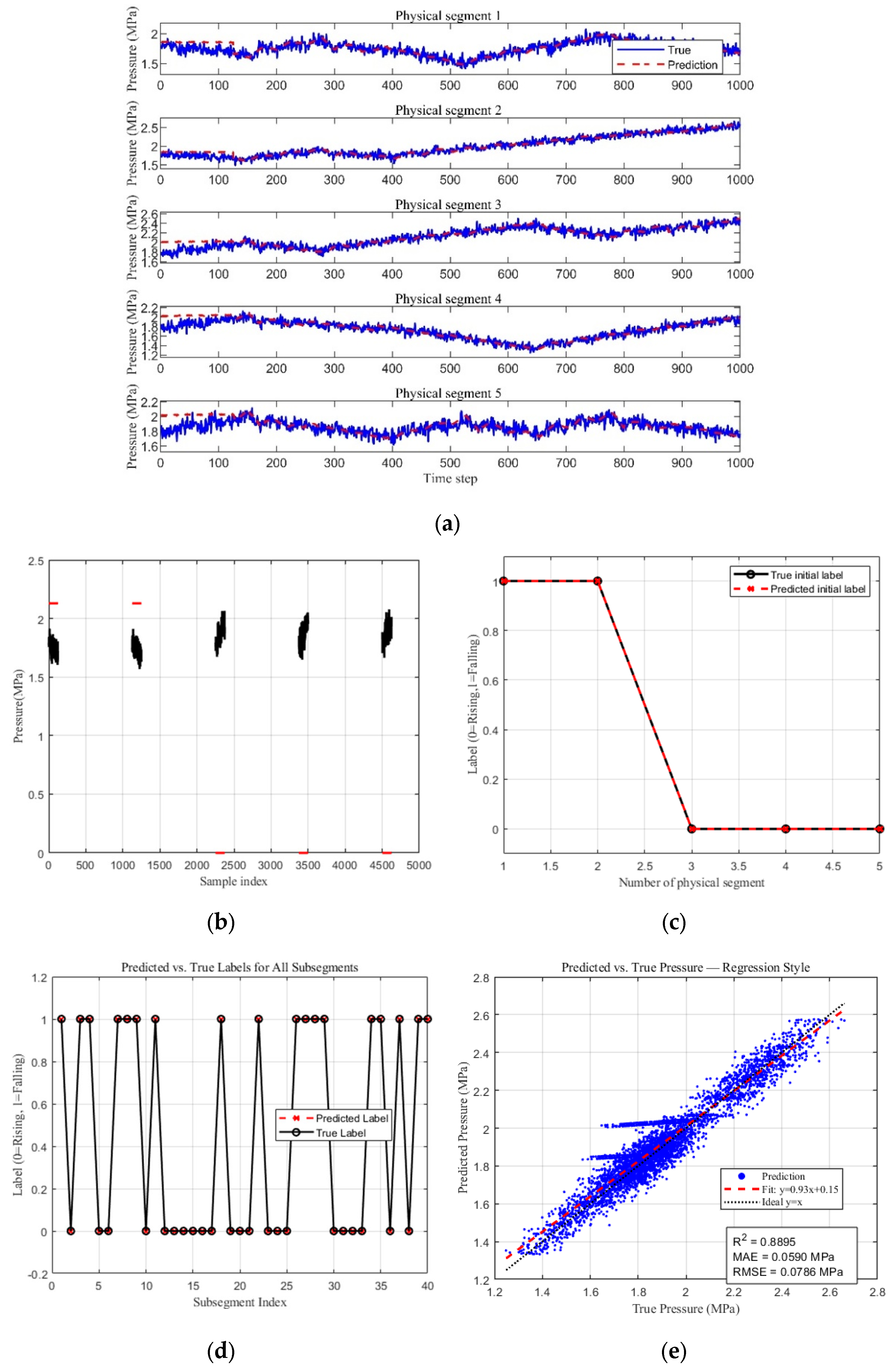
Under a noise intensity of 30 dB, the model’s prediction results and performance are shown in Figure 19. From Figure 19a–d, it can be observed that the model still maintains a high prediction accuracy of 100%. In Figure 19e, despite the significant increase in noise, the generator model continues to demonstrate a good overall consistency in trend. The blue scatter points represent the predicted values, which are mostly distributed along the ideal fit line y = x; however, the enhanced noise leads to a more dispersed point distribution.

The red dashed line is the least-squares regression line, with the fitted equation y = 0.93x + 0.15. It shows that the predicted values (blue scatter points) align well with the true values overall. The coefficient of determination R² = 0.8896 shows that the model still explains approximately 88.96% of the data variance, maintaining relatively strong fitting capability. In terms of error metrics, the MAE is 0.0590 MPa, and the RMSE is 0.0786 MPa, both of which have decreased, suggesting that the model’s prediction accuracy is affected under high-noise conditions. Nevertheless, the overall performance remains within an acceptable range.

In summary, the combined classifier–generator model is capable of accurately identifying pressure wave information even in noisy environments.

4.4. Case Validation

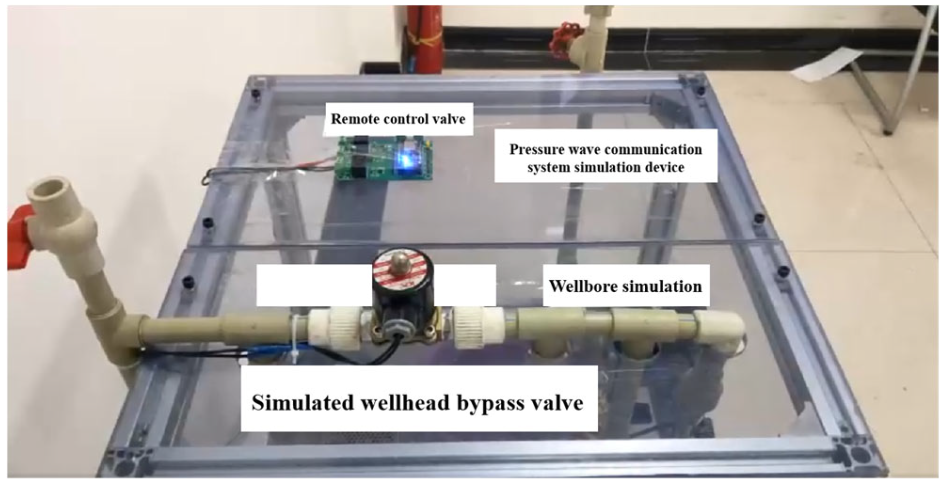
To evaluate the performance of the trained machine learning model under real-world operating conditions, an experimental setup was constructed as shown in Figure 20 to simulate the propagation of pressure waves in a wellbore environment, and the figure presents the top view. The experimental model consists of a simulated wellbore section, a pump, and a remote-control valve used to generate pressure pulse signals corresponding to predefined binary codes. Pressure sensors are installed at key locations along the pipeline to collect real-time data during operation. This setup enables the controlled generation and acquisition of pressure waveform data, providing reliable input for evaluating the prediction accuracy and classification performance of the trained model. By comparing the model’s predictions with actual measurements, the generalization ability and robustness of the model in practical downhole communication scenarios can be effectively assessed.

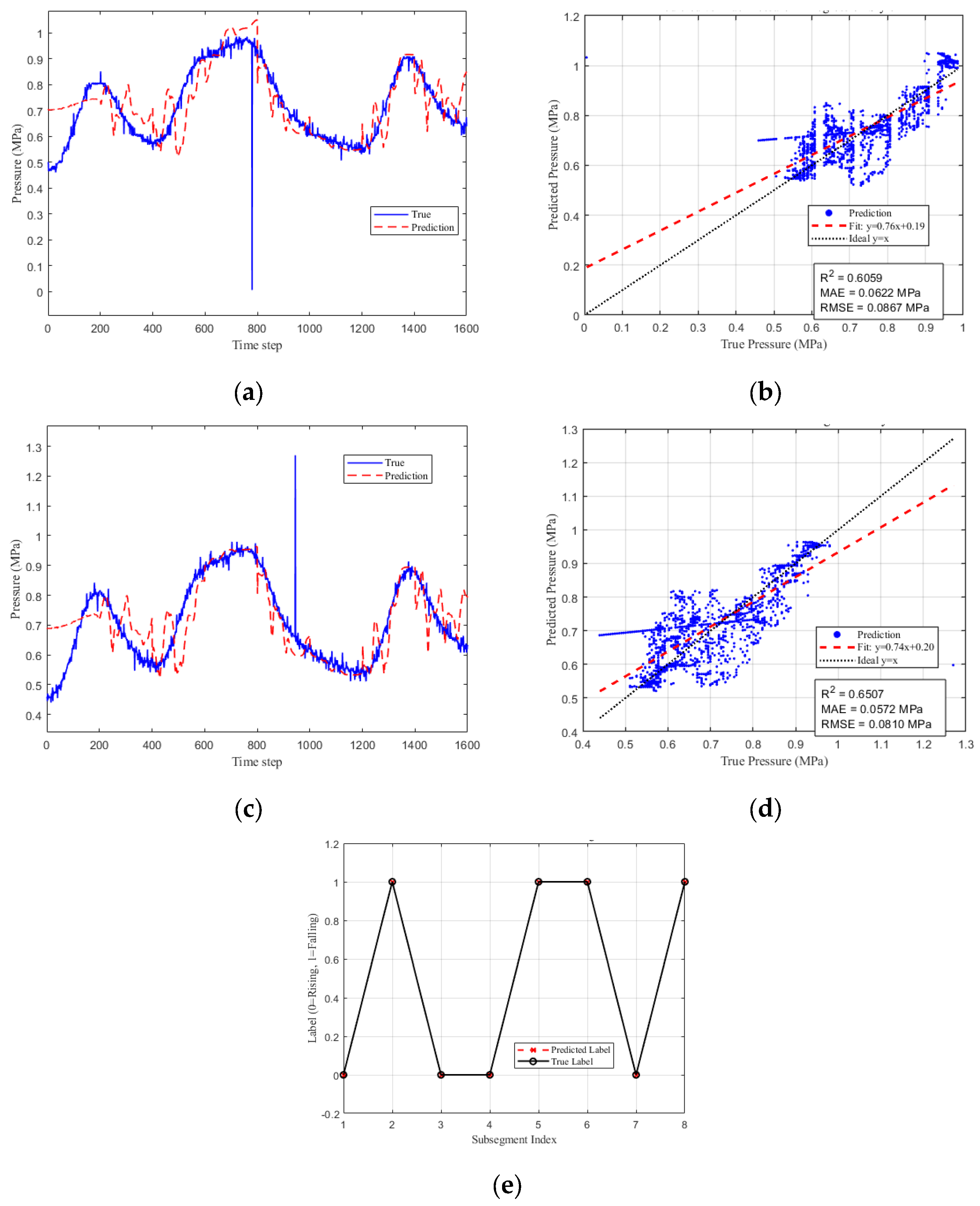
Figure 21a,b, as well as Figure 21c,d, correspond to two different batches of experimental data, both using the same preset binary code “01001101”. Figure 21a,c shows the comparison between the predicted and true pressure values for each batch, while Figure 21b,d presents the corresponding regression performance metrics. The results indicate that even in the presence of real-world noise, the generator is able to fit the pressure waveforms well, and the model performance is not significantly affected by interference.

As shown in Figure 21e, the model successfully identifies the correct labels in both batches, achieving accurate classification. The regression metrics in Figure 21b,d indicate that the model maintains strong predictive performance under experimental conditions, with R² values of 0.6059 and 0.6507 for the two batches and low RMSE and MAE values. These results confirm the model’s generalization ability and robustness when applied to real downhole downlink pressure waveforms.

4.5. Broader Context, Limitations, and Future Outlook

The primary innovation of this study lies in the design and validation of a dual-model LSTM framework specifically tailored for the complex task of downhole pressure wave decoding. While traditional machine learning methods such as SVM or Random Forest often struggle with the long-term temporal dependencies and nonlinearities inherent in these signals, the proposed method achieves 100% label prediction accuracy even under noisy conditions, representing a notable advancement for this specific application. Nevertheless, a key limitation of the current approach is its reliance on supervised learning, which requires large, accurately labeled datasets. In real-world industrial scenarios, generating such datasets is frequently a significant operational and financial bottleneck. This challenge is not unique to downhole communication but is a common obstacle in applied industrial AI. Future research should therefore aim to mitigate this dependency, drawing inspiration from emerging studies in other domains, for instance, threshold-free and label-free pipelines developed for adaptive pulse classification of complex industrial signals [37].

The immediate impact of this work is a validated, practical solution for advancing cable-free measurement-while-drilling (MWD) and intelligent sliding sleeve control in the oil and gas industry. However, the methodology and principles demonstrated here are highly generalizable. The core task—extracting meaningful signals from noisy, dynamic, and physically constrained environments—is fundamental to many high-value industrial processes. Comparable data-driven signal analysis strategies have proven essential for in-process quality control and monitoring in advanced manufacturing. A direct example is found in laser powder bed fusion (LPBF), where such approaches have been applied to identify acoustic emission source motion and positioning effects from sensor data, enabling real-time fault detection and process optimization [38]. These parallels suggest that the proposed framework could be adapted to a wide range of applications, including industrial robotics, structural health monitoring, and non-destructive testing.

Beyond improving predictive accuracy, the next frontier in deploying AI for critical industrial systems such as downhole control is ensuring trustworthiness and interpretability. The current LSTM model, although effective, functions as a “black box” limiting operators’ ability to understand the reasoning behind its predictions. In high-stakes environments, where decisions may have significant safety and financial implications, this lack of transparency is a major barrier to adoption. Future iterations of the framework should therefore incorporate explainable AI (XAI) techniques to address this gap.

A comprehensive XAI strategy—successfully demonstrated in other complex industrial processes—would combine both global and local model inspections. For instance, in the development of data-driven models with physical interpretability for real-time cavity profile prediction in electrochemical machining [39], global inspection methods such as SHAP have been used to identify the most influential signal features (e.g., average pressure, rate of change), aligning model logic with established domain expertise. Concurrently, local inspection methods such as Grad-CAM have been applied to examine model focus on specific time-series segments, revealing its decision-making process during different operational phases and facilitating anomaly detection.

Applying a similar approach in this context could transform the model from a simple classifier into a diagnostic tool. For example, local explanations could pinpoint the segments of a pressure waveform that indicate a sticking valve or interference from reflections. This shift moves the system beyond prediction towards deeper, physically grounded process understanding—akin to how XAI has been applied to identify acoustic emission source motion and positioning effects from complex sensor data in advanced manufacturing [38]. By providing engineers with actionable and interpretable insights, the framework would evolve from a black-box predictor into a trusted diagnostic partner, significantly enhancing its reliability and utility in real-world field applications.

5. Conclusions

This study presents and validates a dual-model LSTM-based framework tailored for signal recognition and waveform prediction in intelligent sliding sleeve downlink communication systems. By simulating the pressure variations induced by throttle valve operations, a high-quality training dataset was constructed. The use of sliding window segmentation and Z-score normalization effectively captured the temporal characteristics of the pressure wave signals.

In the classification stage, the LSTM-based classifier achieved perfect performance, attaining 100% accuracy on the validation set in distinguishing rising and falling edges. For prediction, a dual-input LSTM generator—accepting historical pressure segments and assumed labels—was developed. A residual minimization strategy was employed to iteratively infer the label sequence across each physical signal segment.

To assess real-world robustness, the framework was tested under varying levels of noise (40 dB and 30 dB). Under 30 dB noise, the model maintained good alignment with actual signal trends, achieving an R² of 0.8896, MAE of 0.059 MPa, and RMSE of 0.2395 MPa, while maintaining 100% label prediction accuracy. Even at the more challenging 40 dB noise level, the model retained high predictive accuracy with R² = 0.4121, MAE = 0.1936 MPa, and RMSE = 0.2395 MPa, and the label prediction accuracy also achieves 100%. The model was validated using results obtained from the experimental setup. Although noise interference was present, its impact on the model remained within an acceptable range. Under these conditions, the model achieved R² values of 0.6059 and 0.6507, with relatively low MAE and RMSE values. Validation with real experimental data shows that the proposed prediction method remains effective. However, the process of extracting target pressure wave segments in actual downhole environments still requires further optimization, and the pressure wave data used for training must be properly labeled. Therefore, future work could explore unsupervised learning approaches to reduce reliance on manual labeling.

Overall, the proposed LSTM-based framework demonstrates excellent accuracy and robustness. This study also demonstrates the effectiveness of the LSTM model in decoding downhole communication signals. This approach aligns with trends in other complex industrial domains, where machine learning is increasingly used for prediction and pattern recognition. It provides a solid foundation for advancing cable-free measurement-while-drilling (MWD) systems and remote intelligent sliding sleeve control, offering significant potential for reliable downhole communication in complex drilling environments. Future research could further focus on enhancing the trustworthiness of the proposed framework. Although the current model demonstrates excellent accuracy, incorporating explainable artificial intelligence (XAI) methods can help reveal the underlying decision-making logic, thereby improving its usability and reliability in high-risk industrial scenarios. Such efforts have gained increasing attention in the manufacturing domain, including explainable AI for industrial systems, trustworthy AI in manufacturing processes, and physics-informed data-driven models for real-time cavity profile prediction in electrochemical machining.