Hybrid Model for Medium-Term Load Forecasting in Urban Power Grids

Abstract

In urban power planning, it is typically necessary to predict future monthly, quarterly, and annual electricity consumption to conduct advance planning and ensure the stable operation of the power grid. Therefore, accurate medium-term load forecasting is of critical importance for urban power grid planning and operation. However, current research primarily focuses on short-term forecasting, which is largely limited to a single timescale. To address this issue, this paper proposes a combined model for medium-term load forecasting, enabling predictions of loads over multiple timescales within the next year. This can help optimize power supply planning. First, by improving the 3σ criterion and incorporating holiday corrections, the original data are processed. Combining the advantages of the Prophet algorithm in capturing linear relationships and future trends with the Random Forest algorithm in capturing nonlinear relationships, a Prophet–Random Forest combined forecasting model is constructed. This model is then applied to predict the electricity consumption of a city in southern China. The results demonstrate that the proposed model achieves high accuracy in medium-term forecasting and can predict loads across multiple timescales. Specifically, for annual, quarterly, and monthly predictions, the average prediction errors are 1.02%, 2.66%, and 3.92%, respectively, showcasing strong forecasting performance.

1. Introduction

With the rapid development of urban economies and the continuous growth of the population, electricity demand in urban areas has been steadily increasing [1]. This growth is reflected not only in terms of total volume but also in the increasingly diversified demand structures and more complex consumption patterns. As a result, electricity consumption has become more volatile, posing significant challenges to the safe and stable operation of the power grid [2]. In the power planning of many countries, forecasting electricity consumption for the upcoming month, quarter, and year is essential. This provides a crucial basis for generating power schedules, arranging equipment maintenance and repairs, and optimizing resource allocation [3]. Therefore, accurate load forecasting enables power grid companies to plan effectively for the future, ensuring the safe and stable operation of the grid. Researchers worldwide have conducted extensive and in-depth studies on load forecasting.

Most traditional methods for load forecasting are based on mathematical techniques, such as statistical analysis and time series analysis [4,5]. In reference [6], a cyclic seasonal model was defined, and a linear regression model was constructed based on this model to provide short-term forecasts of hourly electricity consumption in Poland. In reference [7], a short-term load forecast for a park in China was performed using a locally weighted linear regression model. Reference [8] applied grey theory to predict the annual power peak, with the maximum annual prediction error within 5%. Reference [9] developed an autoregressive model to forecast daily and monthly electricity consumption in Greece. Reference [10] proposed the use of a fraction of the optimization based on cuckoo search for the autoregressive moving average (FARIMA) model to perform short-term hourly electricity forecasts in Ireland. As research has progressed, methods such as Markov chains [11,12], Fourier decomposition [13], and Kalman filtering [14,15] have been integrated with time series analysis for load forecasting. The models and algorithms mentioned above are largely based on traditional econometrics and time series analysis. These models are typically simple, with strong interpretability, but they usually perform well only on specific datasets and exhibit poor generalization performance.

In recent years, with the rapid development of computer technology, various artificial intelligence technologies such as machine learning and deep learning have become focal points of research [16]. Reference [17] proposes a hybrid deep learning method combining convolutional neural networks and attention-based seq-to-seq networks, achieving high accuracy in hourly household electricity consumption forecasting in France. Reference [18] proposes a user-behavior-aware machine learning algorithm for real-time residential load demand forecasting. Reference [19] integrates the strengths of Convolutional Neural Networks (CNN), Long Short-Term Memory (LSTM), and Gated Recurrent Units (GRU) to develop a composite model for accurate hourly electricity load forecasting. These algorithms typically rely on large datasets, featuring more complex network structures and computational parameters. While they significantly outperform traditional methods in short-term forecasting, where large datasets are readily available, their improvement in long-term forecasting is less pronounced, with limited gains in accuracy and extended computational time [20,21].

For medium- and long-term forecasting, where data are less abundant and more susceptible to uncertainties, researchers often analyze from the perspectives of data-driven approaches [22,23], trend analysis [24], and external assumptions [25], employing a variety of methods. Reference [26] employed a cointegration approach by postulating three economic growth scenarios to analyze the long-term determinants of electricity consumption and to project China’s electricity demand for the year 2030. Reference [27] considered GDP, population, and other factors, and employed multiple regression and artificial neural networks to forecast annual electricity consumption. Reference [28] employed information feedback mechanisms and system dynamics theory to forecast the evolution of electricity consumption under different carbon neutrality scenarios. Overall, short-term forecasting has benefited from the rapid development of artificial intelligence algorithms based on big data and has achieved high accuracy. In contrast, medium- and long-term forecasting is affected by limited data and uncertainties, resulting in relatively lower prediction accuracy.

Although many algorithms currently achieve high performance in load forecasting, most are limited to a single timescale and struggle to forecast load across multiple timescales [29]. Current research on multi-timescale forecasting predominantly focuses on short-term applications. Most studies incorporate multi-timescale information only at the feature processing stage, while the actual forecasting is still performed at a single timescale [30,31]. Reference [32] generates simulated data based on historical trends and employs machine learning methods with augmented data to forecast both monthly and daily load. Reference [33] analyzes the periodicity and volatility of the load, extracting data features from different timescales and using them to achieve short-term daily and weekly load forecasting. Reference [34] considers seasonal impacts and employs an improved echo state network for multi-scale load forecasting, achieving predictions at the minute, hour, and day scales. Reference [35] processes short-term data into abstract features, which are then concatenated with long-term data to form enhanced feature vectors, and introduces a hybrid neural network architecture that enables ultra-short-term load forecasting (10 min to 1 h) and short-term load forecasting (daily and weekly). Collectively, existing multi-timescale forecasting research remains relatively limited, primarily concentrating on short-term and ultra-short-term load forecasting. Few studies address extended timescales like monthly, quarterly, or annual forecasting.

In addition, for countries such as China, India, and Iran, where holidays follow their own unique calendars, electricity consumption forecasts can be significantly influenced by major holidays [36,37]. For example, in China, electricity consumption in January and February is heavily affected by the Chinese New Year. If this effect is not accounted for in the forecast, the results are likely to be distorted. Reference [38] used historical data to model the relationship between the time interval from the Chinese Lunar New Year to January 1st and the monthly-to-seasonal electricity consumption ratio, thereby adjusting the monthly power consumption for the first quarter. Reference [39] analyzed Korea’s Lunar New Year and applied the Euclidean distance method to identify similar holiday load patterns, and then developed a fuzzy linear regression model to forecast electricity demand during lunar holidays. Therefore, it is necessary to consider the impact of national calendars on electricity consumption data during the forecasting process and make appropriate adjustments to improve forecasting accuracy.

In summary, current mid-term load forecasting for multiple timescales has the following shortcomings: (1) Compared to short-term forecasting, mid-term forecasting is more challenging due to its longer time span. This makes it more difficult to capture the temporal relationship between historical and future data, leading to lower forecasting accuracy. (2) Most existing forecasting algorithms perform well on a single timescale but are not suitable for multi-timescale forecasting, making it difficult to conduct load forecasting across different temporal resolutions. (3) Many studies overlook the potential impact of country-specific calendars on electricity consumption and fail to adequately analyze the relationship between these specific calendars and electricity consumption. To address these issues, this paper proposes an integrated model for mid-term load forecasting in urban power grids, capable of producing forecasts on monthly, quarterly, and annual timescales for the next year.

The main contributions of this paper are as follows:

(1)

By combining Prophet’s ability to capture linear relationships and Random Forest’s strength in exploring nonlinear relationships in the data, the proposed model requires only a small amount of historical data (3–4 years) to achieve high-accuracy load forecasting for the upcoming year.

(2)

The proposed method enables load forecasting across multiple timescales for the upcoming year, including monthly, quarterly, and annual forecasts, all with high accuracy.

(3)

Focusing on China, this paper proposes a correction method for the Chinese New Year holiday. The method adjusts the historical electricity consumption data based on the forecast year, improving forecasting accuracy during the Chinese New Year holiday period.

The rest of the paper is organized as follows: the second part presents the overall framework of the proposed forecasting model; the third part introduces the components of the model; the fourth part introduces the data preprocessing steps, the data correction method for the Spring Festival holiday, and the related evaluation indexes; the fifth part presents two case studies; and the sixth part concludes the whole paper.

2. Predictive Modeling Flowchart

In this paper, a combined Prophet and Random Forest approach is adopted to forecast future electricity consumption. The overall process is illustrated in Figure 1 and consists of the following steps:

(1)

Data cleaning: The raw electricity consumption data are processed using an improved 3σ criterion to identify and remove anomalous values with significant deviations in magnitude. For the removed outliers, as well as for missing values in the original data, cubic spline interpolation is applied to ensure that the interpolated values are consistent with actual conditions.

(2)

Time period segmentation: The available time period T is divided into a historical period T_history and a forecasting period T_future. Correspondingly, the electricity consumption data L are split into L_history and L_future, where L_future represents the target data to be forecasted and L_history is used for forecasting L_future.

(3)

Holiday adjustment: Based on the dates within L_future, the electricity consumption during special periods in L_history (e.g., the Chinese Spring Festival) is adjusted to minimize excessive impacts on the forecasting results.

(4)

Prophet algorithm: The Prophet algorithm is applied to L_history to obtain its fitted values, P_history over T_history, along with the extracted trend, seasonal, and holiday components. These components are then extrapolated to T_future to produce Prophet’s predicted electricity consumption P_future. The series P_history and P_future are combined into P, which is incorporated into the subsequent model training.

(5)

Input–output construction: Using the electricity consumption data L, the Prophet-generated fitted and forecasted data P, and the holiday information H for the corresponding periods, the input and output datasets for the Random Forest model are constructed.

(6)

Random Forest model training: Bootstrap sampling is employed to generate N distinct datasets, each used to build a decision tree as a sub-model. Each sub-model is trained on its corresponding subset and outputs its prediction for future electricity consumption.

(7)

Final prediction and evaluation: The arithmetic mean of the predictions from all sub-models is taken as the final forecast L_forecast for T_future. The accuracy is evaluated by comparing L_forecast against the actual values L_future.

3. Data Adjustments and Evaluation Indicators

3.1. Anomalous Data Cleaning

In machine learning, data quality directly affect the performance of prediction models. In electricity consumption forecasting, manual recording errors, measurement device malfunctions, and other unexpected factors often lead to missing data and anomalies, which pose significant challenges to the training and performance of forecasting models [40,41]. Data cleaning and preprocessing are essential for working with real-world application data.

(1)

Identification of data outliers

Data outliers refer to data points that deviate significantly from the majority of the dataset. The process of identifying such deviations is known as outlier detection. In the field of load forecasting, outliers are often detected using the 3σ criterion, which states that approximately 99.7% of the data should fall within the range of the mean ± three times the standard deviation [42]. Any data points outside this range are considered outliers. However, when the data exhibit a clear monotonic trend and there is a large gap between the maximum and minimum values, identifying outliers effectively using the 3σ criterion becomes challenging. To address this limitation, the traditional 3σ criterion is improved by introducing an exponentially weighted mean.

The formula for the exponentially weighted average is

$$v_i{=\beta v}_{i-1}+(1-\beta )w_i$$

(1)

where $w_i$ is the value of the time series to be processed at point i, $v_i$ is the exponentially weighted average of the corresponding points, $\beta$ is the attenuation coefficient, and the final calculation of $v_i$ is roughly equal to the average of the 1/(1 − β) points before $w_i$. For the initial point, the value is taken as $w_1$, and the subsequent $v_i$ are calculated from the exponentially weighted average. The calculated exponentially weighted average is used to replace the average in the 3σ criterion to identify and eliminate the anomalous data.

(2)

Imputation of missing values

For missing values in the raw data and those arising after the removal of outliers, cubic spline interpolation is used to fill the gaps. Cubic spline interpolation is a commonly used numerical method for approximating and interpolating continuous curves between data points. The basic principle involves segmenting the intervals between neighboring data points and fitting a cubic polynomial function to each segment. This ensures that both the first and second derivatives of the interpolating function are continuous, thereby maintaining the smoothness and continuity of the interpolated curve.

3.2. Correction of Electricity Consumption During the Spring Festival

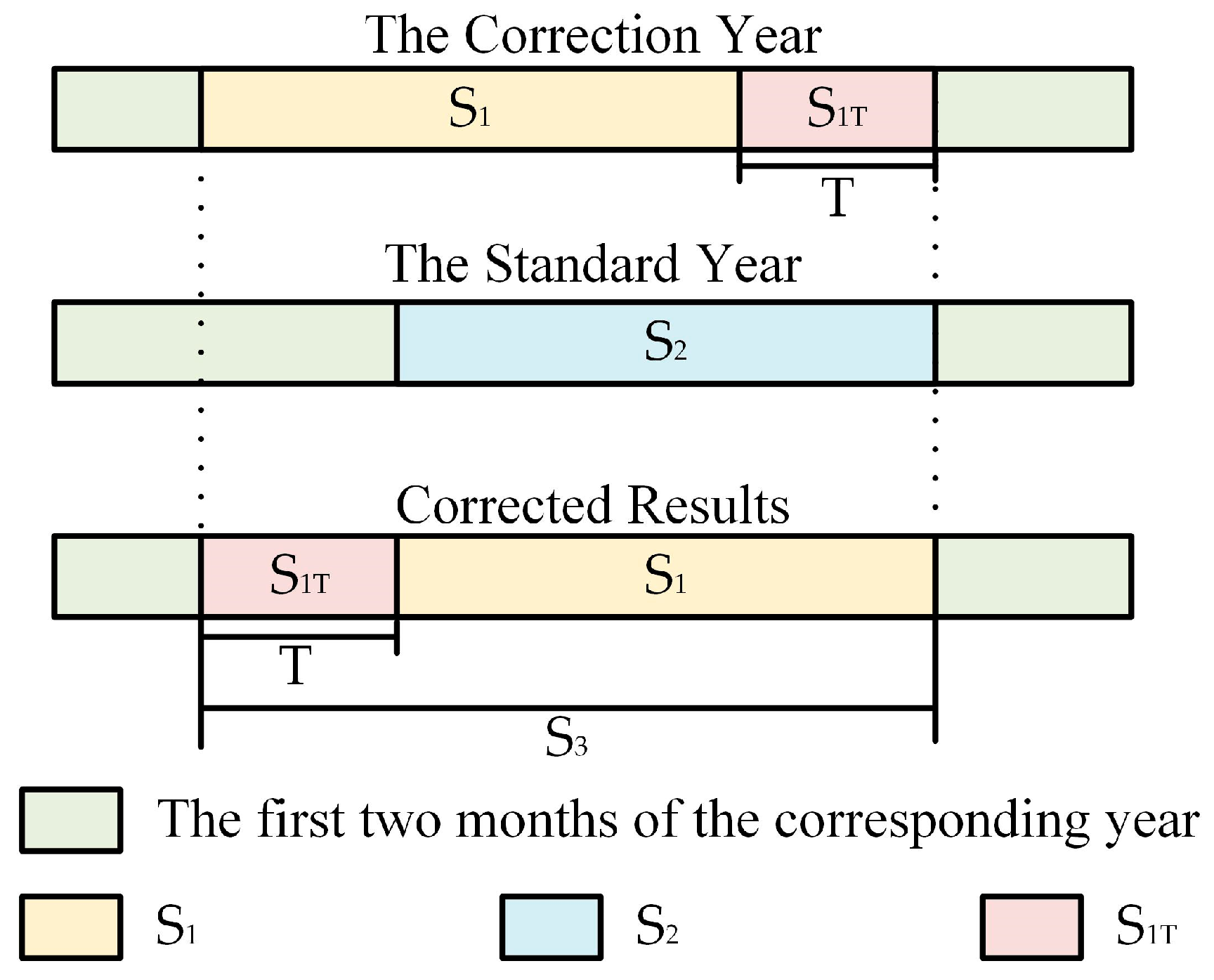
For China, electricity consumption before and after the Spring Festival typically follows a distinct V-shaped distribution. Due to the mismatch between the lunar and Gregorian calendars, the date of the Spring Festival varies each year (typically falling in January or February), which results in significant differences in the proportion of electricity consumption between January and February from year to year. Direct forecasting based on historical data without adjustments leads to significant bias, especially in forecasting electricity consumption for the first two months of each year. Therefore, it is necessary to correct the historical data for the Spring Festival period prior to forecasting. The schematic of this correction process is shown in Figure 2.

The correction is based on the difference in the calendar dates of the Chinese New Year between the forecast year and historical years. The daily electricity consumption in the historical year is adjusted to ensure that the ratio of consumption between January and February aligns more closely with that of the forecast year. This approach effectively corrects the data for the Chinese New Year period.

• We use the forecast year as the reference year and treat each historical year as a correction year, identifying the calendar date of the Spring Festival in each.
• Typically, the 15 days before and after the Spring Festival represent the period most affected by the holiday. These 30-day windows in the correction year and the forecast year are defined as S₁ and S₂, respectively. The union of S₁ and S₂ is defined as S₃, and the date deviation T between the Spring Festival in the correction year and the reference year is calculated.
• Then, the S₁ window is shifted by T days within the S₃. If the shifted S₁ extends beyond the bounds of S₃, the overlapping part (denoted as S_1T) is used to fill in the corresponding missing segment, ensuring continuity. This yields the corrected electricity consumption data for the Spring Festival period.
• After adjusting the electricity consumption as described above, the same correction process is applied to the holiday data.

4. Prediction Algorithms

4.1. The Prophet Algorithm

The prophet algorithm is a time series forecasting model developed by Facebook, specifically designed to handle data characterized by significant trend and seasonal components. It works by fitting long-term trends and recurring seasonal components. With only two to three years of historical data, it can effectively capture the underlying patterns to support forecasting for the upcoming year.

The model can be described as

$$y(t)=g(t)+s(t)+h(t)+\epsilon (t)$$

(2)

where t denotes the moment; y(t) represents the time series to be decomposed; g(t) is the trend component, which captures the non-periodic trend of the time series; s(t) is the seasonal component, which reflects periodic influences; h(t) is the holiday component, which accounts for the impact of specific dates on the time series; and ε(t) is the error component, which is assumed to follow a Gaussian distribution.

A. Trend Component g(t)

The trend component captures the long-term upward or downward trend in a time series. Typically, the Prophet algorithm is fitted with either a segmented linear model or a saturated growth model. In this study, the linear growth model is adopted and can be expressed as

$$g\left(t\right)=\left(k+\mathit{\alpha }{\left(t\right)}^T\mathit{\delta }\right)\times t+\left(m+\mathit{\alpha }{\left(t\right)}^T\mathit{\gamma }\right)$$

(3)

where k denotes the underlying growth rate, m denotes the underlying offset, $\mathit{\alpha }\left(t\right)$ reflects the change in k and m across time intervals, and $\mathit{\delta }$ represents the change in the growth rate across these time intervals.

B. Seasonal Component s(t)

The Prophet algorithm uses a Fourier series to model the seasonal component of a time series, effectively capturing its periodic fluctuations. The seasonal component s(t) with period P has the form of a Fourier series:

$$s(t)={\displaystyle \sum _{u=1}^U\left({\alpha }_{u}cos\left(\frac{2\pi ut}{P}\right){+\beta }_{u}cos\left(\frac{2\pi ut}{P}\right)\right)}$$

(4)

where U denotes the unfolding length, the Prophet algorithm sets a specific U for common cycle steps, and ${\alpha }_u$ and ${\beta }_u$ are both Fourier coefficients.

C. Holiday Component h(t)

The holiday component models the influence of holidays or special dates on the time series. Assuming there are L holidays, let $D_i$ denote the time interval of the i-th holiday, and let ${\kappa }_i$ represent the magnitude of its impact on the time series during $D_i$. The holiday component can then be expressed as follows:

$$h(t)=Z(t)\kappa ={\displaystyle \sum _{i=1}^L{\kappa }_i\times 1_{\left\{t\in D_i\right\}}}$$

(5)

where $Z(t)=\left(1_{\left\{t\in D_1\right\}},1_{\left\{t\in D_2\right\}},\dots ,1_{\left\{t\in D_L\right\}}\right)$, $\kappa ={\left({\kappa }_1{,\kappa }_2,\dots {,\kappa }_L\right)}^T$, and $\kappa =Normal(0{,v}^2)$; the larger the value of v, the greater the impact of holidays on the model.

4.2. Random Forest

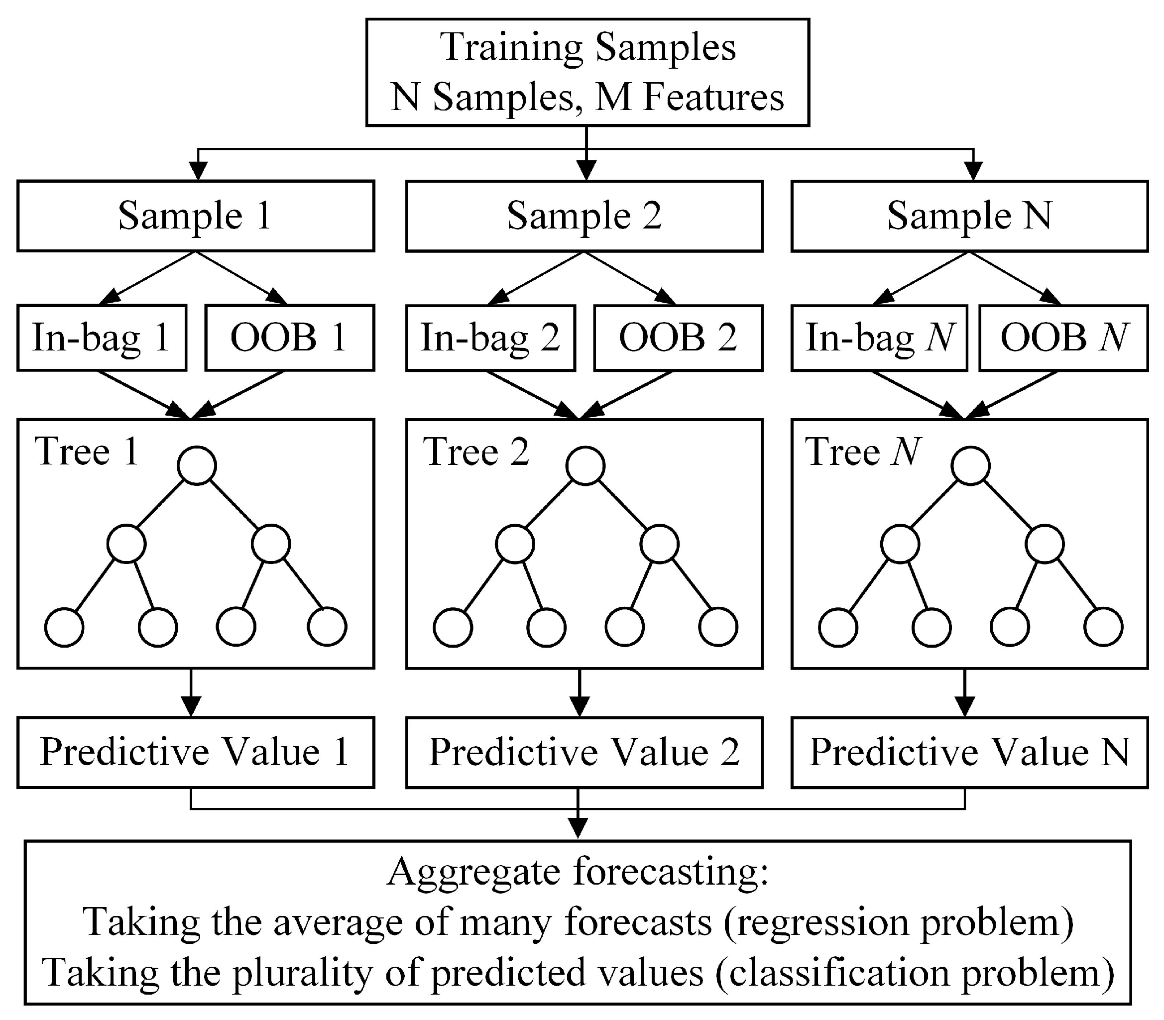
Random Forest (RF), proposed by Breiman in 2001, is a member of the bagging family of methods and one of the earliest ensemble learning algorithms [43]. It excels at capturing nonlinear relationships in data and demonstrates strong predictive performance across a wide range of datasets. Additionally, RF does not require particularly large datasets, unlike algorithms such as deep learning. The RF algorithm can be applied to both regression and classification problems. Since the prediction task in this paper is a regression problem, the Random Forest regression algorithm is used.

RF regression is a widely used nonlinear fitting technique based on regression decision trees. It consists of multiple decision trees and generates predictions by averaging the outputs of individual trees. An RF model containing N decision trees is illustrated in Figure 3.

Its specific process is as follows:

(1)

Each training sample subset is extracted from M features of the original dataset by a self-service resampling technique with put-back random repetitive sampling N times, and N training sample subsets $\left\{{\theta }_1{,\theta }_2,\dots {,\theta }_N\right\}$ are extracted, and each training set can generate the corresponding N regression trees $\left\{{T(x,\theta }_j)\right\},j=1,2,\dots ,N$.

(2)

During the construction of each regression tree, the split points (or nodes) are determined by randomly selecting a subset of the total available variables at each node, rather than considering all the independent variables.

(3)

No pruning is applied to the regression trees, allowing them to grow to their maximum depth.

(4)

All the generated regression trees are combined to form the RF regression model. The final prediction result is obtained by averaging the predictions from all the individual regression trees.

4.3. Forecasting Framework

The Prophet algorithm is effective at capturing trends and seasonality in data, and it performs well even with small datasets. It generates forecasts by linearly summing the trend, seasonal, and holiday components. However, it is less sensitive to nonlinear relationships within the data. In contrast, RF is particularly adept at capturing nonlinear relationships and often exhibits superior performance across various datasets. Additionally, RF does not require a particularly large dataset compared to more complex models like deep learning.

The main advantages of combining the Prophet–Random Forest algorithm for medium-term load forecasting are as follows:

(1)

Minimal data requirements: The algorithm requires relatively little data and can produce accurate predictions with only a few years of historical data.

(2)

Effective trend and seasonality capture: The Prophet algorithm excels at modeling trends and seasonality, while the Random Forest model captures complex nonlinear relationships, thereby enhancing overall prediction accuracy.

(3)

Flexible timescale prediction: The model uses daily data as the minimum prediction scale, allowing it to provide forecasts across multiple timescales, from daily to annual predictions.

In the Prophet model, since urban electricity consumption does not follow a saturating growth pattern, a piecewise linear trend model is adopted. The holiday component is defined based on China’s official holiday calendar, where holidays are assigned a value of 1 and non-holiday days are assigned a value of 0. Additionally, to account for the impact of the COVID-19 pandemic, the holiday component is also set to 1 for the period most affected (20 January to 10 March 2020). The seasonal components considered include annual, quarterly, monthly, and weekly seasonality.

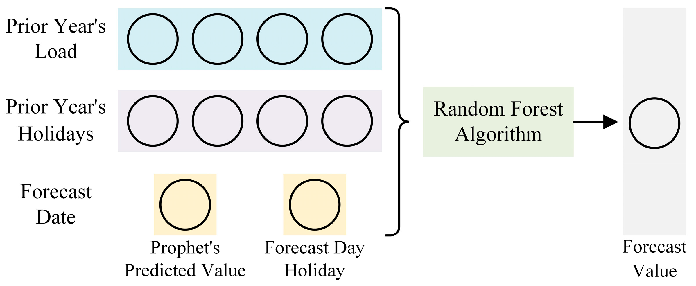
In the Random Forest model, the number of decision trees and the maximum leaf size are determined through parameter tuning, while other parameters remain at their default values. To forecast electricity consumption for the d-th day of a given year, the model uses input features including electricity consumption on days d, d-1, d-2, and d-7 from the previous year, corresponding holiday data, and the Prophet model’s predicted value for day d, as illustrated in Figure 4. During prediction, daily electricity consumption for the target period is predicted and subsequently aggregated to obtain the total forecast.

4.4. Evaluation Indicators

In the context of China’s electricity planning, it is often necessary to forecast the total electricity consumption for the upcoming year, quarter, and month to support timely decision-making and planning. This task falls under medium-term load forecasting, where the focus is on predicting aggregate electricity consumption over these larger timescales, as opposed to daily consumption forecasts.

In this paper, the Prophet–RF algorithm is employed to perform medium-term load forecasting. The approach involves forecasting the daily electricity consumption for each day within the forecasted time span and then summing the predictions to obtain the total electricity consumption for the desired forecasting period. For different timescales, distinct evaluation metrics are adopted.

For the forecasting of total annual electricity consumption, the Absolute Percentage Error (APE) is used as the evaluation metric for this model.

$$\mathrm{APE}=\left|{\displaystyle \frac{S_k{-T}_k}{T_k}}\right|\times 100\%$$

(6)

where $S_k$ and $T_k$ represent the predicted and actual values of total electricity consumption in year k, respectively.

For monthly and quarterly electricity consumption forecasting, the Mean Absolute Percentage Error (MAPE) is adopted as the primary evaluation metric due to the increased number of forecast points at these timescales.

$$\mathrm{MAPE}={\displaystyle \frac{1}{n}}{\displaystyle \sum _{k=1}^n\left|\frac{A_k{-F}_k}{A_k}\right|}\times 100\%$$

(7)

Since APE and MAPE do not reflect the direction of forecasting errors and may produce disproportionately large errors when actual values are small, additional evaluation metrics are employed. These include the Mean Absolute Error (MAE), Root Mean Squared Error (RMSE), R-squared (${\mathrm{R}}^2$), and bias, which provide complementary insights into overall model accuracy.

$$\mathrm{MAE}={\displaystyle \frac{1}{n}}{\displaystyle \sum _{k=1}^n\left|A_k{-F}_k\right|}$$

(8)

$$\mathrm{RMSE}=\sqrt{{\displaystyle \frac{1}{n}}{\displaystyle \sum _{k=1}^n{(A_k{-F}_k)}^2}}$$

(9)

$${\mathrm{R}}^2=1-{\displaystyle \frac{{\displaystyle {\sum }_{k=1}^n{(A_k{-F}_k)}^2}}{{\displaystyle {\sum }_{k=1}^n{(A_k-\overline{A})}^2}}}$$

(10)

$$\mathrm{bias}={\displaystyle \frac{1}{n}}{\displaystyle \sum _{k=1}^n(A_k{-F}_k})$$

(11)

5. Case Study

5.1. Experimental Setup and Software Environment

All data processing and model execution were performed using Python on a Windows 10 system with an Intel Core i7-12700F processor (12 cores, 20 threads) and 32 GB of memory. The experiments were conducted in Python 3.10.13, with key libraries including NumPy (v1.26.4), pandas (v2.1.1), Prophet (v1.1.5), and scikit-learn (v1.4.2). As both Prophet and Random Forest are CPU-based models, GPU acceleration was not required.

5.2. Case Ⅰ

In this case, actual load data of a city in southern China is used, covering the period from 1 January 2019 to 31 December 2023, with daily granularity. Holiday information during the same period was obtained from the Chinese_calendar library (v1.9.0), which provides reliable data on official Chinese holidays. The analysis focuses solely on electricity consumption and holiday data.

For model evaluation, the years 2022 and 2023 are used as test periods. Specifically, to predict the load for 2022, data from 2019 to 2021 are used for training; to predict 2023, data from 2019 to 2022 serve as the training set.

5.2.1. Data Preprocessing

The data analyzed in this paper exhibit a clear upward trend over the years, with significant variations between the lowest and highest electricity consumption each year. To address this, the 3σ criterion is improved by incorporating an exponentially weighted moving average. The results of this improved 3σ criterion for identifying anomalous data are shown in Figure 5.

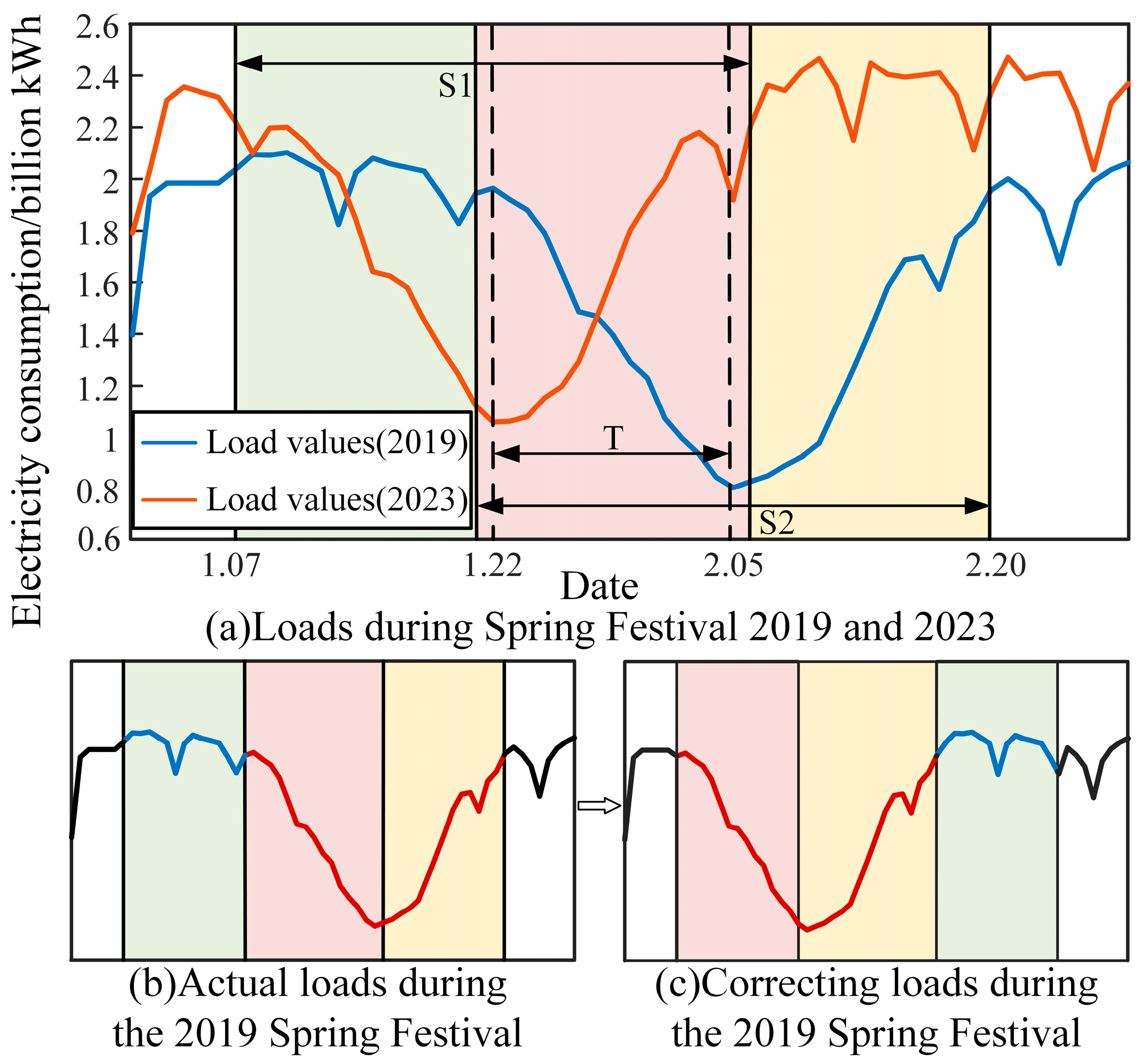
Subsequently, considering the impact of the Chinese Lunar New Year on electricity consumption, the method described in Section 3.2 is applied to correct the historical electricity consumption data, thereby improving the forecast accuracy for the target year. Taking the correction of 2019 as an example for forecasting 2022, the correction results are shown in Figure 6. Although the electricity consumption on individual weekends cannot be fully aligned with specific date types, the correction of the Spring Festival holiday consumption, which has the most significant impact during these two months—effectively enhances the model’s prediction accuracy.

5.2.2. Model Parameter Tuning and Convergence Assessment

In the setup of the Prophet algorithm, seasonal factors generally need to be considered. Previous studies have shown that electricity consumption exhibits strong annual and weekly periodicity and is significantly influenced by factors such as holidays [44,45]. Therefore, in this study, we use the baseline Prophet model that takes into account the annual and weekly seasonality as well as holiday effects. Additionally, the effects of monthly and quarterly seasonality are incorporated by modifying the baseline model, either by adding or removing specific factors, to observe the changes in model performance and assess the impact of each factor on the forecasting model.

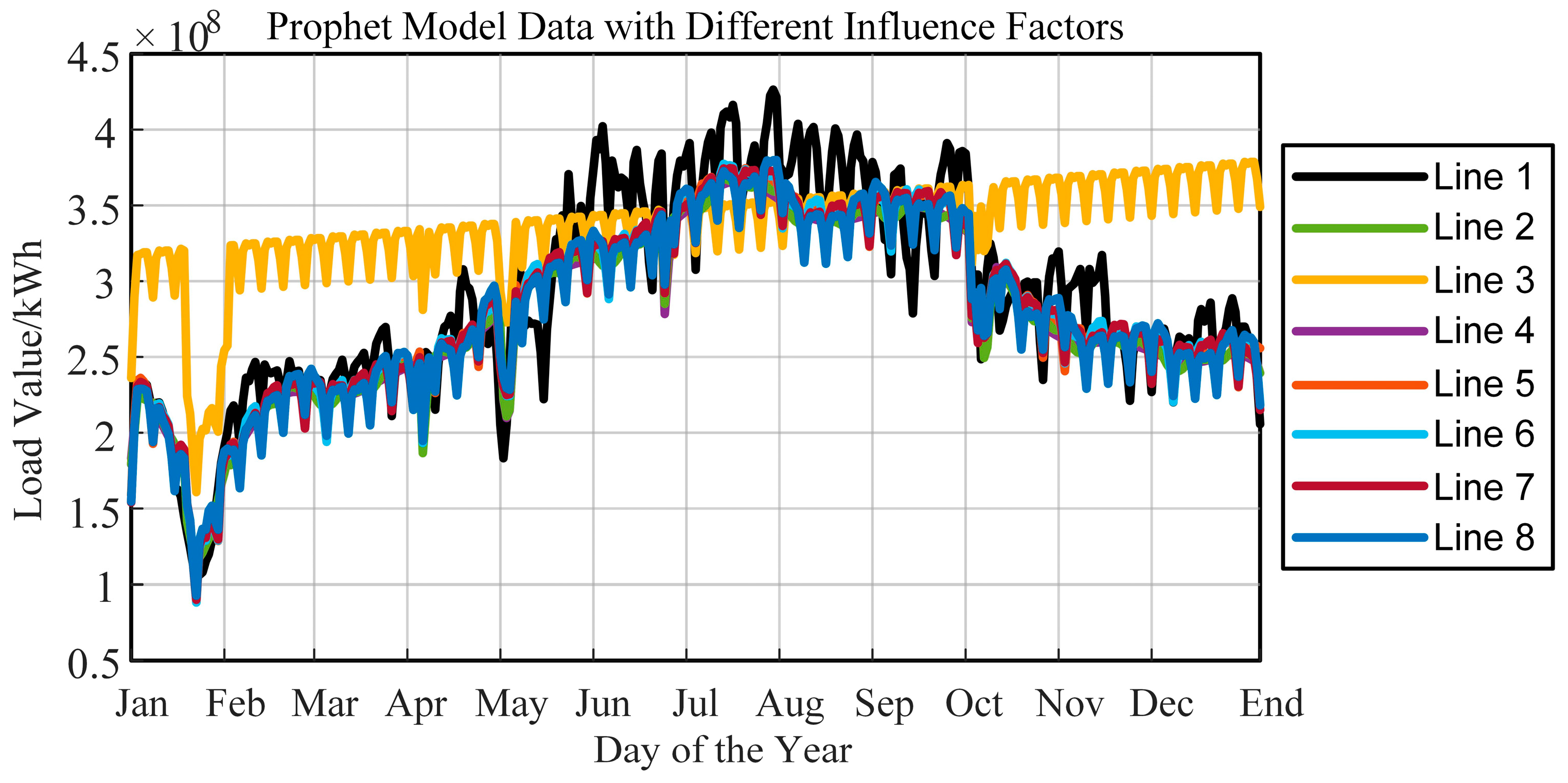
In this case, the Prophet model is trained on data from 2019 to 2022 and used to forecast electricity consumption in 2023. To optimize the model configuration, the effects of various influencing factors are evaluated based on their impact on the 2023 forecasting results. The results obtained by considering different influencing factors are presented in Figure 7.

The comparison of the curves obtained by each model with the actual values is shown in

Table 1. Performance of Prophet model with different influencing factors.

Metric	Line 2	Line 3	Line 4	Line 5	Line 6	Line 7	Line 8
MAPE	6.94	25.30	8.14	9.06	6.87	6.90	7.08
MAE (100 million kWh)	20.4	62.44	24.13	25.85	20.13	20.25	20.58
RMSE (100 million kWh)	25.55	71.83	29.75	31.64	25.38	25.59	25.83
R2	85.91%	−11.35%	80.90%	78.38%	86.10%	85.86%	85.60

.

As shown by the results, under the baseline model that includes annual seasonality, weekly seasonality, and holiday effects, the exclusion of any single component results in a decline in forecasting accuracy. Among these factors, annual seasonality has the most significant influence, as its removal leads to the greatest deterioration in model performance. The effect of annual seasonality is greater than that of holiday effects, which in turn exceed the influence of weekly seasonality. When either monthly or quarterly seasonality is added to the baseline model, forecasting performance improves, with monthly seasonality having a more pronounced effect than quarterly seasonality. However, incorporating both monthly and quarterly seasonality simultaneously leads to a decline in performance, suggesting potential overfitting to the training data. Therefore, when configuring the Prophet model, it is recommended to include holiday effects and to retain seasonality terms for annual, monthly, and weekly patterns to achieve optimal forecasting accuracy.

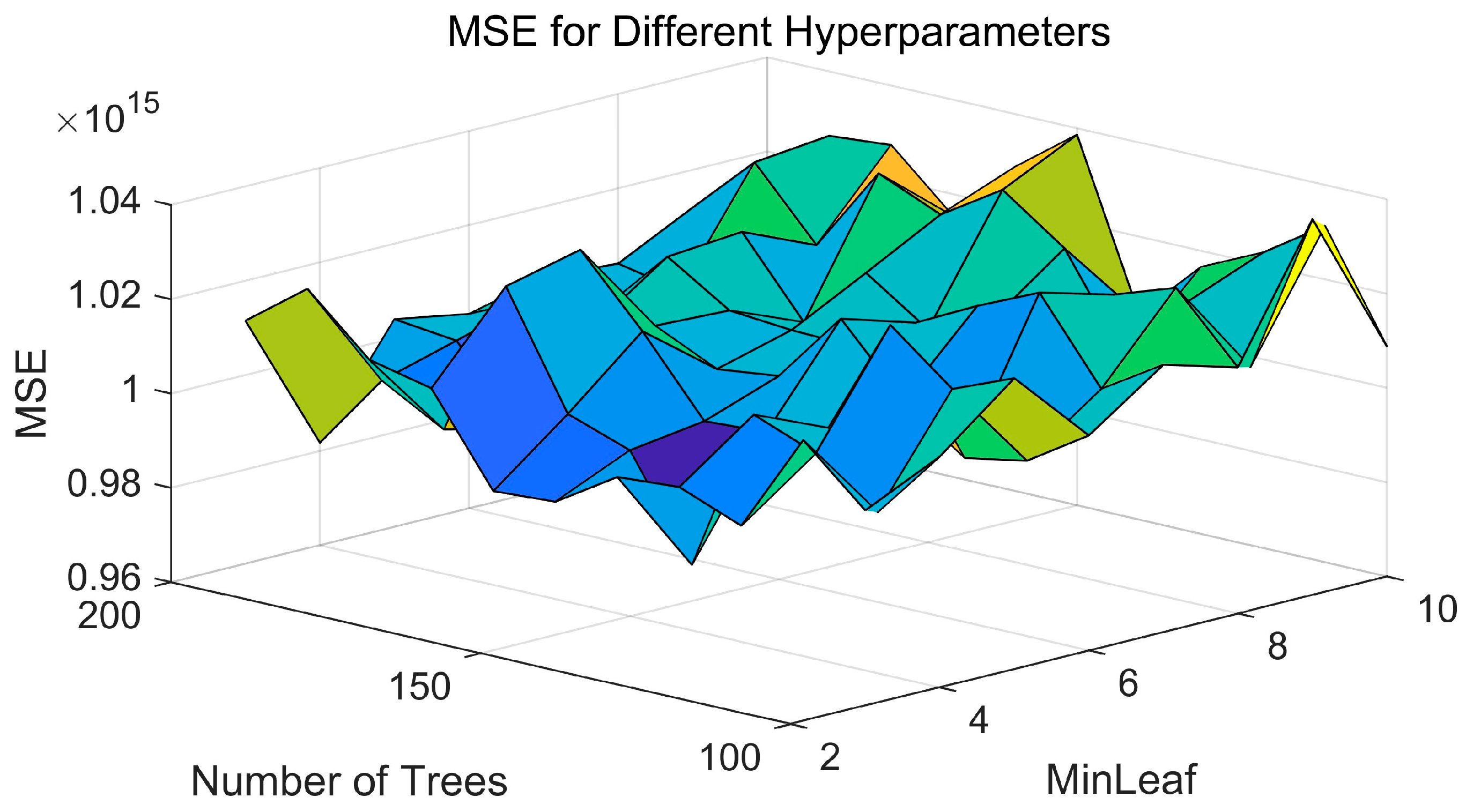
In the training of the Random Forest model, a parameter search approach is considered. According to previous studies, when the number of training samples is relatively small (around 1000), the number of trees can be set to over 100, and the number of leaves can be set between 2 and 10 [43]. Therefore, the parameter search range is set as follows: the number of trees is [100, 110, 120, 130, 140, 150, 160, 170, 180, 190, 200], and the number of leaves is [2, 3, 4, 5, 6, 7, 8, 9, 10]. The case with the smallest Mean Squared Error (MSE) in the test set is chosen as the result for the hyperparameter setting. The final results are shown in Figure 8. When the number of trees is 140 and the number of leaves is 4, the minimum MSE value is achieved. Therefore, these values are selected as the hyperparameters for the Random Forest model.

After setting the model-related parameters, the electricity consumption data for 2022 and 2023 can be predicted and validated.

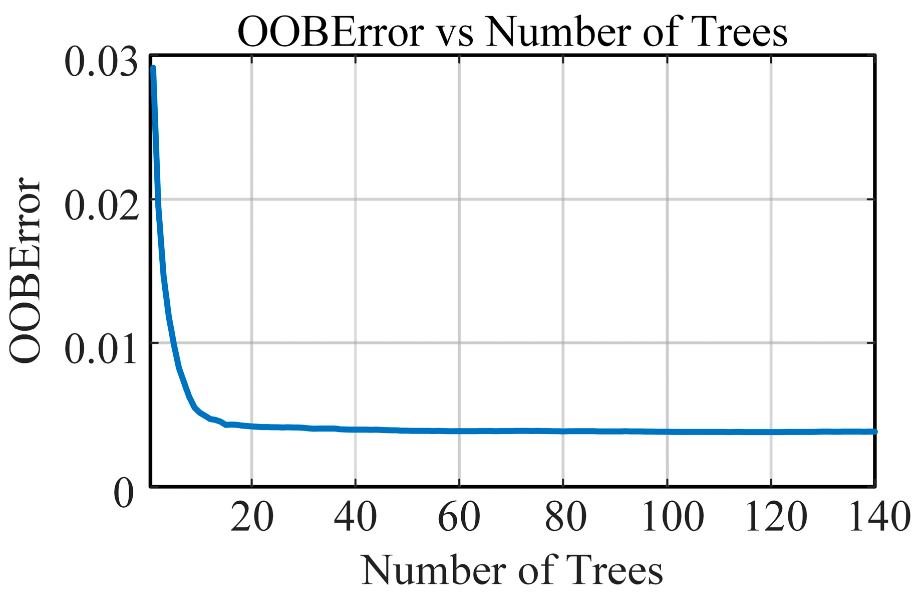
When using the proposed model for forecasting, the Prophet model is a time series forecasting model based on Bayesian regression. It uses a stable algorithm to generate the forecast results. During the fitting process, it does not rely on traditional optimization methods (such as gradient descent) to find the optimal solution, so convergence is not explicitly considered during training. In contrast, Random Forest does not converge through iterations like optimization algorithms such as gradient descent. Instead, it generates a collection of trees by constructing decision trees, and the result is obtained through this ensemble. It typically uses the Out-of-Bag (OOB) error to evaluate the model’s generalization ability. This can also be considered a form of “convergence” testing. When testing with the 2023 data, the OOB error for each tree was plotted, and the results are shown in Figure 9.

It can be seen that as the number of trees increases, the OOB error decreases significantly. After 20 trees, the rate of decline slows down. By the time 60 trees are reached, the OOB error no longer decreases with the addition of more trees, and it stabilizes, indicating convergence. The variation in the OOB error for the 2022 data during testing follows a similar pattern, suggesting that the model has reached a convergent state and can be used for forecasting future electricity consumption.

5.2.3. Multi-Scale Medium-Term Electricity Consumption Forecasts

The data analyzed in this paper exhibit a clear upward trend over the years, with significant variations between the lowest and highest electricity consumption each year. To address this, the 3σ criterion is improved by incorporating an exponentially weighted moving average. The results of this improved 3σ criterion for identifying anomalous data are shown in Figure 5.

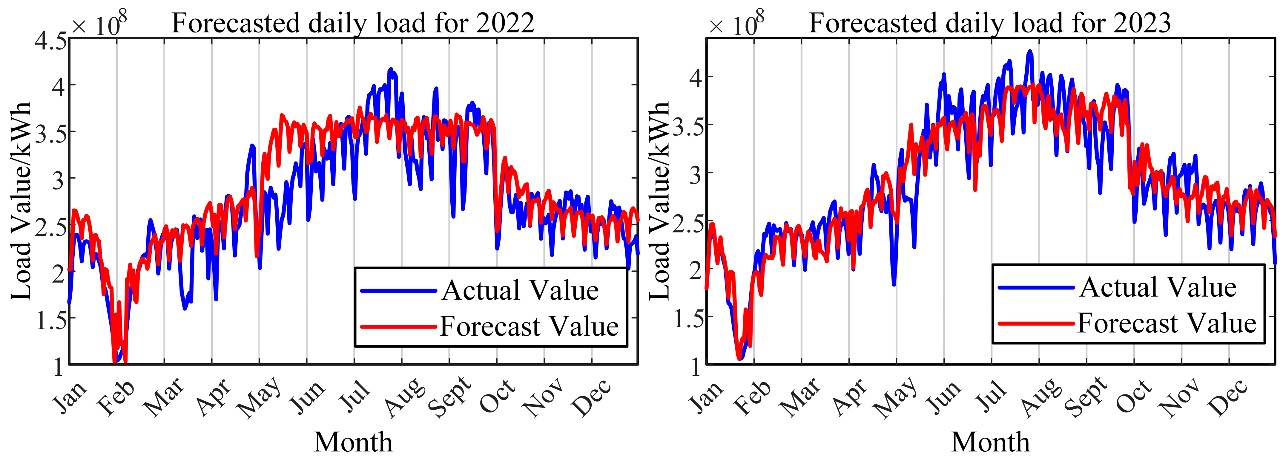
The forecast results for total electricity consumption in 2022 and 2023 using this method are presented in Figure 10 and

Table 2. Forecast results using Prophet–Random Forest (2022–2023).

Year	Evaluation Indicators	Prophet	RF	Prophet–RF
2022	MAPE	9.81	14.26	7.89
	APE	5.67%	9.07%	1.64%
2023	MAPE	6.94	8.96	6.89
	APE	3.80%	3.51%	0.39%

.

It can be observed that for the 2022 forecast, the MAPE is 7.89%, and the total annual error is 1.64%. For the 2023 forecast, the MAPE is 6.89%, and the total annual error is 0.39%. Compared to using either the Prophet or Random Forest algorithm alone, the proposed model achieves lower MAPE values and smaller annual errors. A comparison of this method with several commonly used time series forecasting algorithms is shown in

Table 3. Comparison of predicted values and actual values from different algorithms (Unit: 100 million kWh).

Year	Actual Value	Prophet–RF	Prophet	RF	Cubic Exponential Smoothing	SARIMA	Gray Forecast	LSTM	XGBoost	BiLSTM
2022	1003.05	1019.50	1059.92	1094.03	1068.35	1039.26	1042.57	1083.45	1080.31	1067.42
2023	1060.22	1064.34	1100.51	1023.01	1005.94	1116.62	1108.14	1044.92	1044.39	1046.52

and

Table 4. Comparison of annual electricity consumption data predicted by different models.

Model	2022			2023			Average Runtime
	APE	AE (100 Million kWh)	Error Direction	APE	AE (100 Million kWh)	Error Direction
Prophet–RF	1.64%	16.45	Overestimate	0.39%	4.12	Overestimate	2.41 s
Prophet	5.67%	56.87	Overestimate	3.80%	40.29	Overestimate	1.49 s
Random Forest	9.07%	90.98	Overestimate	3.51%	37.21	Underestimate	1.05 s
Cubic Exponential Smoothing	6.51%	65.3	Overestimate	5.12%	54.28	Underestimate	0.89 s
SARIMA	3.61%	36.21	Overestimate	5.32%	56.4	Overestimate	0.49 s
Gray Forecast	3.94%	39.52	Overestimate	4.52%	47.92	Overestimate	0.22 s
LSTM	8.01%	80.4	Overestimate	1.44%	15.3	Underestimate	8.35 s
XGBoost	7.70%	77.26	Overestimate	1.49%	15.83	Underestimate	0.91 s
BiLSTM	6.42%	64.37	Overestimate	1.29%	13.7	Underestimate	14.51 s

.

From Table 3 and Table 4, it can be seen that the proposed model achieves the best performance in both APE and Absolute Error (AE). Although the Prophet and Random Forest models have simpler structures compared to deep learning models, the computation time required, while slightly longer than traditional models such as Random Forest, Prophet, SARIMA, and XGBoost, is still significantly shorter than that of deep learning models like LSTM. The results can be computed within a few seconds without the need for GPU acceleration, requiring minimal computational resources.

Considering that this model is a daily cumulative model to estimate the annual total, it can also be applied to predict electricity consumption at different timescales, such as monthly and quarterly. By forecasting the daily electricity consumption and summing the predictions accordingly, the model can generate the forecasted electricity consumption for both monthly and quarterly time frames.

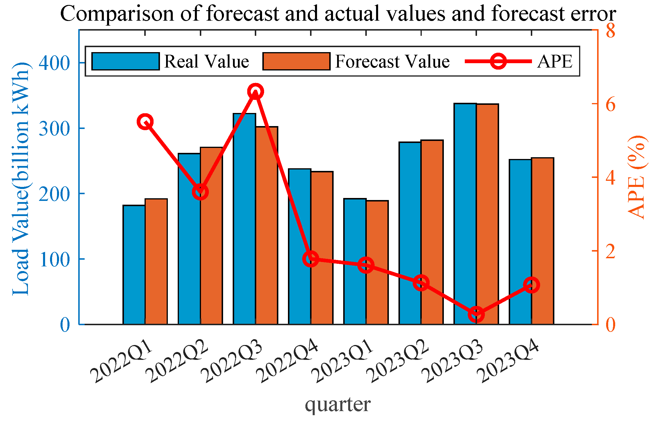
For quarterly forecasting, the results of the forecasts for all four quarters of 2022 and 2023 are analyzed and validated. In each quarterly forecast, the electricity consumption up to that quarter is treated as a known value (for example, when forecasting the second quarter of 2023, the data from the first quarter of 2019 to the first quarter of 2023 are considered known, with the same approach applied for the other quarters). The model construction, inputs, and outputs are identical to those used for annual forecasting. The results of these eight quarterly forecasts are presented in

Table 5. Forecast results of electricity consumption by quarter in 2022 and 2023 (Unit: 100 million kWh).

Period	2022Q1	2022Q2	2022Q3	2022Q4	2023Q1	2023Q2	2023Q3	2023Q4
Real Value	181.85	261.15	322.35	237.70	192.14	278.48	337.66	251.93
Forecast Value	191.88	270.54	301.93	233.47	189.04	281.63	336.74	254.63
APE	5.51%	3.60%	6.33%	1.78%	1.61%	1.13%	0.27%	1.07%

and Figure 11.

It can be observed that for the quarterly forecasts, the overall MAPE value is 2.66%. Except for the first three quarters of 2022, the prediction errors for all other quarters are within 2%. Additionally, since more data are available for training compared to the previous year, the prediction accuracy for 2023 is higher than that for 2022. Overall, the model’s quarterly predictions are relatively accurate, with the overall error staying within 3%.

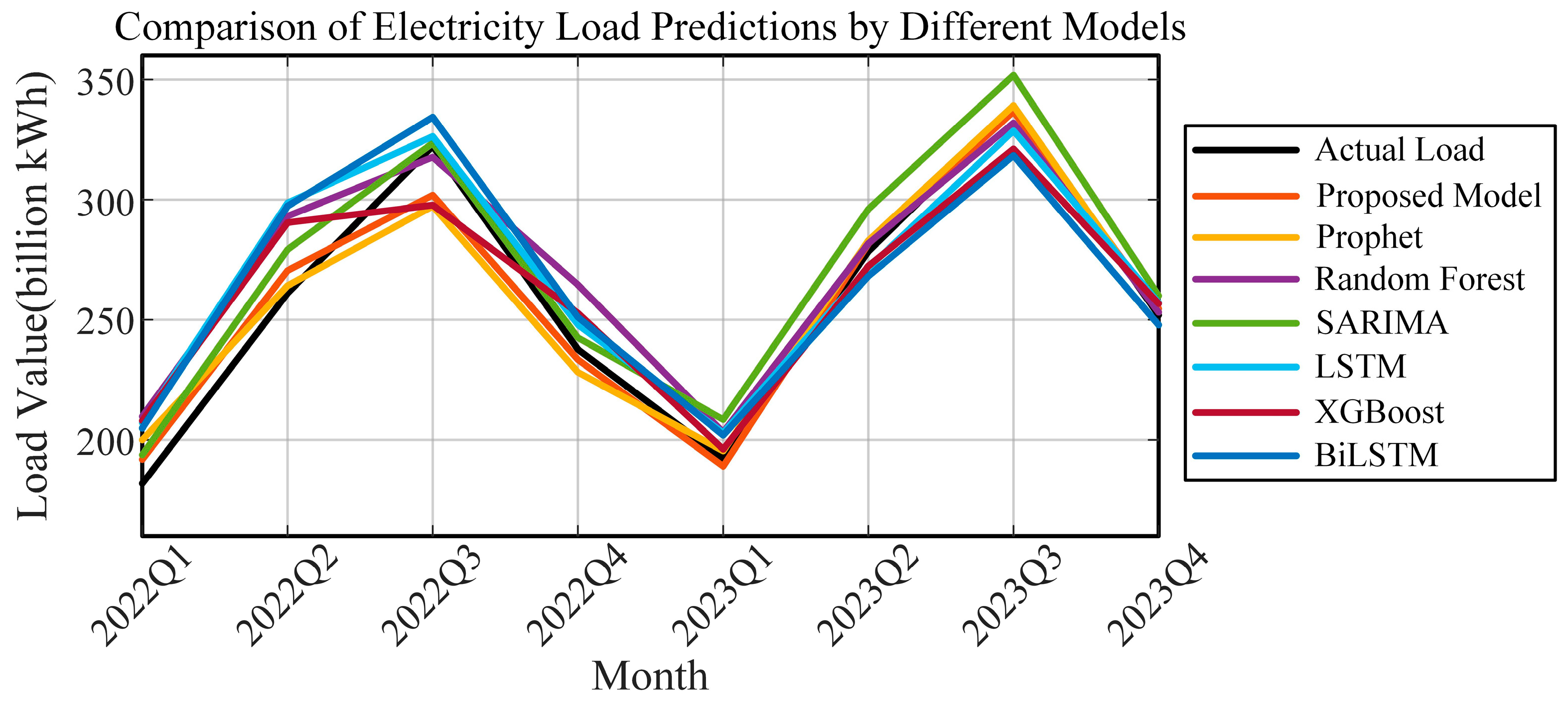
The quarterly forecast results are compared with those of other typical models, as shown in Figure 12 and

Table 6. Quarterly forecasting results for Case I using different models.

Models	MAPE (%)	MAE (100 Million kWh)	RMSE (100 Million kWh)	R2 (%)	Bias (100 Million kWh)
Proposed Model	2.66	6.74	9.02	96.97	−0.425
Prophet	3.40	8.29	11.68	94.93	−0.325
RF	6.18	14.09	18.44	87.35	11.51
SARIMA	4.78	11.57	12.97	93.74	11.58
LSTM	5.83	13.62	17.48	88.63	9.67
XGBoost	6.33	15.82	18.45	87.33	4.03
BiLSTM	6.51	16.02	18.57	87.17	7.62

.

It can be observed that the proposed model outperforms other models in quarterly forecasting, while models based on large datasets, such as LSTM and BiLSTM, show noticeably poorer performance. Overall, the proposed model demonstrates excellent performance in quarterly forecasting.

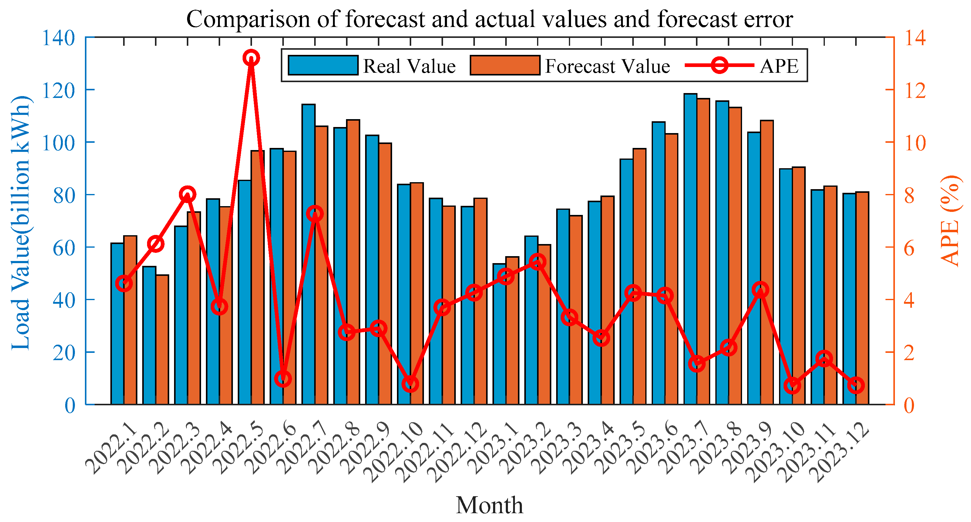
Similarly, for the monthly forecasting scenario, the methodology follows the same approach as the quarterly forecasts. The results for a total of 24 months, spanning from 2022 to 2023, are used for validation and analysis. The forecast results are presented in

Table 7. Forecast results of electricity consumption by month in 2022 and 2023 (unit/billion kWh).

Periods	2022.1	2022.2	2022.3	2022.4	2022.5	2022.6	2022.7	2022.8
Real Value	61.40	52.55	67.89	78.28	85.40	97.47	114.34	105.47
Forecast Value	64.22	49.33	73.33	75.36	96.68	96.51	106.03	108.37
APE	4.61%	6.12%	8.01%	3.73%	13.21%	0.98%	7.27%	2.75%
Periods	2022.9	2022.10	2022.11	2022.12	2023.1	2023.2	2023.3	2023.4
Real Value	102.54	83.81	78.51	75.38	53.58	64.13	74.43	77.37
Forecast Value	99.57	84.46	75.60	78.59	56.19	60.82	71.96	79.33
APE	2.90%	0.78%	3.70%	4.26%	4.88%	5.44%	3.32%	2.53%
Periods	2023.5	2023.6	2023.7	2023.8	2023.9	2023.10	2023.11	2023.12
Real Value	93.50	107.61	118.38	115.62	103.66	89.80	81.78	80.35
Forecast Value	97.47	103.15	116.54	113.10	108.19	90.44	83.21	80.94
APE	4.25%	4.15%	1.55%	2.17%	4.37%	0.72%	1.75%	0.73%

and Figure 13.

For monthly forecasts, the forecast error tends to be larger due to the smaller total electricity consumption compared to quarterly and annual forecasts, even when the deviation value is the same. However, the majority of the monthly forecast errors remain within 5%, and the overall MAPE value for the 24-month period is 3.92%. This indicates a relatively small overall error, highlighting the model’s strong forecasting performance.

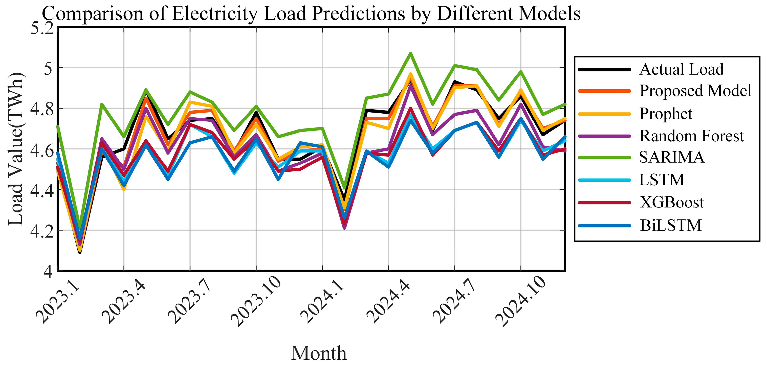
Similarly, the monthly forecasting model is also compared with other models, and the comparison results are shown in Figure 14 and

Table 8. Monthly forecasting results for Case I using different models.

Models	MAPE (%)	MAE (Billion kWh)	RMSE (Billion kWh)	R2 (%)	Bias (Billion kWh)
Proposed Model	3.91	3.25	4.01	95.42	0.256
Prophet	4.80	3.84	4.94	93.06	−0.068
RF	7.59	5.95	7.52	83.91	3.764
SARIMA	5.21	4.13	5.56	91.22	3.860
LSTM	6.14	5.05	6.20	89.05	1.762
XGBoost	6.13	5.08	7.06	85.84	1.398
BiLSTM	7.01	5.63	7.89	82.31	2.818

.

As seen from the table, similar to the quarterly forecast, the proposed model achieves the best performance in monthly forecasting as well, consistently delivering relatively better results across various metrics, and demonstrates excellent performance in monthly predictions.

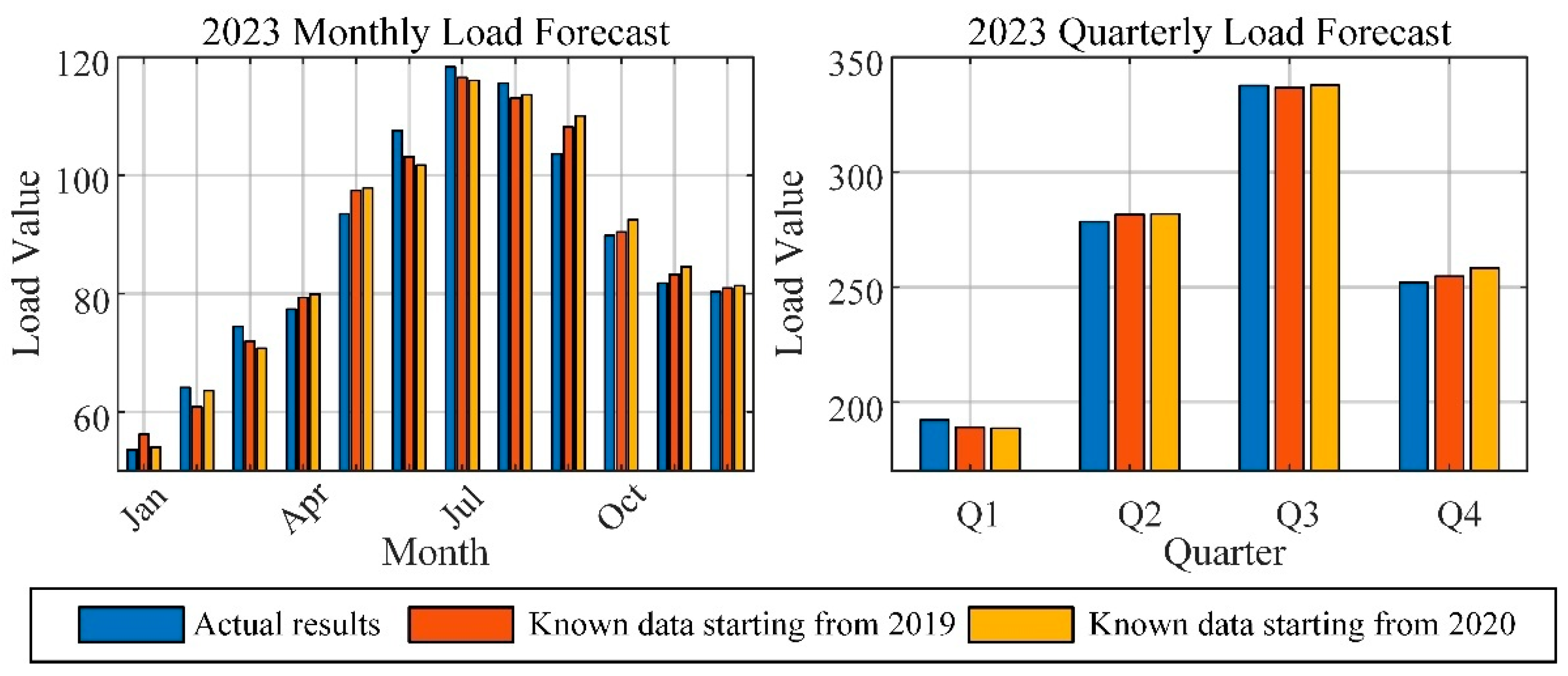
Based on the above analysis, we can also briefly discuss the impact of the training data size on the forecasting results. In the analysis above, when forecasting electricity consumption for a given period, all the data prior to that period are used as known data and added to the training set. For example, when forecasting a specific period in 2023, the available training data include an entire additional year (2022) compared to the same period in 2022. Therefore, overall, the prediction performance for 2023 is better than that for 2022. When analyzing 2023, we can consider using training sets of different lengths to analyze and assess the impact of the training set length on the forecasting results. The analysis is conducted using data from 2019 to 2022 and from 2020 to 2022 as training sets to forecast the electricity consumption in 2023. The analysis results are shown in

Table 9. Forecast results for 2023 with different training set lengths.

Existing Data	Annual Forecast (APE)	Quarterly Forecast (MAPE)	Monthly Forecast (MAPE)
From 2019	0.39%	1.02%	2.99%
From 2020	0.53%	1.41%	3.13%

and Figure 15.

It can be seen that as the training set contains more data, the model’s performance improves. Overall, the 2023 data align better with the historical variation patterns compared to 2022. Therefore, when trained with three years of data, the forecasting performance for 2023 is better than that for 2022.

As demonstrated by the above analysis, the proposed method is capable of simultaneously predicting electricity consumption data across monthly, quarterly, and annual timescales. The overall prediction accuracy is highest for annual forecasts, followed by quarterly and then monthly forecasts. In this dataset, the overall accuracy of the annual forecasts is within 2%; the MAPE for quarterly forecasts is below 3%; and the MAPE for monthly forecasts is below 4%. The method demonstrates high accuracy.

5.3. Case Ⅱ

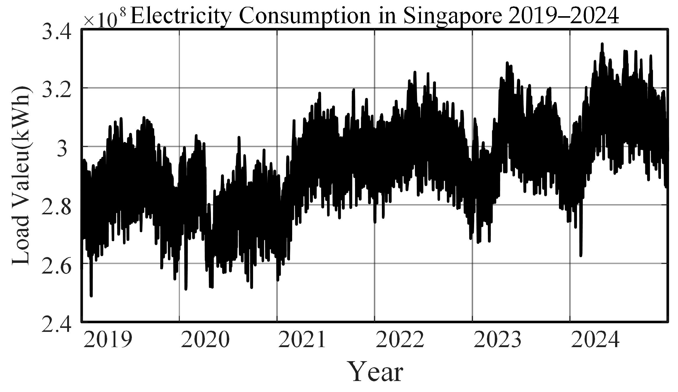
To validate the generalizability of the proposed model, predictions were also made on other datasets. In this case, the electricity demand data for Singapore from 2019 to 2024 were selected for study, with the corresponding data provided by the Energy Market Company [46]. The holiday data for Singapore used in the analysis were sourced from the holidays library (version 0.37) in Python. The variation in Singapore’s daily load during the analyzed period is shown in Figure 16.

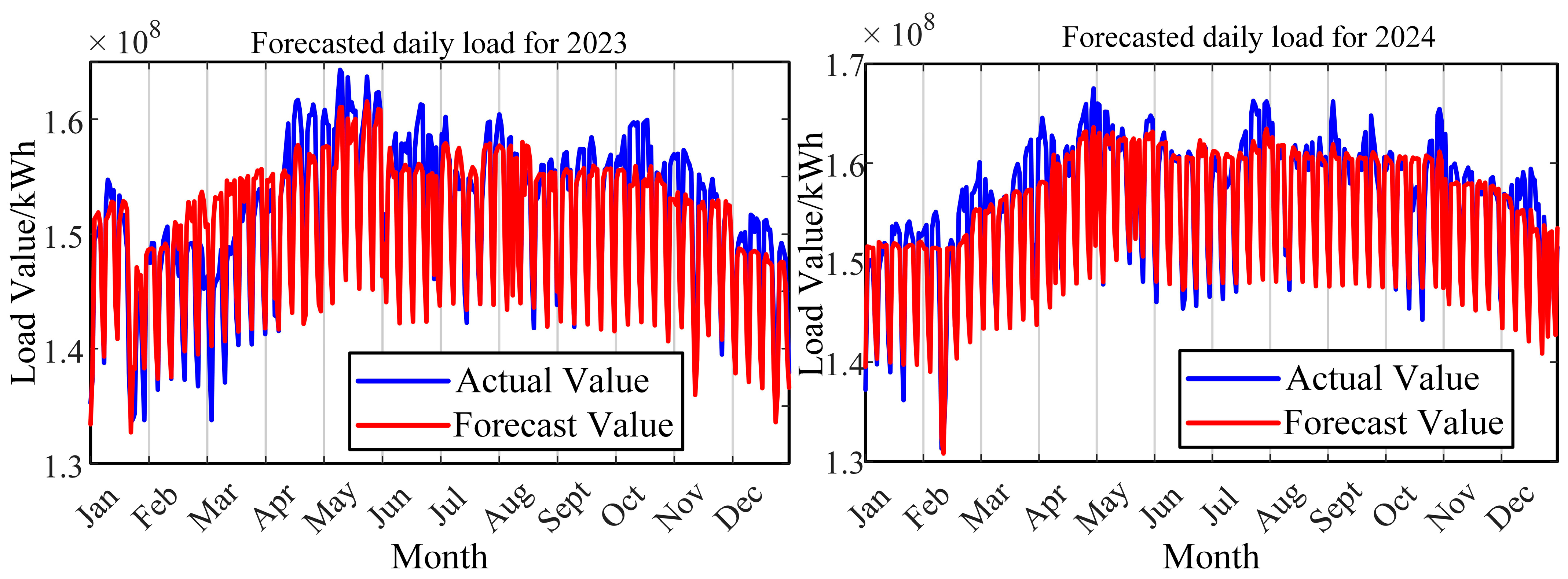
The analysis method is the same as in Case 1. In predicting Singapore’s annual electricity consumption, the values for 2023 and 2024 are 55.22 TWh and 56.98 TWh, respectively. The prediction results for 2023 and 2024 using the proposed method are shown in Figure 17, and the performance of different methods in annual forecasting is presented in

Table 10. Comparison of predicted values and actual values from different algorithms.

Model	2023			2024			Average Runtime
	Forecast Value (TWh)	APE (%)	AE (TWh)	Forecast Value (TWh)	APE (%)	AE (TWh)
Prophet–RF	54.94	0.51	0.28	56.69	0.50	0.29	2.41 s
Prophet	53.99	2.23	1.23	56.29	1.20	0.69	1.65 s
Random Forest	55.00	0.40	0.22	55.83	2.01	1.15	0.67 s
Cubic Exponential Smoothing	53.70	2.75	1.52	55.62	2.45	1.36	0.44 s
SARIMA	56.56	2.44	1.34	58.12	2.01	1.14	0.63 s
Gray Forecast	57.36	3.87	2.14	57.08	0.18	0.10	0.16 s
LSTM	54.14	1.96	1.08	54.97	3.53	2.01	9.26 s
XGBoost	54.77	0.81	0.45	55.30	2.94	1.68	0.71 s
BiLSTM	54.01	2.18	1.21	54.79	3.84	2.19	14.87 s

.

From the above information, it can be seen that, overall, the proposed algorithm achieves an average quarterly error of within 1% for both 2023 and 2024, and can generate results in a relatively short time, demonstrating good performance. Additionally, owing to the more consistent nature of the Singaporean data compared with that of southern Chinese cities, all algorithms in Case 2 exhibit better accuracy than those in Case 1.

For quarterly forecasting, the prediction results are shown in Figure 18 and

Table 11. Quarterly forecasting results for Case II using different models.

Models	MAPE (%)	MAE (TWh)	RMSE (TWh)	R2 (%)	Bias (TWh)
Proposed Model	0.53	0.075	0.101	94.13	−0.025
Prophet	1.2	0.174	0.269	58.21	−0.076
RF	1.62	0.228	0.250	63.70	−0.188
SARIMA	2.22	0.309	0.334	35.56	0.309
LSTM	2.76	0.391	0.436	−10.13	−0.351
XGBoost	2.25	0.316	0.346	30.90	−0.251
BiLSTM	2.75	0.390	0.455	−19.87	−0.353

.

From the above analysis, it can be seen that in quarterly prediction, the proposed algorithm also achieves the best performance, with MAPE values within 1% on this dataset, demonstrating exceptional performance.

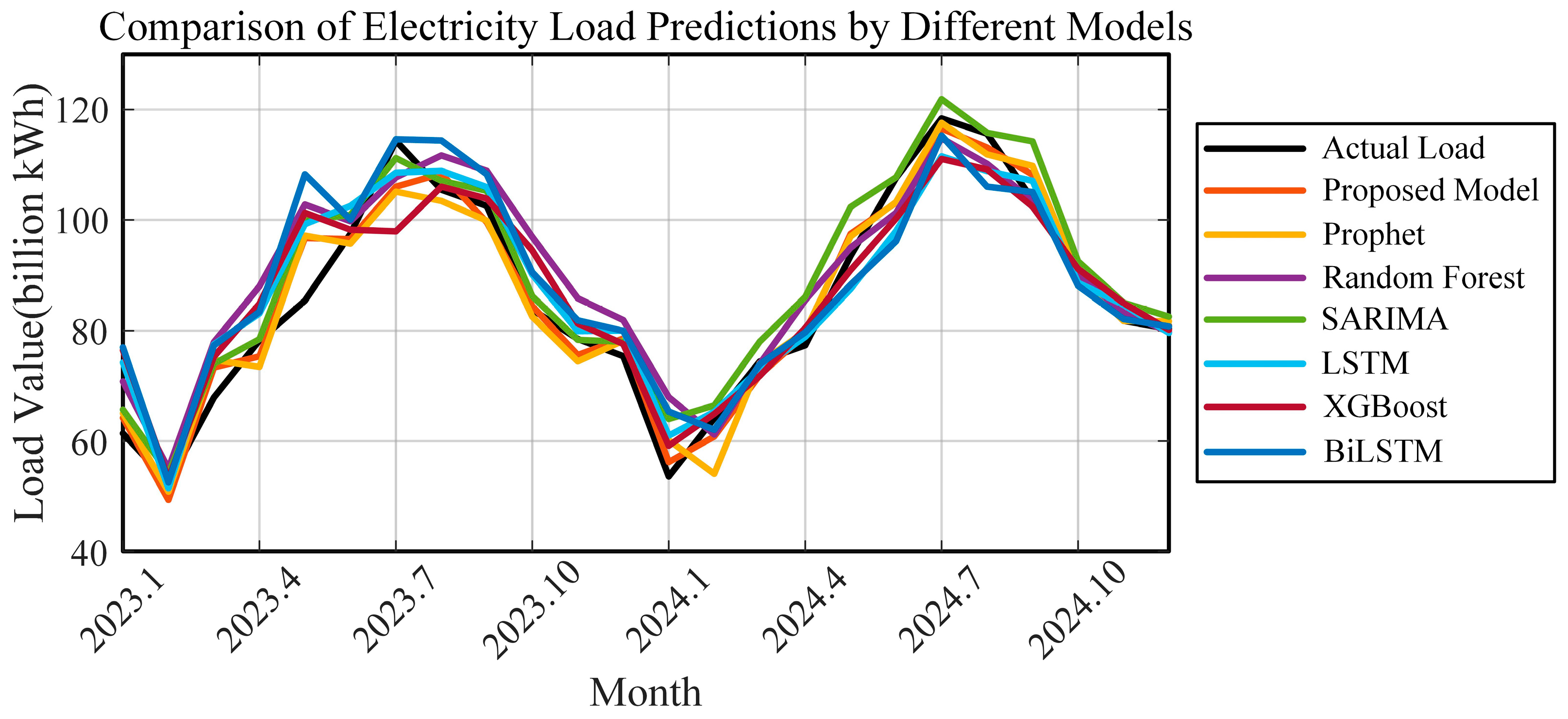
For monthly prediction, the results are shown in Figure 19 and

Table 12. Monthly forecasting results for Case II using different models.

Models	MAPE (%)	MAE (TWh)	RMSE (TWh)	R2 (%)	Bias (TWh)
Proposed Model	0.59	0.028	0.033	96.94	−0.005
Prophet	1.00	0.047	0.065	88.26	−0.013
RF	1.67	0.079	0.098	73.33	−0.065
SARIMA	2.20	0.102	0.114	63.36	0.102
LSTM	2.58	0.122	0.142	43.36	−0.106
XGBoost	2.46	0.116	0.134	49.50	−0.105
BiLSTM	2.82	0.133	0.150	36.50	−0.112

.

Based on the above analysis, the proposed model also achieves the best performance in monthly prediction, with the forecast MAPE value staying within 1% on this dataset.

In summary, it can be concluded that the proposed model achieves the best predictive performance for the Singapore electricity dataset, whether for annual, quarterly, or monthly forecasts. Given that Singapore’s electricity data exhibit relatively low volatility and stable overall characteristics, the model delivers excellent results, with the average MAPE for monthly, quarterly, and annual forecasts remaining below 1%. Moreover, the model can complete calculations within 3 s without the need for GPU acceleration, demonstrating low resource consumption and strong operability, making it highly applicable and valuable for broader adoption.

6. Conclusions

This paper proposes a multi-scale forecasting approach that integrates the Prophet algorithm with the Random Forest (RF) model for medium- to long-term electricity load prediction. Compared to using either Prophet or RF alone, the combined approach achieves significantly improved forecasting accuracy. It also outperforms several conventional algorithms in predictive effectiveness. When applied to electricity consumption data from cities in southern China, the model achieves forecasting errors within 2%, 3%, and 4% for annual, quarterly, and monthly timescales, respectively. For Singapore’s electricity demand, the prediction errors at all three temporal scales remain below 1%, demonstrating excellent forecasting capability. In terms of computational cost, while the runtime is higher than that of traditional models such as SARIMA, XGBoost, and RF, it is considerably lower than that of deep learning models like LSTM. Overall, the proposed model offers high predictive accuracy, strong applicability, and robust generalizability.

However, the model has certain limitations. If large portions of historical data are missing, or if future electricity usage patterns differ significantly from past trends due to unforeseen factors, the model—relying on historical data—may result in substantial errors. Future work could address this by incorporating additional external variables (e.g., weather, policy changes, and unexpected events) and developing hybrid or adaptive frameworks to enhance the model’s responsiveness and robustness under uncertainty.

References

1. Yan, X.; Xin, B.; Cheng, C.; Han, Z. Unpacking energy consumption in China’s urbanization: Industry development, population growth, and spatial expansion. Res. Int. Bus. Financ. 2024, 70, 102342. [Google Scholar] [CrossRef]
2. Lin, B.; Zhu, J. Chinese electricity demand and electricity consumption efficiency: Do the structural changes matter? Appl. Energy 2020, 262, 114505. [Google Scholar] [CrossRef]
3. Hahn, H.; Meyer-Nieberg, S.; Pickl, S. Electric load forecasting methods: Tools for decision making. Eur. J. Oper. Res. 2009, 199, 902–907. [Google Scholar] [CrossRef]
4. Hong, T.; Pinson, P.; Fan, S.; Zareipour, H.; Troccoli, A.; Hyndman, R.J. Probabilistic energy forecasting: Global Energy Forecasting Competition 2014 and beyond. Int. J. Forecast. 2016, 32, 896–913. [Google Scholar] [CrossRef]
5. Hong, T.; Pinson, P.; Wang, Y.; Weron, R.; Yang, D.Z.; Zareipour, H. Energy Forecasting: A Review and Outlook. IEEE Open Access J. Power Energy 2020, 7, 376–388. [Google Scholar] [CrossRef]
6. Dudek, G. Pattern-based local linear regression models for short-term load forecasting. Electr. Power Syst. Res. 2016, 130, 139–147. [Google Scholar] [CrossRef]
7. Di, J.; Qi, B. Short-term Power Load Forecasting based on Big Data. Int. Core J. Eng. 2021, 7, 266–270. [Google Scholar] [CrossRef]
8. Morita, H.; Zhang, D.P.; Tamura, Y. Long-term load forecasting using grey system theory. Electr. Eng. Jpn. 1995, 115, 11–20. [Google Scholar] [CrossRef]
9. Mirasgedis, S.; Sarafidis, Y.; Georgopoulou, E.; Lalas, D.P.; Moschovits, M.; Karagiannis, F.; Papakonstantinou, D. Models for mid-term electricity demand forecasting incorporating weather influences. Energy 2006, 31, 208–227. [Google Scholar] [CrossRef]
10. Wu, F.; Cattani, C.; Song, W.; Zio, E. Fractional ARIMA with an improved cuckoo search optimization for the efficient Short-term power load forecasting. Alex. Eng. J. 2020, 59, 3111–3118. [Google Scholar] [CrossRef]
11. Munkhammar, J.; van der Meer, D.; Widén, J. Very short term load forecasting of residential electricity consumption using the Markov-chain mixture distribution (MCM) model. Appl. Energy 2021, 282, 116180. [Google Scholar] [CrossRef]
12. Alhendi, A.; Al-Sumaiti, A.S.; Marzband, M.; Kumar, R.; Diab, A.A.Z. Short-term load and price forecasting using artificial neural network with enhanced Markov chain for ISO New England. Energy Rep. 2023, 9, 4799–4815. [Google Scholar] [CrossRef]
13. Aswanuwath, L.; Pannakkong, W.; Buddhakulsomsiri, J.; Karnjana, J.; Huynh, V.N. A Hybrid Model of VMD-EMD-FFT, Similar Days Selection Method, Stepwise Regression, and Artificial Neural Network for Daily Electricity Peak Load Forecasting. Energies 2023, 16, 1860. [Google Scholar] [CrossRef]
14. Guan, C.; Luh, P.B.; Michel, L.D.; Chi, Z. Hybrid Kalman filters for very short-term load forecasting and prediction interval estimation. IEEE Trans. Power Syst. 2013, 28, 3806–3817. [Google Scholar] [CrossRef]
15. Zheng, Z.; Chen, H.; Luo, X. A Kalman filter-based bottom-up approach for household short-term load forecast. Appl. Energy 2019, 250, 882–894. [Google Scholar] [CrossRef]
16. Hou, H.; Liu, C.; Wang, Q.; Wu, X.; Tang, J.; Shi, Y.; Xie, C. Review of load forecasting based on artificial intelligence methodologies, models, and challenges. Electr. Power Syst. Res. 2022, 210, 108067. [Google Scholar] [CrossRef]
17. Aouad, M.; Hajj, H.; Shaban, K.; Jabr, R.A.; El-Hajj, W. A CNN-Sequence-to-Sequence network with attention for residential short-term load forecasting. Electr. Power Syst. Res. 2022, 211, 108152. [Google Scholar] [CrossRef]
18. Wang, W.; Chen, Y.; Xiao, C.; Yang, Y.; Yao, J. Design of short-term load forecasting method considering user behavior. Electr. Power Syst. Res. 2024, 234, 110529. [Google Scholar] [CrossRef]
19. Eskandari, H.; Imani, M.; Moghaddam, M.P. Convolutional and recurrent neural network based model for short-term load forecasting. Electr. Power Syst. Res. 2021, 195, 107173. [Google Scholar] [CrossRef]
20. Casolaro, A.; Capone, V.; Iannuzzo, G.; Camastra, F. Deep Learning for Time Series Forecasting: Advances and Open Problems. Information 2023, 14, 598. [Google Scholar] [CrossRef]
21. Chen, Z.; Ma, M.; Li, T.; Wang, H.; Li, C. Long sequence time-series forecasting with deep learning: A survey. Inf. Fusion 2023, 97, 101819. [Google Scholar] [CrossRef]
22. Shi, H.; Xu, M.; Li, R. Deep learning for household load forecasting—A novel pooling deep RNN. IEEE Trans. Smart Grid 2017, 9, 5271–5280. [Google Scholar] [CrossRef]
23. Hong, Y.; Zhou, Y.; Li, Q.; Xu, W.; Zheng, X. A deep learning method for short-term residential load forecasting in smart grid. IEEE Access 2020, 8, 55785–55797. [Google Scholar] [CrossRef]
24. Kalhori, M.R.N.; Emami, I.T.; Fallahi, F.; Tabarzadi, M. A data-driven knowledge-based system with reasoning under uncertain evidence for regional long-term hourly load forecasting. Appl. Energy 2022, 314, 118975. [Google Scholar] [CrossRef]
25. Muñoz, M.C.; Peñalba, M.A.; González, A.E.S. Analysis of aggregated load consumption forecasting in short, medium and long term horizons using dynamic mode decomposition. Energy Rep. 2024, 12, 1000–1013. [Google Scholar] [CrossRef]
26. Pełka, P. Analysis and forecasting of monthly electricity demand time series using pattern-based statistical methods. Energies 2023, 16, 827. [Google Scholar] [CrossRef]
27. Kanté, M.; Li, Y.; Deng, S. Scenarios analysis on electric power planning based on multi-scale forecast: A case study of Taoussa, Mali from 2020 to 2035. Energies 2021, 14, 8515. [Google Scholar] [CrossRef]
28. Li, J.; Luo, Y.; Wei, S. Long-term electricity consumption forecasting method based on system dynamics under the carbon-neutral target. Energy 2022, 244, 122572. [Google Scholar] [CrossRef]
29. Zhang, S.; Liu, J.; Wang, J. High-Resolution Load Forecasting on Multiple Time Scales Using Long Short-Term Memory and Support Vector Machine. Energies 2023, 16, 1806. [Google Scholar] [CrossRef]
30. Jiang, Y.; Li, Y.; Chen, Y. Interpretable short-term load forecasting via multi-scale temporal decomposition. Electr. Power Syst. Res. 2024, 235, 110781. [Google Scholar] [CrossRef]
31. Wan, A.; Gong, Z.; Wei, C.; AL-Bukhaiti, K.; Ji, Y. Multistep Forecasting Method for Offshore Wind Turbine Power Based on Multi-Timescale Input and Improved Transformer. J. Mar. Sci. Eng. 2024, 12, 925. [Google Scholar] [CrossRef]
32. Ma, D.; Wu, R.; Li, Z.; Cen, K.; Gao, J.; Zhang, Z. A new method to forecast multi-time scale load of natural gas based on augmentation data-machine learning model. Chin. J. Chem. Eng. 2022, 48, 166–175. [Google Scholar] [CrossRef]
33. Zheng, K.; Li, P.; Zhou, S.; Zhang, W.; Li, S.; Zeng, L. A multi-scale electricity consumption prediction algorithm based on time-frequency variational autoencoder. IEEE Access 2021, 9, 90937–90946. [Google Scholar] [CrossRef]
34. Xu, X.; Niu, D.; Fu, M.; Xia, H.; Wu, H. A multi time scale wind power forecasting model of a chaotic echo state network based on a hybrid algorithm of particle swarm optimization and tabu search. Energies 2015, 8, 12388–12408. [Google Scholar] [CrossRef]
35. Sun, Y.; Guo, X.; Huangfu, X.; Ma, J.; Fan, J.; Zhang, H.; Ren, Z. Multi-time scales load forecasting based on hybrid neural network. Adv. Technol. Electr. Eng. Energy 2023, 42, 95–104. [Google Scholar] [CrossRef]
36. Zhu, S.; Wang, J.; Zhao, W.; Wang, J. A seasonal hybrid procedure for electricity demand forecasting in China. Appl. Energy 2011, 88, 3807–3815. [Google Scholar] [CrossRef]
37. Rouhani, A.; Mashhadi, H.R.; Feizi, M. Estimating the Short-term Price Elasticity of Residential Electricity Demand in Iran. Int. Trans. Electr. Energy Syst. 2022, 2022, 4233407. [Google Scholar] [CrossRef]
38. Liu, Y.; Zhao, J.; Liu, J.; Chen, Y.; Ouyang, H. Regional midterm electricity demand forecasting based on economic, weather, holiday, and events factors. IEEJ Trans. Electr. Electron. Eng. 2020, 15, 225–234. [Google Scholar] [CrossRef]
39. Song, K.; Park, J.; Park, R. Short Term Load Forecasting Algorithm for Lunar New Year’s Day. J. Electr. Eng. Technol. 2018, 13, 591–598. [Google Scholar] [CrossRef]
40. Hussain, A.; Giangrande, P.; Franchini, G.; Fenili, L.; Messi, S. Analyzing the Effect of Error Estimation on Random Missing Data Patterns in Mid-Term Electrical Forecasting. Electronics 2025, 14, 2079–9292. [Google Scholar] [CrossRef]
41. Wang, X.; Yao, Z.; Papaefthymiou, M. A real-time electrical load forecasting and unsupervised anomaly detection framework. Appl. Energy 2023, 330, 120279. [Google Scholar] [CrossRef]
42. Chakhchoukh, Y.; Panciatici, P.; Mili, L. Electric load forecasting based on statistical robust methods. IEEE Trans. Power Syst. 2010, 26, 982–991. [Google Scholar] [CrossRef]
43. Breiman, L. Random forests. Mach. Learn. 2001, 45, 5–32. [Google Scholar] [CrossRef]
44. EI-Azab, H.A.I.; Swief, R.A.; EI-Amary, N.H.; Temraz, H.K. Seasonal forecasting of the hourly electricity demand applying machine and deep learning algorithms impact analysis of different factors. Sci. Rep. 2025, 15, 9252. [Google Scholar] [CrossRef] [PubMed]
45. Son, N.; Shin, Y. Short- and Medium-Term Electricity Consumption Forecasting Using Prophet and GRU. Sustainability 2023, 15, 15860. [Google Scholar] [CrossRef]
46. Energy Market Company. NEMS Market Prices. Available online: https://www.nems.emcsg.com/nems-prices (accessed on 17 July 2025).
Figure 1. Predictive modeling flowchart.
Energies 18 04378 g001
Figure 2. Schematic diagram of Spring Festival correction.
Energies 18 04378 g002
Figure 3. Random Forest algorithm.
Energies 18 04378 g003
Figure 4. Input–output structure of the prediction model.
Energies 18 04378 g004
Figure 5. Improvement of the 3σ guideline.
Energies 18 04378 g005
Figure 6. Load correction results.
Energies 18 04378 g006
Figure 7. The output of the Prophet model with different influencing factors. Line 1: Actual electricity consumption in 2023. Line 2: Prophet model prediction for 2023 considering annual seasonality, weekly seasonality, and holiday effects (baseline model). Line 3: Prophet model prediction excluding annual seasonality. Line 4: Prophet model prediction excluding weekly seasonality. Line 5: Prophet model prediction excluding holiday effects. Line 6: Prophet model prediction including monthly seasonality in addition to the baseline. Line 7: Prophet model prediction including quarterly seasonality in addition to the baseline. Line 8: Prophet model prediction including both monthly and quarterly seasonality in addition to the baseline.
Energies 18 04378 g007
Figure 8. MSE for different hyperparameters.
Energies 18 04378 g008
Figure 9. The OOB error during the training process.
Energies 18 04378 g009
Figure 10. Forecasted daily load for 2022 and 2023.
Energies 18 04378 g010
Figure 11. Quarterly forecasts for 2022 and 2023.
Energies 18 04378 g011
Figure 12. Quarterly forecasting results for Case I using different models.
Energies 18 04378 g012
Figure 13. Monthly forecasts for 2022 and 2023.
Energies 18 04378 g013
Figure 14. Monthly forecasting results for Case I using different models.
Energies 18 04378 g014
Figure 15. Forecast results for 2023 with different training set lengths.
Energies 18 04378 g015
Figure 16. Electricity consumption in Singapore in 2019–2024.
Energies 18 04378 g016
Figure 17. Forecasted daily load for 2023 and 2024.
Energies 18 04378 g017
Figure 18. Quarterly forecasting results for Case II using different models.
Energies 18 04378 g018
Figure 19. Monthly forecasting results for Case II using different models.
Energies 18 04378 g019