Non-Parametric Loop-Shaping Algorithm for High-Order Servo Systems Based on Preset Frequency Domain Specifications

Abstract

Loop shaping the controller for high-order systems, especially in the presence of flexible transmission components such as elastic shafts, gearboxes, and belts commonly found in servo systems, poses significant challenges. Therefore, developing a non-parametric, versatile tuning algorithm that adapts to multi-order systems is essential for general control applications. This article first obtains the frequency characteristics of plants through a frequency sweep. Then, based on preset frequency domain specifications, the boundaries representing disturbance rejection and stability constraints are defined in the complex plane with explicit mathematical and graphical expressions. Subsequently, a system of equations is developed based on the tangency between the open-loop curve of the system and the boundaries in the complex plane. On this basis, a versatile tuning algorithm is designed to calculate parameters of a PI controller cascaded with a low-pass filter that ensures the system meets the preset constraints. The proposed approach does not rely on parametric modeling, and the zeros and poles of the controller can be flexibly placed. Experimental validation is carried out on mechanical platforms.

1. Introduction

In the fields of industrial manufacturing and motion control, the plant’s frequency characteristics are often marked by complexity and diversity, for example, the prototype target table positioning system adopted in [1], the electric injection molding machine used in [2], the hybridized city bus tested in [3], and the ABB IRB 1400 type robot utilized in [4]. These plants exhibit multiple resonant modes across different frequency ranges, each characterized by distinct magnitudes and phases. When resonant modes appear in the low-frequency region, the closed-loop bandwidth of the system can be severely restricted. This results in increased system complexity and diversity. In the context of linear control theory, when designing controller parameters for the systems corresponding to the controlled plants in [1,2,3,4], traditional tuning strategies based on plant modeling and parameter identification may become ineffective. This is because the diversity and complexity of the frequency characteristics exhibited by general controlled plants often lead to low model accuracy and poor identification reliability. Therefore, the development of automatic tuning algorithms for controller parameter computation is essential.

Some controller tuning strategies focus on time-domain metrics (such as overshoot, rise and settling time, etc.) derived from experimental results, represented by the Ziegler–Nichols (ZN) method [5,6,7]. The ZN method is not commonly used in practice as it is time-consuming, labor-intensive, and requires close attention from the operator. To this end, Rad et al. [8] designed an iterative PI parameter-tuning algorithm based on the Newton–Raphson method. While the designed algorithm is computationally efficient, its convergence and robustness exhibit some degree of uncertainty. In Ref. [9], a genetic algorithm was used, with overshoot and the integral of weighted time absolute error as cost functions, to achieve the optimized design of the PID controller. Cheng et al. [10] combined gradient optimization with fuzzy step-sizing techniques, using time-domain metrics such as overshoot and tracking error as predefined objective functions to design an optimal controller. Similarly, Tursini et al. [11] proposed a real-time, model-free tuning method for the PI speed controller based on the integral error (IE) between the actual and ideal overshoot. These methods face challenges in converting time-domain metrics into intuitive constraints on the open-loop transfer function, often relying on iterative or trial-and-error tuning procedures. As a result, they may lead to issues such as high computational burden, system instability, and poor convergence.

Model-based tuning methods are the most common in the field of linear control, among which the zero-pole cancellation (ZPC) method optimizes dynamic performance by canceling the plant dominant pole with the controller zero [12,13,14]. Yang et al. [15] modeled both the current- and speed-loop of the servo system as simple first-order models, and based on this, performed offline identification of electrical and mechanical parameters to achieve ZPC. Erturk et al. [16] proposed a voltage injection method to estimate a spatial inductance map, and the inductance parameter was then used to tune the PI controller of the current loop based on ZPC. Model predictive control (MPC) includes two main strategies: model predictive torque control (MPTC) and model predictive current control (MPCC) [17]. MPTC requires the joint regulation of torque and flux linkage, making it necessary to design a cost function with suitable weighting factors to balance these variables [18]. In contrast, MPCC focuses solely on current control. Since its cost function deals with variables of the same dimension, MPCC eliminates the need for weighting factors, resulting in a simpler implementation than MPTC [19,20]. For the first-order current-loop system, Shang et al. [21] introduced the normalized gain as the sole variable in the PI controller and achieved ZPC in the form of parameter correction. In second-order speed servo systems, a strategy known as ‘double ratio’ is widely used for tuning PI controllers [22]. Similar to ZPC, this tuning method relies on model parameters, namely the motor and load inertia values, and the resulting PI controller has only a single adjustable variable. Although both ZPC and the double ratio method offer strong control performance for the system, they rely on high-precision parameter identification or self-correction processes. Moreover, the designed controller features a single tuning variable, limiting its flexibility and making it challenging to adapt to multiple resonant modes (high-order) systems.

Apart from ZPC, another category of strategies emphasizes the frequency-domain specifications of the system. Refs. [23,24] employed gain and phase margins for PID controller tuning. In [25], a fractional-order PID with multiple adjustable variables is employed, with its parameters sequentially adjusted based on five frequency-domain specifications. Tuning using multiple frequency-domain specifications in [23,24,25] can increase the number of adjustable parameters in the controller. The quantitative feedback theory (QFT) [26,27] enables the visualization of preset frequency-domain specifications in the Nichols plot, thereby facilitating the design of the controller. However, the resulting controllers may lack practicality due to their potentially high order, and both the controller structure and parameter design require manual intervention. In [28,29,30,31], a strategy called ‘circle-condition’ is adopted to quantify and visualize gain and phase margins as graphical elements in the Nyquist plot. Unlike QFT, this approach can facilitate the analytical computation of loop shaping, which reduces the need for manual operation. ‘Circle-condition’ treats gain and phase margins as a single adjustable variable, making it difficult to impose performance constraints on high-order systems. Building on the ‘circle-condition’, this paper treats gain and phase margins as two independent variables, quantifies and visualizes multiple frequency-domain specifications in the complex plane, and proposes a non-parametric, versatile tuning algorithm that adapts to multi-order systems, reducing the need for manual intervention.

Addressing the limitations of traditional tuning methods, which are constrained by specific models and lack general applicability, the proposed non-parametric tuning algorithm presents the following features and contributions:

• The algorithm is applicable to plants with multiple resonant points (multi-order), ensuring a certain degree of versatility. The plant data can be measured or pre-recorded;
• By presetting the frequency-domain specifications, the algorithm ensures that the system exhibits desired dynamic characteristics within a specific frequency range, such as low overshoot, fast response time, and excellent disturbance rejection performance;
• Since the mathematical and graphical representations of the constraint boundary in the complex plane are well-defined and visible, the algorithmic design process based on the boundary is highly transparent;
• The tuning results of the algorithm exhibit consistency for identical types of plants, as reflected in similar time-domain metrics, such as overshoot and speed drop.

This paper is organized as follows. In Section 2, the system structure and frequency sweep strategy employed in this paper are introduced. Based on preset frequency-domain specifications, the stability and disturbance rejection constraints are sequentially constructed, ultimately forming a constraint boundary that covers the entire frequency range in a linear coordinate system. In Section 3, a search algorithm is proposed to obtain a set of controller parameters that ensure both excellent system stability and dynamic performance. Furthermore, a validation algorithm is introduced to address the issue of local failure. Finally, the experiments and conclusions are presented in Section 4 and Section 5, respectively.

2. Frequency Domain Modeling and Constraint Boundaries

In this section, the frequency characteristics of the plant are first obtained through a frequency sweep. To achieve the desired dynamic response, the closed-loop magnitude constraint for stability and the sensitivity constraint for disturbance rejection are established based on preset frequency-domain specifications, including gain and phase margins. These constraints are quantized and visualized in the complex plane to define the constraint boundaries across the entire frequency range.

2.1. System Structure and Frequency Sweep

The unit negative feedback closed-loop system employed in this paper is shown in Figure 1. A low-pass filter is cascaded with a PI controller to reduce sensor noise and enhance the performance of the closed-loop system [32]. Chirp is used as the injected sweep signal, with the frequency set Ω defined by the initial, step, and final frequencies ω_start, ω_step, and ω_end. The collected signals S_in(jω) and S_out(jω) are then processed to obtain the frequency characteristics H(jω) of the plant: H(jω) = X_H(ω) + jY_H(ω), X_H(ω) = |H(jω)|·cos(∠H(jω)), Y_H(ω) = |H(jω)|·sin(∠H(jω)), where |H(jω)| and ∠H(jω) are the magnitude and phase of H(jω), respectively.

As shown in Figure 1, the closed-loop transfer function G_cl(jω) can be derived as follows:

$$G_{cl}(j\omega )={\displaystyle \frac{feedback\left(j\omega \right)}{reference\left(j\omega \right)}}={\displaystyle \frac{L\left(j\omega \right)}{1+L\left(j\omega \right)}}={\displaystyle \frac{K_p(K_i+j\omega )G_{f}H}{K_p(K_i+j\omega )G_{f}H+j\omega }}$$

(1)

where L(jω) represents the open-loop transfer function of system, with L(jω) = X_L(ω) + jY_L(ω), and G_f(jω) denotes the transfer function of the filter.

2.2. Stability Constraint Boundary

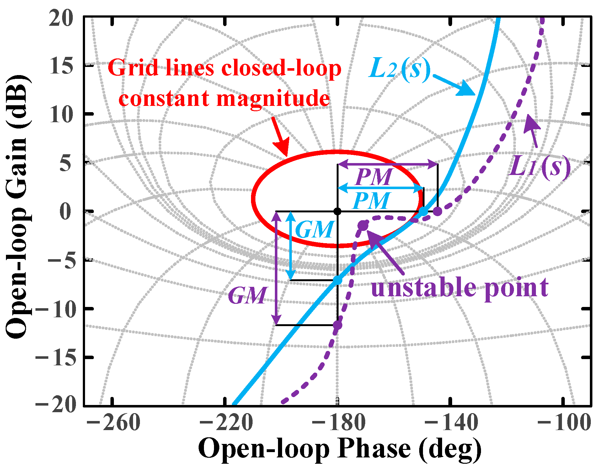
Traditional GM and PM impose constraints only at a phase of −180 degree and gain of 0 dB, without covering the full-range frequency [33]. When multiple resonant modes exist in the plants, the single-point constraints defined by PM or GM are insufficient to ensure the overall stability, potentially leading to instability during loop gain scheduling. In Figure 2, even though the open-loop curve L₁(s) has higher PM and GM compared to L₂(s), it is very close to the point (0 dB, −180 degree). This indicates that the L₁(s) system has a higher resonance peak than the L₂(s) system, which can lead to severe vibrations and cause irreversible damage to the system.

Therefore, in this section, the stability constraint is extended to full-range frequency based on the preset PM and GM, which are treated as two independent variables to enable the precise definition of stability constraints in the medium- and high-frequency ranges, while providing sufficient flexibility for subsequent loop tuning to avoid redundancy.

Step 1: To facilitate constraint imposition, the analytical relationship between the closed-loop magnitude and margins is first derived. As a direct representation of system stability, the closed-loop magnitude reflects the resonance peak and bandwidth characteristics. Excessively high magnitude values can compromise system stability; therefore, a constant upper limit, W_thres (a constant value of 1 corresponds to 0 dB), is set to ensure system stability, yielding the following inequality:

$$|G_{cl}(j\omega )|=\left|{\displaystyle \frac{feedback\left(j\omega \right)}{reference\left(j\omega \right)}}\right|=\left|{\displaystyle \frac{L\left(j\omega \right)}{1+L\left(j\omega \right)}}\right|\le W_{thres}\hspace{1em}\forall \omega >0$$

(2)

According to the mathematical derivation in Appendix A, (2) can be rewritten as (3):

$${(X_L+{\displaystyle \frac{W_{thres}^2}{W_{thres}^2-1}})}^2+Y_L^2\ge {\left({\displaystyle \frac{W_{thres}}{W_{thres}^2-1}}\right)}^2$$

(3)

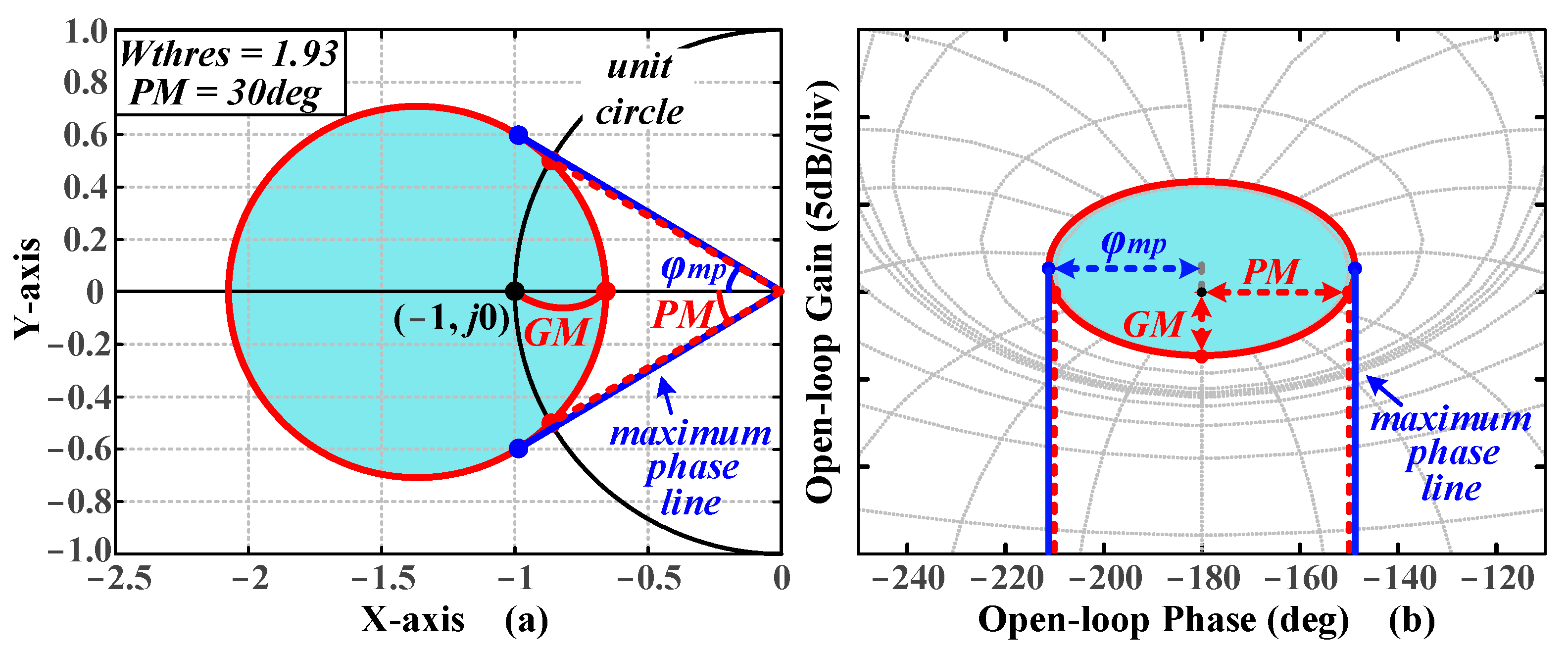
When (3) is satisfied with equality, it manifests as a circle in the Nyquist plot, denoted as O_cl. If the open-loop curve does not enter O_cl, the system satisfies the constraint of (2). Assuming W_thres = 1.93, the red circle in Figure 3 represents O_cl, with the blue area inside indicating the constraint region. The corresponding GM and PM are marked in Figure 3.

The intersection point of O_cl with the unit circle in the complex plane is (−cos(PM), −jsin(PM)), where the angle between (−cos(PM), −jsin(PM)) and the real axis represents PM. Thus, based on this point and (3), PM can be expressed as:

$$PM={\mathrm{c}\mathrm{o}\mathrm{s}}^{-1}\left({\displaystyle \frac{2W_{thres}^2-1}{2W_{thres}^2}}\right)$$

(4)

Therefore, based on the predefined PM, the first stability constraint boundary O_cl across the entire frequency range can be established through (3) and (4).

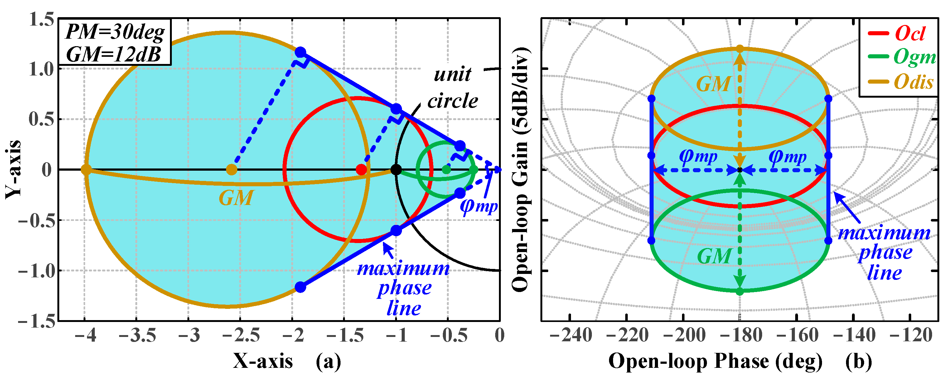
Step 2: When the resonant modes of plants are located in higher frequency ranges, the mid-frequency stability constraint defined by PM may fail to ensure sufficient stability margins in the high-frequency range (e.g., resonant points above 1 kHz caused by encoder installation issues). Hence, GM needs to be employed to extend the stability boundary in certain cases. To guide the extension operation, the ‘flat phase’ specification in [25] is referenced. This specification indicates that the PM remains unchanged, implying that the partial derivative of phase with respect to ω is zero, thereby ensuring the robustness of the control system to variations in loop gain. Hence, the stability boundary is extended rightward along the maximum phase line of O_cl to satisfy the ‘flat phase’ specification. The angle between the maximum phase line and the real axis is denoted as φ_mp, and is defined as follows:

$${\phi }_{mp} = {\sin }^{-1} ( \underset{\mathit{the} \mathit{radius} \mathit{of} \mathit{Ocl}}{\underbrace{{\displaystyle \frac{W_{thres}}{W_{thres}^2 - 1}}}} /\underset{\mathit{the} \mathit{center} \mathit{of} \mathit{Ocl}}{\underbrace{\left|-\frac{W_{thres}^2}{W_{thres}^2-1}\right|}})={\sin }^{-1}\left(\frac{1}{W_{thres}}\right)$$

(5)

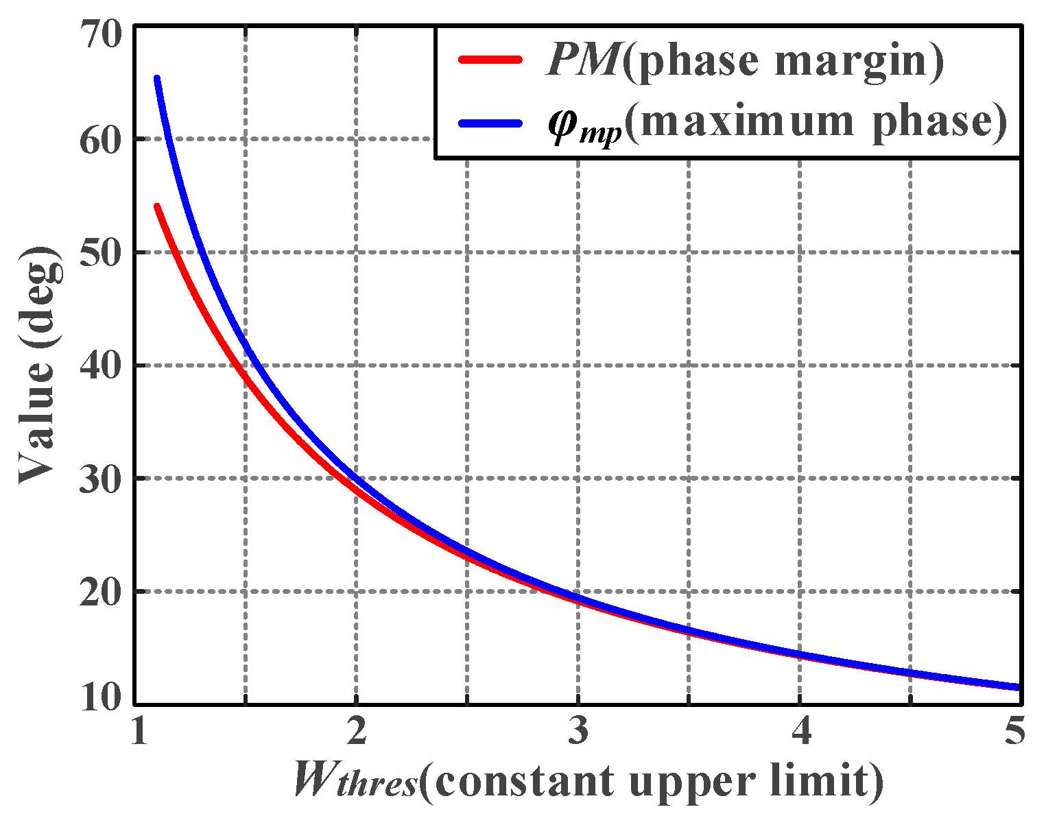
Replacing PM with φ_mp as part of the boundary ensures the improved continuity of the boundary phase. Moreover, given the small difference between PM and φ_mp in Figure 4, this replacement does not lead to an excessive stability margin.

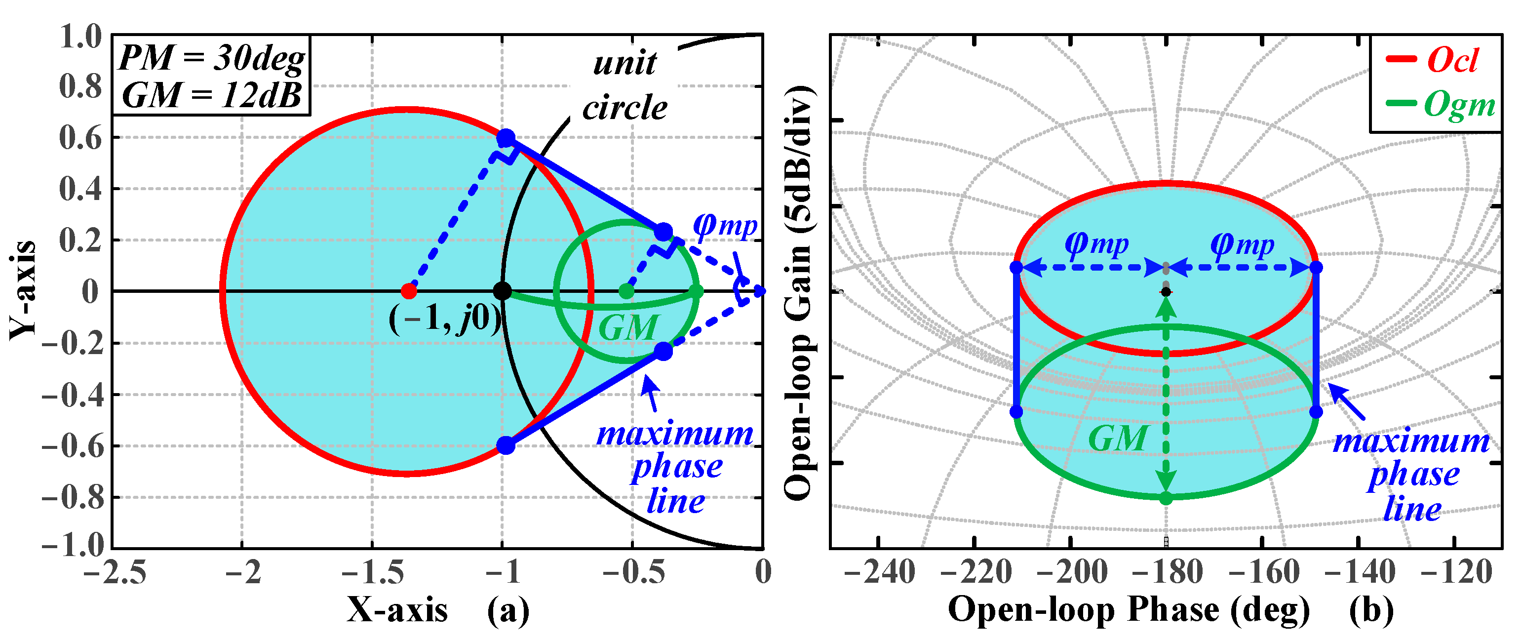
By shifting the O_cl rightward along the maximum phase line, a new circle O_gm is then obtained. O_gm must be tangent to the maximum phase line to satisfy the same phase constraints as the existing boundary. In addition, its proximal intersection with the real axis represents the preset GM, allowing the stability boundary corresponding to O_gm to be set by GM. The analytical expression of O_gm is then derived. The green circle in Figure 5 illustrates O_gm.

$$\begin{array}{cc}GM\hfill & =20{\mathrm{l}\mathrm{o}\mathrm{g}}_{10}\left(\left|-1\right|\right)-20{\mathrm{l}\mathrm{o}\mathrm{g}}_{10}\left(\left|-X_{O_{gm}}\right|\right)\hfill \\ \hfill & =-20{\mathrm{l}\mathrm{o}\mathrm{g}}_{10}\left(X_{O_{gm}}\right)\hfill \end{array}$$

(6)

where X_Ogm represents the magnitude of proximal intersection point (−X_Ogm, j0) between O_gm and the real axis. The distance from (−X_Ogm, j0) to (−1, j0) is equal to the adjustable variable GM.

This calculation yields X_Ogm = ${10}_1^{-GM/20}$. Then, the radius and the center of O_gm are defined as R_Ogm and (${-10}_1^{-GM/20}$ − R_Ogm, j0), respectively. Based on the similar triangles in Figure 5a, the following can be obtained from (5):

$${\phi }_{mp}={\mathrm{s}\mathrm{i}\mathrm{n}}^{-1}(R_{Ogm}/\underset{ the center of \mathrm{O}gm}{\underbrace{|-10^{-{\displaystyle \frac{GM}{20}}}-R_{Ogm}|}})={\mathrm{s}\mathrm{i}\mathrm{n}}^{-1}\left({\displaystyle \frac{1}{W_{thres}}}\right)$$

(7)

where

$$R_{Ogm}={\displaystyle \frac{10^{-\frac{GM}{20}}}{W_{thres}-1}}$$

(8)

Based on the radius R_Ogm in (8) and the center of O_gm, the analytical expression of O_gm is given as:

$$(X_L+{\displaystyle \frac{W_{thres}}{W_{thres}-1}}·10^{-{\displaystyle \frac{GM}{20}}})+Y_L^2={\left({\displaystyle \frac{10^{-\frac{GM}{20}}}{W_{thres}-1}}\right)}^2$$

(9)

The blue region in Figure 5a represents the final closed-loop magnitude constraint for stability, while Figure 5b illustrates the corresponding pattern of this constraint in the Nichols plot.

2.3. Disturbance Rejection Constraint Boundary

Unlike the stability constraint in the medium- and high-frequency ranges, the disturbance rejection capability of the system places greater emphasis on the low-frequency range. Thus, this part constructs a new circle, O_dis, representing the disturbance rejection constraint boundary based on the preset GM and the maximum phase line. Firstly, the sensitivity function [30] is introduced to evaluate the system’s response to low-frequency disturbances, and its expression is as follows:

$$\left|{\displaystyle \frac{error\left(j\omega \right)}{reference\left(j\omega \right)}}\right|={\displaystyle \frac{1}{|1+L(j\omega \left)\right|}}$$

(10)

where |1 + L(jω)| represents the distance from the open-loop curve to the point (−1, j0) in the complex plane. This implies that the disturbance rejection performance of the system can be enhanced by increasing the value of |1 + L(jω)|.

Despite the fact that O_dis is designed to increase the value of |1 + L(jω)| in the low-frequency range, it must meet the phase constraint of the existing stability boundary to ensure the phase continuity of the boundary. Thus, O_dis is set tangent to the maximum phase line. The brown circle in Figure 6a illustrates O_dis.

Define the distal intersection between O_dis and the real axis as (−X_Odis, j0), and set the distance from (−X_Odis, j0) to (−1, j0) to be equal to the preset GM. Therefore, X_Odis satisfies:

$$\begin{array}{cc}GM\hfill & =20{\mathrm{l}\mathrm{o}\mathrm{g}}_{10}\left(\right|-X_{Odis}\left|\right)-20{\mathrm{l}\mathrm{o}\mathrm{g}}_{10}\left(\right|-1\left|\right)\hfill \\ \hfill & =20{\mathrm{l}\mathrm{o}\mathrm{g}}_{10}\left(X_{Odis}\right)\hfill \end{array}$$

(11)

This calculation yields X_Odis = ${10}_1^{-GM/20}$. Then, the radius and the center of O_dis are defined as R_Odis and (−${10}_1^{-GM/20}$ + R_Odis, j0), respectively. Based on the similar triangles in Figure 6a, the following can be derived from (5):

$${\phi }_{mp}={\mathrm{s}\mathrm{i}\mathrm{n}}^{-1}(R_{Odis}/\underset{ the center of Odis}{\underbrace{|R_{Odis}-10^{{\displaystyle \frac{GM}{20}}}|}})={\mathrm{s}\mathrm{i}\mathrm{n}}^{-1}\left(\frac{1}{W_{thres}}\right)$$

(12)

where

$$R_{Odis}={\displaystyle \frac{10^{\frac{GM}{20}}}{W_{thres}+1}}$$

(13)

Based on the radius R_Odis in (13) and the center of O_dis, the analytical expression of O_dis is given as:

$$(X_L+{\displaystyle \frac{W_{thres}}{W_{thres}+1}}·10^{{\displaystyle \frac{GM}{20}}})+Y_L^2={\left({\displaystyle \frac{10^{\frac{GM}{20}}}{W_{thres}+1}}\right)}^2$$

(14)

By extending the maximum phase line and the stability constraint boundary leftward and connecting them with O_dis, the blue region in Figure 6a represents the final constraint boundary. Figure 6b shows the corresponding pattern in the Nichols plot. Thus far, the stability and disturbance rejection constraint boundaries together form the full-range frequency constraint boundary. Based on this, an automatic tuning algorithm for loop shaping is developed in the next part.

3. Proposed Automatic Tuning Algorithm

To achieve the desired system stability and dynamic response performance, an automatic tuning algorithm for loop shaping based on the constraint boundary is proposed in this section. The search algorithm first obtains all the controller parameter solutions that ensure that the system satisfies the preset constraints. Then, the local failure phenomena of some solutions are analyzed, and a validation algorithm is proposed to remove these solutions. Finally, a solution is selected to optimize the dynamic performance of the system.

3.1. Search Algorithm

When considering the dynamic response performance of the system, the optimal open-loop curve (the optimal solution of the controller) for the system under a specific constraint boundary must be tangent to the boundary in order to achieve a high closed-loop bandwidth and high dynamic response performance while ensuring the preset frequency-domain specifications.

The tangent point reflects the closed-loop resonance peak of the system; thus, the selection of the tangent point interval is critical to the system’s stability and closed-loop bandwidth. Since both stability and bandwidth are constrained by PM and GM, the O_gm boundary, defined by PM and GM, is selected as the tangent point interval. Therefore, the tangent point coordinates (X_B, jY_B) on the O_gm and the slope k_B of the tangent equation at (X_B, jY_B) can be expressed as:

$$\left\{\begin{array}{l}{X}_B=\underset{\mathit{the} \mathit{center} \mathit{of} \mathit{Ogm}}{\underbrace{-{\displaystyle \frac{W_{\mathit{thres}}}{W_{\mathit{thres}}-1}}\cdot {10}^{-{\displaystyle \frac{GM}{20}}}}}+\underset{\mathit{the} \mathit{radius} \mathit{of} \mathit{Ogm}}{\underbrace{{\displaystyle \frac{{10}^{-\frac{GM}{20}}}{W_{\mathit{thres}}-1}}}}\cdot \mathrm{c}\mathrm{o}\mathrm{s}\theta \\ Y_B=\underset{\mathit{the} \mathit{radius} \mathit{of} \mathit{Ogm}}{\underbrace{{\displaystyle \frac{{10}^{-\frac{GM}{20}}}{W_{\mathit{thres}}-1}}\cdot \mathrm{s}\mathrm{i}\mathrm{n}\theta }}\\ k_B=\mathrm{t}\mathrm{a}\mathrm{n}\left({\displaystyle \frac{\pi }{2}}+\theta \right)\end{array}\right.$$

(15)

where θ denotes the polar angle between the line from the center of O_gm to (X_B, jY_B) and the real axis, where the initial angle θ_start and terminal angle θ_end are (φ_mp − 0.5π) and 0π, respectively.

After obtaining X_B, Y_B, and k_B, the open-loop transfer function L(jω) for the given plant H(jω) = X_H(ω) + jY_H(ω), comprising a PI controller Gpi(jω) and a low-pass filter G_f(jω), which can be expressed as:

$$\{\begin{array}{c}{G}_f(j\omega ,{\omega }_0)=X_f(\omega ,{\omega }_0)+j{Y}_f(\omega ,{\omega }_0)\hfill \\ G_{pi}(j\omega )=K_p(1+{\displaystyle \frac{K_i}{j\omega }})=K_p-j{\displaystyle \frac{K_p{K}_i}{\omega }}\hfill \\ L(j\omega ,{\omega }_0)=G_f·G_{pi}·H=X_L(\omega ,{\omega }_0)+j{Y}_t(\omega ,{\omega }_0)\hfill \end{array}$$

(16)

where ω₀, X_f, and Y_f represent the cutoff frequency, real part, and imaginary part of the low-pass filter, respectively. Based on (16), the tangent point coordinates (X_L, jY_L) on the open-loop transfer function and the slope k_L of the tangent equation at (X_L, jY_L) can be expressed as:

$$\{\begin{array}{c}{X}_L=K_p(X_f{X}_H-Y_f{Y}_H)+{\displaystyle \frac{K_p{K}_i}{\omega }}(X_H{Y}_f+X_f{Y}_H)\hfill \\ Y_L=K_p(X_H{Y}_f+X_f{Y}_H)-{\displaystyle \frac{K_p{K}_i}{\omega }}(X_f{X}_H-Y_f{Y}_H)\hfill \\ k_L={\displaystyle \frac{d{Y}_L}{d{X}_L}}={\displaystyle \frac{d{Y}_L/d\omega }{d{X}_L/d\omega }}\hfill \end{array}$$

(17)

Appendix B provides the derivation of k_L. To formulate the analytical equation system for loop shaping, set k_B in (15) equal to k_L in (17), yielding (18a); equate the real and imaginary parts, X_B and Y_B in (14), with the corresponding X_L and Y_L in (17), resulting in (18b):

$$0=b_4{\omega }_0^4+b_3{\omega }_0^3+b_2{\omega }_0^2+b_1{\omega }_0^1+b_0$$

(18a)

$$\begin{array}{l}{K}_p={\displaystyle \frac{\left(X_f{X}_H-Y_f{Y}_H\right)X_B+\left(X_H{Y}_f+X_f{Y}_H\right)Y_B}{{\left(X_f{X}_H-Y_f{Y}_H\right)}^2+{\left(X_H{Y}_f+X_f{Y}_H\right)}^2}}\hfill \\ K_p{K}_i={\displaystyle \frac{\left(X_H{Y}_f+X_f{Y}_H\right)X_B-\left(X_f{X}_H-Y_f{Y}_H\right)Y_B}{{\left(X_f{X}_H-Y_f{Y}_H\right)}^2+{\left(X_H{Y}_f+X_f{Y}_H\right)}^2}}\omega \hfill \end{array}$$

(18b)

where b_i denotes the coefficient of ${\omega }_0^i$, which is a function of frequency ω and polar angle θ. Based on (18a) and (18b), the search algorithm for loop shaping can be derived, and the flowchart is shown in Figure 7.

Considering the impact of the modeling accuracy and algorithm execution time, the step θ_step and ω_step in Figure 7 can be set to 0.1 degree and 2.5 Hz, respectively. The same settings are applied in the following sections.

3.2. Validation Algorithm

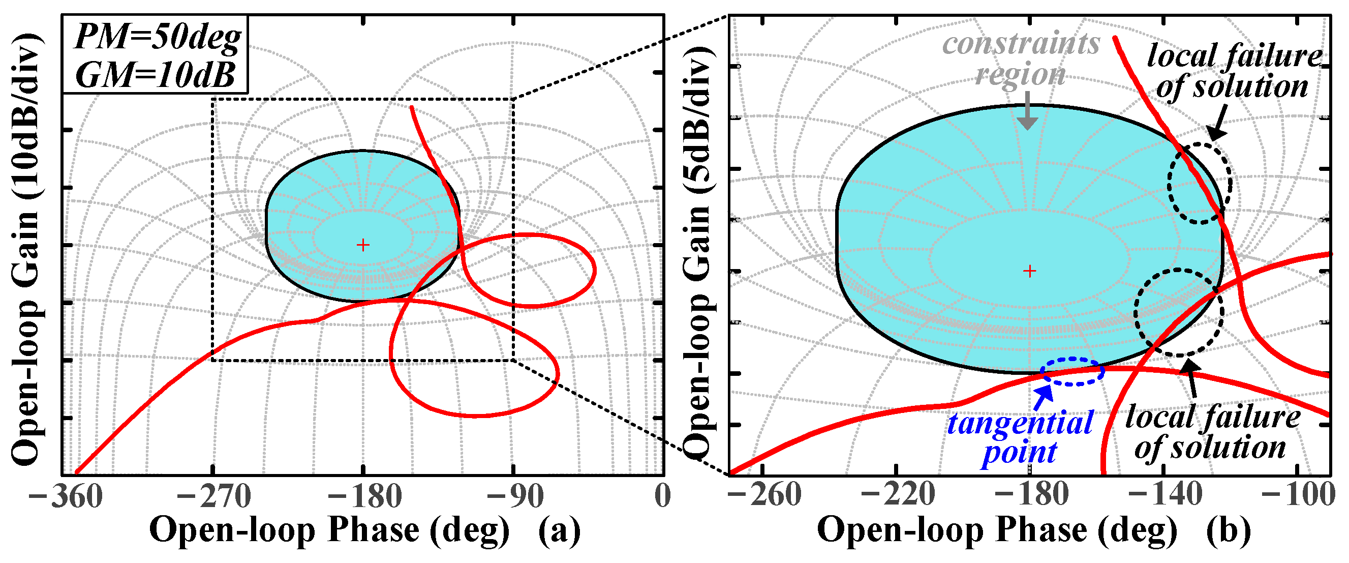
When the plant exhibits multiple resonance points, although the equation system (18) ensures that the system locally satisfies the predefined stability constraint at the tangent point, there remains a risk of violating the constraint within the ranges of other resonance points, leading to the failure of the solution. Figure 8 presents an example of a solution failure. Therefore, a validation algorithm is proposed to effectively remove solutions that lead to system instability.

To avoid an excessive execution time caused by verifying each frequency point, a frequency point should be verified only if it simultaneously satisfies the following:

• −π − φ_mp ∠L(jω_m) −π + φ_mp;
• Mmin |L(jω_m)| Mmax.

Where Mmin and Mmax represent the magnitudes of the proximal and distal intersections between the boundary and the real axis, respectively, in the complex plane. |L(jω_m)| and ∠L(jω_m) can be expressed as:

$$\angle L\left(j\omega \right)={\mathrm{t}\mathrm{a}\mathrm{n}}^{-1}(Y_L/X_L)$$

(19)

$$\left|L\right(j\omega \left)\right|=\sqrt{X_L^2+Y_L^2}$$

(20)

Based on (19) and (20), the flowchart of the proposed validation algorithm is shown in Figure 9, where y represents the number of solutions in the set Γ obtained from the search algorithm.

3.3. Final Solution Selection

After ensuring that the system meets the predefined stability and disturbance rejection constraints, the final solution is selected to optimize the dynamic performance of the system and maximize the closed-loop bandwidth ω_bw. The closed-loop magnitude M_cl(ω) can be expressed as:

$$M_{cl}(\omega )={(1+{\displaystyle \frac{1}{\left|L\right(j\omega ){|}^2}}+{\displaystyle \frac{2\mathrm{c}\mathrm{o}\mathrm{s}(\angle L(j\omega \left)\right)}{\left|L\right(j\omega \left)\right|}})}^{-{\displaystyle \frac{1}{2}}}$$

(21)

Regarding the discreteness of the data, the bandwidth ω_bw is defined as the median value between the two adjacent points at the first 0.707 (corresponding to −3 dB) crossover frequency, that is, (ω_m + ω_m−1)/2, where ω_m = ω_m−1 + ω_step. The bandwidth recording process can be synchronized with the validation algorithm, as shown in the red box in Figure 9, where bw denotes the bandwidth-recording flag.

To summarize, the proposed search and validation algorithm converts the preset closed-loop magnitude, gain, and phase margins into the desired dynamic performance and computes the corresponding controller parameters.

4. Experimental Validation on Different Platforms

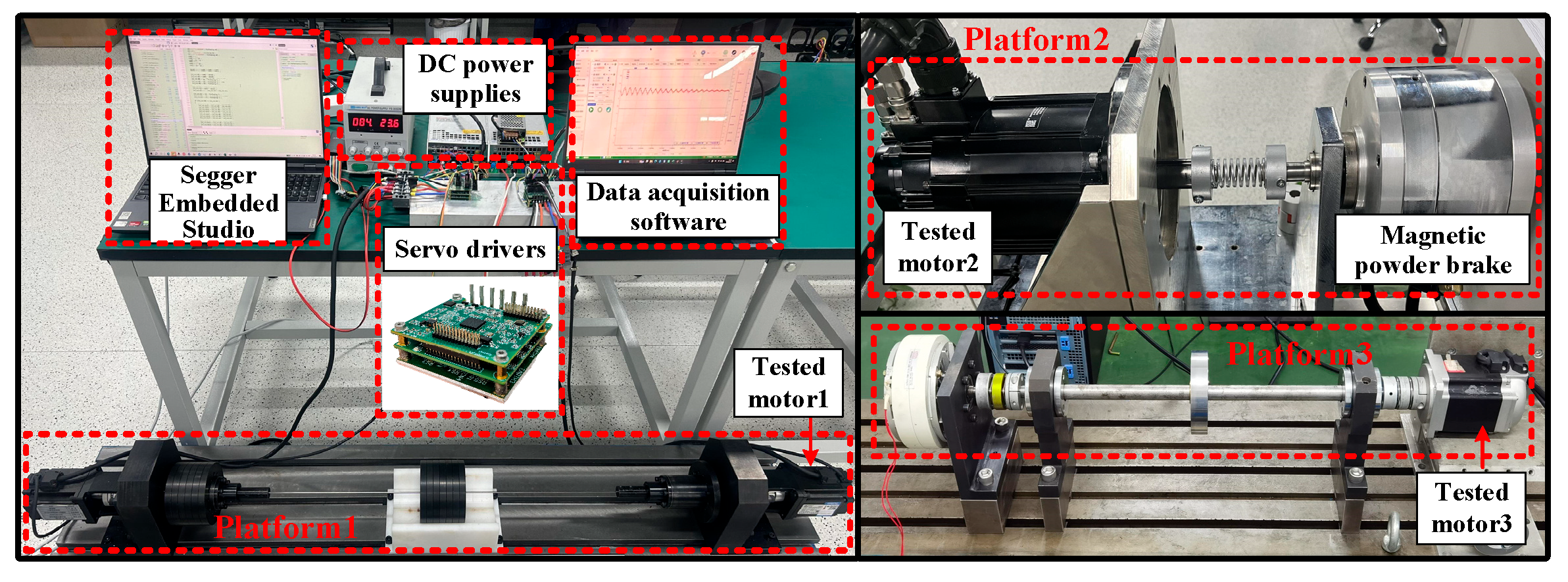
The subsequent experiments are carried out within the framework of the servo speed-loop system. To thoroughly validate the effectiveness of the algorithm, three mechanical platforms are utilized. The key parameters of the controller and tested motors are shown in

Table 1. Key parameters of the software platforms.

Key Parameter	Values
Controller Switching Frequency	10 kHz
Controller Sampling Frequency	5 kHz
Initial Frequency ωstart	5 Hz
Final Frequency ωend	1.25 kHz
Step frequency ωstep	2.5 Hz
Step angle θstep	0.1 degree

and

Table 2. Key parameters of the hardware platforms.

Key Parameter	Motor 1	Motor 2	Motor 3
Stator resistance	0.053 Ω	0.156 Ω	0.162 Ω
D–q axis inductance	0.102 mH	0.074 mH	0.285 mH
Rated torque	2.39 N·m	1.92 N·m	0.32 N·m
Rated current	7.07 A	6.54 A	6.06 A
Rated speed	3000 rpm	2800 rpm	2500 rpm
Power	750 W	600 W	135 W
Motor inertia	1.62 × 10−4 kg·m2	6.15 × 10−4 kg·m2	10.1 × 10−4 kg·m2
Pole pairs	8	4	5

, respectively. Figure 10 illustrates the experimental platform utilized in this paper, which includes two PCs, two self-developed servo drivers, multiple DC power supplies, and a magnetic powder brake. The self-developed servo drivers are based on the RISC-V microcontroller HPM6264 (HPMicro, Shanghai, China). Input commands are provided by the PC-side software (Xien Servo Driver Studio V1.1.071), while output data are collected by the upper computer software via RS-232.

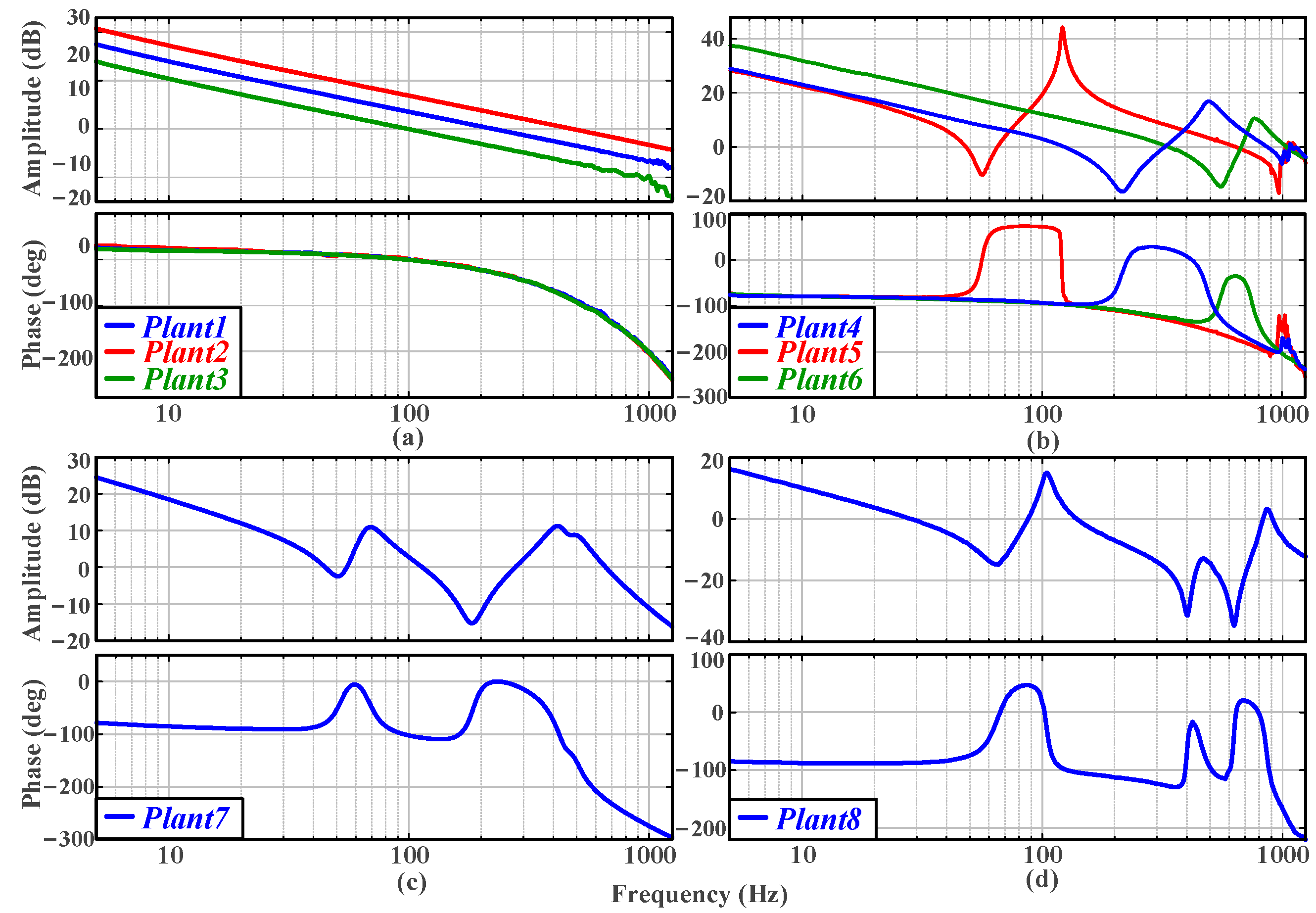
A zero-DC offset chirp signal is injected as the speed input for the frequency sweep, with the key parameter values of the software platforms recorded in Table 1. This results in the frequency set Ω containing 498 data points. The raw data collected are smoothed by the Hample filter, the Savitzky–Golay filter, and the Gaussian filter [34]. The resulting frequency characteristics of the plant are shown in Figure 11.

In Platform 1, both the tested motor and the load motor are implemented using Motor 1 in Table 2, and they are connected via a flexible shaft. By attaching different numbers of inertia disks to the motor and load sides, three distinct frequency characteristics of the plants are obtained, as illustrated in Figure 11b. In Platform 2, the tested motor is Motor 2 listed in Table 2, and the load side consists of a magnetic powder brake. The two components are connected via an elastic shaft. The frequency characteristic of the plant in Platform 2 is shown in Figure 11c. In Platform 3, the tested motor is Motor 3 listed in Table 2, and it is connected to the load side through multiple couplings and inertia disks. The frequency characteristic of the plant in Platform 3 is shown in Figure 11d. Figure 11a presents the frequency characteristics of Motors 1–3.

4.1. Comparison of Time-Domain Metrics Under Varying Preset Frequency-Domain Specifications

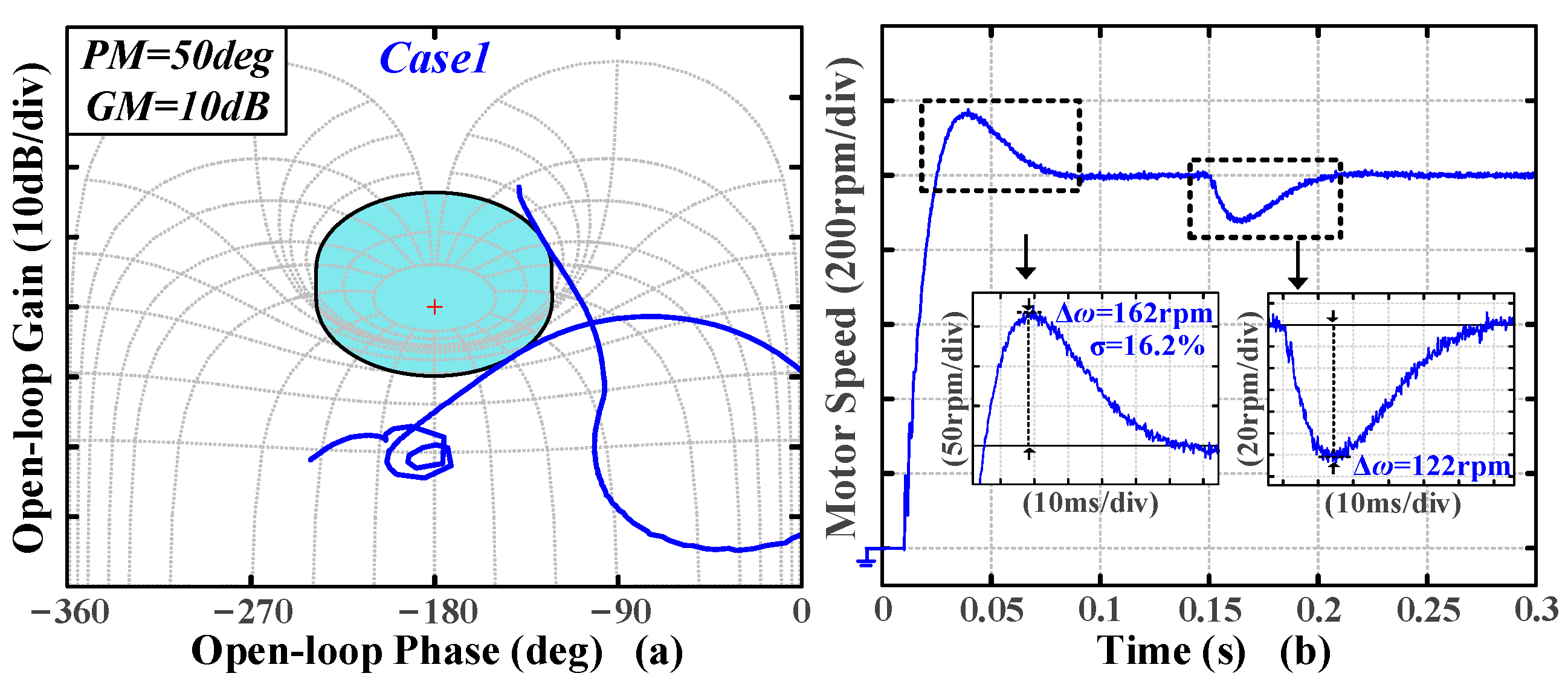
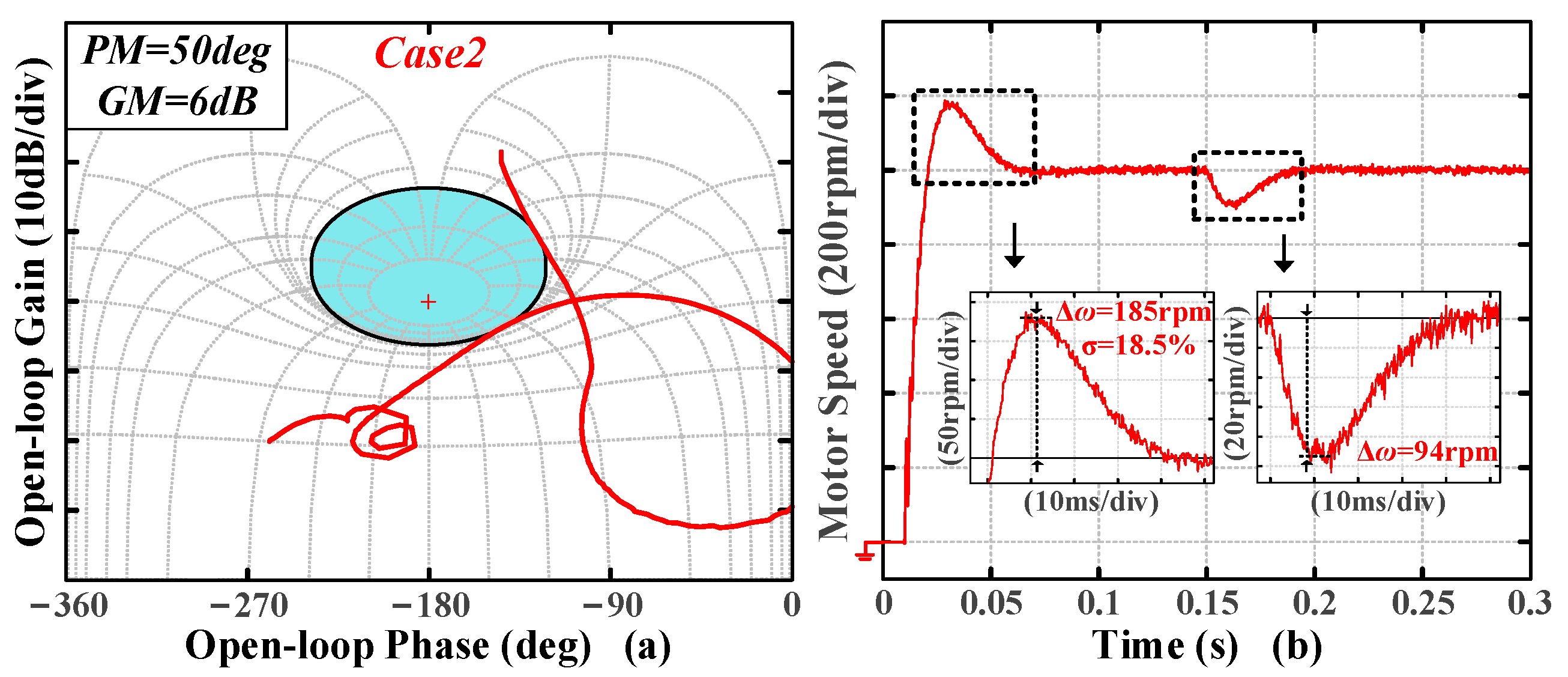
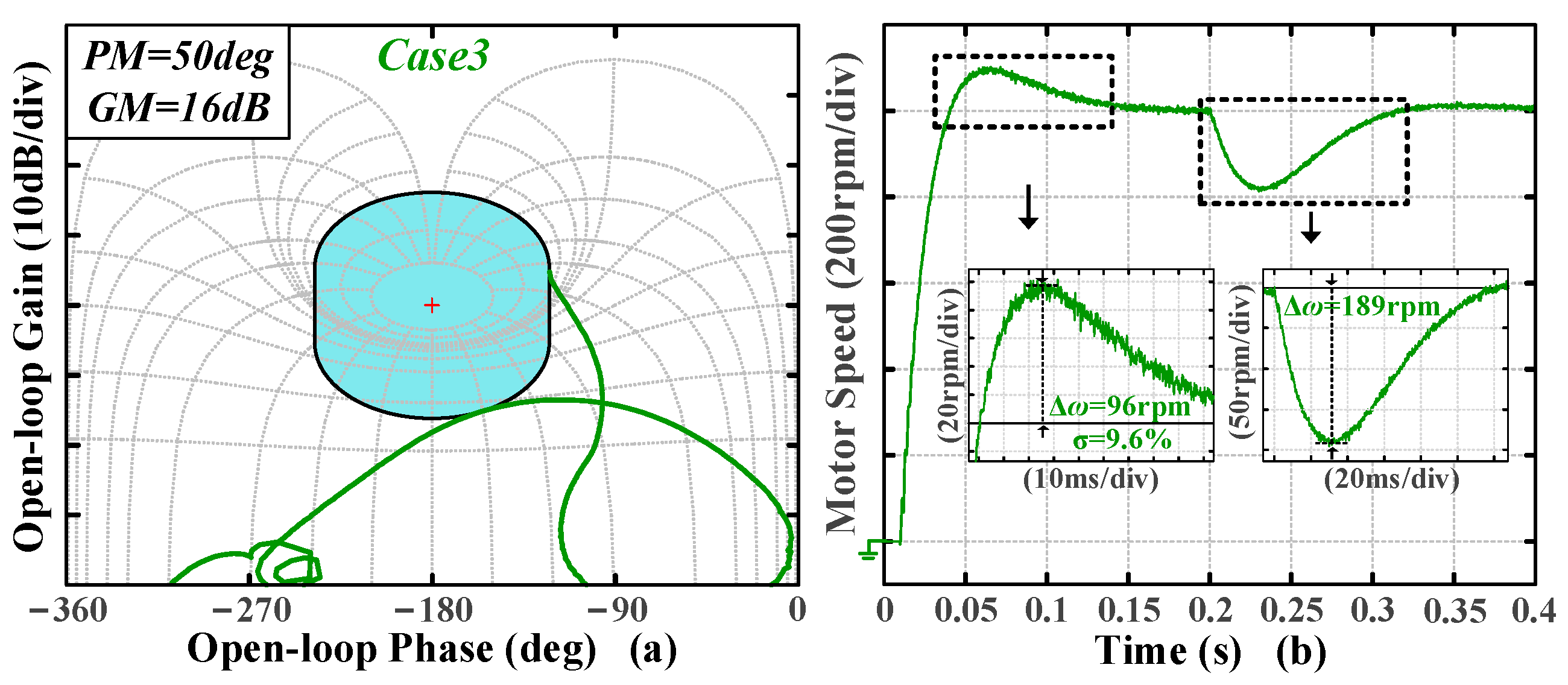
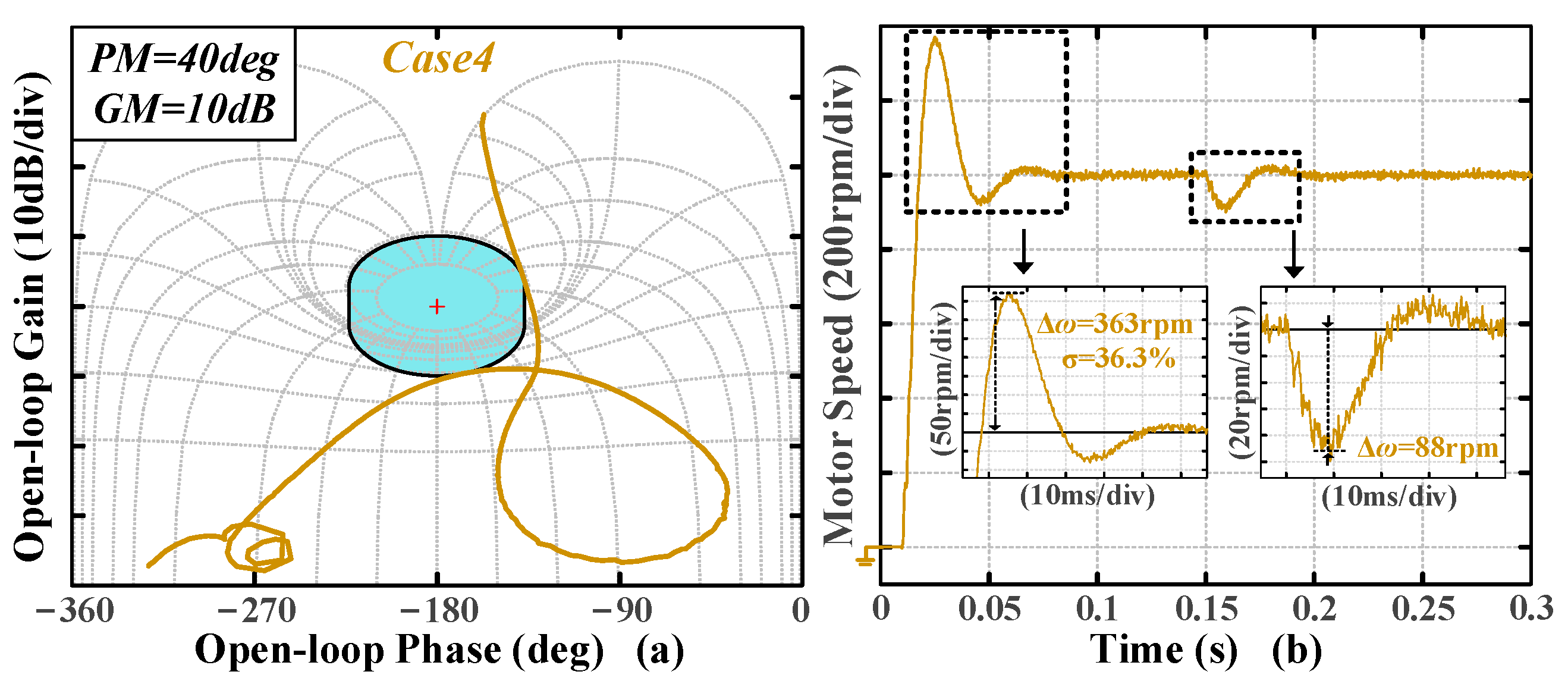
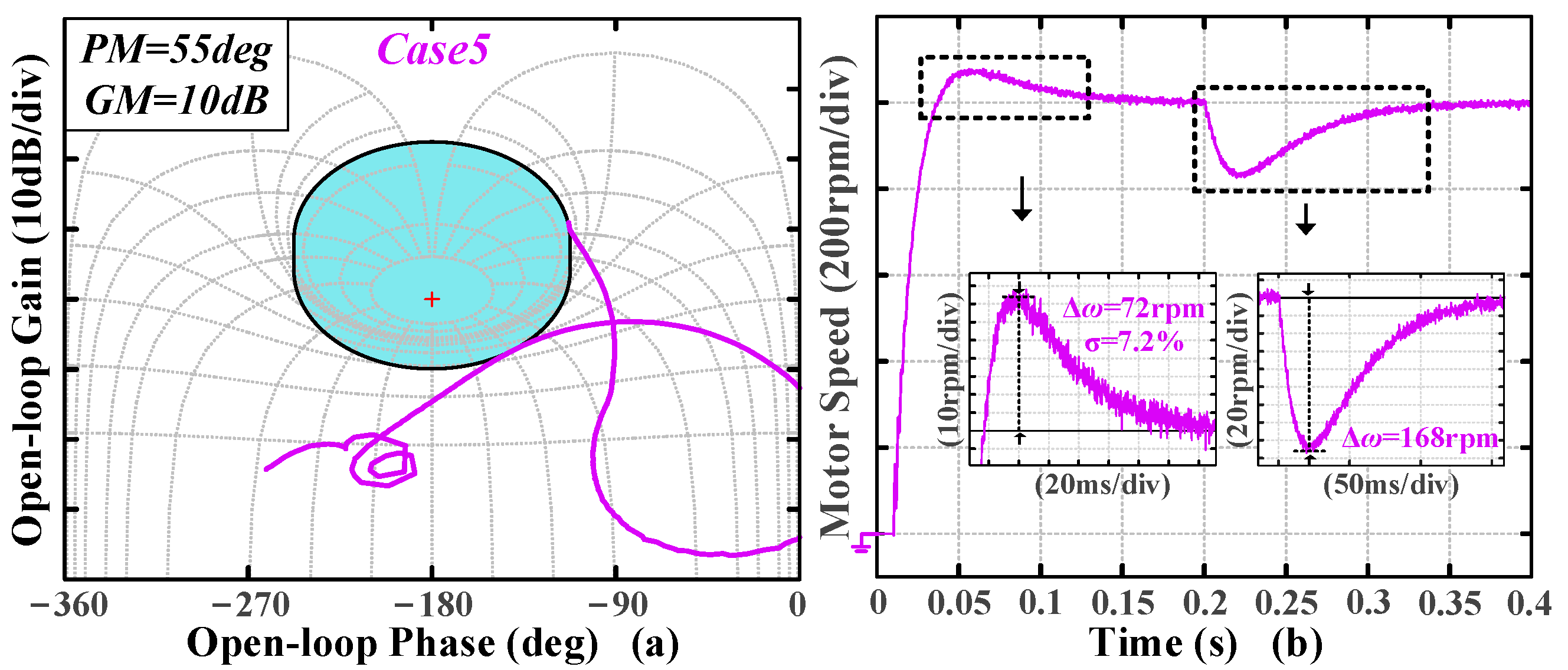
Plant 4 in Figure 11b is selected for the experiment. Different margin groups are set as the search algorithm inputs, with Case 1: PM = 50 degree and GM = 10 dB serving as the benchmark. Based on the benchmark, Case 2 and Case 3 reduce and increase the GM, respectively, while Case 4 and Case 5 reduce and increase the PM, respectively (

Table 3. The correspondence between different cases and stability margins.

Case	PM (Phase Margin)/deg	GM (Gain Margin)/dB
Case 1	50	10
Case 2	50	6
Case 3	50	16
Case 4	40	10
Case 5	55	10

). The Nichols plots of the tuning results under different cases are shown in Figure 12a, Figure 13a, Figure 14a, Figure 15a and Figure 16a.

The tuning results are presented in

Table 4. Tuning results for different preset frequency-domain specifications.

PM and GM	Tuning Results of Plant 4 Under Different PM and GM Values
	(Kp, Ki, ω0 (rad/s))	ωbw (Hz)	Overshoot (%)	Settling Time (s)	Speed Drop (%)	Recovery Time (s)
PM: 50 deg, GM: 10 dB	(0.121, 57, 31,501)	30.5	16.2	6.909 × 10−2	12.2	5.354 × 10−2
PM: 50 deg, GM: 6 dB	(0.163, 75, 21,247)	31.6	18.5	5.032 × 10−2	9.4	3.941 × 10−2
PM: 50 deg, GM: 16 dB	(0.045, 32, 2915)	9.7	9.6	1.437 × 10−1	18.9	1.164 × 10−1
PM: 40 deg, GM: 10 dB	(0.167, 155, 992)	46.3	36.3	6.664 × 10−2	8.8	3.926 × 10−2
PM: 55 deg, GM: 10 dB	(0.098, 23, 18,707)	15.5	7.2	1.551 × 10−1	16.8	1.569 × 10−1

. To acquire the corresponding time-domain metrics, transient experiments are conducted: a 1000 rpm step signal is applied at 0.01 s, followed by an abrupt torque of 0.3 pu load. The speed response waveforms under different cases are shown in Figure 12b, Figure 13b, Figure 14b, Figure 15b and Figure 16b. For ease of comparison, Figure 17 summarizes the speed response waveforms, categorizing them into varying gain margin groups and varying phase margin groups.

As shown in Table 4 and Figure 12b, Figure 13b, Figure 14b, Figure 15b and Figure 16b, an increase in either PM or GM individually results in a decrease in system overshoot, an increase in speed drop, and longer settling and recovery times. In addition, the corresponding closed-loop bandwidth is also reduced. In Figure 17, it is obvious that the time-domain metrics are influenced by both PM and GM, with their trends remaining consistent; specifically, a notable reduction in overshoot occurs with changes to either PM or GM independently. The experimental results indicate that the algorithm effectively transforms the preset stability and disturbance rejection specifications into the desired time-domain response.

4.2. Comparison of Time-Domain Metrics Under Different Types of Plants

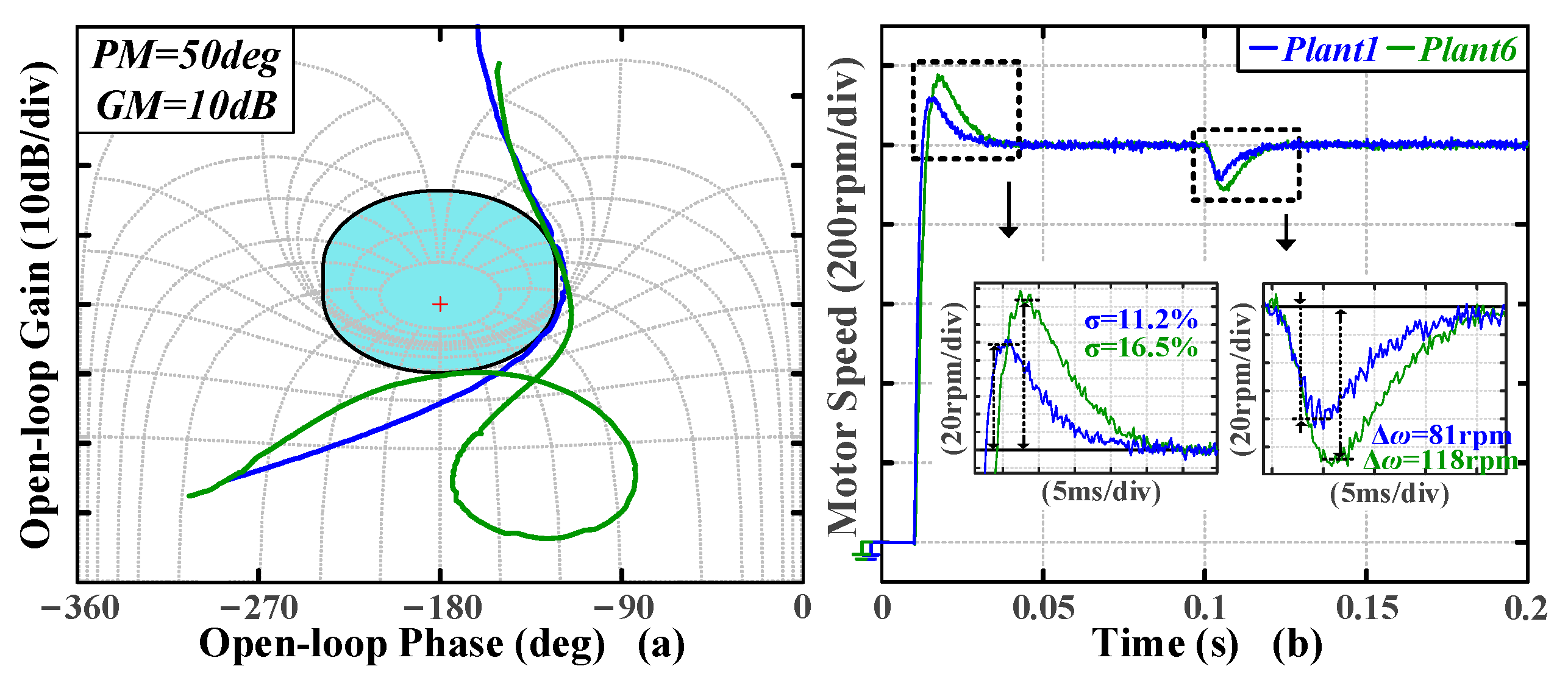
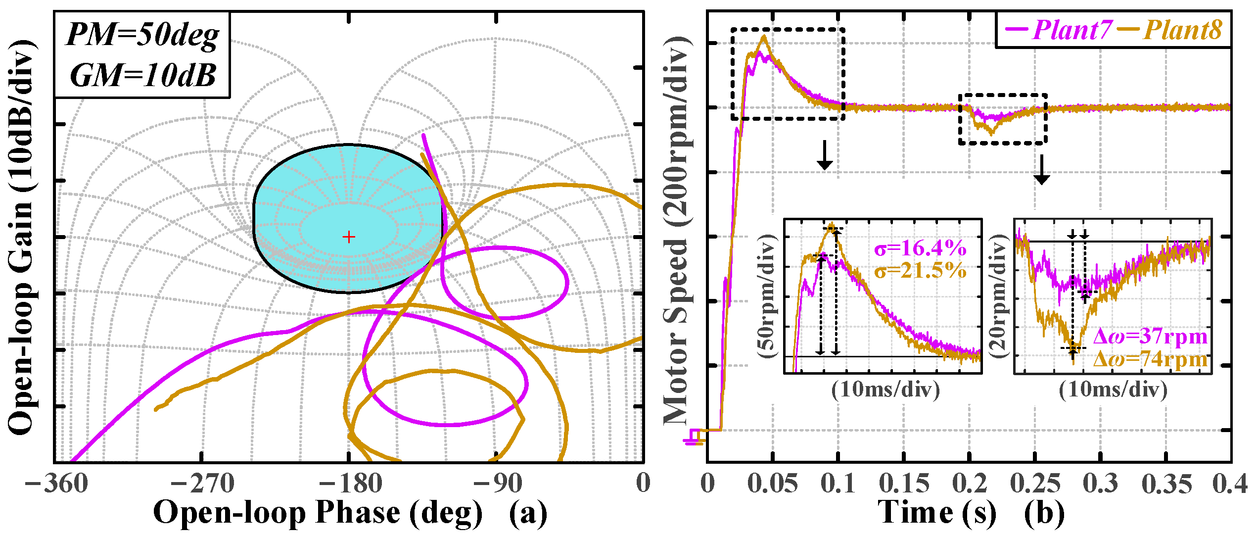
To validate the versatility of the algorithm, different types of plants—plant 1, plant 5, plant 7, and plant 8 in Figure 11—are selected for the experiments. The experiments are conducted based on the benchmark. The Nichols plots of the tuning results are shown in Figure 18a and Figure 19a. The same transient experiments as the last part are conducted to obtain the time-domain metrics. The speed waveforms are shown in Figure 18b and Figure 19b. Figure 20 presents the corresponding closed-loop magnitude Bode plot.

As shown in Figure 18b and Figure 19b, the tested plants—plant 1, plant 6, plant 7, and plant 8—exhibit distinct time-domain metrics under the same Case1 margin inputs. This is primarily attributed to the significant differences in their frequency characteristics, as these plants differ in system order, leading to variations in overshoot, speed drop, settling, and recovery time. The tuning results for different plants are summarized in

Table 5. Tuning results for different plants.

Plant	Tuning Results Under PM: 50 deg, GM: 10 dB
	(Kp, Ki, ω0 (rad/s))	ωbw (Hz)
plant 1	(0.242, 143, 6097)	217.2
plant 2	(0.502, 151, 5784)	208.4
plant 3	(1.242, 165, 7428)	228.6
plant 4	(0.121, 57, 31,501)	30.5
plant 5	(0.165, 67, 11,539)	25.7
plant 6	(0.152, 144, 3797)	95.8
plant 7	(0.283, 41, 549)	22.1
plant 8	(0.532, 36, 1802)	27.4

. It is obvious that the closed-loop bandwidth of the obtained system is limited by the inherent anti-resonance frequencies of the plants, leading to variations in the settling and recovery times. Despite the differences, the settling and recovery times of different plants are consistent with their anti-resonance frequencies. Inertial systems (plants 1–3) exhibit higher closed-loop bandwidths compared to other systems.

4.3. Comparison of Time-Domain Metrics Under Identical Types of Plants

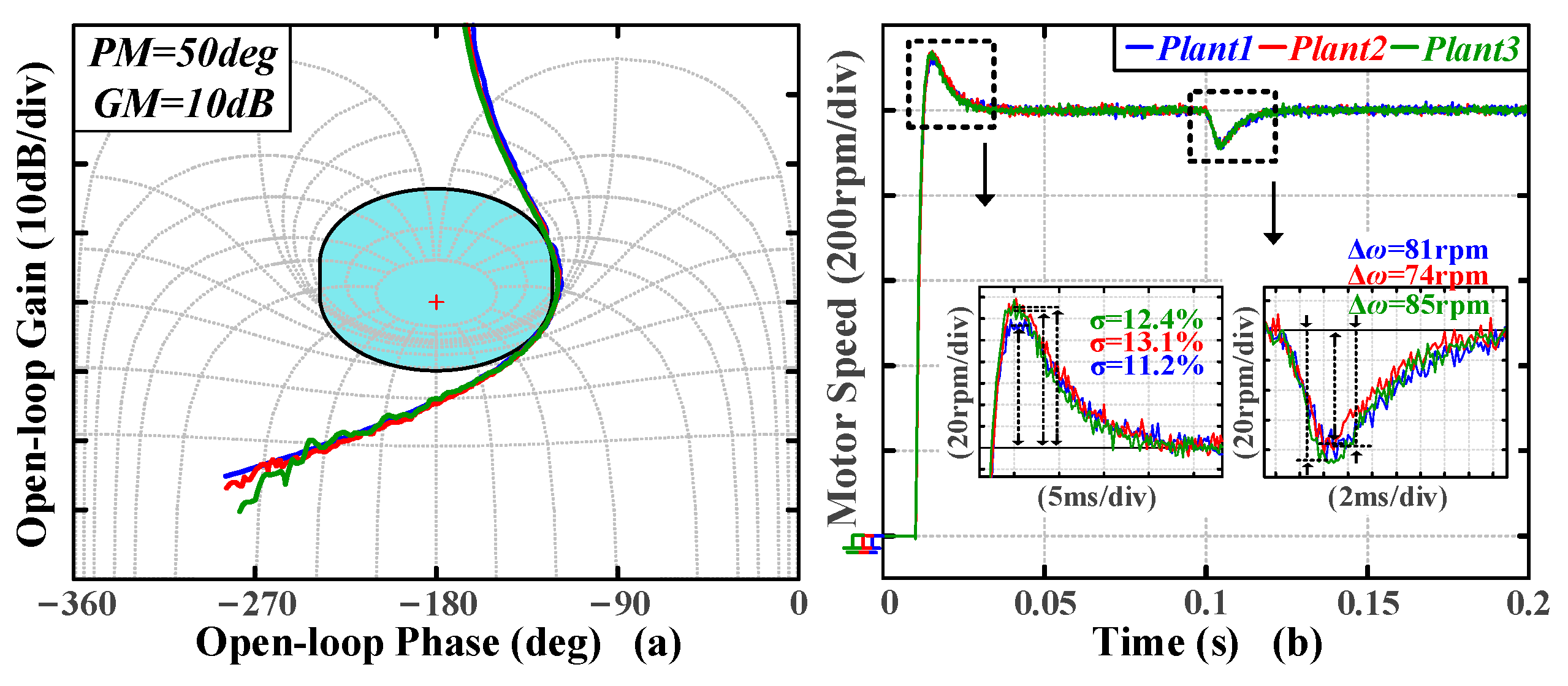
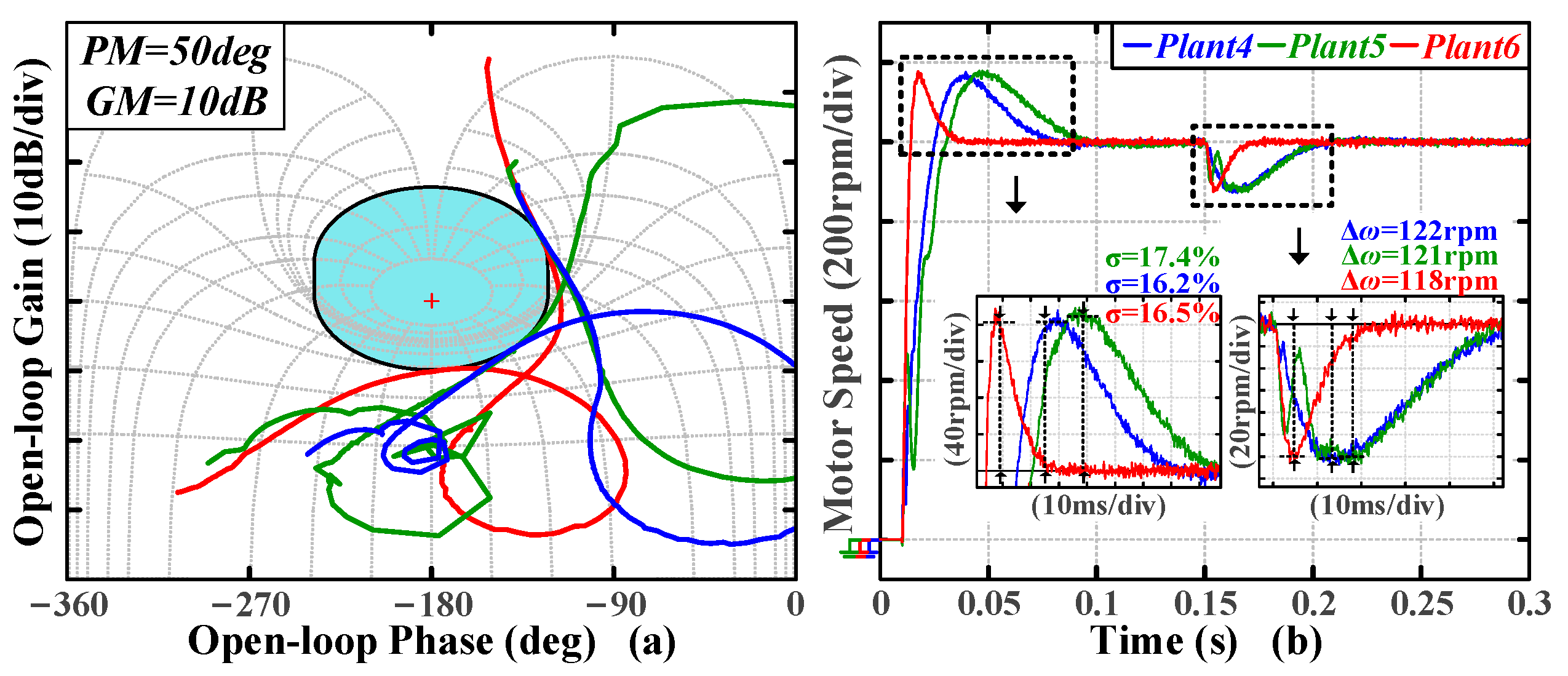
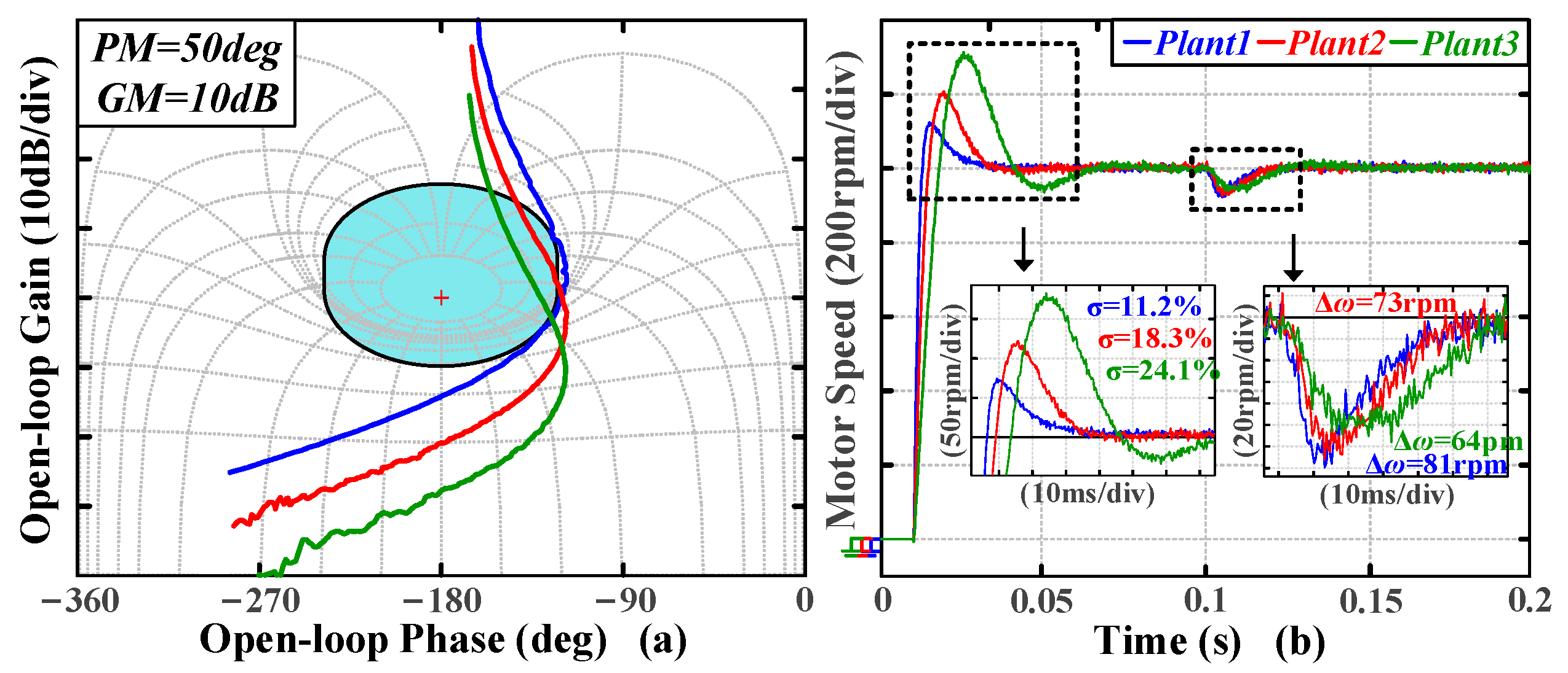
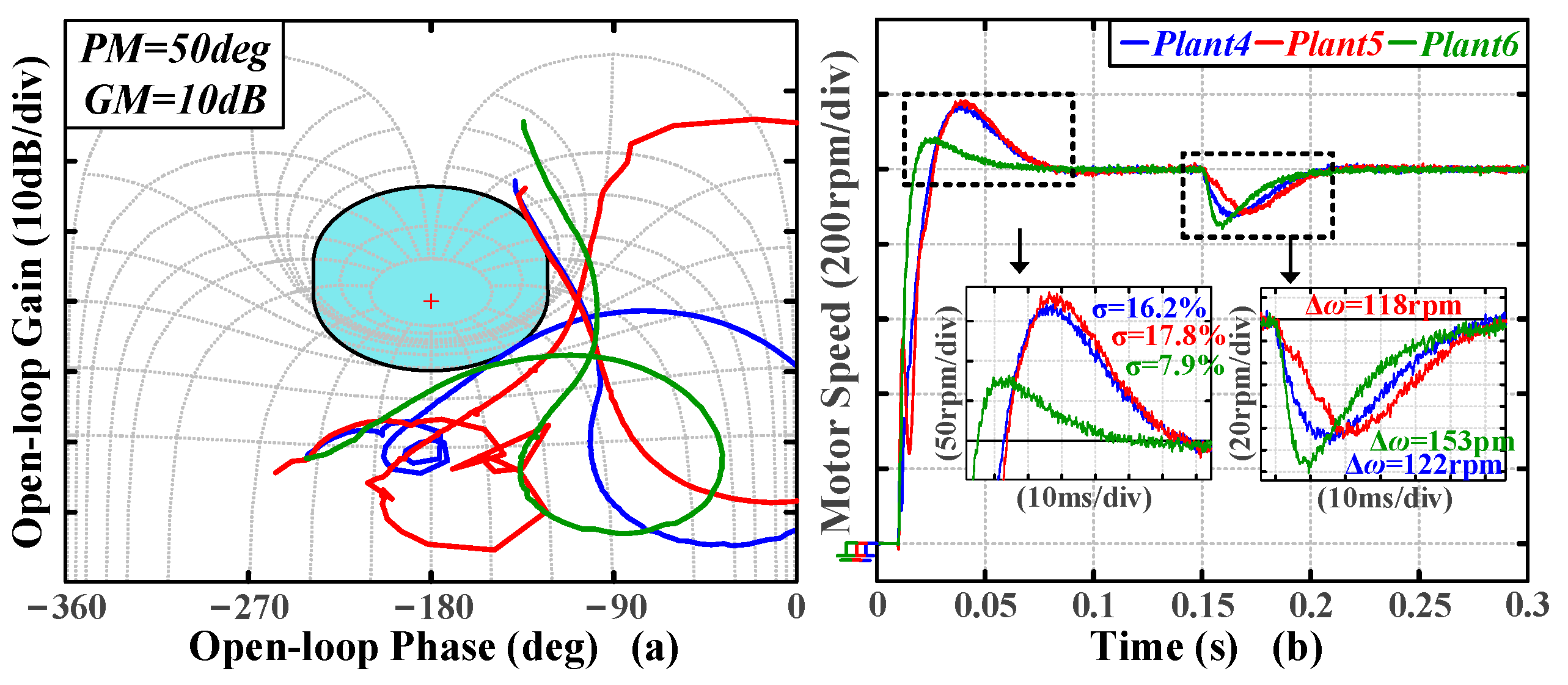
To further explore the relationship between frequency-domain and time-domain metrics under different plants, three inertial systems in Figure 11a and three single resonance point systems in Figure 11b are used for experiments, respectively. The experiments are conducted based on the benchmark. The Nichols plots of the tuning results are shown in Figure 21a and Figure 22a. The same transient experiments as the last part are conducted to obtain the time-domain metrics. The speed waveforms are shown in Figure 21b and Figure 22b.

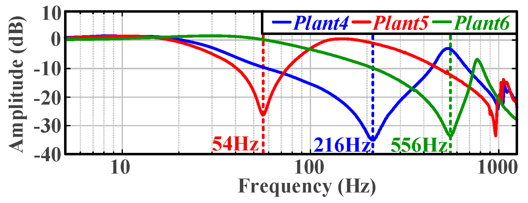
In Figure 21b, the time-domain metrics for inertial systems exhibit consistency: the maximum differences in overshoot and speed drop are 1.9% and 1.1%, respectively. In Figure 22b, the maximum differences in overshoot and speed drop are 1.2% and 0.4%, respectively. Given the differences in the inherent anti-resonant points of the single-resonance point systems, which limit the closed-loop bandwidth in Figure 23, settling and recovery times are consistent with anti-resonance frequencies.

In summary, the proposed algorithm converts the preset PM and GM into the desired dynamic performance, as validated by the experimental time-domain metrics, which vary with changes in PM and GM. In addition, the algorithm presents compatibility with different types of plants, with the tuned systems exhibiting excellent transient performance. Furthermore, for plants with the same number of resonance points, the tuning results exhibit a certain degree of consistency in overshoot and speed drop. The differences in settling and recovery times can be correlated with the anti-resonance frequencies of the plants.

4.4. Comparison of Time-Domain Metrics with Systems Tuned by ZPC

To demonstrate the advantages of the proposed tuning algorithm, a comparison is conducted between the proposed method and the zero-pole cancellation (ZPC) strategy, where ZPC is implemented following reference [35]. As a foundation, the speed servo block diagram and calculation formulas used for ZPC are first introduced.

In Figure 24, Ksp and Ksi represent the proportional and integral gains of the speed controller, respectively, while Kcp and Kci represent the proportional and integral gains of the current loop controller, respectively. L and R denote the stator inductance and q-axis resistance of the motor, respectively; J represents the motor inertia; and K_T denotes the torque constant. When the current loop bandwidth is sufficiently high, its closed-loop transfer function can be approximated as 1.

$$\{\begin{array}{c}{G}_{so}(s)={\displaystyle \frac{K_T{K}_{sp}{K}_{si}}{J{s}^2}}·({\displaystyle \frac{s}{K_{si}}}+1)\\ G_{sc}(s)={\displaystyle \frac{K_T{K}_{sp}(K_{si}+s)}{K_T{K}_{sp}(K_{si}+s)+J{s}^2}}\end{array}$$

(22)

where Gsc(s) and Gsc(s) denote the open-loop and closed-loop transfer functions of the speed control system, respectively.

$$\{\begin{array}{c}{K}_{si}={\omega }_{sc}/u\hfill \\ K_{sp}=J{\omega }_{sc}/K_T\hfill \end{array}$$

(23)

where ωsc denotes the speed loop gain crossover frequency and u denotes the preset phase margin. According to reference [35], by specifying the gain crossover frequency and phase margin of the open-loop transfer function of the system, along with the motor inertia, the parameters of the PI controller can be determined. With the gain crossover frequency set at 100 rad/s and the phase margin specified as 50 deg, the resulting PI controller parameters for Motors 1–3 are summarized in

Table 6. PI parameters for plants 1–3.

PI Parameter	Plant 1	Plant 2	Plant 3
Ksp	0.25	0.40	0.72
Ksi	132	157	174

.

In order to conduct a quantitative comparison with the tuning algorithm proposed in this paper, the stability margins used as inputs for the proposed algorithm are Case 1: PM = 50 deg, GM = 10 dB. To acquire the corresponding time-domain metrics, transient experiments are conducted: a 1000 rpm step signal is applied at 0.01 s, followed by an abrupt torque of 0.3 pu load at 0.1 s. The speed response curves of the experiment are shown in Figure 25.

As shown in Figure 25a–c, the system tuned using the ZPC-based method exhibits a larger overshoot and speed drop, as well as longer settling and recovery times compared to the proposed method. The comparison of the four time-domain performance metrics demonstrates that the tuning approach presented in this paper provides superior performance. The ZPC method is primarily designed for relatively simple PI controllers, which involve only two tunable parameters. In contrast, the controller employed in this paper adopts a PI filter structure with three tunable parameters. Therefore, the ZPC and the tuning algorithm proposed in this manuscript are developed for different controller structures, each requiring distinct types of input parameters.

4.5. Comparison of the Time-Domain Metrics of Different Order Systems Under Load Variation

To investigate the robustness of the proposed tuning algorithm against load variations, plant1 and plant4, representing two different types of systems, are, respectively, selected as the initial plants for tuning. Plants 2–3 and plants 5–6 are used as the plants after the inertia changes. The result for plant1’s controller parameters (K_p, K_i, and ω₀) is (0.242, 144, 6097); the result for plant4’s controller parameters is (0.121, 57, 31,501).

When the load of the inertia system changes, the corresponding open-loop curves are shown in Figure 26a. The curves cross the preset boundary, indicating that the stability and disturbance rejection constraints are no longer satisfied. The corresponding speed response waveforms are shown in Figure 26b, where the overshoot increases from 11.2% to 24.1%, and the settling time also changes accordingly. In contrast, when the load of the single-resonant system changes, the open-loop curve moves away from the boundary, resulting in excessive stability margins. As shown in Figure 27 and

Table 7. Time-domain metrics of transient response experiments.

Plant	Time-Domain Metrics of Transient Response Experiments
	ωbw (Hz)	Overshoot (%)	Settling Time (s)	Speed Drop (%)	Recovery Time (s)
Plant 1	217.2	11.2	2.252 × 10−2	8.1	2.148 × 10−2
Plant 2	90.5	18.3	3.586 × 10−2	7.3	1.982 × 10−2
Plant 3	45.9	24.1	5.498 × 10−2	6.4	3.982 × 10−2
Plant 4	30.5	16.2	6.909 × 10−2	12.2	5.354 × 10−2
Plant 5	20.8	17.8	7.235 × 10−2	11.8	6.903 × 10−2
Plant 6	56.2	7.9	3.751 × 10−2	15.3	4.034 × 10−2

, the proposed tuning method exhibits a certain degree of sensitivity to load variations.

5. Conclusions

This paper proposes a non-parametric and versatile loop-shaping tuning algorithm. It constructs a full-rank equation set to calculate parameters of a PI controller cascaded with a low-pass filter based on the tangency relationship between frequency-domain boundaries and the open-loop curve obtained through a frequency sweep. A search and validation algorithm is also implemented to obtain the bandwidth-optimal solution within the preset frequency-domain specifications.

The algorithm eliminates the need for mechanical load parameter modeling and uses Bode plot data to automatically generate suitable controller parameters. By converting time-domain requirements into frequency-domain tolerances, it constrains the design range of the loop transfer function. Additionally, it visualizes frequency-domain boundaries on the complex plane and Nichols chart, improving design transparency and efficiency.

Experiments show that the algorithm effectively transforms preset frequency-domain specifications into desired dynamic performance. It supports various mechanical loads and delivers consistent results in overshoot and speed drop for similar systems.

References

1. Maeda, Y.; Iwasaki, M. Rolling Friction Model-Based Analyses and Compensation for Slow Settling Response in Precise Positioning. IEEE Trans. Ind. Electron. 2013, 60, 5841–5853. [Google Scholar] [CrossRef]
2. Ohishi, K.; Furusawa, R. Actuators for Motion Control: Fine Actuator Force Control for Electric Injection Molding Machines. IEEE Ind. Electron. Mag. 2012, 6, 4–13. [Google Scholar] [CrossRef]
3. Montonen, J.-H.; Nevaranta, N.; Lindh, T.; Alho, J.; Immonen, P.; Pyrhönen, O. Experimental Identification and Parameter Estimation of the Mechanical Driveline of a Hybrid Bus. IEEE Trans. Ind. Electron. 2018, 65, 5921–5930. [Google Scholar] [CrossRef]
4. Östring, M.; Gunnarsson, S.; Norrlöf, M. Closed-loop identification of an industrial robot containing flexibilities. Control Eng. Pract. 2003, 11, 291–300. [Google Scholar] [CrossRef]
5. Cameron, F.; Seborg, D.E. A self-tuning controller with a PID structure. Int. J. Control 1983, 38, 401–417. [Google Scholar] [CrossRef]
6. Hang, C.C.; Åström, K.J.; Ho, W.K. Refinements of the Ziegler-Nichols tuning formula. Proc. Inst. Elect. Eng. 1991, 138, 111–118. [Google Scholar] [CrossRef]
7. Ziegler, J.G.; Nichols, N.B. Optimum settings for automatic controllers. J. Fluids Eng. 1942, 64, 759–765. [Google Scholar] [CrossRef]
8. Rad, A.B.; Lo, W.L.; Tsang, K.M. Self-tuning PID controller using Newton-Raphson search method. IEEE Trans. Ind. Electron. 1997, 44, 717–725. [Google Scholar]
9. MartÃn, D.; Caballero, B.; Haber, R. Optimal tuning of a networked linear controller using a multi-objective genetic algorithm. Application to a complex electromechanical process. In Proceedings of the 2008 3rd International Conference on Innovative Computing Information and Control, Dalian, China, 18–20 June 2008; p. 91. [Google Scholar]
10. Cheng, K.Y.; Tzou, Y.Y. Fuzzy optimization techniques applied to the design of a digital PMSM servo drive. IEEE Trans. Power Electron. 2004, 19, 1085–1099. [Google Scholar] [CrossRef]
11. Tursini, M.; Parasiliti, F.; Zhang, D. Real-time gain tuning of PI controllers for high-performance PMSM drives. IEEE Trans. Ind. Appl. 2002, 38, 1018–1026. [Google Scholar] [CrossRef]
12. Yepes, A.G.; Vidal, A.; Malvar, J.; López, O.; Doval-Gandoy, J. Tuning method aimed at optimized settling time and overshoot for synchronous proportional-integral current control in electric machine. IEEE Trans. Power Electron. 2014, 29, 3041–3054. [Google Scholar] [CrossRef]
13. Boshi, C. Electric Drag Automatic Control System: Motion Control System; Machinery Industry Press: South Norwalk, CT, USA, 2003. [Google Scholar]
14. Kim, H.; Degner, M.; Guerrero, J.; Briz, F.; Lorenz, R. Discrete-time current regulator design for AC machine drives. IEEE Trans. Ind. Appl. 2010, 46, 1425–1435. [Google Scholar] [CrossRef]
15. Yang, S.M.; Lin, K.W. Automatic control loop tuning for permanent-magnet AC servo motor drives. IEEE Trans. Ind. Electron. 2016, 63, 1499–1506. [Google Scholar] [CrossRef]
16. Erturk, F.; Akin, B. Spatial Inductance Estimation for Current Loop Auto-Tuning in IPMSM Self-Commissioning. IEEE Trans. Ind. Electron. 2020, 67, 3911–3920. [Google Scholar] [CrossRef]
17. Zhang, X.; Wang, Z. Simple Robust Model Predictive Current Control for PMSM Drives Without Flux-Linkage Parameter. IEEE Trans. Ind. Electron. 2023, 70, 3515–3524. [Google Scholar] [CrossRef]
18. Zhang, X.; Hou, B. Double Vectors Model Predictive Torque Control Without Weighting Factor Based on Voltage Tracking Error. IEEE Trans. Power Electron. 2018, 33, 2368–2380. [Google Scholar] [CrossRef]
19. Rodriguez, J.; Kazmierkowski, M.; Espinoza, J.; Zanchetta, P.; Abu-Rub, H.; Young, H. State of the Art of Finite Control Set Model Predictive Control in Power Electronics. IEEE Trans. Ind. Inform. 2013, 9, 1003–1016. [Google Scholar] [CrossRef]
20. Zhang, X.; Yan, K.; Cheng, M. Two-Stage Series Model Predictive Torque Control for PMSM Drives. IEEE Trans. Power Electron. 2021, 36, 12910–12918. [Google Scholar] [CrossRef]
21. Shang, C.; Yang, M.; You, J. High Bandwidth Current Regulator Design for PMSM Based on Frequency Sweep Correction. IEEE Trans. Ind. Electron. 2024, 71, 1768–1778. [Google Scholar] [CrossRef]
22. Franklin, G.; Powel, J.; Emami-Naeini, A. Feedback Control of Dynamical Systems; Prentice Hall: Hoboken, NJ, USA, 2015. [Google Scholar]
23. Aström, K.J.; Hagglund, T. Automatic tuning of simple regulators with specifications on phase and amplitude margins. Automatica 1984, 20, 645–651. [Google Scholar] [CrossRef]
24. Li, K. PID tuning for optimal closed-loop performance with specified gain and phase margins. IEEE Trans. Control Syst. Technol. 2013, 21, 1024–2030. [Google Scholar] [CrossRef]
25. Chen, P.; Luo, Y. Analytical Fractional-Order PID Controller Design with Bode’s Ideal Cutoff Filter for PMSM Speed Servo System. IEEE Trans. Ind. Electron. 2023, 70, 1783–1793. [Google Scholar] [CrossRef]
26. Elso, J.; Gil-Martinez, M.; Garcia-Sanz, M. Quantitative feedback control for multivariable model matching and disturbance rejection. Int. J. Robust Nonlinear Control 2017, 27, 121–134. [Google Scholar] [CrossRef]
27. Fan, Y.; Cheng, Y.; Zhang, P.; Lu, G. An active disturbance rejection control design for the distillation process with input saturation via quantitative feedback theory. J. Process Control 2023, 128, 103029. [Google Scholar] [CrossRef]
28. Maeda, Y.; Iwasaki, M. Circle Condition-Based Feedback Compensation with Frequency Shaping for Improvement of Settling Performance. IEEE Trans. Ind. Electron. 2014, 61, 5500–5508. [Google Scholar] [CrossRef]
29. Balestrino, A.; Corsanini, D.; Landi, A.; Sani, L. Circle-based criteria for performance evaluation of controlled dc–dc switching converters. IEEE Trans. Ind. Electron. 2006, 53, 1862–1869. [Google Scholar] [CrossRef]
30. Balestrino, A.; Landi, A.; Sani, L. Complete root contours for circle criteria and relay autotune implementation. IEEE Control Syst. Mag. 2002, 22, 82–91. [Google Scholar]
31. Chen, Y.; Moore, K.L. Relay feedback tuning of robust PID controllers with iso-damping property. IEEE Trans. Syst. 2005, 35, 23–31. [Google Scholar] [CrossRef]
32. Yaniv, O.; Mollov, S. Synthesizing all filtered proportional-integral and PID controllers satisfying gain, phase, and sensitivity specifications. IEEE Trans. Ind. Electron. 2023, 70, 2939–2947. [Google Scholar] [CrossRef]
33. Tan, K.K.; Guo, W.Q.; Chieh, H.C.; Hagglund, T. Advances in PID Controllers; Advances in Industrial Control; Springer: London, UK, 2000. [Google Scholar]
34. Zhou, R.; Yang, M.; Shang, C.; Zeng, Q. A Frequency Domain Identification Method of General Mechanical Drive System. In Proceedings of the 2023 IEEE 4th China International Youth Conference on Electrical Engineering (CIYCEE), Chengdu, China, 8–10 December 2023; pp. 1–7. [Google Scholar]
35. Chen, Y.; Yang, M.; Long, J.; Qu, W.; Xu, D.; Blaabjerg, F. A Moderate Online Servo Controller Parameter Self-Tuning Method via Variable-Period Inertia Identification. IEEE Trans. Ind. Electron. 2019, 34, 12165–12180. [Google Scholar] [CrossRef]
Figure 1. Diagram of the unit negative feedback closed-loop system.
Energies 18 04334 g001
Figure 2. Nichols plot of open-loop systems L1(s) and L2(s).
Energies 18 04334 g002
Figure 3. Constraint boundary obtained in Step 1. (a) Nyquist plot. (b) Nichols plot.
Energies 18 04334 g003
Figure 4. A 2D comparison plot of φmp and PM.
Energies 18 04334 g004
Figure 5. Constraint boundary obtained in Step 2. (a) Nyquist plot. (b) Nichols plot.
Energies 18 04334 g005
Figure 6. Final boundary that satisfies both stability and disturbance rejection constraints. (a) Nyquist plot. (b) Nichols plot.
Energies 18 04334 g006
Figure 7. Flowchart of the search algorithm.
Energies 18 04334 g007
Figure 8. Nichols plot of an example of solution failure. The red line represents the open-loop curve, and the plus sign denotes the point (0 dB, −180 degree). (a) A sketch of the failure case. (b) Local details of the failure case.
Energies 18 04334 g008
Figure 9. Flowchart of the validation algorithm.
Energies 18 04334 g009
Figure 10. Software and hardware experiment platforms.
Energies 18 04334 g010
Figure 11. Plants used for experiments. (a) Inertial systems obtained through Motors 1–3. (b) Single-resonance points system obtained through Platform 1. (c) Double-resonance points system obtained through Platform 2. (d) Multi-resonance points system obtained through Platform 3.
Energies 18 04334 g011
Figure 12. The tuning result of Plant 4 under Case 1. (a) Open-loop curve in the Nichols plot. (b) Step and disturbance transient response experiment.
Energies 18 04334 g012
Figure 13. The tuning result of Plant 4 under Case 2. (a) Open-loop curve in the Nichols plot. (b) Step and disturbance transient response experiment.
Energies 18 04334 g013
Figure 14. The tuning result of Plant 4 under Case 3. (a) Open-loop curve in the Nichols plot. (b) Step and disturbance transient response experiment.
Energies 18 04334 g014
Figure 15. The tuning result of Plant 4 under Case 4. (a) Open-loop curve in the Nichols plot. (b) Step and disturbance transient response experiment.
Energies 18 04334 g015
Figure 16. The tuning result of Plant 4 under Case 5. (a) Open-loop curve in the Nichols plot. (b) Step and disturbance transient response experiment.
Energies 18 04334 g016
Figure 17. Summary graph of the transient response waveforms under different PM and GM values. (a) Varying gain margin group. (b) Varying phase margin group.
Energies 18 04334 g017
Figure 18. The tuning results of plant 1 and plant 6 under the benchmark. (a) Nichols plot of open-loop curves. (b) Step and disturbance transient response experiments.
Energies 18 04334 g018
Figure 19. The tuning results of plant 7 and plant 8 under the benchmark. (a) Nichols plot of open-loop curves. (b) Step and disturbance transient response experiments.
Energies 18 04334 g019
Figure 20. (a,b) Bode diagram of the closed-loop amplitude under the benchmark.
Energies 18 04334 g020
Figure 21. The tuning results of plants 1–3 under the benchmark. (a) Open-loop curves in the Nichols plot. (b) Step and disturbance transient response experiments.
Energies 18 04334 g021
Figure 22. The tuning results of plants 4–6 under the benchmark. (a) Open-loop curves in the Nichols plot. (b) Step and disturbance transient response experiments.
Energies 18 04334 g022
Figure 23. Bode diagram of the closed-loop amplitude for plants 4–6.
Energies 18 04334 g023
Figure 24. Block diagram of the speed servo control system.
Energies 18 04334 g024
Figure 25. Step and disturbance transient response experiments. (a) Plant 1. (b) Plant 2. (c) Plant 3.
Energies 18 04334 g025
Figure 26. Experiments on robustness to load variation under inertial systems. The plus sign denotes the point (0 dB, −180 degree). (a) Open-loop curves in the Nichols plot. (b) Step and disturbance transient response experiments.
Energies 18 04334 g026
Figure 27. Experiments on robustness to load variation under single-resonance point systems. The plus sign denotes the point (0 dB, −180 degree). (a) Open-loop curves in the Nichols plot. (b) Step and disturbance transient response experiments.
Energies 18 04334 g027