THDv Reduction in Multilevel Three-Phase Inverters Using the SHE-PWM Technique with a Hybrid Optimization Algorithm

Abstract

The following article aims to implement a hybrid modulation methodology based on the Selective Harmonic Elimination Pulse Width Modulation (SHE-PWM) technique to work with the fundamental frequency of the system and find the optimal firing angles using the PSO optimization algorithm, capable of reducing the voltage THDv present in the output signals of three-phase multilevel inverters. To develop this approach, three case studies are proposed, developed in MATLAB/Simulink software, which feature three-phase inverters with five, seven, and nine levels, respectively, of the CHB topology. The impact of adequate modulation is assessed, resulting in a voltage output signal with reduced distortion. The national regulation ARCERNNR 002/20 will be used as a reference point to evaluate the results before and after implementing the methodology. It was verified that the developed methodology can effectively eliminate the selected harmonics, especially those of lower order (3rd, 5th, 7th, 9th, 11th, 13th, and 15th), achieving an improvement of up to 17.93% in the voltage THDv concerning the standard S-PWM modulation present in the CHB-MLI.

1. Introduction

Over the past few decades, multilevel inverters (MLIs) have been efficient in converting DC to AC, especially in the context of renewable energy. The generation of high-quality sinusoidal outputs, however, continues to pose a challenge due to the existing harmonics. To address this issue, we propose a further development of hybrid SHE-PWM and PSO modulation strategies. These strategies seem to derive from the static optimization approach, where a predefined table with fixed switching angles is used. The proposed approach, in contrast, is based on calculating optimal switching angles dynamically through the minimization of a carefully defined objective function that balances the elimination of many harmonics and the preservation of the fundamental component. This approach enhances the capability to eliminate harmonics, especially low-order odd ones, while also outperforming traditional techniques, such as Genetic Algorithms (GAs), in overall convergence performance and in the quality of the resulting spectrum [1,2,3].

Power quality parameters are stipulated by various regulations, which are essential to ensure that electrical systems are efficient and reliable. The focus is on identifying and managing electromagnetic phenomena that can compromise the integrity of the electrical grid [4,5]. The presence of total harmonic distortion (THDv) in voltage signals generated by MLIs is a crucial metric for evaluating the performance of this equipment, as high levels of THDv lead to losses in system efficiency, as well as device failures and overheating [6,7]. Reducing voltage THDv is necessary for inverter performance, so it is essential to implement control strategies that reduce the influence of these adverse effects on the electrical grid [1,6,7]. The need for high-quality voltage signals in increasingly demanding environments, such as industry and energy, in processes like generation and transmission, calls for the development of modulation techniques that continually improve to achieve greater efficiency [2]. Among the control strategies for multilevel inverters, the selective harmonic elimination modulation (SHE-PWM) technique has proven to be very effective in canceling specific harmonics without the need to implement passive filters in the system [8]. However, the optimal development of the SHE-PWM technique involves solving nonlinear equations, subject to the operating conditions of the MLI, where the switching angles increase significantly [9]. The integration of metaheuristic algorithms in solving complex problems, such as finding the optimal firing angles in a PWM, has allowed for better synthesis of modulation techniques in inverters due to their adaptability and ability to efficiently explore the solution space [10,11]. To solve this type of problem, it is necessary to choose an optimization algorithm that can provide an adequate solution utilizing a low number of adjustment parameters, a simple structure, and a fast convergence time. Due to these characteristics, particle swarm optimization (PSO) stands out in this case study [12,13]. This article details the application of a hybrid methodology rooted in the development of the SHE-PWM modulation technique, wherein the PSO algorithm determines the optimal firing angles that should be applied to the harmonics of concern within the inverter’s voltage output signal. Other approaches, such as GA-SHE, ACO-SHE, and combinations of PSO and GA, tend to struggle with complicated tuning, low convergence rates, or challenges with real-time implementation. In contrast, the proposed approach preserves ease of use while meeting standards and achieving reasonable convergence. It can, therefore, be used in inexpensive embedded systems. The hybrid methodology is validated with three MLI models (five-, seven-, and nine-level CHB) and implemented in MATLAB/Simulink 2023b.

2. Theoretical Framework

The development of this theoretical framework is based on presenting the conceptual foundations to understand the methodology to be implemented in MLIs. It is essential to understand certain basic concepts, such as THDv, MLIs, modulation techniques for three-phase inverters, algorithms focused on solving optimization problems, and methods for analyzing signals of interest, with a focus on integrating the SHE-PWM technique through PSO.

2.1. Power Quality

In modern electrical systems, power quality is essential due to its impact on the safety, operability, and longevity of electrical equipment. Its importance has grown significantly due to the integration of renewable energy sources and electronic equipment in the electrical grid.

The quality of electric power is defined as the ability to provide users with an energy supply that meets their needs within the permissible limits of voltage, current, frequency, and waveform [14,15].

2.1.1. Relevant Standards

The following are the standards and national regulations considered for evaluating the case studies proposed in this article. These establish the permissible limits for harmonic phenomena present in an electrical system.

IEEE 519-2022

Definition of power quality as the acceptable presence of harmonic distortion phenomena, which are within a range of parameters that allow efficient operation of the various elements present in an interconnected electrical system [5].

IEC 61000-4-30

This standard consistently establishes the procedures for measuring different types of electromagnetic phenomena that affect the quality of electrical energy [4].

ARCERNNR 002/20

This national regulation describes power quality as a set of three factors: supply quality, commercial service quality, and service performance [16], which are defined as follows:

• Supply quality refers to the way voltage signals are delivered to end users, characterized by voltage level, harmonics, disturbances, and other electromagnetic phenomena.
• Commercial service quality reflects the ability to respond to new supply requests, to handle complaints, and to restore service.
• Service performance is attributed to the continuity of electrical service.

The voltage THDv limits permitted by this regulation are shown in

Table 1. Maximum allowed THDv according to ARCERNNR 002/20 [16].

Voltage Level	Individual Harmonics (%)	THDv (%)
Low voltage	5.0	8.0
Medium voltage	3.0	5.0
High voltage (Group 1)	1.5	2.5
High voltage (Group 2)	1.0	1.5

.

2.2. Total Harmonic Distortion (THDv)

THDv is an indicator of power quality, capable of measuring the deformation of the output signal, whether voltage or current, with respect to its fundamental component, by quantifying the presence of harmonic components [15].

Harmonics are components of a signal that consist of both its fundamental frequency and integer multiples of it, causing distortion relative to the desired sinusoidal waveform, as shown in Figure 1 [17].

They are caused by nonlinear loads, such as variable frequency drives, inverters, and renewable energy systems, as well as devices with a high electronic component content [14,17].

Mathematically, THDv can be defined as the percentage ratio between the root mean square (RMS) value of all harmonic components of a signal and the RMS value of its fundamental component [5,16]:

$$TH{D}_V\%=\left({\displaystyle \frac{\sqrt{{\sum }_{n=2}^{50}{V}_n^2}}{V_1}}\right)\times 100$$

(1)

A high THDv value can cause a set of problems that negatively affect power quality and the operation of equipment. According to international standards detailed in

Table 2. THDv voltage limits according to IEEE 519-2022.

Voltage Level at Point of Common Coupling (PCC)	Total Harmonic Distortion (THDv %)
$V\le 1$ kV	8.0
1 kV $<V\le 69$ kV	5.0
69 kV $<V\le 161$ kV	2.5
$V\ge 161$ kV	1.5

and national regulations, the maximum THDv limit for low-voltage systems is 8% [16].

2.3. Multilevel Inverters

Multilevel inverters (MLIs) are power electronic systems that convert DC energy from one or more voltage sources into an AC output with multiple voltage levels. This is achieved by appropriately switching semiconductor devices (e.g., IGBTs, MOSFETs) to synthesize a staircase waveform that approximates a sine wave. Mathematically, the output voltage $v_o\left(t\right)$ of an MLI with m voltage levels can be described as [2,7]:

$$v_o\left(t\right)=\sum _{k=1}^H{S}_k\left(t\right)·V_{dc,k}$$

(2)

where $S_k\left(t\right)\in \{-1,0,1\}$ represents the switching state of the k-th H-bridge cell at time t, and $V_{dc,k}$ is the corresponding DC source voltage. For a symmetric configuration, $V_{dc,k}=V_{dc}$ for all k, and the output becomes a symmetric stepwise waveform centered around zero.

This stepped waveform enables a better approximation of a sinusoidal signal as the number of levels increases, thereby reducing harmonic distortion.

Advantages

MLIs offer several advantages over traditional two-level inverters:

• Reduction of Total Harmonic Distortion (THDv): Achieved because the sinusoidal waveform is synthesized from multiple voltage levels. The higher the number of voltage levels, the closer the result is to the fundamental waveform [7].
• Reduction of the voltage variation rate over time: This improvement is made possible by the stepped transition between voltage levels, which smoothens the signal and reduces electromagnetic interference, leakage currents, and insulation degradation [18].
• Reduced stress on switching devices: This occurs as the magnitude of the voltage each switching device handles is lower, since the total DC bus voltage is divided among multiple switches [7].
• Greater reliability and fault tolerance: MLIs have more semiconductor devices and redundant switching states, which allow them to actively reconfigure the system and isolate faulty components without compromising operation [19].

2.4. Topologies

This section introduces the most widely used MLI topologies: Neutral Point Clamped (NPC), Floating Capacitor (FC), and Cascaded H-Bridge (CHB).

Table 3. Characteristics of main MLI topologies.

Feature	CHB-MLI	NPC-MLI	FC-MLI
Advantages	Modularity, high power, no floating capacitors, good level scalability, high fault tolerance, high efficiency, low THDv.	Simple design, no floating capacitors, high power, easy control, good dynamic response, high efficiency, low THDv.	Switching redundancy, high power, no clamping diodes required, easy voltage level scalability, low THDv.
Disadvantages	High number of switches, requiring multiple DC sources, synchronization challenges among modules, moderate to advanced modulation.	Significant number of clamping diodes, low level scalability, voltage imbalance across switches for levels above four.	High number of capacitors, active voltage balancing, susceptibility to capacitor failure and leakage current losses result in moderate efficiency.
Applications	HVDC, STATCOMs, electric traction, renewable energy.	Speed drives, FACTS, UPS, renewable energy.	Electric traction, regenerative braking, renewable energy.
THDv (%)	Potentially very low, depending on the modulation technique.	Low.	Low.

presents a comparative summary of their main characteristics, including advantages, disadvantages, and typical applications. Each topology is then described in detail [3]. This has given rise to different topologies, as illustrated in Figure 2, which have been developed to improve power quality supply.

Among the most used topologies are Neutral Point Clamped (NPC), Flying Capacitor (FC), and Cascaded H-Bridge (CHB) [3]. These configurations offer a good balance between quality and energy efficiency, along with compatibility with various modulation techniques [19].

2.4.1. Neutral Point Clamped Inverter

Neutral Point Clamped Multilevel Inverters (NPC-MLIs) operate by dividing the input DC voltage into multiple voltage levels. This is accomplished through a series connection of capacitors, where diodes limit the voltage magnitude to the desired value, and the midpoint of the capacitors is used as the neutral point, as shown in Figure 3 [2,3].

2.4.2. Floating Capacitor Inverter

Floating capacitor multilevel inverters (FC-MLIs) have the same structure as NPC-MLI inverters, with the difference that the clamping diodes are replaced by floating capacitors, which are independent of the DC source compared to the other capacitors in the configuration, as shown in Figure 4. It operates using a sequential process that alternates the charging and discharging of each capacitor at a voltage level set by the controlled activation of the switches [2].

2.4.3. Cascaded H-Bridge Inverters

Cascaded H-bridge multilevel inverters (CHB-MLIs) have a structure that uses multiple H-bridge cells connected in series, as shown in Figure 5. Each H-bridge cell consists of four power switches and an independent DC source. The switching of the power switches in each cell is controlled to achieve the desired AC output signal. The output voltage value is the sum of the voltages of each cell. Table 3 shows the topology characteristics of the aforementioned inverters [2,6].

2.5. Modulation Techniques

Modulation techniques are crucial for generating control signals that regulate the AC output in an inverter. Pulse width modulation (PWM) consists of controlling a periodic signal by adjusting the pulse width in each duty cycle, thus generating a series of variable pulses to achieve the desired waveform [2,9,20]. There are various PWM modulation techniques for MLIs, which can be classified into low-frequency and high-frequency switching techniques, as detailed in Figure 6 [2,20].

2.5.1. Most Commonly Used Modulation Techniques

These are strategies that have proven to be effective in controlling MLI, thereby guaranteeing the quality of the energy supplied by this equipment [20]. These include selective harmonic elimination (SHE-PWM), space vector modulation (SV-PWM), and sinusoidal pulse modulation (S-PWM) [20]. These modulation techniques are presented below, focusing on their operation, advantages, and applicability.

SHE-PWM Technique

This modulation technique consists of selectively eliminating specific harmonics from the voltage output waveform by appropriately choosing the switching angles of the PWM, as shown in Figure 7 for a two-level voltage signal [9]. This is achieved by solving a system of nonlinear equations derived from the Fourier series obtained from the analyzed output signal, as shown in Equation (3), using optimization techniques or metaheuristic algorithms [8,21].

$$V_O\left(\theta \right)={\displaystyle \frac{a_0}{2}}+\sum _{i=1}^n\left(a_{n}cos\left(n\theta \right)+b_{n}sin\left(n\theta \right)\right)$$

(3)

where

• $V_O\left(\theta \right)$ is the stepped output voltage signal.
• $\theta$ is the instantaneous angle in the range 0 to $2\pi$.
• n is the harmonic index.
• $a_0$ is the DC (average) component.
• $a_n$ is the even harmonic component.
• $b_n$ is the odd harmonic component.

Figure 7. Trigger signal for SHE-PWM.

Figure 7. Trigger signal for SHE-PWM.

SV-PWM Technique

This technique involves the optimal distribution and synthesis of voltage vectors. It consists of decomposing the reference signal into two orthogonal components, where the voltage vectors generated by the PWM are spatially represented, and mathematical methods are used to determine the components that are used to calculate the desired voltage vectors [22].

S-PWM Technique

This technique is based on the comparison of a sinusoidal reference of fundamental frequency with one or more high-frequency triangular carrier signals to generate the desired PWM signal in the PWM switches (

Table 4. Comparison of common PWM techniques.

Technique	Complexity	Losses	Frequency	THDv (%)
SHE-PWM	High	Very Low	Low	Very Low
SV-PWM	High	Low	High	Low
S-PWM	Medium	Medium	High	Medium

) [9,23].

2.6. Mathematical Methods for Signal Analysis

Electrical voltage and current signals contain fundamental information about the behavior of a system, such as the presence of harmonics. Therefore, the use of various mathematical methods is essential for studying them in both the time and frequency domains [24,25].

Fourier Analysis

This is a mathematical tool focused on signal processing, decomposing any complex signal into the sum of its harmonic components. It is generally used for signal modulation and THDv analysis in electrical systems [26,27]. This method employs a series of tools, including the Fourier Series (FS), the Fourier Transform (FT), and the Fast Fourier Transform (FFT), which are crucial for the spectral analysis of the signals generated by the inverters examined in this article. The FS is essential for solving the nonlinear equations that arise when modulating with SHE-PWM [28]. The FT is responsible for decomposing the voltage signal delivered by the inverters and converting it from the time domain to the frequency domain [24,29]. On the other hand, the FFT is a tool for digital signal processing, particularly in environments such as MATLAB/Simulink, which enables the identification of harmonic components in a signal, thereby allowing for the efficient calculation of the percentage of THDv [30,31].

2.7. Metaheuristic Algorithms

Metaheuristic algorithms are search and optimization tools inspired by natural processes, characterized by stochastic and adaptive properties [10]. Their main objective is to find global or optimal solutions to complex optimization problems [32,33]. They possess the ability to explore globally and exploit the search space locally, which differentiates them from traditional heuristic methods.

2.7.1. Most Commonly Used Optimization Algorithms

Algorithms such as PSO, ACO, and GA allow the exploration of large search spaces without requiring information about the mathematical structure of the problem, all at a reasonable computational cost [32]. The aforementioned algorithms are detailed below, focusing on their biological inspiration, advantages, and applicability. Greater emphasis is placed on the development of PSO for its implementation.

Genetic Algorithms

Genetic Algorithms (GA) are optimization methods that mimic the process of natural selection. They operate through a set of solutions that evolve over a generational period, driven by evolutionary events such as selection, crossover, and mutation, in search of the best individual, which represents the most optimal solution [33].

Ant Colony Optimization

Ant Colony Optimization (ACO) is inspired by the behavior of ants when foraging. They explore different possible routes and leave a trail that guides more ants to promising solutions, with the best routes being reinforced and the worst ones fading [30,34]. The optimization factor is finding the shortest path to food.

Particle Swarm Optimization

Particle Swarm Optimization (PSO) is inspired by the collective behavior of various animals, such as fish, birds, and insects, and is therefore an algorithm with a stochastic approach [35]. A group of individuals, called particles, form a swarm that extends into the search space, where they move to find the best local and global solutions, updating the position and velocity of each particle in each iteration [11]. To choose a new position, an information composite is created in each iteration using the current position, its previous velocity, the best-rated individual position, and the best-rated global position, as shown in Figure 8, to reach optimal solutions [12]. A j-dimensional search space is assumed, where the ith particle is described by a position vector Xi, the velocity vector of the ith particle is Vi, the best individual position is the vector Pi.best, and the best position of the best particle among all is the vector Pg.best, as represented in Equations (4), (5), (6) and (7) respectively [12].

$$X_i=(x_{i1},x_{i2},x_{i3},\dots ,x_{ij})$$

(4)

$$V_i=(v_{i1},v_{i2},v_{i3},\dots ,v_{ij})$$

(5)

$$P_{i.\mathrm{best}}=(p_{i1},p_{i2},p_{i3},\dots ,p_{ij})$$

(6)

$$P_{g.\mathrm{best}}=(p_{g1},p_{g2},p_{g3},\dots ,p_{gj})$$

(7)

The velocity and position of each particle are updated using the following equations [12]:

$$V_i(t+1)=w·V_i\left(t\right)+c_1{r}_1(P_{i.\mathrm{best}}-X_i\left(t\right))+c_2{r}_2(P_{g.\mathrm{best}}-X_i\left(t\right))$$

(8)

$$X_i(t+1)=X_i\left(t\right)+V_i\left(t\right)$$

(9)

where

• w is the inertia weight, which controls the influence of the previous velocity ${\mathbf{V}}_i\left(t\right)$. The recommended values range from 0.5 to 1 for balance.
• $c_1$ and $c_2$ are the cognitive (individual) and social (global) learning factors, respectively.
• $r_1$ and $r_2$ are random values uniformly distributed in the interval $[0,1]$ (Figure 8).

2.7.2. Other Optimization Algorithms

A wide variety of optimization algorithms have been developed and adapted to solve specific problems in electrical engineering [11], such as simulated cooling optimization, whale optimization algorithm, bat algorithm, cuckoo search algorithm, among others [10,11,33]. These algorithms can be complex and difficult to implement. They are sought for very specific solutions [32]. The selection of the most appropriate algorithm depends on the nature of the problem, the constraints of the system, its precision, and the computational time. Some characteristics are compared in

Table 5. Main characteristics of metaheuristic algorithms.

Algorithm	Approach	Speed	Memory	Development Difficulty	Search Bias
GA	P	3	3	3	3
PSO	P	4	3	1	3
ACO	P	3	3	5	2
WOA	P	4	3	4	3
CS	P	4	3	3	3
BA	P	4	3	2	4
SA	I	1	1	2	4

Notes: Approach: P = Population-based, I = Individual-based. Speed: 1 = Slow, 5 = Fast. Memory: 1 = Low, 5 = High. Development Difficulty: 1 = Easy, 5 = Hard. Search Bias: 1 = Exploitation, 5 = Exploration.

[32].

2.8. Research Gap and Contributions

The control of multilevel inverters using SHE-PWM is widely accepted; however, the literature addresses the harmonic elimination problem, either using conventional iterative approaches or standalone metaheuristics, such as GA and ACO, using SHE-PWM techniques [12,36]. Although these approaches are helpful, they tend to have slow convergence, are difficult to tune, or have limited applicability in high-level inverter structures.

In [13,37] published in IEEE and Elsevier, the authors have proposed the use of PSO for selective harmonic elimination, which has proven to be faster and more effective in searches on a global scale. Nevertheless, these implementations oftentimes overlook formulating the objective function to be the preservation of the fundamental component, minimization of the other active components, or do not tune the PSO adaptively.

This work, developed by us, aims to fill these gaps by presenting a hybrid SHE-PWM approach using a PSO optimization engine and an objective function that is tailored to the task of harmonic minimization and preservation of waveform accuracy. Moreover, the approach is applied to different CHB-MLI structures: 5-, 7-, and 9-level. It is shown that the approaches not only comply with the regulatory limits on THD, but GA-based approaches are also outperformed in accuracy and convergence speed.

Thus, this study offers a versatile and computationally efficient methodology for harmonic control in MLIs, providing a replicable and scalable framework for implementation in embedded or real-time systems.

2.9. Critical Assessment and Knowledge Gap

In the context of SHE-PWM, some attempts have been made to optimize it, often focusing on standalone metaheuristics like GA, PSO, or ACO. These methods encounter issues of premature convergence and limited adaptivity to high-dimensional switching problems. Although some emerging hybrid PSO-GA or GWO-PSO and even DRL-based formulations have been shown to perform better, they are not commonly used in practice for CHB-MLI systems due to their difficulty in implementing and tuning.

I aim to fill the knowledge gap in the literature by designing a hybrid and simpler PSO optimization strategy to ensure spectral fidelity and compliance with relevant constraints. In contrast with DRL methods or complex hybrid metaheuristics, the proposed approach is well-placed to achieve practical targets for lower latency and responsive control.

This study aims to describe SHE-PWM-derived control methods for MLIs by providing a more refined approach to the literature synthesis and solving the theory-to-practice implementation gap.

3. Methodology

Cascaded H-Bridge Multilevel Inverters (CHB-MLIs) produce stepped voltage signals that approximate a sinusoidal waveform; however, the systems often produce THD levels above the acceptable limit regulated by authorities. Based on ARCERNNR 002/20, the limit set on THD for low voltage systems is 8% [16]. As stated in the literature, the reported THD levels in CHB-MLIs are between 12% and 25%, which is highly dependent on the number of levels and modulation technique used [12,13]. These figures indicate the significant gap that still remains in accomplishing efficient harmonic mitigation techniques.

To address this problem, a hybrid methodology is proposed, based on the selective harmonic elimination modulation (SHE-PWM) technique in combination with the PSO optimization algorithm. This is because, on the one hand, the THDv reduction is addressed by focusing on lower-order harmonics using the SHE-PWM technique. In contrast, the PSO technique explores the space of possible firing angles that meet predefined objectives. As the voltage levels of the CHB-MLI increase, the location of angles in nonlinear equations becomes more complex. Therefore, PSO was chosen over common heuristic methods or other algorithms such as GA or ACO, as its global and local learning nature makes it ideal for solving nonlinear and multiple optimal problems, with a rapid convergence speed, as indicated in Table 5. This combination is developed based on the application of an efficient and scalable methodology, capable of significantly mitigating voltage THDv, to ensure the quality of the electrical supply delivered by the CHB-MLI. The methodology is detailed in the following procedure and shown in Figure 9:

• The control objective, the voltage value of the fundamental component V1, and the number of inverter levels are defined using Equation (11), and the harmonics to be eliminated are determined.

  $$h=\{3,5,7,9,\dots \}$$

  (10)

  $$L=2H+1$$

  (11)

  $$N={\displaystyle \frac{L-1}{2}}$$

  (12)

  where
  • H is the number of DC sources.
• The nonlinear equations of SHE-PWM are formulated, where the voltage output Vn of the inverter can be expressed as follows:

  $$V_h={\displaystyle \frac{4V_{dc}}{h\pi }}\sum _{i=1}^{N}cos\left(h{\theta }_i\right)$$

  (13)

  where
  • h denotes the harmonic components to eliminate.
  • N is the number of switching angles that define the stepped waveform in the first quarter.
  • $V_{dc}$ is the voltage of the DC sources.
  • ${\displaystyle \frac{4V_{dc}}{h\pi }}$ is the global amplitude factor.
• A system of k nonlinear equations is generated based on Equation (14) as follows [12]:

  $$\begin{array}{cc}\hfill V_1& ={\displaystyle \frac{4V_{dc}}{\pi }}\left[cos\left({\theta }_1\right)+cos\left({\theta }_2\right)+cos\left({\theta }_3\right)\right]\hfill \\ \\ \hfill ⋮\\ \\ \hfill V_n& ={\displaystyle \frac{4V_{dc}}{h\pi }}\left[cos\left(h{\theta }_1\right)+cos\left(h{\theta }_2\right)+cos\left(h{\theta }_3\right)\right]\hfill \end{array}$$

  (14)

  where
  • k is the number of equations including the fundamental component $V_1$ and the harmonic components $V_n$, all of which must be set to zero [12,36].
  • ${\theta }_1,{\theta }_2$, and ${\theta }_3$ are the switching angles, as determined by the number of inverter levels (see Equation (15)), constrained to the first quarter of the signal:
  $$0\le {\theta }_1<{\theta }_2<{\theta }_3<{\displaystyle \frac{\pi }{2}}$$

  (15)
• A normalized modulation index m is implemented into the system of nonlinear Equation (16) by setting harmonic components to zero and excluding the global amplitude factor to simplify the calculations [36].

  $$\begin{array}{c}\hfill m=cos\left({\theta }_1\right)+cos\left({\theta }_2\right)+cos\left({\theta }_3\right)\\ \\ \hfill 0=cos\left(n{\theta }_1\right)+cos\left(n{\theta }_2\right)+cos\left(n{\theta }_3\right)\end{array}$$

  (16)

  The modulation index m ranges from 0 to 1. A value of 1 maintains the fundamental component, while values below 1 allow tuning margins.
• The PSO objective function is defined to eliminate selected harmonics while preserving the fundamental component [12]:
  Objective function using magnitudes:

  $$f({\theta }_1,\dots ,{\theta }_N)=\left|m-{\displaystyle \frac{|V_1|}{H{V}_{dc}}}\right|+\left({\displaystyle \frac{|V_3|+|V_5|+\dots +|V_n|}{H{V}_{dc}}}\right)$$

  (17)
  Objective function using cosine sums:

  $$f({\theta }_1,\dots ,{\theta }_N)=\sum _h{\left(\sum _{i=1}^{N}cos\left(h{\theta }_i\right)\right)}^2+\lambda {\left(\sum _{i=1}^{N}cos\left({\theta }_i\right)-m\right)}^2$$

  (18)

  where $\lambda$ is the weighting factor that enforces the preservation of the fundamental component defined by m.
• The PSO configuration involves setting the population size (the set of angles to explore), the inertia weight (importance of past velocity), and the maximum number of iterations [12].
• The nonlinear equations from Equation (17) derived from SHE-PWM are treated as fitness functions to minimize the objective function in Equation (18) [12].
• The initial swarm (set of particles/angles) is randomly generated in the search space based on the position and velocity vectors from Equations (7) and (9). Each particle updates its state using Equations (3) and (4), storing the best global and individual experiences as guides for convergence [12,37].
• The best global position is stored and compared with the best individual experience of the particle and is considered the best for updates.
• The algorithm loop is run until the maximum iteration, updating the particles according to Equations (7) and (9) for velocity and position, respectively.
• The objective function of the switching angles is evaluated with the proposed parameters, and the process is completed [36,37].

3.1. Problem Statement

Although CHB-MLIs deliver a stepped voltage waveform, very similar to the desired sinusoidal waveform, they still exhibit a THDv percentage that is not admissible by national regulations. The described distortion results from the properties inherent to the CHB-MLI. For example, the stepped form of the waveform results in approximately 15 to 20% THD in a five-level system. THD of 3 to 5% is also introduced by the lower-order harmonics resulting from inadequate modulation methods like standard S-PWM. Furthermore, in the five-level case, the restricted number of voltage levels (20.05% THD) as compared to the nine-level case (10.40%) illustrates the reduced resolution of the waveform contour. Standard S-PWM also introduces 1 to 2% of THD through switching inaccuracies or delays in the gate signal under standard simulated conditions. These results emphasize the combined influence of these factors and the need to develop better modulation strategies. All of this makes CHB-MLIs susceptible to poor and unreliable power quality, which can compromise their incorporation into electrical systems, thereby putting them at risk. Therefore, the implementation of an optimized modulation technique, such as SHE-PWM plus PSO, is crucial for CHB-MLIs to ensure the delivery of electrical power within the correct quality parameters [16].

3.2. Case Studies

To implement the proposed SHE-PWM plus PSO methodology, three multilevel three-phase inverter models with the CHB-MLI topology, featuring five, seven, and nine levels, will be simulated using MATLAB/Simulink software, controlled by standard S-PWM modulation. Waveform graphs of the voltage output signals from each inverter will be obtained. The signal behavior will be observed over a simulation time of 1 s, where the switch is already stable, and the THDv value will be extracted based on a steady state. With the voltage signals obtained through the simulation, Fourier analysis will be initiated to obtain the signal spectrum in the frequency domain. This will allow the analysis of its harmonic components and the percentage of voltage THDv present in the signals delivered by each inverter. Based on the analysis mentioned above, the parameters for implementing the proposed methodology will be formulated by selectively eliminating the harmonics with the most significant impact in each case study.

3.2.1. Three-Phase Five-Level CHB-MLI Inverter

This inverter structure features two cascaded H-bridge cells and two DC voltage sources for each of its phases, as shown in Figure 10. It is capable of generating five voltage levels: 2 Vdc, Vdc, 0, −Vdc, and −2 Vdc. The value of the DC voltage sources is configured according to the maximum desired output voltage. As mentioned in previous chapters, the desired voltage value is divided by the number of DC sources feeding the inverter.

The signals obtained after simulating the CHB-MLI model for 1 s show the stepped behavior of the waveform of the voltage output signals generated by the five-level CHB-MLI, as shown in Figure 11, where the five voltage levels of the inverter can be seen: 219 V, 109 V, 0 V, −109 V, and −219 V. To generate the signals with S-PWM modulation, a 60 Hz sinusoidal reference signal with amplitude 2 and two 4 kHz triangular carrier signals and their inverses are used, with standardized time and level vectors:

• Carrier 1;
• Time vector [0 0.00025];
• Level vector [0 1];
• Carrier 2;
• Time vector [0 0.00025];
• Level vector [1 2].

This is carried out for each of the inverter phases, so the reference signal is shifted by 120 degrees, and the three voltage output signals are obtained, as shown in Figure 11. The signals are observed over 80 ms to clearly distinguish the stepped waveform.

When extracting the spectrum of the inverter signals using Fourier analysis, their magnitude with respect to their frequency can be observed, as detailed in Figure 12, showing a significant presence of the 3rd- and 9th-order harmonics, and the amplitude in volts of each harmonic component that makes them up, as can be seen in Figure 13.

This inverter has a voltage THDv percentage of 20.05%, with a notable incidence of the 3rd, 7th, 9th, 11th, and 13th harmonics, with voltage amplitudes of up to 37 V in its 3rd harmonic and a fundamental component amplitude of 215.6 V, as shown in Figure 13. These harmonics are the ones that the methodology proposed below aims to reduce.

3.2.2. Seven-Level Three-Phase CHB-MLI Inverter

The structure of this inverter consists of three cascaded H-bridge cells and three DC voltage sources for each of its phases, as illustrated in Figure 14. It is capable of generating seven voltage levels: 3 Vdc, 2 Vdc, 1 Vdc, 0 Vdc, −1 Vdc, −2 Vdc, and −3 Vdc. Each of its DC sources has a value of 73.33 V.

The signals generated by this inverter after being simulated for 1 s show an improvement in their waveform, where the seven voltage levels generated can be seen: 219 V, 147 V, 73.33 V, 0 V, −73.33 V, −147 V, and −219 V, as shown in Figure 15. By increasing the number of voltage levels, a signal closer to the sine waveform is achieved. However, it is still far from this goal. In this case, to generate the signals with S-PWM modulation, a 60 Hz sinusoidal reference signal with amplitude three and three 4 kHz triangular carrier signals and their inverses are used, with standardized time and level vectors:

• Carrier 1:
  • Time vector [0 0.00025];
  • Level vector [0 1].
• Carrier 2:
  • Time vector [0 0.00025];
  • Level vector [1 2].
• Carrier 3:
  • Time vector [0 0.00025];
  • Level vector [2 3].

As in the previous case, the process is repeated for each phase with its respective 120-degree phase shift, resulting in the seven-level three-phase CHB-MLI signal shown in Figure 15.

The signals are observed in a range from 0.54 s to 0.62 s to obtain a clear visualization of their stepped behavior. These signals describe a considerable percentage of voltage THDv of 13.68%, with harmonics present in the signal spectrum of the 3rd, 7th, and 9th orders, as shown in Figure 16, comparing the amplitude versus frequency of the seven-level CHB-MLI signal.

The harmonic components with the highest incidence have considerable voltage amplitude values, reaching a voltage amplitude of 23 V in the 3rd-order harmonic in this inverter, as shown in Figure 17. The improvement in the voltage THDv percentage can also be seen in the voltage amplitude of the fundamental component, represented in the first-order harmonic, since its value of 217.2 V is closer to the desired peak voltage value of 220 V. This is because the energy, which is ideally concentrated in the fundamental component, is dispersed in the lower-order harmonics, as shown in Figure 17.

3.2.3. CHB-MLI Three-Phase Nine-Level Inverter

This inverter structure consists of four cascaded H-bridge cells and four DC voltage sources for each of its phases, as illustrated in Figure 18. It is capable of generating nine voltage levels: 4 Vdc, 3 Vdc, 2 Vdc, Vdc, 0, −Vdc, −2 Vdc, −3 Vdc, and −4 Vdc. Each of its DC sources has a value of 55V. The signals presented by this inverter model, after being simulated for 1 s, show a stepped waveform with much more subtle level jumps than in the two previous cases. The voltage levels supplied by this model are 219 V, 165 V, 110 V, 55 V, 0 V, −55 V, −110 V, −165 V, and −219 V, as shown in Figure 19. To generate the signals, a 60 Hz sinusoidal reference signal with an amplitude of 4 and four 4 kHz triangular carrier signals and their inverses are used, with standardized time and level vectors:

• Carrier 1:
  • Time vector [0 0.00025];
  • Level vector [0 1].
• Carrier 2:
  • Time vector [0 0.00025];
  • Level vector [1 2].
• Carrier 3:
  • Time vector [0 0.00025];
  • Level vector [2 3].
• Carrier 4:
  • Time vector [0 0.00025];
  • Level vector [3 4].

This process is performed for each phase of the inverter.

The voltage output signals of the nine-level CHB-MLI model are observed over 80 ms due to the stepped nature of the signals they generate and the use of power electronic switching devices such as IGBTs, MOSFETs, and thyristors, which operate at high frequencies and introduce harmonic content into the output waveform, thus degrading power quality metrics (Figure 19).

The waveform presented by the signals delivered by the structure of this inverter is much better than those indicated in the two previous cases. However, its voltage THDv percentage is 10.40% due to the significant presence of 3rd- and 7th-order harmonics, as shown in Figure 20, indicating the frequency at which they are located. Despite having the lowest THDv percentage of the case studies presented, it is still above the acceptable THDv limits indicated by national regulation [16], as shown in previous chapters. The amplitude value of the fundamental component for this case is 218.2 V, showing that there is still considerable energy dispersion in the lower-order harmonics. The harmonics with the highest incidence for this case are the 3rd, 7th, 9th, and 13th, with a voltage amplitude of up to 16 V for the 3rd harmonic, as shown in Figure 21. Greater attention will be paid to reducing these harmonics when implementing the methodology proposed in the following section using the SHE-PWM plus PSO technique.

According to national regulation ARCERNNR 002/20, specifically Article 3, numeral 3.4, literals (b) and (c), the maximum permissible Total Harmonic Distortion (THD) for low-voltage systems is 8%, and the individual harmonic distortion for any harmonic order must not exceed 5% of the RMS value of the fundamental voltage component [16]. Exceeding these thresholds constitutes a regulatory violation and requires corrective measures to ensure grid compatibility. Actions such as improving the modulation of CHB-MLIs will ensure compliance with the regulation and provide good-quality voltage signals with minimal distortion. Based on the above and the voltage THDv percentages supplied in each case study, it is necessary to develop and implement a modulation methodology that complies with national regulation [16]. Although a reduction in total harmonic distortion is evident with increasing levels, no case complies with the regulation. Therefore, the methodology proposed in the following section is developed.

3.3. Implementation of the Methodology

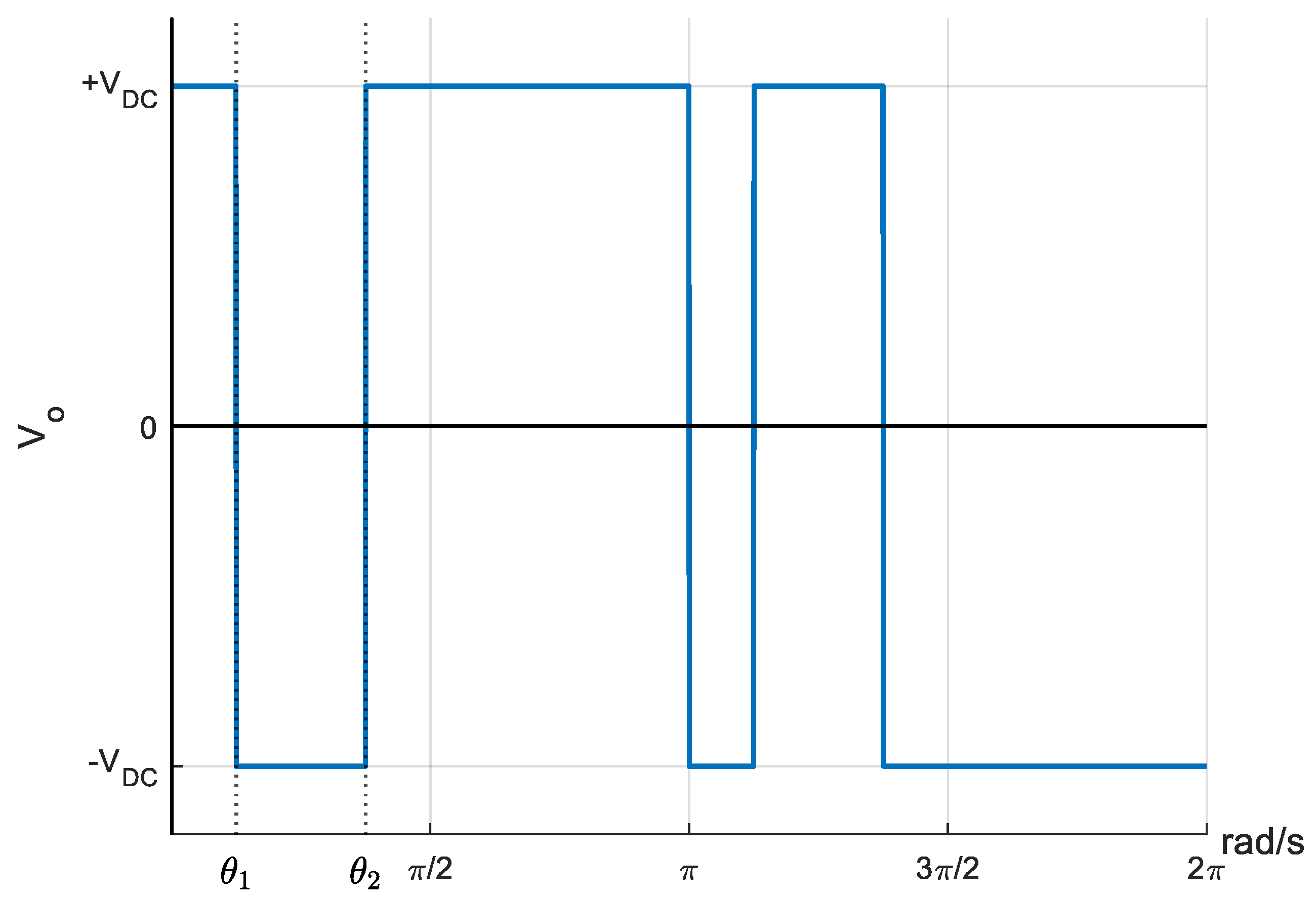
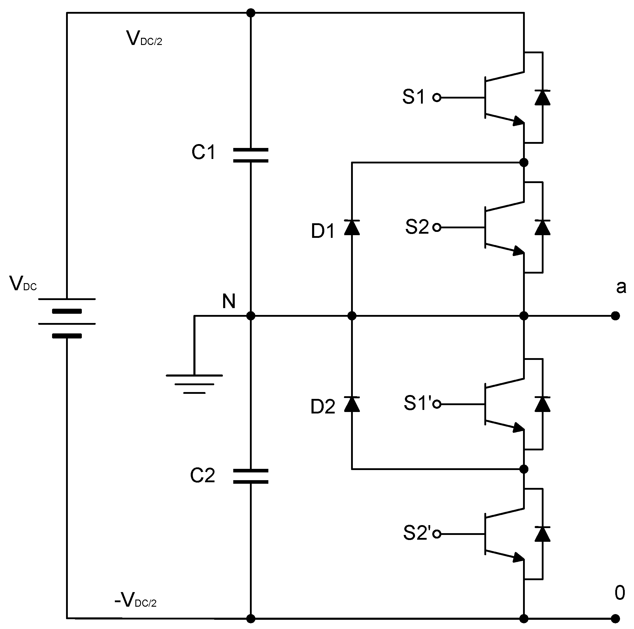
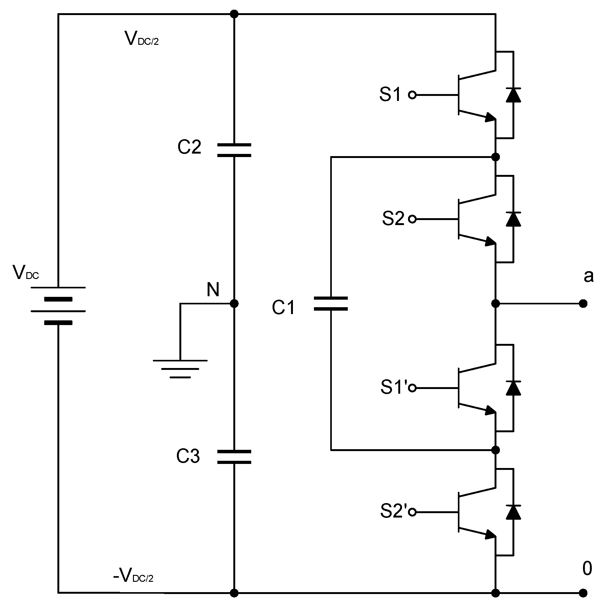
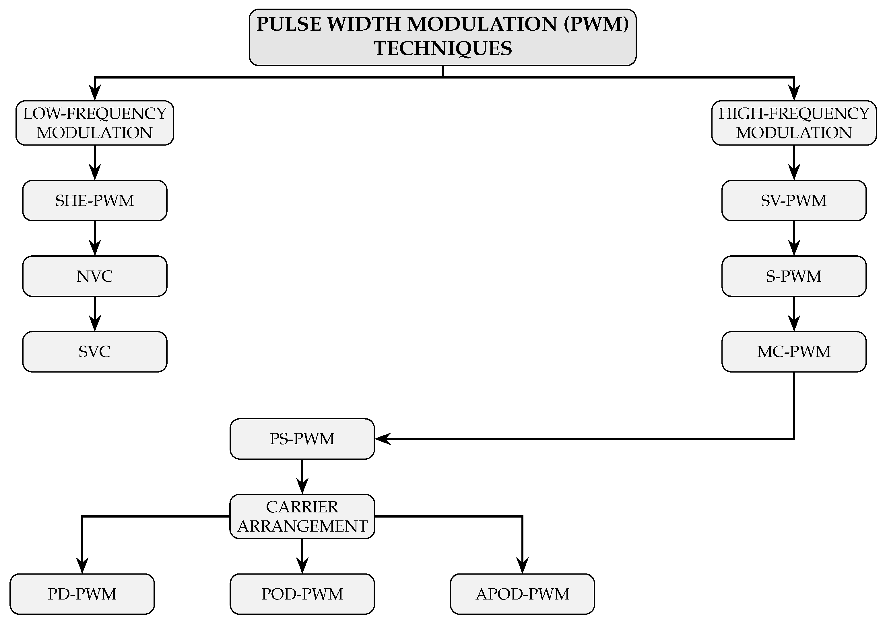
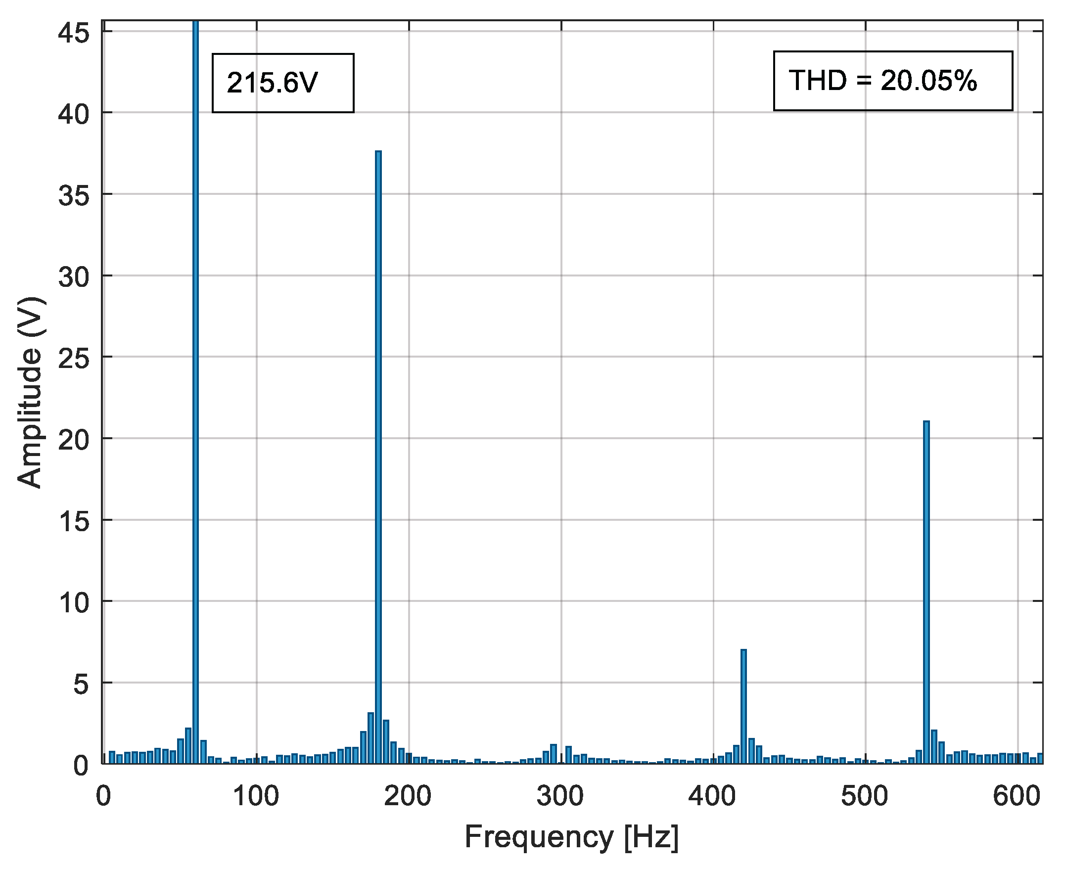
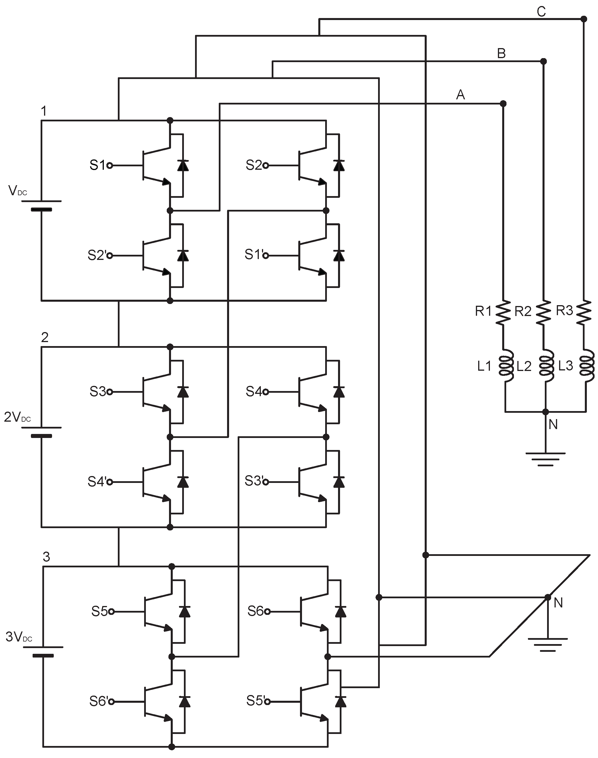
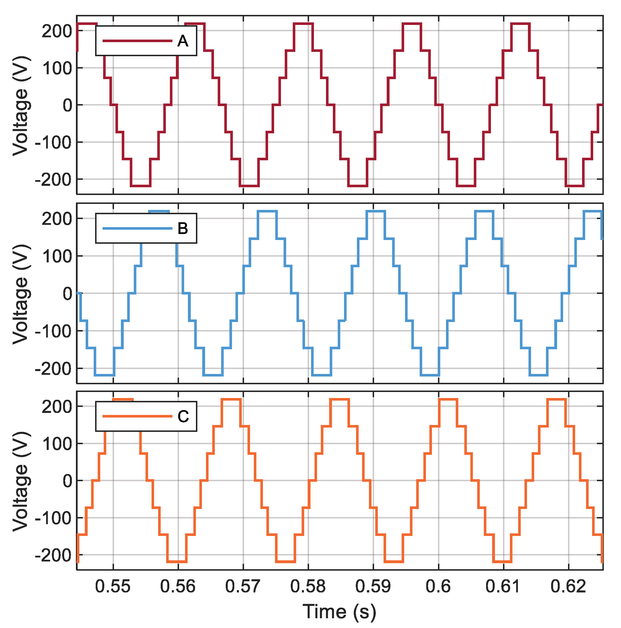
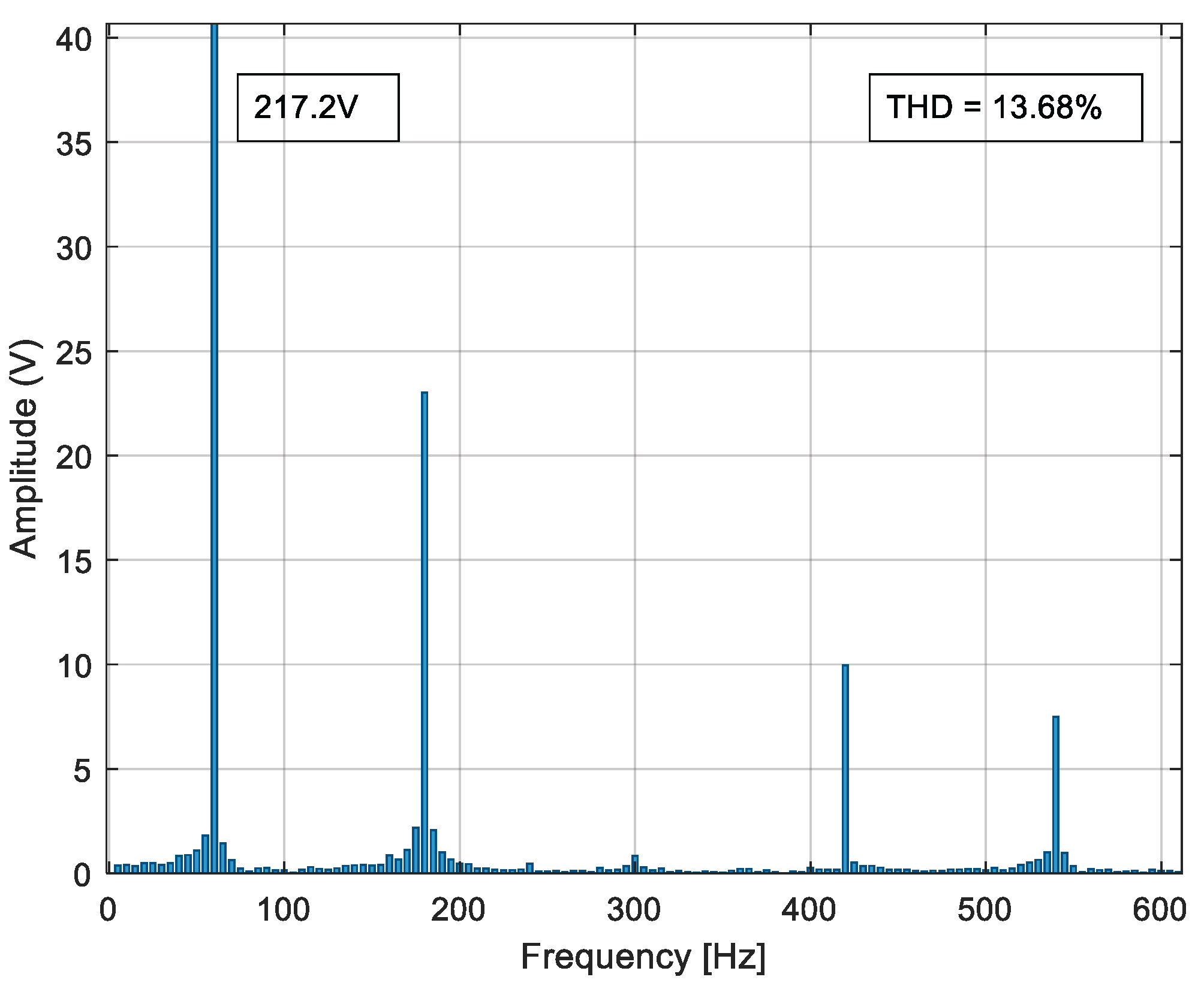
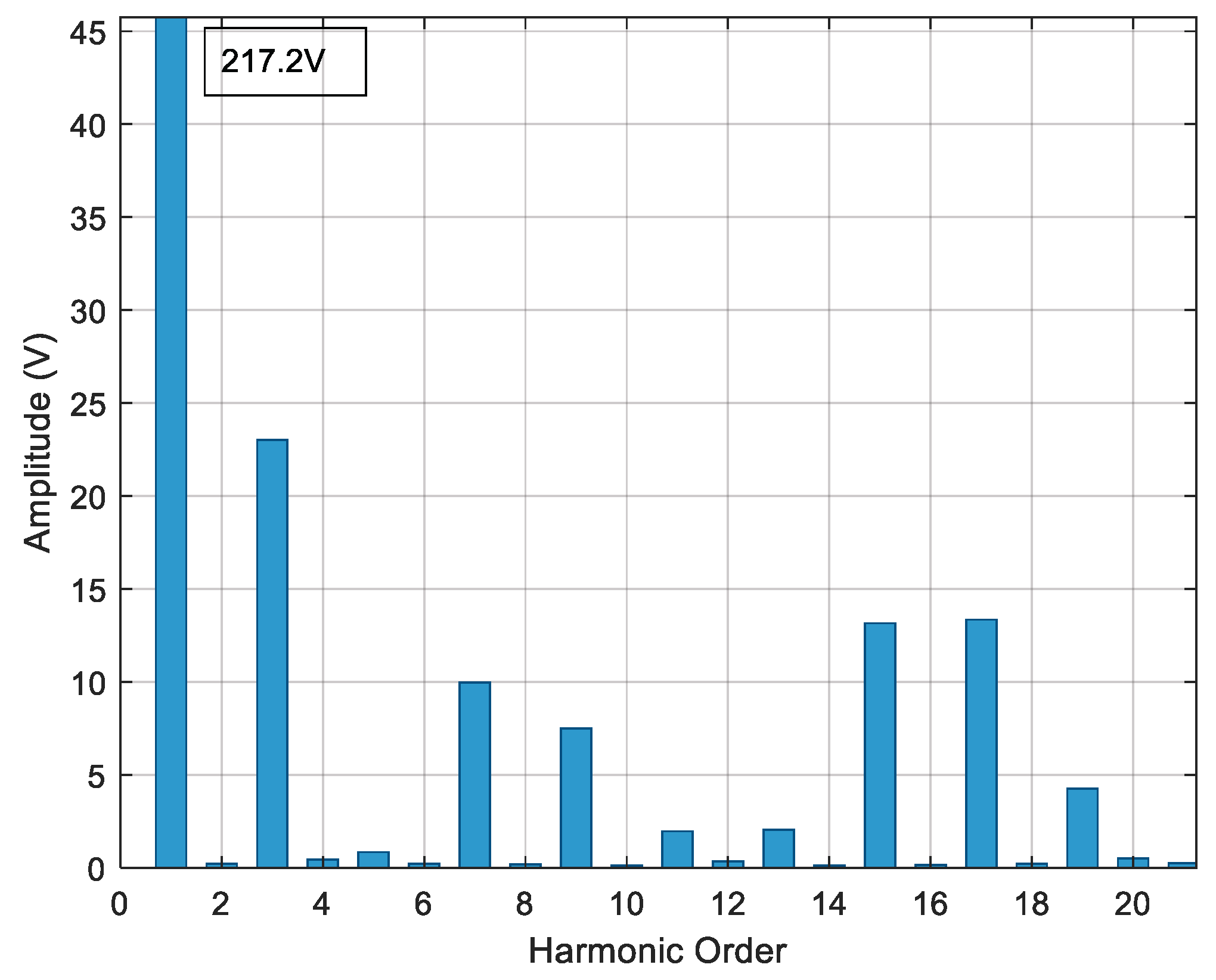
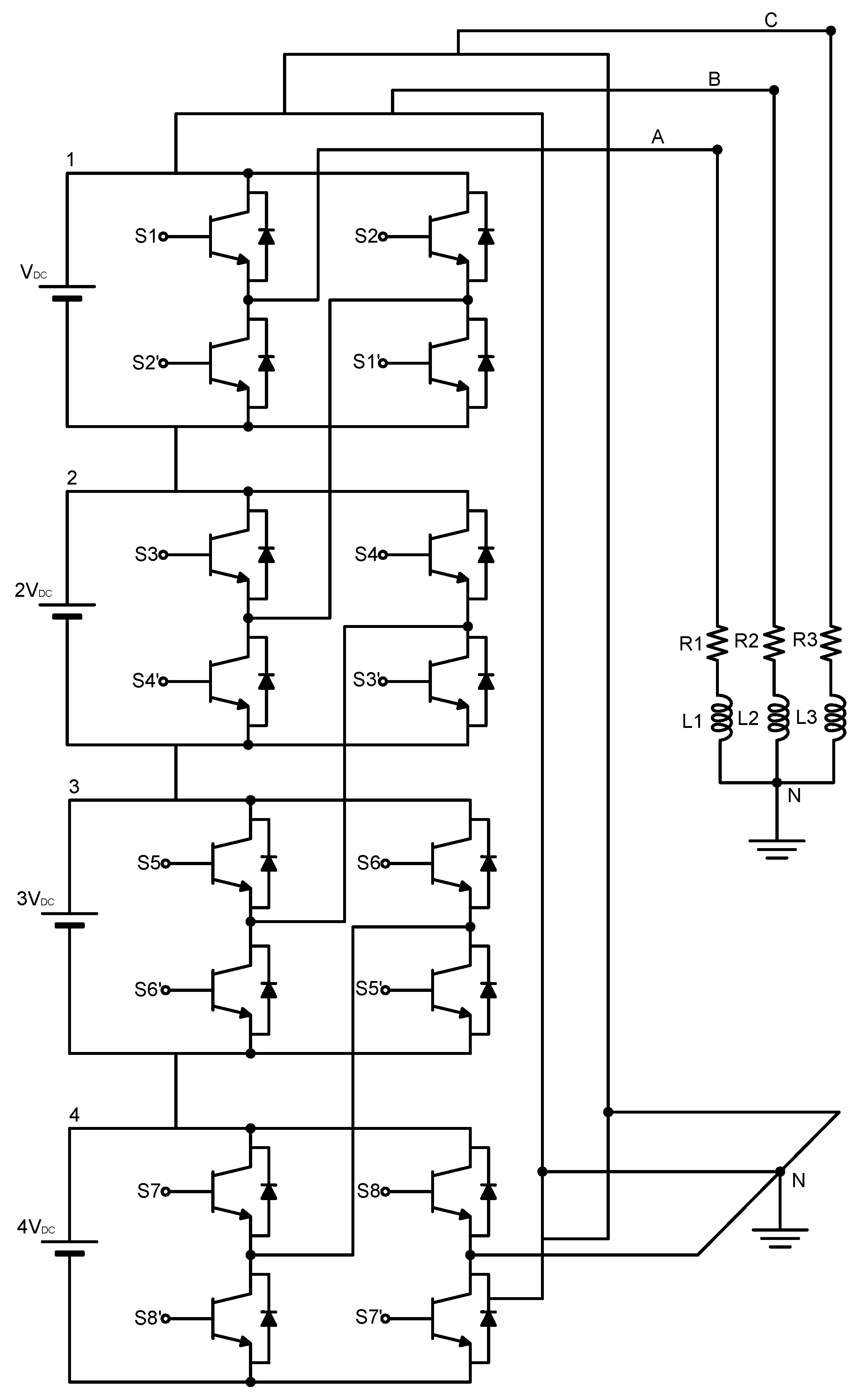
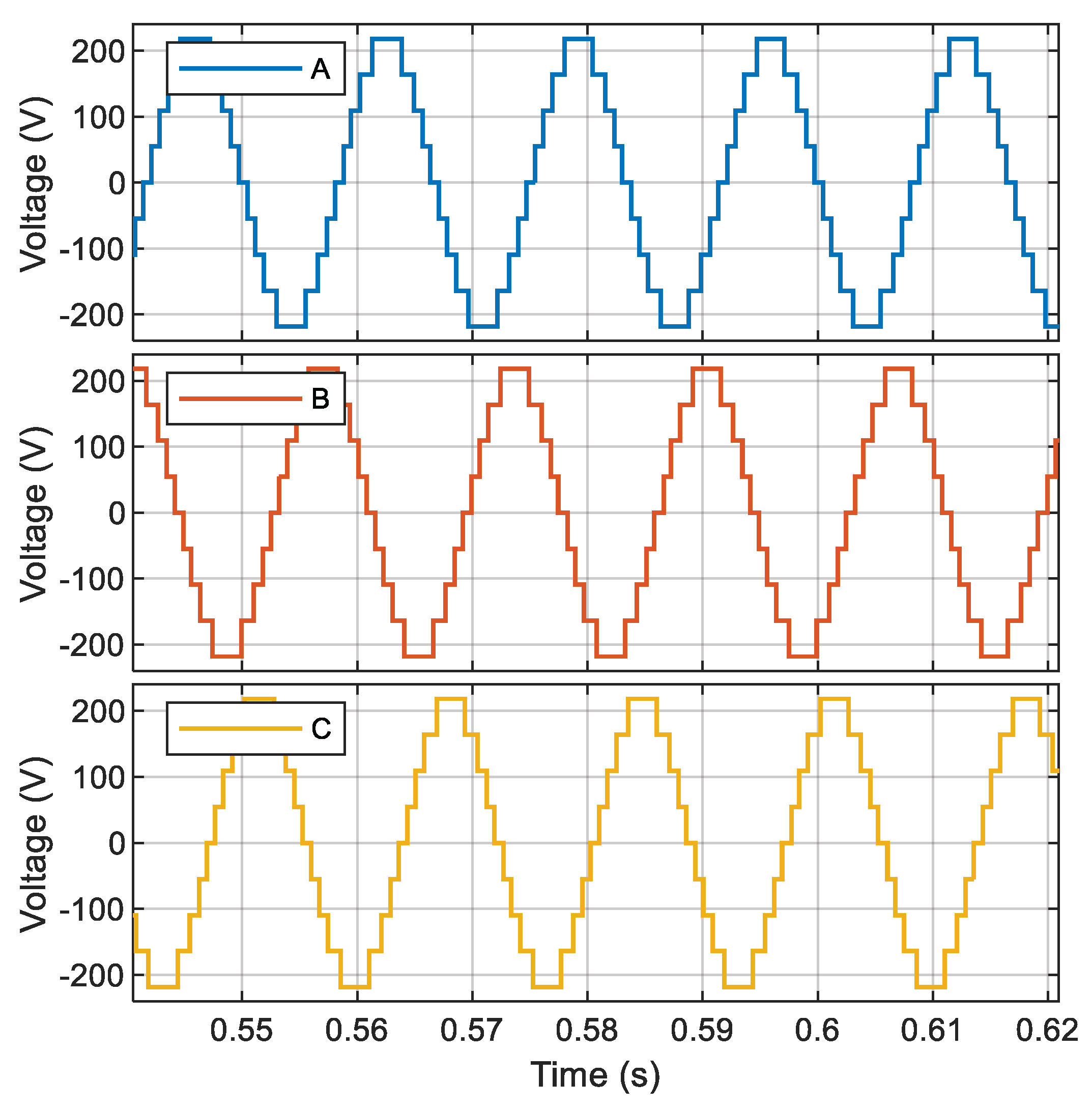
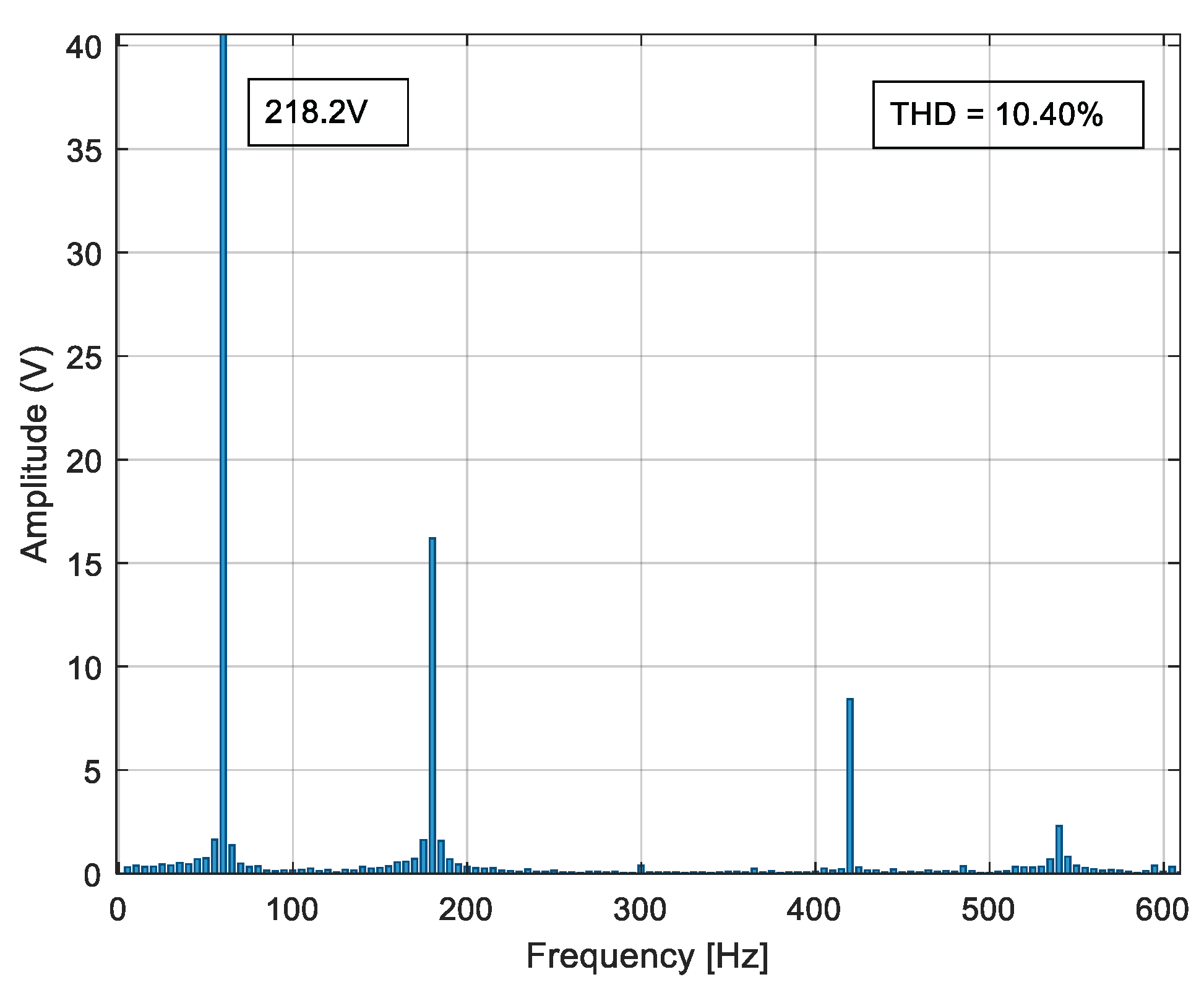
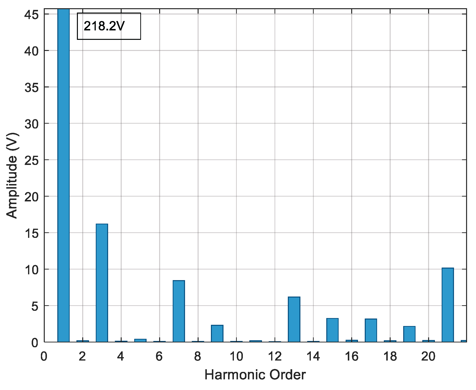
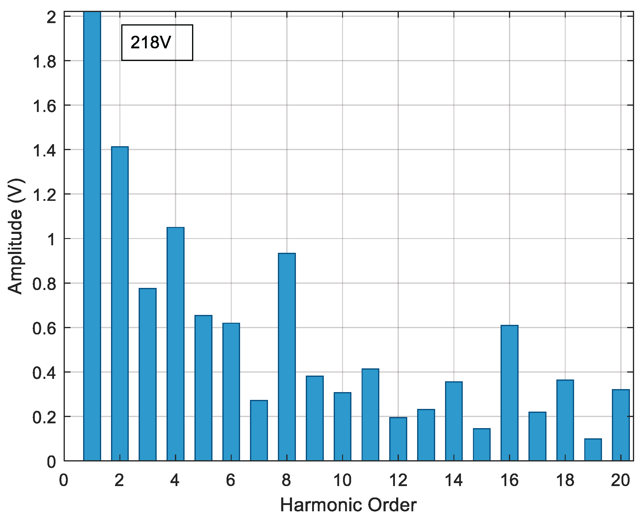
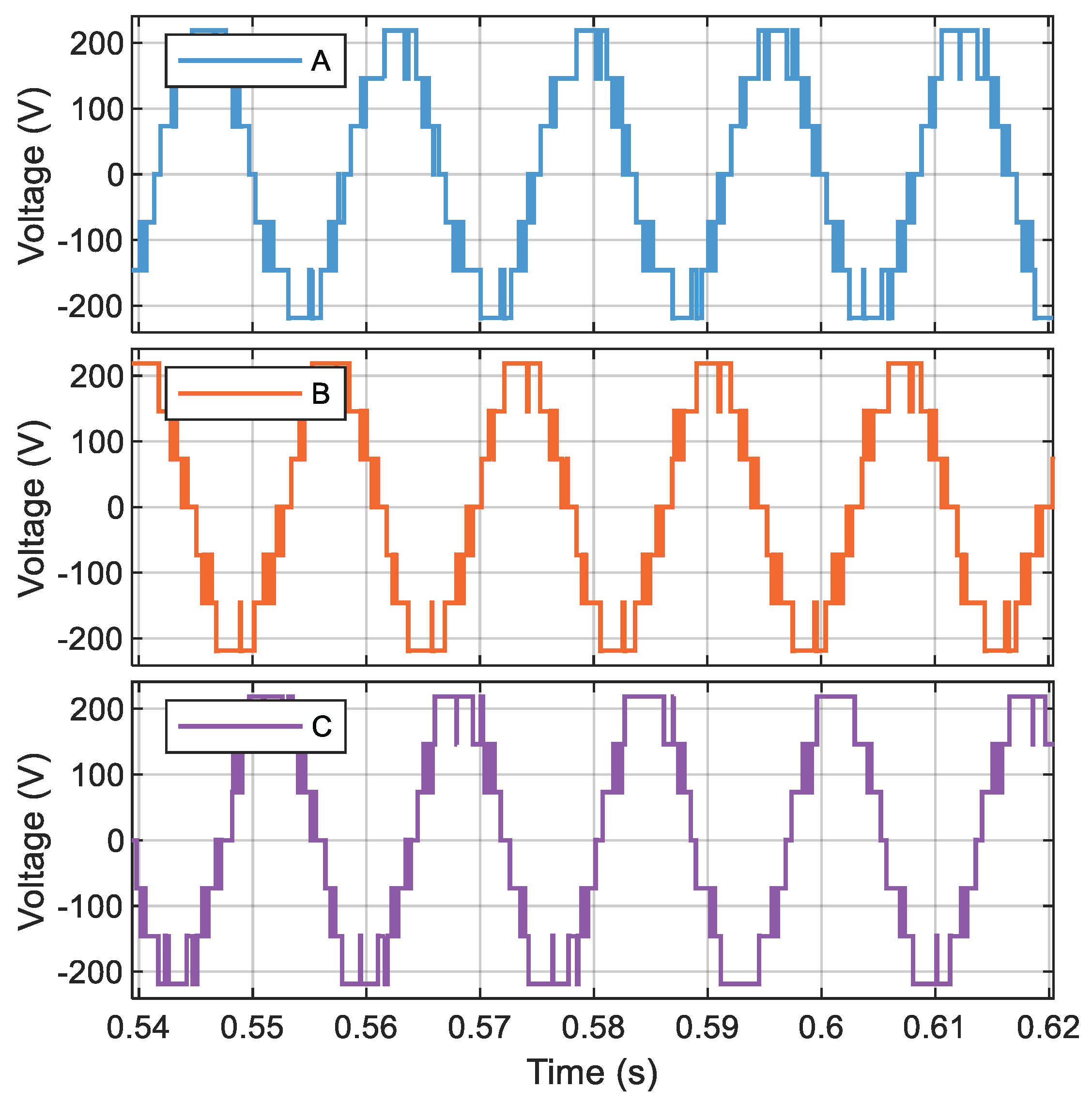
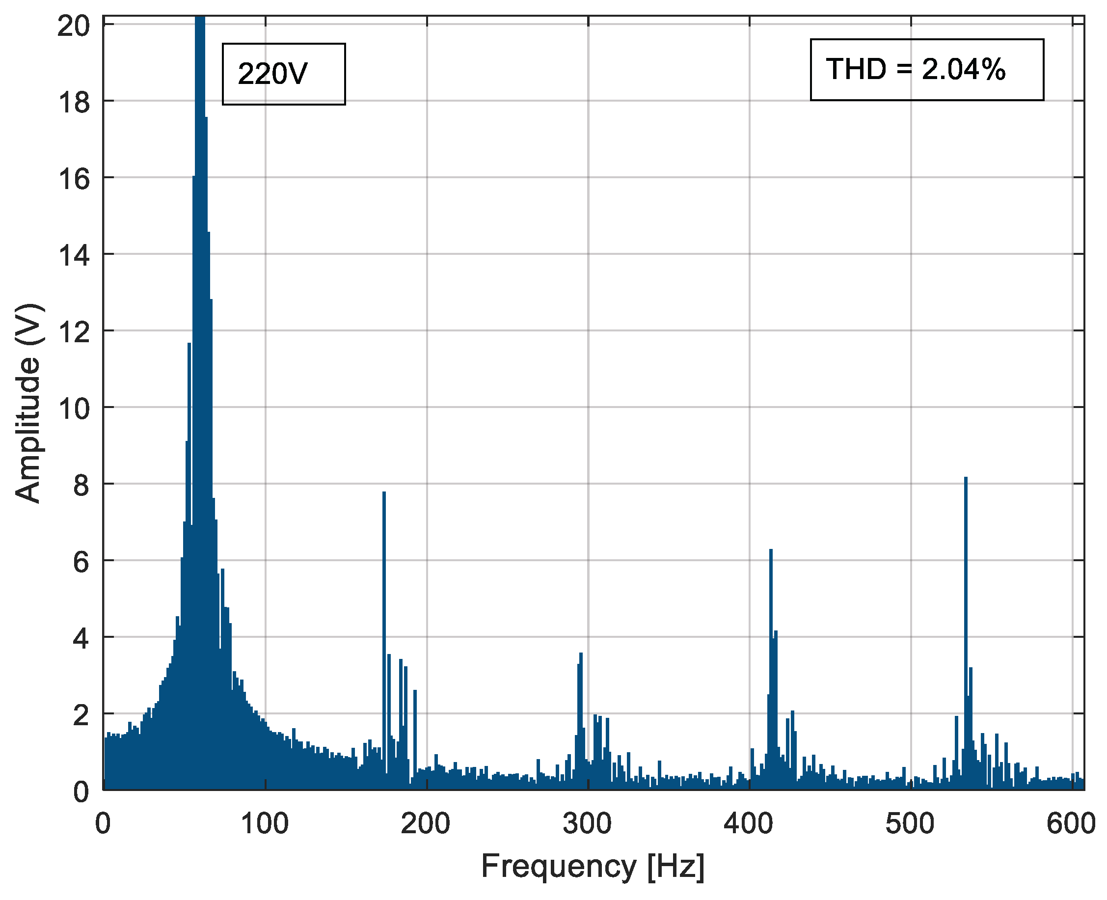
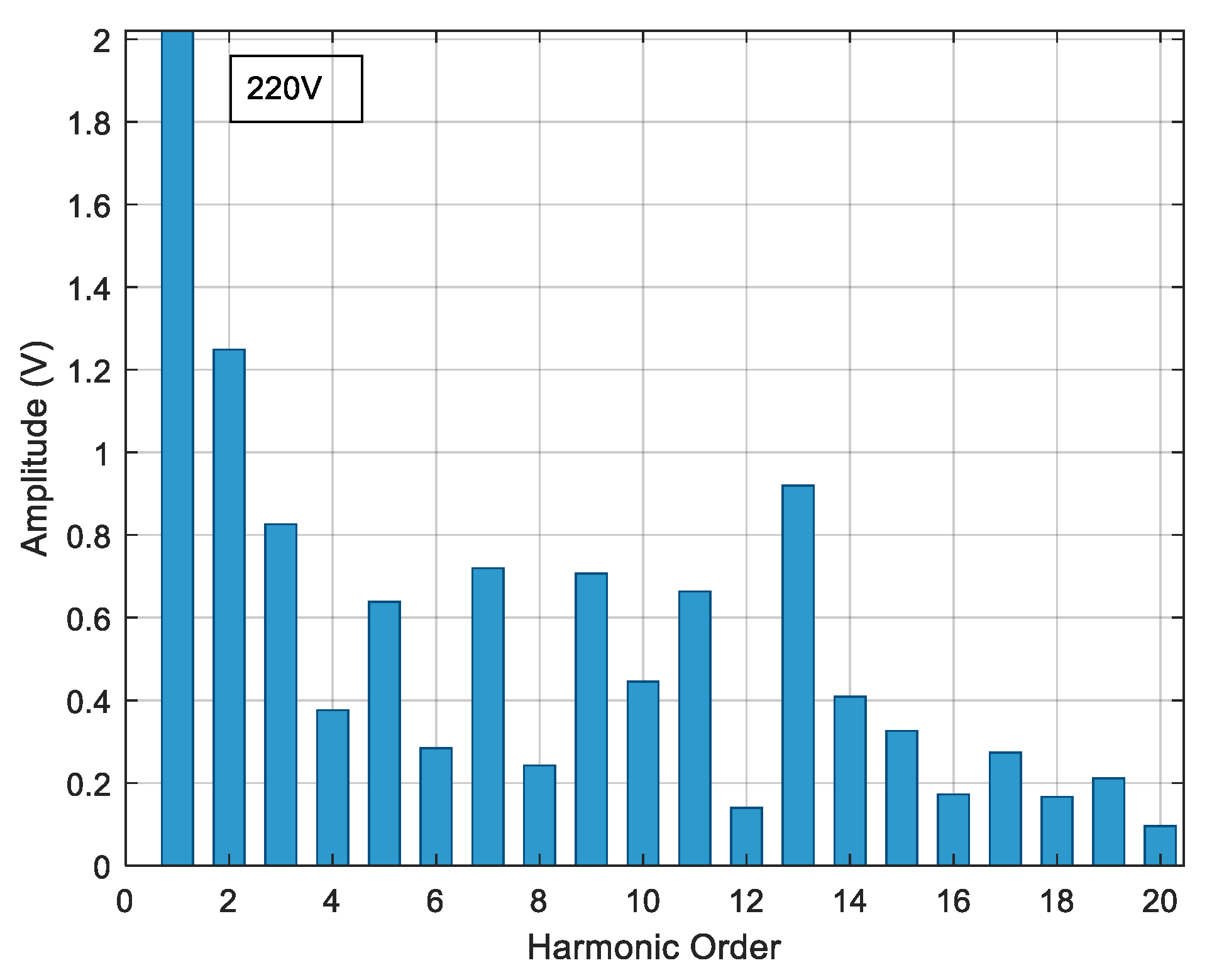
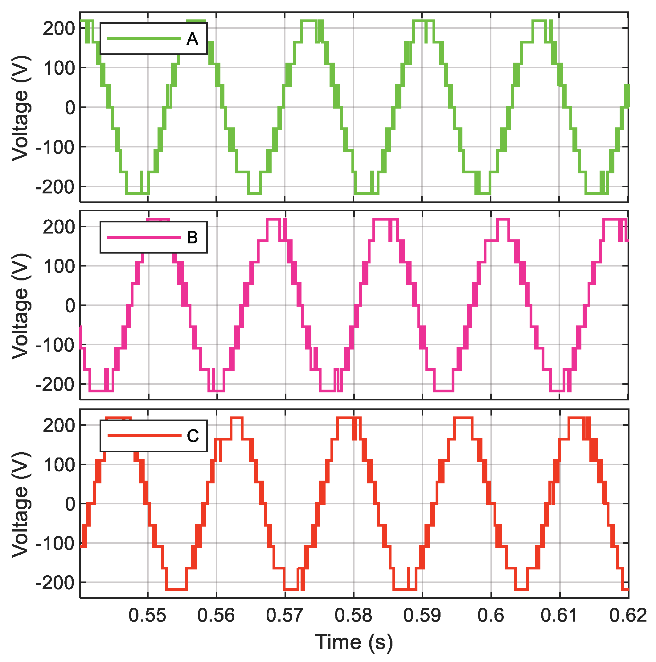
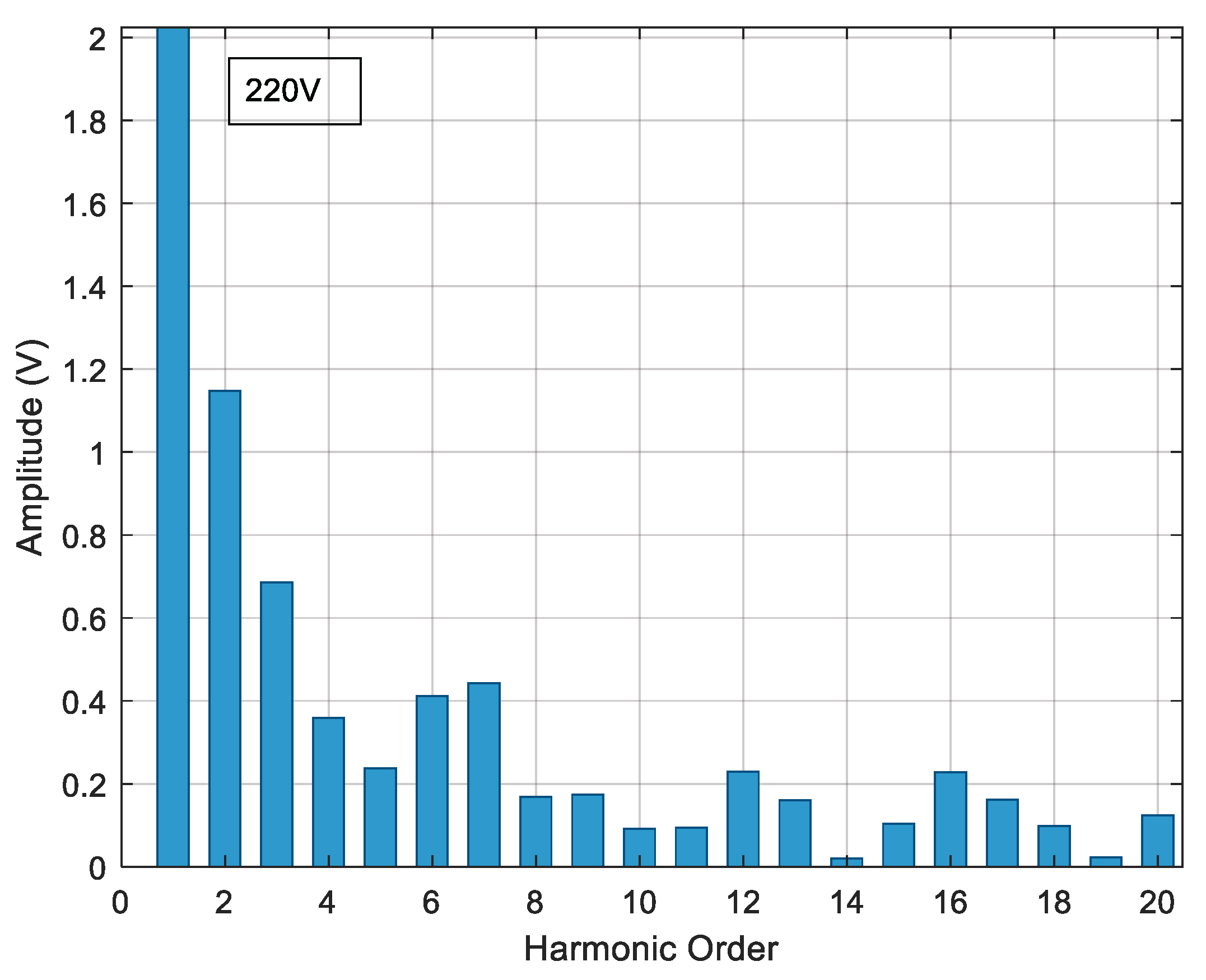
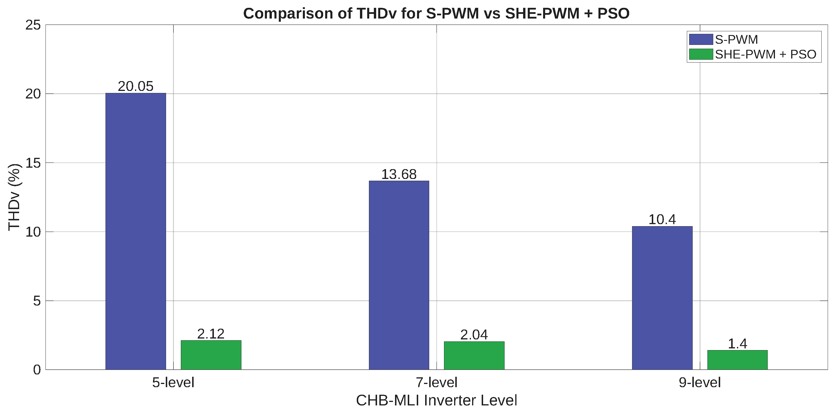
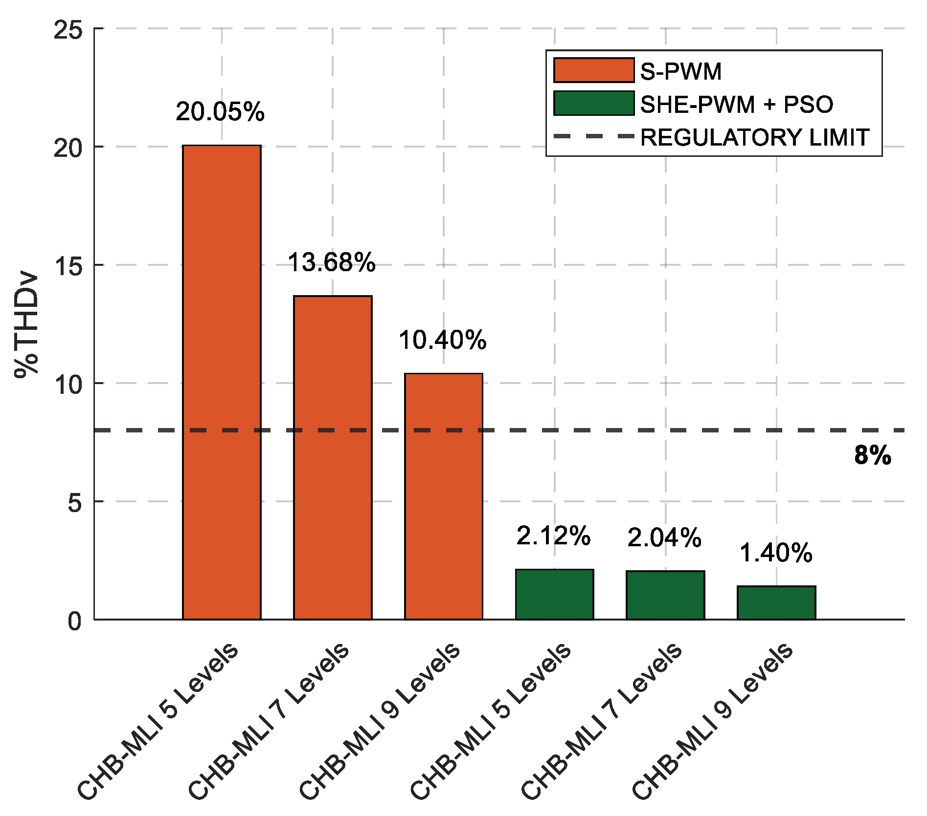
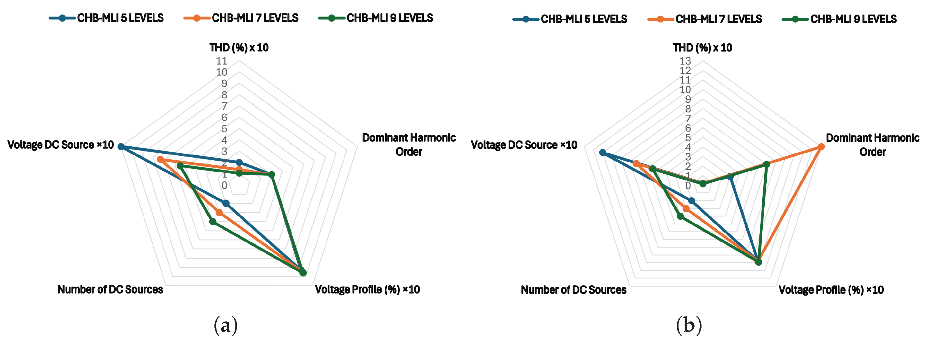
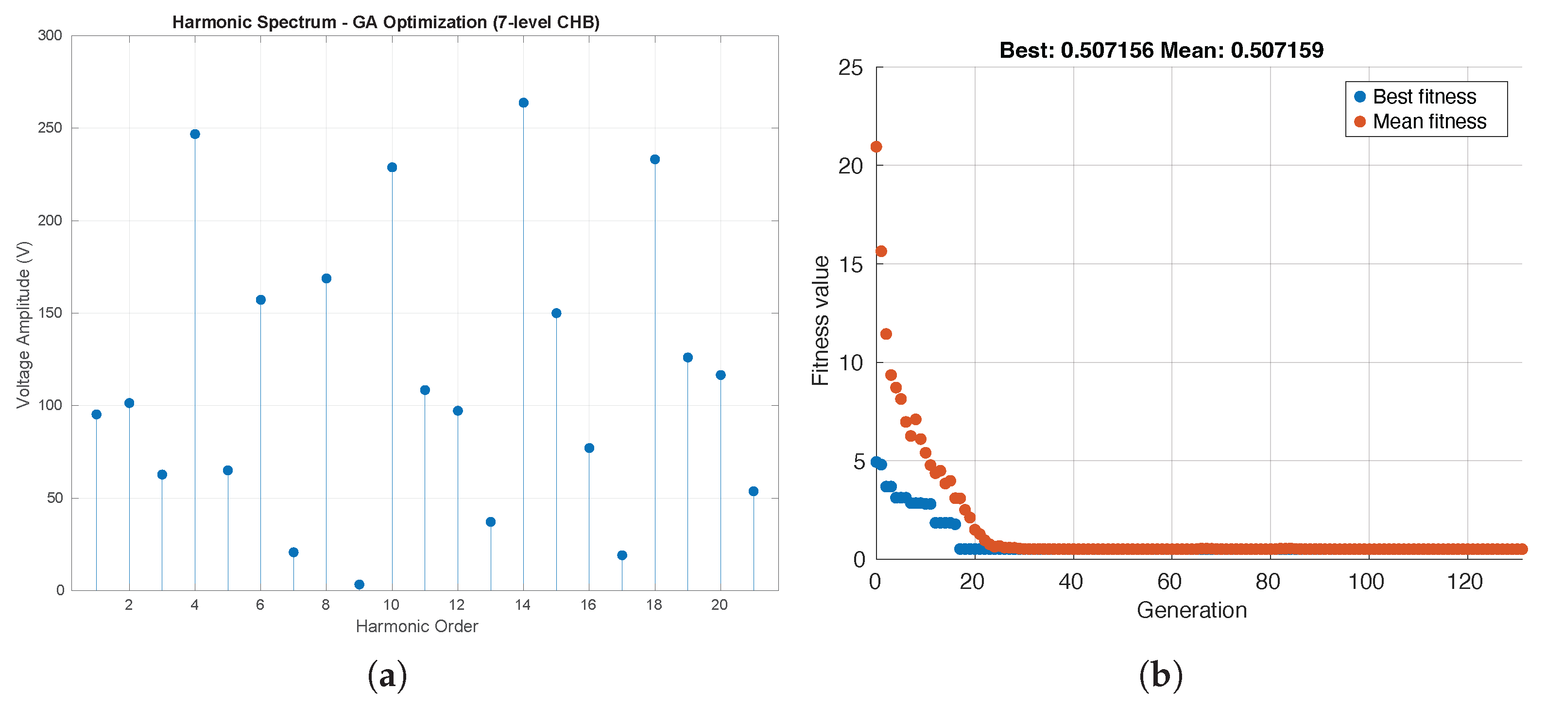
The process described at the beginning of this chapter is developed for each proposed case study to reduce the voltage THDv percentage by reducing the most prevalent harmonics in each inverter model.

3.3.1. Formulation of the Modulation Technique

The SHE-PWM modulation technique is developed from a single-phase perspective. By working better with each voltage signal generated by the inverter, it facilitates the determination of firing angles. The nonlinear equations for these are appropriately formulated so that, to achieve modulation of the remaining phases, only 120 degrees are shifted from the results obtained in the first phase. The harmonics of interest to suppress with this technique are the lower-order harmonics (3rd, 5th, 7th, 9th, 11th, etc.), especially the odd ones, which significantly increase the THDv percentage in the output voltage signal. Harmonics beyond the 15th order were excluded from the optimization since their amplitudes are negligible and do not significantly contribute to voltage THDv. Moreover, high-order harmonics are easier to attenuate using passive filters if necessary, and their impact on power quality is minimal compared to lower-order harmonics [5,6]. These harmonics cause power quality issues, including voltage fluctuations, interference with sensors and control systems, and equipment overheating. They have a direct impact on electrical machines such as motors and generators, causing pulsating torque that translates into mechanical vibrations and, consequently, a reduction in their useful life. It is also related to losses and problems in electrical equipment, such as Joule losses, hysteresis losses, eddy currents, and leakage currents, which cause undesirable and often premature deterioration of the equipment. Each CHB-MLI inverter structure presents a set of parameters with which the SHE-PWM with Fourier is formulated, such as the number of allowed angles, the harmonics of interest to be suppressed, the modulation index for the fundamental component, and the operating frequency. The number of firing angles that define the stepped waveform for a quarter-cycle of the voltage signal is related to the number of levels of each inverter, as shown in Equation (12). Therefore, this is considered a restriction on the number of angles that can be obtained for each case study. The Fourier series expression is formulated based on Equation (13), with the difference that the global amplitude factor for the signal magnitude is excluded, as the elimination of harmonics depends solely on the sum of cosines, representing the variable part of the signal controlled by the firing angles. Therefore, the system of nonlinear Equation (16) is proposed for each case study. In formulating this modulation technique, the aim is to preserve the amplitude of the fundamental signal, bringing it close to the desired value of 220 V. For this reason, the modulation factor m used in the formulation of the system of equations and in the objective function has a value equal to 1 to ensure that the fundamental component is not affected.

3.3.2. Five-Level CHB-MLI Inverter

The following parameters are proposed for this inverter structure:

• $N=2$ switching angles, ${\theta }_1$ and ${\theta }_2$;
• $f=60$ Hz;
• $h=\{3,7\}$ (harmonics to eliminate);
• $m=1$.

Fourier Series Expression:

$$V_{(3,7)}=\sum _{i=1}^{2}cos\left(h{\theta }_i\right)$$

(19)

Nonlinear Equation System:

$$\begin{array}{cc}\hfill 1& =cos\left({\theta }_1\right)+cos\left({\theta }_2\right)\hfill \\ \hfill 0& =cos\left(3{\theta }_1\right)+cos\left(3{\theta }_2\right)\hfill \\ \hfill 0& =cos\left(7{\theta }_1\right)+cos\left(7{\theta }_2\right)\hfill \end{array}$$

(20)

Objective Function:

$$f({\theta }_1,{\theta }_2)=\sum _{h\in \{3,7\}}{\left(\sum _{i=1}^{2}cos\left(h{\theta }_i\right)\right)}^2+\lambda {\left(\sum _{i=1}^{2}cos\left({\theta }_i\right)-m\right)}^2$$

(21)

The first term minimizes the selected harmonics, while the second ensures that the fundamental component is preserved, controlled by m and $\lambda$.

3.3.3. Seven-Level CHB-MLI Inverter

Parameters for this inverter structure:

• $N=3$ switching angles, ${\theta }_1$, ${\theta }_2$, ${\theta }_3$;
• $f=60$ Hz;
• $h=\{3,7,9\}$;
• $m=1$.

As detailed in Figure 17, the 3rd, 7th, and 9th order harmonics are the most prominent, with the highest amplitudes within the spectrum. They are the most dominant in total strength. The 11th-order harmonic does exist; however, its contribution is relatively small. Given that the SHE-PWM control method for this inverter permits only three switching angles, it becomes necessary to focus on the dominant harmonic that is the most impactful for reducing harmonic distortion (THDv).

Fourier Series Expression:

$$V_{(3,7,9)}=\sum _{i=1}^{3}cos\left(h{\theta }_i\right)$$

(22)

Nonlinear Equation System:

$$\begin{array}{cc}\hfill 1& =cos\left({\theta }_1\right)+cos\left({\theta }_2\right)+cos\left({\theta }_3\right)\hfill \\ \hfill 0& =cos\left(3{\theta }_1\right)+cos\left(3{\theta }_2\right)+cos\left(3{\theta }_3\right)\hfill \\ \hfill 0& =cos\left(7{\theta }_1\right)+cos\left(7{\theta }_2\right)+cos\left(7{\theta }_3\right)\hfill \\ \hfill 0& =cos\left(9{\theta }_1\right)+cos\left(9{\theta }_2\right)+cos\left(9{\theta }_3\right)\hfill \end{array}$$

(23)

Objective Function:

$$f({\theta }_1,{\theta }_2,{\theta }_3)=\sum _{h\in \{3,7,9\}}{\left(\sum _{i=1}^{3}cos\left(h{\theta }_i\right)\right)}^2+\lambda {\left(\sum _{i=1}^{3}cos\left({\theta }_i\right)-m\right)}^2$$

(24)

3.3.4. Nine-Level CHB-MLI Inverter

Parameters for this inverter structure:

• $N=4$ switching angles, ${\theta }_1$, ${\theta }_2$, ${\theta }_3$, ${\theta }_4$;
• $f=60$ Hz;
• $h=\{3,7,9,13\}$;
• $m=1$.

Fourier Series Expression:

$$V_{(3,7,9,13)}=\sum _{i=1}^{4}cos\left(h{\theta }_i\right)$$

(25)

Nonlinear Equation System:

$$\begin{array}{cc}\hfill 1& =cos\left({\theta }_1\right)+cos\left({\theta }_2\right)+cos\left({\theta }_3\right)+cos\left({\theta }_4\right)\hfill \\ \hfill 0& =cos\left(3{\theta }_1\right)+cos\left(3{\theta }_2\right)+cos\left(3{\theta }_3\right)+cos\left(3{\theta }_4\right)\hfill \\ \hfill 0& =cos\left(7{\theta }_1\right)+cos\left(7{\theta }_2\right)+cos\left(7{\theta }_3\right)+cos\left(7{\theta }_4\right)\hfill \\ \hfill 0& =cos\left(9{\theta }_1\right)+cos\left(9{\theta }_2\right)+cos\left(9{\theta }_3\right)+cos\left(9{\theta }_4\right)\hfill \\ \hfill 0& =cos\left(13{\theta }_1\right)+cos\left(13{\theta }_2\right)+cos\left(13{\theta }_3\right)+cos\left(13{\theta }_4\right)\hfill \end{array}$$

(26)

Objective Function:

$$f({\theta }_1,{\theta }_2,{\theta }_3,{\theta }_4)=\sum _{h\in \{3,7,9,13\}}{\left(\sum _{i=1}^{4}cos\left(h{\theta }_i\right)\right)}^2+\lambda {\left(\sum _{i=1}^{4}cos\left({\theta }_i\right)-m\right)}^2$$

(27)

3.3.5. Description of the Optimization Algorithm

The proposed Algorithms 1 and 2 aim to determine the optimal switching angles for a SHE-PWM signal using Particle Swarm Optimization (PSO).

Algorithm 1 SHE-PWM Optimization Using PSO.

1: Input: $n\_angles$, $harmonics\_to\_eliminate$, $M_{target}$   2: PSO Parameters: N, $iter$, w, $c_1$, $c_2$, $lb$, $ub$   3: Initialization:   4:    Set $v=0$ (initial velocity)   5:    Set $pbest=x$   6:    Set $gbest=x[1,:]$   7:    Initialize $f\_pbest=\infty$, $f\_gbest=\infty$   8: Initial Evaluation:   9: for  $i=1$  to  N  do 10:     $f\_pbest\left[i\right]\leftarrow CALCULATE\_FITNESS(x[i,:],harmonics\_to\_eliminate,M_{target})$ 11:     if $f\_pbest\left[i\right]<f\_gbest$ then 12:         $f\_gbest\leftarrow f\_pbest\left[i\right]$ 13:         $gbest\leftarrow x[i,:]$ 14:     end if 15: end for 16: Iterations: 17: for  $t=1$  to  $iter$  do 18:     for $i=1$ to N do 19:         Update velocity: $$v[i,:]\leftarrow w·v[i,:]+c_1·\mathrm{rand}\left(\right)·(pbest[i,:]-x[i,:])+c_2·\mathrm{rand}\left(\right)·(gbest-x[i,:])$$ 20:         Update position: $$x[i,:]\leftarrow x[i,:]+v[i,:]$$ 21:         Limit $x[i,:]$ to $[lb,ub]$ 22:         $f\leftarrow CALCULATE\_FITNESS(x[i,:],harmonics\_to\_eliminate,M_{target})$ 23:         if $f<f\_pbest\left[i\right]$ then 24:            $pbest[i,:]\leftarrow x[i,:]$ 25:            $f\_pbest\left[i\right]\leftarrow f$ 26:            if $f<f\_gbest$ then 27:                $gbest\leftarrow x[i,:]$ 28:                $f\_gbest\leftarrow f$ 29:            end if 30:         end if 31:     end for 32:     $w\leftarrow w·0.99$ 33:     if $w<0.48$ then 34:         $w\leftarrow 0.48$ 35:     end if 36: end for 37: Output: 38: Convert $gbest$ to degrees, sort, and print 39: $gbest\leftarrow$ optimal solution 40: Calculate and print Fourier components: $$f\left(h\right)=\sum _{i=1}^N{(-1)}^{i-1}cos(h·gbest\left[i\right])$$

Algorithm 2 Objective Function calcuFitness.

1: Input: $\theta$, $harmonics\_to\_eliminate$, $M_{target}$, $\lambda$   2: Calculate fundamental error: $$error\_fund={\left[\left(\sum _{i=1}^N{(-1)}^{i-1}cos\left({\theta }_i\right)\right)-M_{target}\right]}^2$$   3: Initialize $sum\_harm=0$   4: for each  h  in  $harmonics\_to\_eliminate$  do   5:     $sum={\sum }_{i=1}^N{(-1)}^{i-1}cos(h·{\theta }_i)$   6:     $sum\_harm\leftarrow sum\_harm+su{m}^2$   7: end for   8: Compute the objective function: $$f=sum\_harm+\lambda ·error\_fund$$ (28)   9: Return:  f 10: End

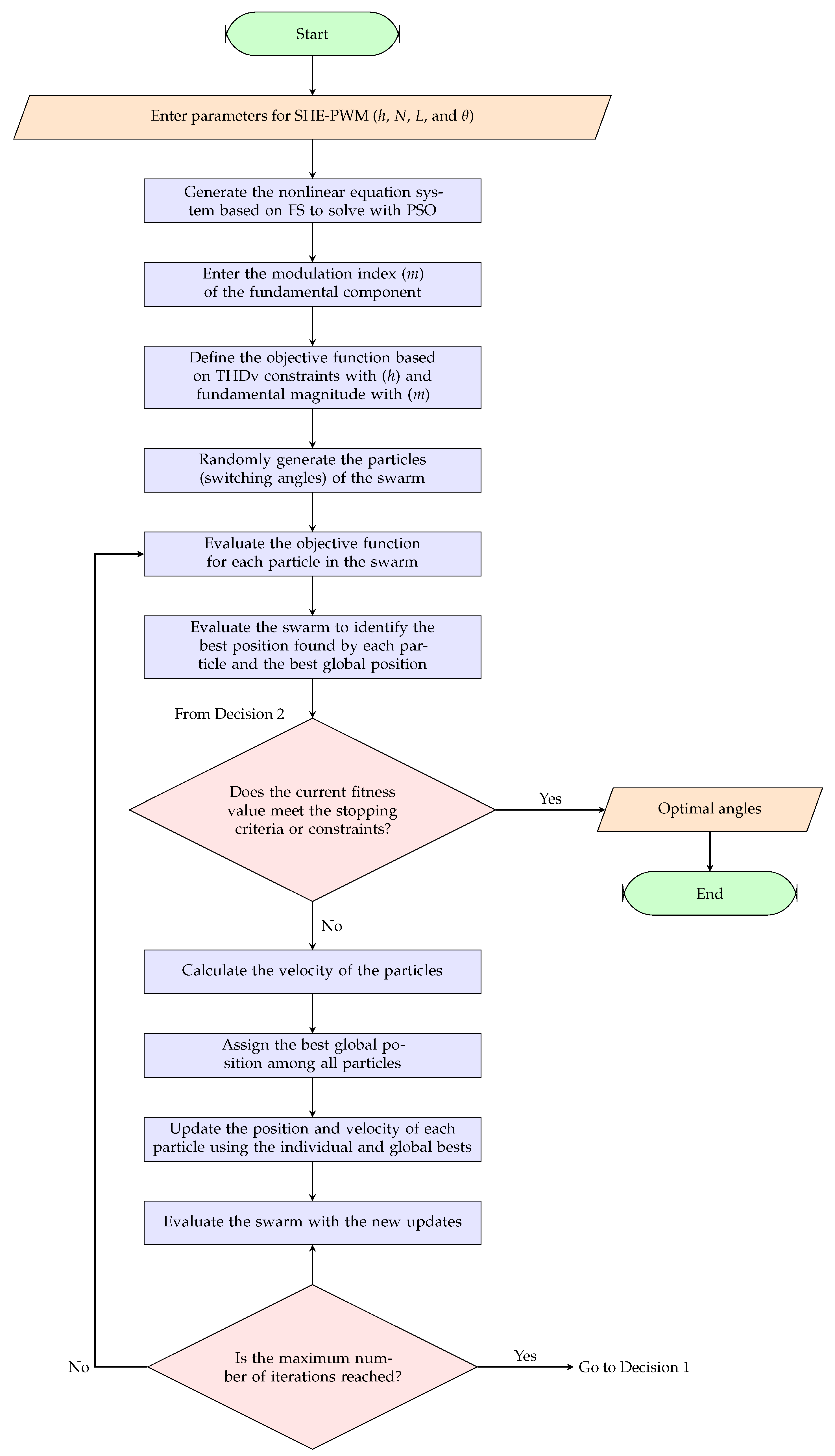
The developed objective function verifies the reduction of unwanted harmonics and how close the value of the fundamental component is to the target value defined with the modulation m and the weighting factor $\lambda$. The algorithm is described in the following steps:

• Parameter initialization: Input and configuration values for the PSO are defined, such as the number of firing angles ($n_{ang}$), harmonics to be eliminated ($ar{m}_{eli}$), the value of the fundamental component ($M_{obj}$), the number of particles (N), the number of iterations (iter), the inertial weight (w), the cognitive and social attraction coefficients ($c_1$ and $c_2$), and the lower and upper bounds for the angles in the search space (lb and ub).
• Generation of the initial population: Positions x are randomly initialized within the search space defined by [lb − ub]. The velocities v are initialized to zero. The best individual position (pbst) is set as the initial position, and a seed is selected for the best global position (gbst). The fitness values ($f_{pbst}$ and $f_{gbst}$) are initialized to infinity.
• Initial population evaluation: The objective function for each particle is evaluated using calcuFitness, which considers the fundamental component error and the squared error of the harmonics of interest. The pbst and gbst values are updated based on the best value obtained.
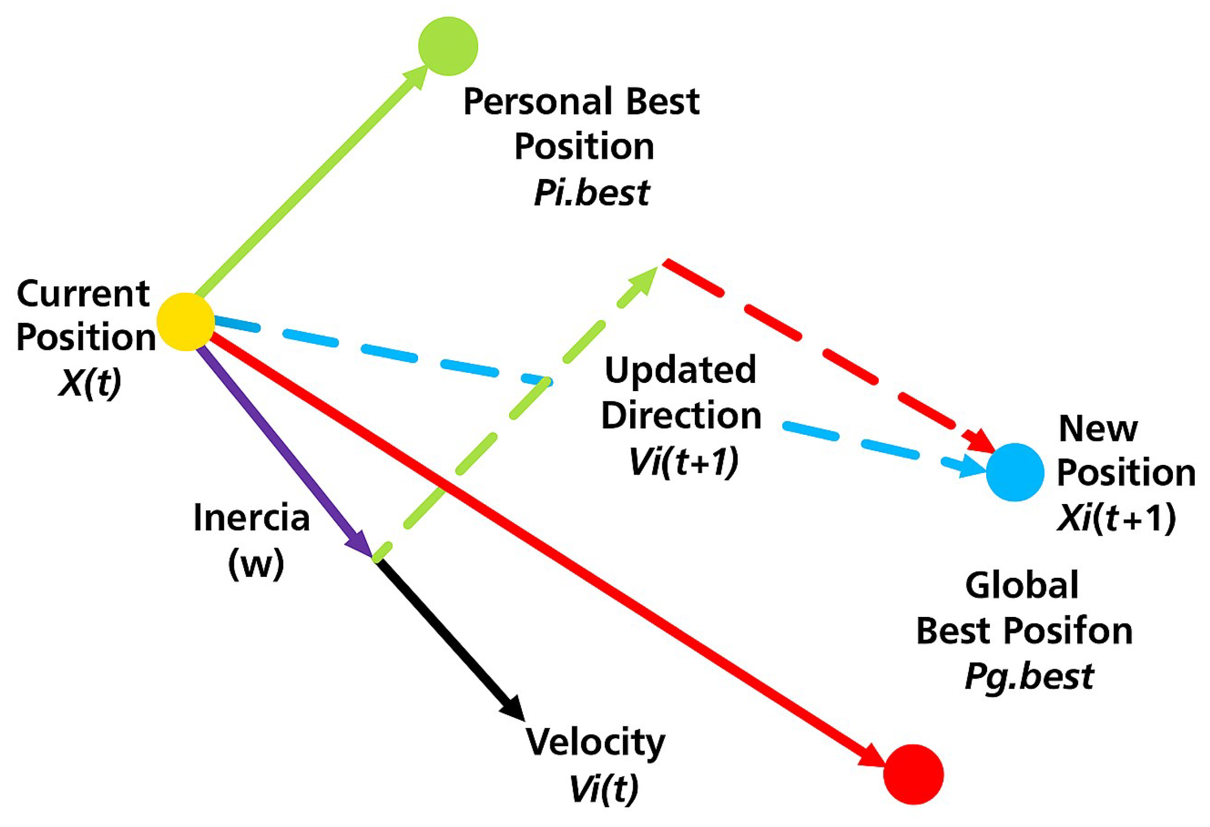
• PSO iterations: Each particle is updated in both velocity and position using Equations (7) and (9), respectively. Positions are limited within the valid angle range [lb ub]. The objective function is re-evaluated, and if the fitness values improve ($f_{pbst}$ and $f_{gbst}$), they are updated with their corresponding positions (pbst and gbst). A progressive inertial weight-damping strategy is applied to refine solutions close to the optimum.
• Obtaining results: At the end of the iterations, the best global solution (gbst) is selected, which represents the optimal set of firing angles. These angles are converted to degrees and sorted in ascending order. Finally, the harmonic components are calculated using the Fourier Series with the optimal angles obtained.

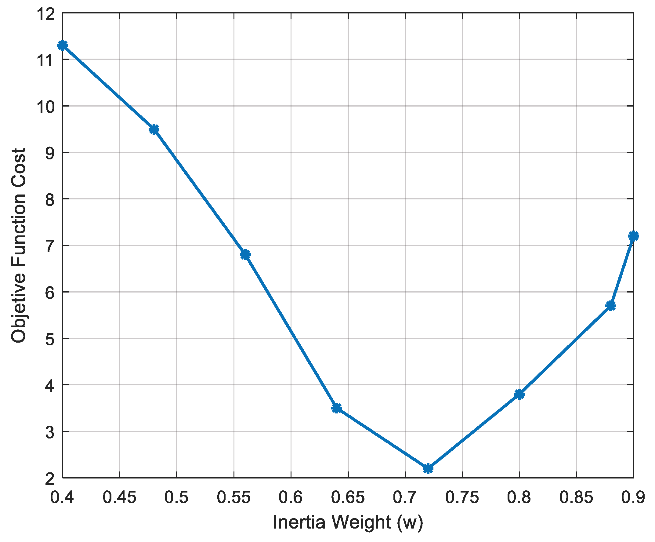
Configuration of PSO parameters: To configure the PSO parameters, a sensitivity analysis is performed to justify the numerical values of the parameters w, $c_1$, $c_2$, and $\lambda$. The goal is to ensure that the selected value corresponds to the lowest cost of the objective function, as this represents an efficient and optimal solution. However, a high cost of the objective function indicates a poor or suboptimal solution. This demonstrates the limitations of the algorithm in the face of parameter variation, ensuring replicability for future case studies. Inertia weight (w): Regulates the balance between the exploration and exploitation mechanisms in the search space. It is related to the previous velocity of the particle for the current motion, thus determining the degree of persistence in its trajectory. Typically, a range of values is used between [0.4–0.9]. Eight random values for w are evaluated within the optimal range between [0.4–0.9], with fixed values of 1.5 for $c_1$ and $c_2$, and $\lambda$ is not considered, with the aim of achieving the lowest cost for the objective function.

Values to be evaluated: [0.4, 0.48, 0.56, 0.64, 0.72, 0.80, 0.88, 0.9]

Figure 22 shows how the cost of the objective function gradually decreases as it approaches a value of w equal to 0.65, reaching its minimum at w equal to 0.72, and then increasing its cost again as the value of w rises until it reaches 0.9.

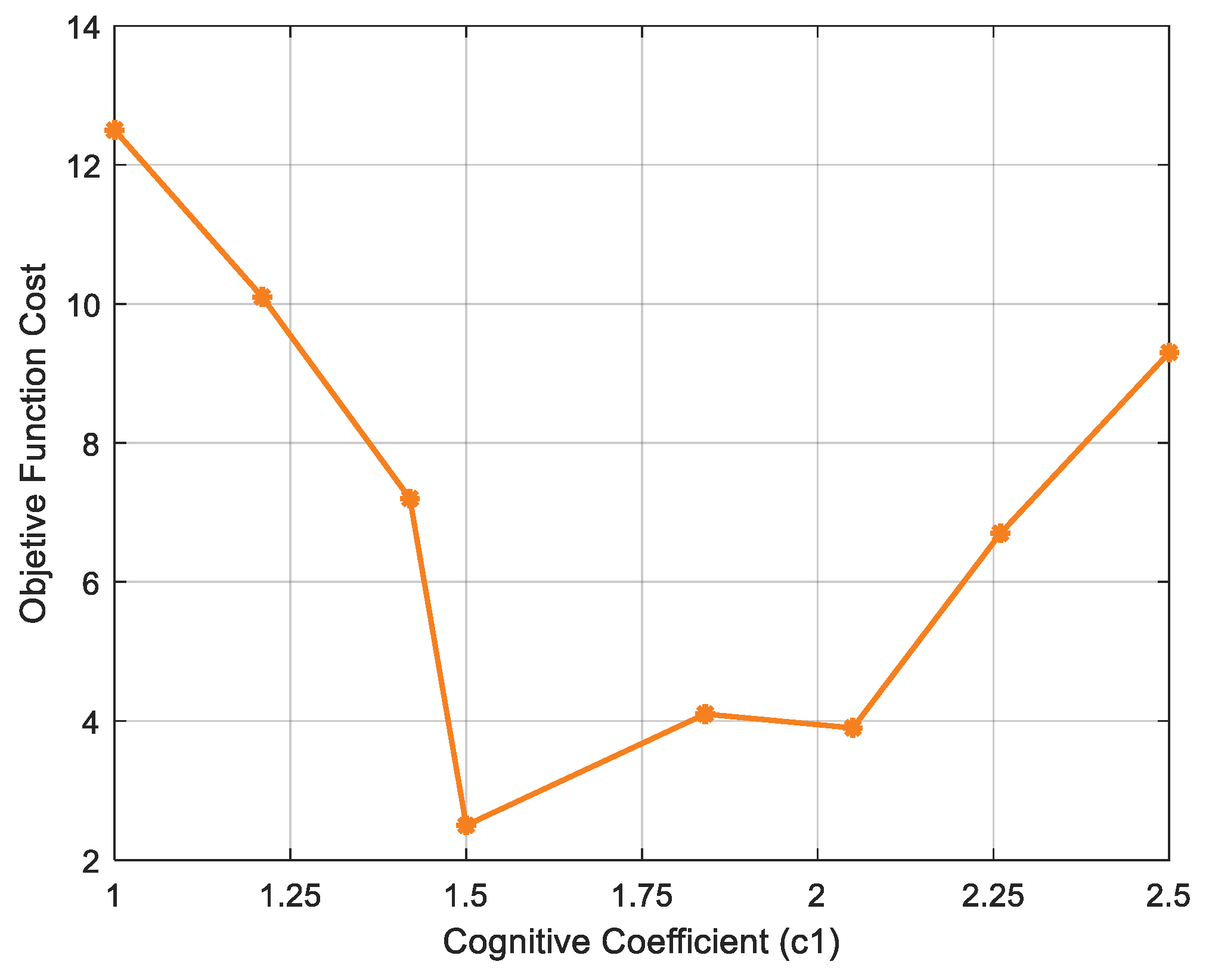
A high value of w promotes broader exploration in the search space but slows convergence, as seen with values such as 0.88 and 0.9. While a low value of w induces more conservative behavior, exploiting promising areas once identified, it can cause premature convergence, as seen in values such as 0.4, 0.48, and 0.56. Therefore, a value of w equal to 0.72 is selected for the algorithm, as it achieves the minimum cost of the objective function and, hence, a balance between exploration and exploitation. This value is reduced by 1% for each iteration until it reaches a value of w equal to 0.48. Progressive damping is applied, favoring exploration in the early iterations and ensuring exploitation when reaching the final iterations, to optimize the particle solution set. Cognitive coefficient ($c_1$): Regulates the degree of influence exerted by the best individual position achieved by each particle (pbst). It represents the individual learning tendency regarding the future trajectory of each particle. It is typically set within a range of [1–2.5]. Eight random values for $c_1$ are evaluated within the optimal range of [1, 2.5], with a fixed value of 0.72 for w, ignoring $c_2$ and $\lambda$, in an attempt to achieve the lowest cost for the objective function.

Values to be evaluated: [1, 1.21, 1.42, 1.5, 1.84, 2.05, 2.26, 2.5]

Figure 23 illustrates the high initial cost of the objective function, with $c_1$ initially set to 1. However, the price decreases until it reaches its minimum at $c_1$ = 1.5. As this value increases until $c_1$ equals 2.5, an increase in the cost of the objective function is observed, indicating that the function parameters are no longer being met and, therefore, are undesirable values for configuring the algorithm.

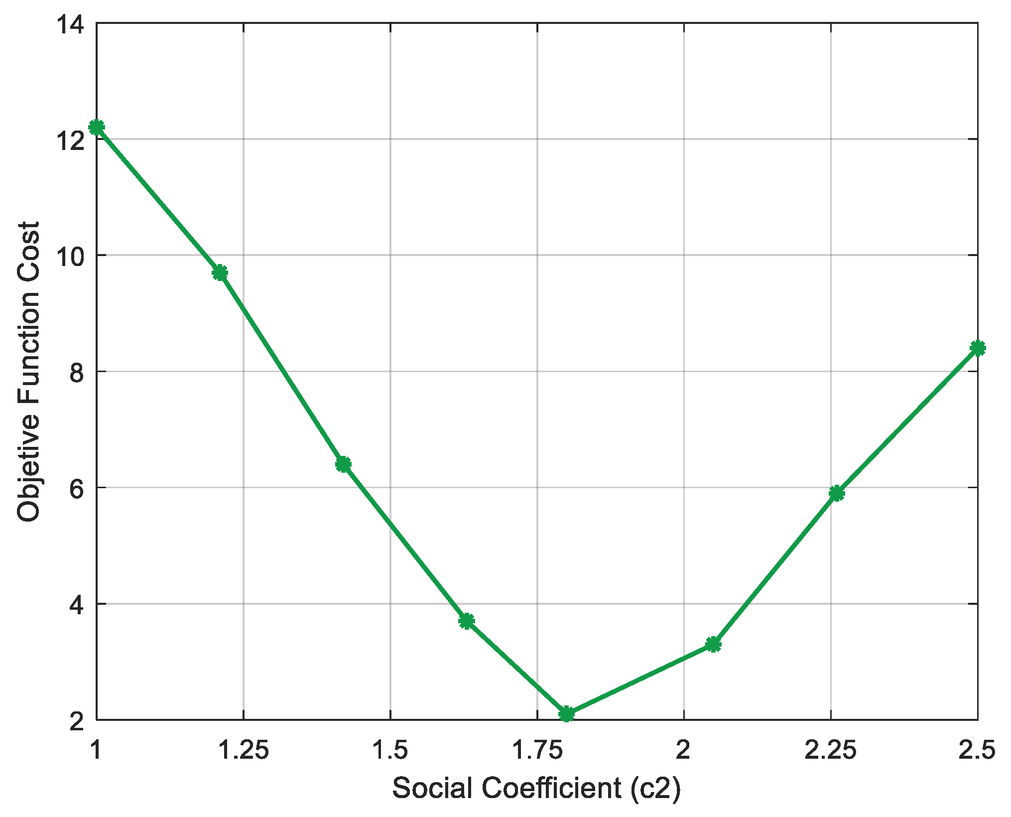
High values of $c_1$, such as 1.84, 2.05, 2.26, and 2.5, make the particle overly dependent on its own experience, preventing it from exploring new solutions. This leads to premature convergence due to stagnation in local minima, increasing the cost of the objective function. Low values of $c_1$, such as 1, 1.21, and 1.42, limit individual search and reduce the importance of the best individual position. Thus, the appropriate value for setting the parameter is $c_1$ equal to 1.5, as it allows particles to leverage their history of success without compromising the swarm’s diversity, as demonstrated by its low objective function cost. Social coefficient ($c_2$): Regulates the social learning component, representing a particle’s tendency to follow the collective knowledge of the swarm (gbst). As with $c_1$, it is usually set within a range of [1–2.5], following established criteria for evaluating parameter sensitivity. Eight random values for $c_2$ are reviewed within the optimal range of [1–2.5], with a fixed value of 0.72 for w, 1.5 for $c_1$, and ignoring $\lambda$, with the aim of achieving the lowest cost for the objective function.

Values to be evaluated: [1, 1.21, 1.42, 1.63, 1.80, 2.05, 2.26, 2.5]

As shown in Figure 24, the cost of the objective function is high, starting with a value of $c_2$ equal to 1, but this decreases as the value of $c_2$ increases until it reaches a minimum cost of $c_2$ equal to 1.80. From that point on, the price of the objective function increases again until the maximum value of $c_2$ is reached.

High values for $c_2$, such as 2.05, 2.26, and 2.5, cause a loss of diversity in the swarm, leading to premature stagnation. Low values for $c_2$, such as 1, 1.21, 1.42, and 1.63, reduce swarm coordination, resulting in slow and unstable but diverse convergence. Typically, the values of $c_1$ and $c_2$ are set equal to ensure symmetry in population exploration and avoid bias toward the nearest global optimum. 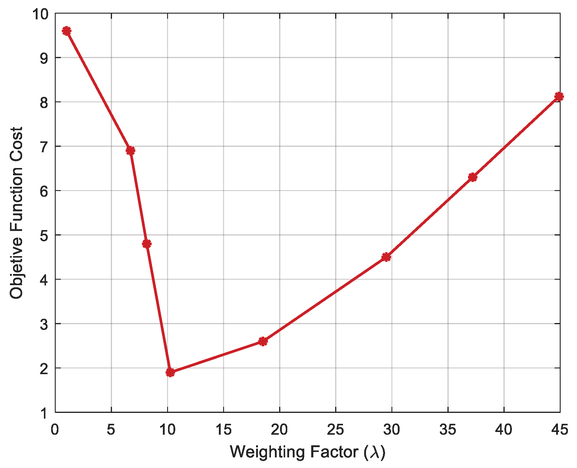However, when evaluating the different values of $c_2$ for the objective function, the value with the lowest cost is a $c_2$ equal to 1.80, indicating that there is a tendency to prioritize the global optimal solution over individual solutions, maintaining a balance between personal exploration and group collaboration, as its value is not far from $c_1$’s value of 1.5. Weighting factor ($\lambda$): This factor accounts for the error of the fundamental component in the objective function. It ensures a balance by maintaining the importance of eliminating harmonics of interest, without neglecting the magnitude of the essential component. Among the evaluated values (Figure 25), $\lambda =10$ resulted in the lowest cost for the objective function, indicating an optimal trade-off between harmonic suppression and preservation of the fundamental component. A lower $\lambda$ overemphasizes harmonic elimination, risking deviation of the fundamental magnitude, while a higher $\lambda$ prioritizes fundamental retention at the expense of residual harmonic content. Therefore, $\lambda$ = 10 ensures that both objectives are balanced effectively.

The appropriate range of values is [1–50] (

Table 6. Behavior ranges for $\lambda$.

Range of $\mathit{\lambda }$	Behavior
1–5	High priority on harmonic elimination.
5–20	Balance between THDv and fundamental component.
20–50	High priority on fundamental components.
>50	THDv is deprioritized.

Tested Values: [1, 6.70, 8.15, 10, 18.51, 29.50, 37.20, 44.90].

), depending on the priority given to the function’s objectives. For this case, eight random values spanning all working ranges of $\lambda$ will be evaluated to assess the cost of the objective function.

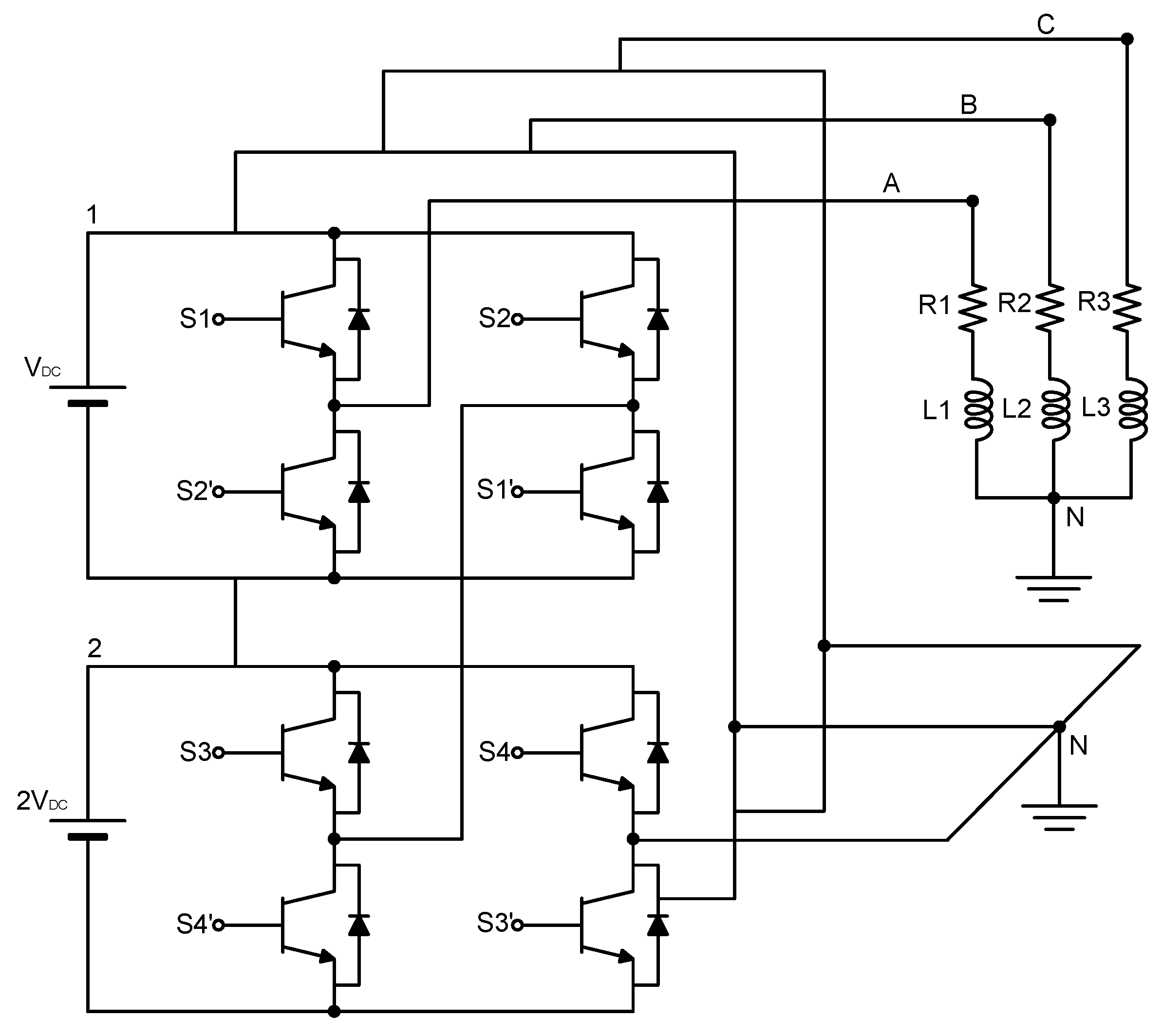
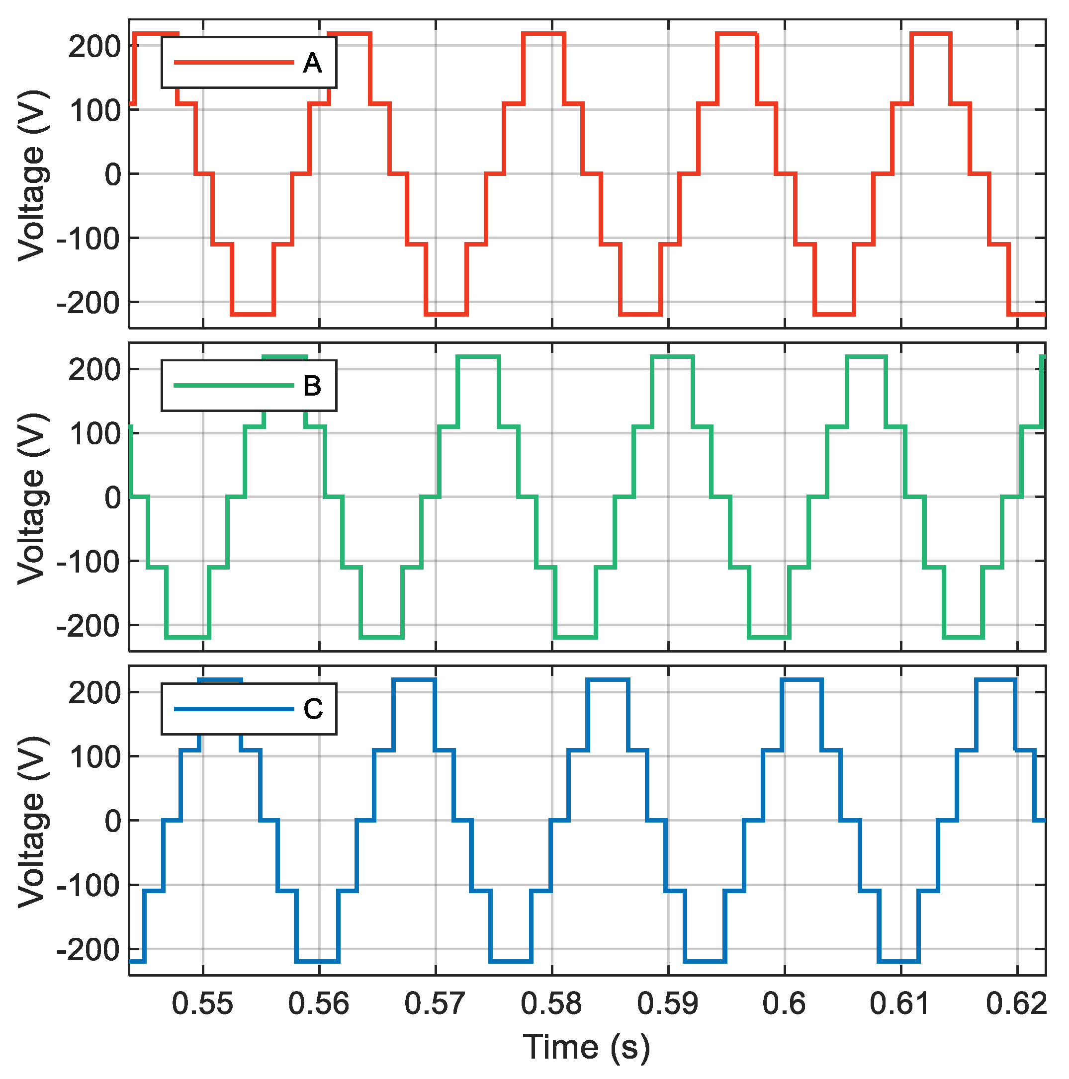
Figure 25 shows how values outside the range [5–20] present a high cost of the objective function, and within this range, the lowest cost of the objective function is found for a value of $\lambda$ equal to 10. Thus, the value used to configure the algorithm will be $\lambda$ equal to 10, as this guarantees a balance between the function objectives, thus achieving a solution consistent to reduce distortion in the CHB-MLI voltage signals.

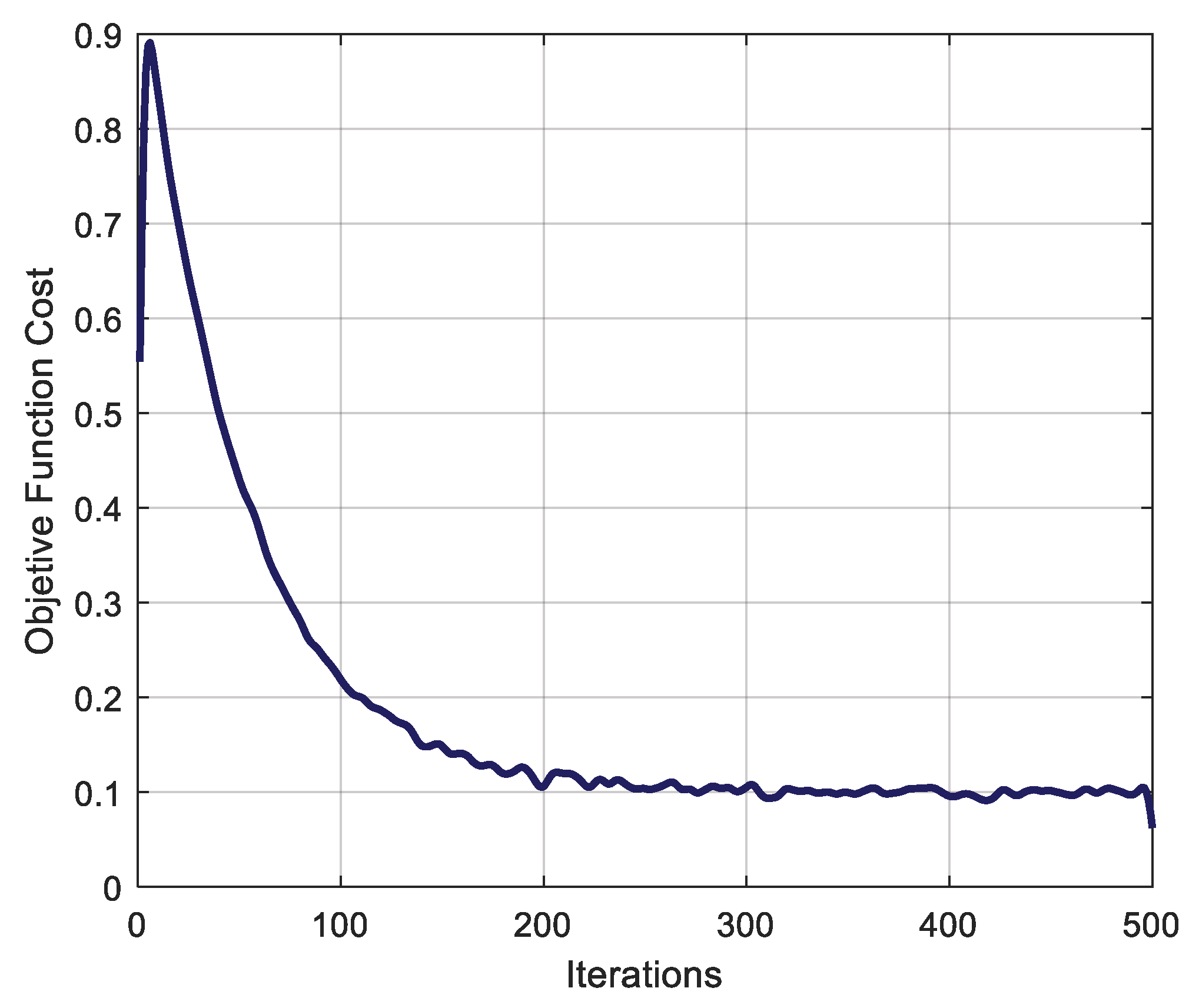
Search limits for optimal angles: lb (minimum) and lu (maximum) are set between $0.1°$ and $89.9°$, as the objective is to operate in the first quarter-wave of the voltage signal, which corresponds to a maximum value of $\pi /2$ or $90°$. However, to avoid generating conflicts in the algorithm due to divisions by zero, extreme values are avoided for the configuration. Number of particles (N): Represents the number of solutions evaluated simultaneously in each iteration. PSO typically works with a range of [30–50] particles for nonlinear optimization problems, as is the case for SHE-PWM modulation. Therefore, to avoid excessive computational load and maintain adequate search diversity, and considering that the response with the most particles is for the 9-level CHB-MLI, which requires four optimal firing angles, the value of N is considered equal to 40 to configure the parameter. Maximum number of iterations (Iter): Defines how many times the positions and velocities of the particles in the swarm are updated, ensuring that the objective function stabilizes. 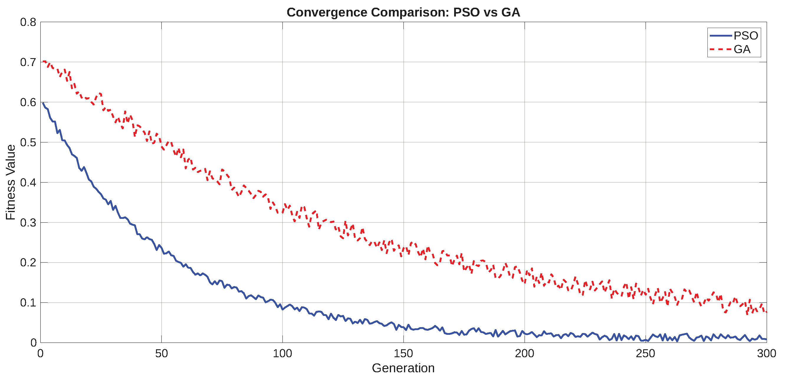Figure 26 shows how, starting at 200 iterations, the cost of the objective function begins to stabilize. After that, increasing the number of iterations does not guarantee significant improvements in the result, but it does increase the computational time of the algorithm, making it slower.

Therefore, a value below 200 iterations does not ensure convergence to stable solutions, and a value above 400 does not improve the results. Therefore, an Iter value of 300 is considered, striking a balance between solution quality and reasonable computational cost. The parameters are set to the values described in

Table 7. PSO algorithm parameters.

Parameter	Value
w	0.72
$c_1$	1.5
$c_2$	1.8
$\lambda$	10
N	40
Iterations	300
Lower bound ($lb$)	0.1
Upper bound ($ub$)	89.9

.

The selection of PSO parameters (e.g., inertia weight $\omega =0.72$, $c_1=1.5$, $c_2=1.8$) is based on sensitivity analysis results illustrated in Figure 22, Figure 23 and Figure 24. These values achieve the lowest objective function cost and ensure a balance between exploration and exploitation in the search space. Similar configurations have also been recommended in the literature for SHE-PWM optimization problems [12,13], confirming the robustness and convergence effectiveness of this parameter set.

3.3.6. Three-Phase Five-Level CHB-MLI with SHE-PWM

After solving the nonlinear system using the proposed algorithm, the following switching angles were obtained:

$${\theta }_1=32.9946°{\theta }_2=87.0270°$$

The switching times are calculated as follows:

$$t_k={\displaystyle \frac{{\theta }_k}{360}}·{\displaystyle \frac{1}{f}}$$

(29)

Therefore, assuming $f=60$ Hz:

$$t_0=0\mathrm{ms}\mathrm{and}{t}_f={\displaystyle \frac{T}{4}}\approx 4.17\mathrm{ms}$$

$$t_1={\displaystyle \frac{{\theta }_1}{360}}·{\displaystyle \frac{1}{60}}\approx 1.528\mathrm{ms}{t}_2={\displaystyle \frac{{\theta }_2}{360}}·{\displaystyle \frac{1}{60}}\approx 4.029\mathrm{ms}$$

With the calculated times, the switches are activated, thus altering the waveform of the voltage output signals, as shown in Figure 27, to reduce the percentage of voltage THDv presented by the first case study with the standard S-PWM modulation technique.

In Figure 28, it can be observed that when obtaining the signal spectrum through Fourier analysis, the percentage of voltage THDv present after implementing the hybrid methodology is 2.12%. Thus, it can be verified that the 5-level CHB-MLI generates a voltage output signal that is within the limits of national regulation [16].

Figure 29 shows that the 3rd and 7th harmonics have significantly reduced their amplitude, in addition to the fact that most of the odd harmonics that make up the signal now have an amplitude less than 1V, which is corroborated by the THDv value obtained.

3.3.7. Three-Phase Seven-Level CHB-MLI with SHE-PWM

The algorithm produced the following values for the switching angles:

$${\theta }_1=22.5963°{\theta }_2=36.0882°{\theta }_3=44.4694°$$

The corresponding switching times derived from these angles are:

$$t_1=1.046\mathrm{ms}{t}_2=1.671\mathrm{ms}{t}_3=2.059\mathrm{ms}$$

These values are used to generate the timing vectors that control the inverter switches, producing the output voltage signals. The resulting voltage levels are shown in Figure 30, where the generated voltage levels can be observed. This configuration will later be compared to its counterpart modulated using S-PWM in the following section.

These signals present a voltage THDv of 2.04%, as indicated in Figure 31, which is already accepted by national regulations, yielding a result consistent with the incidence of harmonics observed in the signal’s frequency spectrum.

As shown in Figure 32, the presence of the 3rd, 7th, and 9th harmonics is significantly reduced because, with the implemented modulation, the amplitude of the lower-order odd harmonics is below 1 V.

3.3.8. Three-Phase Nine-Level CHB-MLI with SHE-PWM

The solution of the nonlinear equations using the PSO algorithm resulted in the following switching angles:

$${\theta }_1=11.4123°{\theta }_2=17.2649°{\theta }_3=33.9502°{\theta }_4=88.7231°$$

Therefore, the corresponding switching times to activate the H-bridge cell switches are:

$$t_1=0.5283\mathrm{ms}{t}_2=0.7993\mathrm{ms}{t}_3=1.571\mathrm{ms}{t}_4=4.107\mathrm{ms}$$

These time values are used for switching the devices of each H-bridge cell through the MATLAB/Simulink block Repeating Sequence, which requires a time vector to generate the proposed SHE-PWM control signal. As a result, the output voltage waveforms shown in Figure 33 are obtained, featuring smoother voltage level transitions compared to the S-PWM-based case study.

The voltage THDv percentage, as expressed in Figure 34 after Fourier analysis, yields a desirable value within the limits of the national regulation [16], which is 1.40%.

Figure 35 shows that all the lower-order harmonics have an amplitude of less than 1 V, reflecting the low voltage THDv achieved with the implementation of the hybrid methodology developed.

4. Analysis Results

This section presents the results obtained in each case study, providing a comparative analysis between the before-and-after implementation of the hybrid SHE-PWM plus PSO methodology to reduce voltage THDv percentages in three-phase CHB-MLI inverters of varying levels. The aim is to present this methodology as an alternative to traditional modulations, such as the S-PWM that was initially used. Power quality regulations establish clear limits for the THDv percentage, as is the case with national regulation ARCERNNR 002/20, which establishes a maximum THDv percentage value of 8% for low-voltage systems, which is the case of interest for this article. No reference is made to specific values for each harmonic order. Still, it is indicated that they should not exceed 5% of the individual harmonic distortion factor concerning the voltage amplitude of the fundamental component. The regulation stipulates that if this limit is not met, the installation may be excluded from the grid, and the distributor may be penalized financially, with a value corresponding to 20 SBU per non-compliance index. It is worth mentioning that, in the case studies where the developed methodology was not implemented, none of the voltage THDv percentages meet the 8% THDv percentage limit established by national regulations.

4.1. Case 1

The five-level CHB-MLI three-phase inverter presents a high voltage THDv percentage of 20.05%, violating national regulations, when controlling breaker tripping using the S-PWM technique, as it does not prioritize suppressing harmonics but only generates a sinusoidal-like waveform at the established operating voltage levels. However, the proposed methodology not only focuses on suppressing the harmonics that have the greatest impact on increasing the voltage THDv for this case, as indicated in previous sections, but also finds the optimal angles within the set of possible solutions thanks to the PSO formulation, resulting in a THDv percentage equal to 2.12%, which complies with national regulations. As shown in

Table 8. THDv percentage and most prominent harmonics.

Indicator	S-PWM	SHE-PWM + PSO
THDv (%)	20.05	2.12
Most prominent harmonics	3, 7	None significant
Regulatory compliance	No	Yes

, the voltage THDv percentage achieved with the implemented methodology improves significantly, reaching 17.93% compared to not using it in the five-level voltage structure.

The results obtained with this methodology are significantly more favorable than those without it, consistent with what was expected from the theory developed in previous chapters, thus demonstrating that its value lies within the limits stipulated by national regulation [16].

Table 9. Harmonic amplitude in the five-level CHB-MLI according to modulation technique.

Harmonic Order	S-PWM Amplitude (V)	SHE-PWM + PSO Amplitude (V)
1st	215.6	218.0
3rd	37.61	0.78
5th	2.13	0.65
7th	7.01	0.27
9th	21.04	0.38
11th	21.91	0.41
13th	10.54	0.23
15th	2.18	0.14

compares the amplitude of the lower-order odd harmonics with S-PWM and SHE-PWM plus PSO, observing a notable reduction in their voltage amplitudes, which positively impacts the power quality supplied by this inverter.

Considering the amplitude value of 215.6 V for the 1st harmonic with S-PWM modulation, it can be verified that the 3rd, 9th, and 11th harmonics comprising the voltage signal do not comply with the individual harmonic distortion factor, exceeding the limit of 5% concerning the amplitude of their fundamental component, as indicated by national regulations. In this case, this limit is a maximum of 10.78 V. Therefore, it can be verified that this indicator is not met. Due to the restriction on the number of angles that can be worked with, only two firing angles can be obtained in this case; therefore, the two harmonics of interest are suppressed. However, because the objective function prioritizes global optimization results thanks to the $c_2$ configuration, the remaining lower-order odd harmonics are also reduced, thus ensuring a low THDv value. The new harmonics, achieved through the firing angles obtained with SHE-PWM modulation and PSO, ensure compliance with the individual harmonic distortion factor (THDv). As shown in Table 9, none of them exceeds the amplitude value of 10.9 V, which is the limit of 5% for the value of a fundamental component of 218 V. While the five-level CHB-MLI inverter achieves a THDv of 2.12%, which is well below the regulatory limit, it is still higher than the 1.40% of the nine-level configuration. This can be attributed to the THDv being bound by the number of levels in the configuration; a five-level configuration has higher step resolution distortion due to fewer levels, which translates to increased step resolution distortion. The five-level configuration is severely limited by hardware to only two firing angles. This is far less than the nine-level configuration (four firing angles), and thus the five-level structure can no longer suppress additional harmonics and is severely limited in distortion reduction due to hardware and structure of the inverter.

4.2. Case 2

This is the structure of the seven-level CHB-MLI three-phase inverter, where S-PWM modulation results in a voltage THDv percentage of 13.68%. This, compared to the 5-level inverter with the same topology, presents an improvement. However, it still violates national regulations, since the THDv value does not fall within the limit stipulated by them. This confirms the theory that increasing the levels in an inverter makes its signal more similar to the desired sinusoidal signal (

Table 10. THDv percentage and most prominent harmonics.

Indicator	S-PWM	SHE-PWM + PSO
THDv (%)	13.68	2.04
Most prominent harmonics	3, 7, 9	None significant
Regulatory compliance	No	Yes

).

The THDv percentage achieved with the SHE-PWM plus PSO technique is 2.04%, thus complying with national regulation [16], and it shows an 11.64% improvement compared to S-PWM modulation. This demonstrates that, despite the reduction in intrinsic THDv due to the increased number of voltage levels, it is still possible to improve signal quality by implementing a suitable modulation technique, such as the one developed in this article.

Table 11. Harmonic amplitude in the seven-level CHB-MLI according to modulation technique.

Harmonic Order	S-PWM Amplitude (V)	SHE-PWM + PSO Amplitude (V)
1st	217.2	220.0
3rd	23.01	0.83
5th	1.23	0.64
7th	9.96	0.72
9th	7.48	0.71
11th	1.96	0.66
13th	2.03	0.92
15th	13.54	0.33

compares the amplitude of the lower-order odd harmonics with S-PWM and SHE-PWM plus PSO, showing a notable reduction in their voltage amplitudes, which results in an improvement in the power quality supplied by this inverter model.

Considering the individual harmonic distortion factor, S-PWM modulation reveals harmonics with an amplitude value greater than 10.86 V, which is the corresponding limit of 5% for a fundamental component amplitude value of 217.2 V, such as the 3rd and 15th harmonics, thus failing to comply with this indicator. Performing the same analysis for SHE-PWM plus PSO modulation, it can be verified that none of the voltage amplitudes of the harmonics that make up this signal exceed 11 V, which is the corresponding limit of 5% for a 220 V amplitude. The result obtained shows a THDv percentage that is admissible according to the national regulation on which the presented article is based, in addition to complying with the harmonic distortion factor for each harmonic component of the signal.

4.3. Case 3

For the nine-level CHB-MLI three-phase inverter structure, the voltage signals delivered with standard S-PWM modulation present a THDv percentage of 10.40%. This value does not comply with national regulations. However, it indicates an improvement in the distortion of the supplied voltage signals compared to the five- and seven-level case studies with the same modulation.

Table 12. THDv percentage and most significant harmonics.

Indicator	S-PWM	SHE-PWM + PSO
%THDv	10.40	1.40
Dominant Harmonics	3, 7, 9, 13	None are significant
Regulation Compliance	NO	YES

shows the voltage THDv percentage achieved by implementing the hybrid methodology, which is 1.40%, representing a 9% improvement compared to the THDv achieved with S-PWM modulation. It should be noted that the decrease from 10.40% (S-PWM) to 1.40% (SHE-PWM + PSO) THDv on the nine-level CHB-MLI inverter is not only a technical achievement regarding the improvement of the waveform but also demonstrates adherence to the ARCERNNR 002/20 standard. This standard imposes a maximum allowable THDv of 8% for low-voltage systems, and non-compliance may attract administrative fines of 20 SBU for each breached point and a potential disconnection from the grid. Thus, this 9.0% improvement (compared to S-PWM) is a considerable, risk-free engineering advance without the possibility of incurring fines, supporting safe grid integration and ensuring the long-term reliability of the device.

The THDv achieved in the voltage output signals using the SHE-PWM plus PSO modulation technique is a percentage value that complies with national regulation [16], as it is below the 8% limit mentioned for low-voltage systems.

Table 13. Harmonic amplitudes in the 9-level CHB-MLI according to modulation technique.

Harmonic Order	S-PWM Amplitude (V)	SHE-PWM + PSO Amplitude (V)
1st	218.2	220
3rd	16.19	0.68
5th	0.39	0.24
7th	8.43	0.74
9th	2.29	0.17
11th	0.17	0.09
13th	6.18	0.16
15th	3.24	0.10

compares the amplitude of the lower-order odd harmonics with S-PWM and SHE-PWM plus PSO, showing a notable reduction in their voltage amplitudes, which results in an improvement in the quality of the supplied power.

Evaluating the individual harmonic distortion factor for S-PWM modulation, it can be observed that the third harmonic exceeds the voltage amplitude value of 10.91 V, which corresponds to 5% of a fundamental voltage amplitude component of 218.2 V. The voltage amplitude of all odd-order lower harmonics after modulation with the SHE-PWM plus PSO technique results in a value less than 1 V. Therefore, the national regulation for the individual harmonic distortion factor is met, since a voltage amplitude of 11 V is not exceeded, which is equivalent to 5% of the limit for a fundamental voltage amplitude component of 220 V. This case study presents the best waveform in the voltage output signal, both with and without the methodology implemented, as shown in Figure 19 and Figure 33, respectively. Although S-PWM modulation achieves a THDv value of 10.40%, it does not meet the 8% limit specified in the national regulation [16] for low-voltage systems. Comparing the voltage amplitude values of the fundamental component or 1st harmonic across all case studies reveals an improvement in its value, both with increasing levels and with the use of SHE-PWM plus PSO modulation, as its values become increasingly closer to the corresponding peak amplitude of 220 V. Therefore, implementing the methodology is crucial to meet the THDv percentage requirement specified in the regulation. Hence, the value achieved with the SHE-PWM plus PSO technique of 1.40% verifies the efficiency of this methodology in reducing THDv and maintaining an adequate value in its fundamental component, with almost no energy dispersion in the lower-order odd harmonics that comprise the voltage output signals for this case study. A comparison is made between the THDv percentages of all the case studies with and without the application of the hybrid SHE-PWM plus PSO methodology, as detailed in

Table 14. THDv comparison for the case studies.

Inverter Levels (S-PWM)	THDv (%)	Inverter Levels (SHE-PWM + PSO)	THDv (%)
5	20.05	5	2.12
7	13.68	7	2.04
9	10.40	9	1.40

and Figure 36.

Figure 37 illustrates the proximity of each inverter model to the limit set by national regulations for each THDv percentage. It shows that with standard S-PWM modulation, the limit was exceeded with values of up to 12.05% in the case with the highest THDv. Meanwhile, with SHE-PWM modulation plus PSO, THDv values up to 6.60% below the national regulation limit were achieved for the case with the lowest THDv.

In cases where the hybrid methodology is not implemented, a reduction in the voltage THDv percentage is only evident thanks to the increase in voltage levels. As mentioned in previous chapters, the greater the number of voltage levels an inverter model is capable of generating, the smoother the signal it delivers will be, with transitions between each voltage level more closely resembling the desired sinusoidal waveform. In cases where the hybrid methodology is implemented, a significant reduction in the THDv percentages in the inverter models’ output signals is evident. A similar THDv value is maintained for the three case studies with SHE-PWM modulation. Figure 38a,b show the profile of key characteristics for each inverter model, such as the percentage of THDv, the highest harmonic amplitude, the percentage of the voltage profile, the number of DC voltage sources, and their value. This is true for each case study and each modulation technique: S-PWM and SHE-PWM, respectively, along with PSO. The behavior can be observed based on the number of levels of each proposed CHB-MLI, relating the percentage of THDv and the highest-amplitude harmonic to the voltage level of the DC sources and the number used by each inverter. It is shown that for S-PWM modulation, this directly influences the increase in the percentage of THDv. In contrast, with SHE-PWM plus PSO modulation, achieving a low THDv rate is irrelevant, as it focuses on incident harmonics and the correct implementation of the objective function in the developed algorithm.

In conclusion, the chapter examines the impact of the results, specifically the effect of minimizing total harmonic distortion (THDv) in multilevel three-phase inverters. This has significant technical implications for real-world electrical systems, especially in industrial and distributed generation applications. Reducing THDv directly translates into several technical benefits, such as the following. Improved power quality: A lower THDv brings the inverter signal closer to a pure sinusoidal shape, which improves power transmission, reduces heat losses in electrical equipment, and prolongs its lifespan. Reduced motor heating and vibration: A low THDv improves the dynamic and thermal behavior of this equipment, reducing the generation of pulsating torques. Increased system efficiency: By reducing THDv, losses in lines, transformers, and capacitors are minimized, and the system’s power factor is optimized. Reduced use of external filters: Generating a high-quality signal minimizes the need for passive filters to mitigate harmonics, simplifying system design and lowering implementation costs. Additionally, complying with national regulations prevents financial penalties and system isolation from the grid.

4.4. Comparative Evaluation of Optimization Algorithms

To evaluate the effectiveness of the proposed hybrid SHE-PWM + PSO approach, a comparative study was conducted using the Genetic Algorithm (GA) under the same optimization framework. Both algorithms were tested on the seven-level CHB-MLI inverter, targeting the elimination of the 3rd, 7th, and 9th harmonics, with a modulation index of $m=1$.

The configuration parameters—population size (40), iteration count (300), and search bounds—were kept identical for both cases. The genetic algorithm converged to a final fitness of approximately 0.50716, exhibiting a more gradual approach to saturation, which occurred only after approximately eighty generations, as shown in Figure 39b. Figure 39a presents the harmonic spectrum, which reveals a persistent presence of low- and mid-order harmonics; specifically, the 3rd, 7th, and 14th harmonics exhibit voltage amplitudes that, in certain instances, surpass 150 V. These findings confirm that, although the genetic algorithm achieves a reduction in total harmonic distortion, it falls short of the particle swarm optimization method in entirely suppressing critical harmonics and in preserving a high-quality spectral profile.

In contrast, the PSO-based method achieved superior harmonic suppression, with total harmonic distortion (THDv) reduced to 2.04%, compared to 3.81% for GA.

Table 15. Comparison of PSO and GA optimization results for the 7-level CHB-MLI inverter.

Metric	PSO	GA	Improvement (%)
THDv (%)	2.04	3.81	46.45
Execution Time (s)	8.34	12.67	34.18
Fundamental Component (V)	220.0	217.3	–
Convergence Iterations	196	282	–

summarizes the quantitative results.

These findings confirm the robustness and efficiency of the PSO approach in solving nonlinear harmonic elimination problems in multilevel inverters. It offers better convergence speed and more consistent harmonic attenuation, especially for lower-order harmonics, making it highly suitable for embedded and real-time applications.

These results validate the suitability of PSO for solving the nonlinear SHE-PWM problem in CHB-MLI inverters, particularly for real-time or embedded applications where convergence speed and accuracy are critical, stabilizing after about 80 generations (see convergence plot in Figure 39b. As seen in Figure 39a, both Particle Swarm Optimization (PSO) and Genetic Algorithm (GA) were applied to the seven-level CHB-MLI switching angle optimization problem to examine their convergence behavior. It is evident that PSO outperformed GA in terms if convergence speed and the optimization problem’s generation count relative to the achieved stable fitness value, Figure 40. PSO reached a stable and lower fitness value in roughly 80 generations, while GA continued a more gradual decline while hovering around a higher fitness level.

This behavior emphasizes PSO’s effectiveness in nonlinear equation optimizations like SHE-PWM. PSO’s consistent convergence stability is a significant benefit for real-time embedded systems, where computational time and solution accuracy are critical metrics. Moreover, with the optimized parameters ($c_1=1.5$, $c_2=1.8$, $\lambda =10$), PSO yielded a greater preservation of the fundamental component while restricting the selection of harmonic minimization due to its balance of exploitability of convergence.

As provided in Equation (28), the PSO and GA fitness functions were defined to include the squared error of the harmonic components concerning the desired modulation index. Moreover, the data provided in Table 15 indicate a 46.45% improvement in THDv. This, along with the observed superior convergence behavior of PSO, further supports its relative advantage for this class of optimization in the application of multilevel inverters.

5. Conclusions

Simulation of the five-, seven-, and nine-level three-phase inverter models using the CHB-MLI topology revealed that, despite generating voltage output signals of considerable quality, they exhibit high levels of Total Harmonic Distortion (THDv) when employing conventional modulation techniques, such as S-PWM. With this modulation, a minimum THDv value of 10.40% was achieved in the nine-level inverter, exceeding the regulatory limit established by national regulation [16] by 2.40%, which is the maximum threshold of 8%. These results demonstrate that the S-PWM modulation used in the initial case studies is not sufficient to guarantee regulatory compliance.

The implementation of the optimized SHE-PWM technique using PSO enabled the generation of optimal switching angles that significantly reduced the THDv in all case studies. Although the selected harmonics were not eliminated, the methodology managed to reduce their amplitudes to values below 1 V, thereby improving the spectral profile of the voltage output signals for each inverter and meeting the individual harmonic distortion factor (HDF) of less than 5% of the fundamental component amplitude, which, for a value of 220 V, cannot exceed individual amplitudes of 11 V. This performance was achieved thanks to the formulation of an appropriate objective function and parameter configuration so that the PSO prioritizes global solutions, establishing a higher value for the social coefficient than for the cognitive coefficient.

The developed objective function guaranteed both the preservation of the fundamental component and the efficient suppression of lower-order odd harmonics, achieving an optimal solution and obtaining the appropriate firing angles for each case study. The switching angles enabled the construction of precise time vectors, allowing for the generation of control signals that preserved the peak value of the first harmonic at approximately 220 V. This indicates minimal energy dispersion in the other lower-order harmonics, thus ensuring a voltage supply delivered by the inverters with a correct peak voltage value and low harmonic distortion of the signals.

The application of the hybrid SHE-PWM plus PSO methodology allowed the three simulated CHB-MLI inverter models to comply with the limits established by national regulation [16] for THDv percentages in low-voltage systems. The THDv percentage results achieved for case studies 1, 2, and 3 were 2.12%, 2.04%, and 1.40%, respectively, representing measurable improvements of 17.93%, 11.64%, and 9% compared to standard S-PWM modulation. Furthermore, the THDv values obtained with the implemented methodology were below the regulatory limit by margins of 5.88%, 5.96%, and 6.60% for the CHB-MLIs of five, seven, and nine levels, respectively.

The combination of SHE-PWM with PSO has proven to be a versatile, scalable, and effective solution for reducing THDv in multilevel three-phase inverters. Its architecture allows for expansion to more complex configurations without requiring a redesign of the control system. Thus, the developed methodology is adaptable to multiple application environments, including renewable energy conversion systems, industrial drives, microgrids, e-mobility systems, and HVDC links. The hybrid algorithm’s ability to dynamically adjust to different constraints and operating conditions highlights its value as a flexible, robust, and multi-objective tool for improving power quality in real-world electrical systems, both at low and high voltages.

Future Work

Building on the encouraging outcomes produced by the hybrid SHE-PWM and PSO strategy applied to CHB-MLI three-phase inverters, the data reported here derive from idealized and rigorously controlled simulation scenarios. Thus, attention is directed toward subsequent investigations and experimental studies that will expand on the following focal areas:

• The deployment and experimental validation of the SHE-PWM and PSO strategy on real-time embedded platforms, including DSPs and FPGAs, where rapid sample rates and low-latency PWM generation are essential for stable operation in dynamic, grid-connected settings.
• The fusion of edge intelligence and adaptive control through machine-learning-augmented metaheuristics, which will facilitate the real-time adjustment of switching angles in response to fluctuating load conditions, evolving harmonic constraints, and stringent grid-code requirements in smart inverters and energy-optimized applications.