Abstract
Heating, ventilation, and air-conditioning (HVAC); domestic and commercial buildings; district energy; industrial processes and water treatment; municipal wastewater and water supply; and agriculture and irrigation, among others, represent a wide breadth of domains where pumps are used. From this perspective, the number of pumps that will be required to ensure future human demands is expected to increase significantly; accordingly, power consumption is also expected to increase sharply. Therefore, the energy efficiency of pumps will become an even more important topic of concern when designing a pumping installation. The objective of the present study is to introduce a user-friendly Excel workbook that enables the design of pumping systems with centrifugal pumps. It was initially conceived for use in Hydraulic Machines Master’s lectures, but its use might be examined from a wider perspective. The workbook includes 22 worksheets, all linked to each other, addressing different aspects of the design. Special attention is given to the calculation of the major and minor head losses, to the cavitation phenomenon, to the use of dimensionless coefficients to determine the rotation speed to obtain a specific operating point, and to the calculation of the system curve. Today, energy efficiency represents an important goal in every pumping facility; therefore, one of the objectives of this tool is to enable the user to quantify both the shaft power and the efficiency of different operating points, thus allowing a sustained definition of the best solution.
1. Introduction
Energy efficiency is a top-priority topic in current times, namely in the engineering domain. This importance may even escalate significantly in the future, particularly as energy demand is expected to increase. The design of energy-efficient systems can be compared with an international competitive race, in which the winner will be better prepared to face the future. From this perspective, pumping systems will be examined as a field where energy efficiency will play as important a role as the intrinsic role the pump itself plays. The design and pursuit of energy-efficient pumps already represent some of the main goals, if not the main goals, of pump manufacturers.
Currently, pumps are used worldwide in a very wide range of facilities, including refrigeration, air conditioning, boilers, water supply, agriculture, aquaculture, etc. One might argue that it is impossible to count the number of pumps working today or even to have a rough estimate. Accordingly, it is also impossible to have an idea of the power demand that pumps are requiring today; perhaps even more difficult is to be aware of typical efficiency values. Across the lifecycle of a pump, the overall costs include purchase, maintenance (i.e., replacement of mechanical shaft seals, of electric motors, of impellers, etc.), daily energy expenditures, and other possible expenses. The contribution of the energy costs throughout the whole lifecycle of a pump can be very significant. Different reference values for these costs can be found in the literature, in some cases reaching up to 40% [1,2]. Therefore, the daily operation of a pump represents a topic of concern.
The present study addresses these objectives by proposing an Excel workbook entitled “EEP: Energy-Efficient Pumps Design Tool”, designed to achieve energy-efficient pumping systems. The development of applications similar to this one should not be viewed as a tool only useful to the academic community; on the contrary, the main goal is directed to real-world applicability and to the design of more energy-efficient pumping systems. However, at the same time, it may also represent a bridge between a theoretical approach, since some fundamental issues are addressed, and a practical, easy-to-use tool in the everyday life of engineers. Therefore, this Excel workbook provides a user-friendly tool for analysing and designing pumping systems. Since centrifugal pumps are widely used and probably represent the most common type of pump worldwide, the workbook was developed considering this type of pump. Pump manufacturers such as Grundfos (www.grundfos.com, accessed on 30 July 2025) have available online software that represents the state of the art in this field and enables users to select a given pump [3]. However, in terms of the design of a pumping system, this kind of online software shows some limitations, namely because the objective of manufacturers is directed to the operation of the pump itself.
This study is the result of a collaborative effort between Miguel Hernández University (UMH) of Elche, Spain, and the Coimbra Institute of Engineering (ISEC), Portugal, initiated through an Erasmus+ program in 2023. Several academic exchanges and joint activities, including student supervision and mobility periods, have supported the development of this work, particularly during the 2023–2024 academic year. The final mobility period in April 2025 was specifically focused on completing the present contribution. The present application was initially conceived for use in Hydraulic Machines Master’s lectures, but throughout its development, it was enhanced to encompass a wider perspective. In some contexts, it might be a useful tool for engineers involved in the design of pumping systems.
At the present time, the first experiences with the EEP workbook are being implemented and assessed in Spain and Portugal. In the case of the former, the EEP tool is being used in the School of Engineering of Elche of Miguel Hernández University (UMH) and, for the latter, in the Department of Mechanical Engineering of the Coimbra Institute of Engineering (ISEC) of the Polytechnic Institute of Coimbra (IPC). Table 1 lists the characteristics of the curricular units in which the workbook is currently being used.

Table 1.
Characteristics of the ISEC and UMH curricular units.
The design of pumping systems and the development of more energy-efficient pumps have been the focus of numerous recent studies. Zhang et al. [4] stated that pumps are essential in various industries, where their operational stability and efficiency are crucial. They analysed the composition and variation characteristics of hydraulic radial force on the impeller using a data-centric approach based on computational fluid dynamics (CFD) datasets, providing guidance for optimising impeller design. Nan et al. [5] proposed a hydraulic loss and convolutional neural network (HLCNN)-based approach to predict centrifugal pump energy performance. Their goal was to improve the accuracy and interpretability of the traditional centrifugal pump performance prediction (CPPP) model, which relies on semi-theoretical and semi-empirical methods. Pei et al. [6] highlighted that research on energy-efficient disc pumps is particularly important moving forward. Based on the available information from the open literature, they thoroughly reviewed the research and development of the disc pump. This study provides a new perspective for the development of energy-efficient disc pumps. Yu et al. [7] underlined that the complete characteristics of centrifugal pumps are crucial for the modelling of hydraulic transient phenomena occurring in pipe systems. Therefore, to acquire the full characteristic curves based on the manufacturer’s normal performance curve, this study proposes a machine learning (ML) model to predict full Suter curves using a pump’s specific speed with the known parts of the Suter curve. The proposed ML model combines several types of regression models in an attempt to find the most accurate prediction in terms of the root mean square error (RMSE). Pavlenko et al. [8] noted that developing ways to increase centrifugal pumps’ pressure and power characteristics is a critical problem in modern engineering. The aim of this study was to ensure higher energy-efficiency indicators by using a counter-rotating pumping stage with trimming. Based on CFD modelling and the Moore–Penrose pseudoinverse approach for overdetermined systems, a comprehensive approach was performed. Pavlenko et al. [9] investigated the improvement of energy efficiency in a new design of pumps for nuclear power plants. They stressed that the reliability of pumping units at nuclear power plants (NPPs) is critical in terms of their energy efficiency and safety. The outcome of this important study was the design and development of a promising pump with increased energy efficiency. Finally, Oliveira et al. [10], in a study that represents the starting point of the present contribution, proposed an Excel workbook that enables the design of pumping installations with centrifugal pumps.
The final version of the EEP workbook is part of this contribution and is freely available as Supplementary Material. In addition, an example of a problem statement is also made available as Supplementary Material, which is fully solved in the EEP workbook. This solved problem provides users with guidance in managing the workbook. The organisation of the workbook is presented in the next section. This is followed by the Results section, which explores several topics, with special attention to major and minor head losses. The system curve, the pump’s performance curves, the use of dimensionless coefficients, and the cavitation phenomenon are also analysed.
2. Materials and Methods: Organisation of the Workbook
The first question to be answered in the design of a pumping installation is what type of pump is required. Grundfos (www.grundfos.com, accessed on 30 July 2025), has technical solutions that include circulator pumps, booster sets, inline single-stage pumps, end-suction pumps (close coupled and long coupled), horizontal split-case pumps, multistage pumps (both inline and horizontal), immersible pumps, encapsulated pumps, submersible pumps for wastewater and groundwater, machine-tool pumps, and diaphragm pumps.
KSB (www.ksb.com, accessed on 30 July 2025), another pump manufacturer, offers designs that include horizontal volute casing single-stage pumps; horizontal, radially split ring-section multistage pumps with radial impellers (single entry or double entry); multistage vertical high-pressure centrifugal pumps with inline design; horizontal or vertical single-stage submersible motor pumps in close-coupled design; and all-stainless-steel centrifugal pumps—either single-stage or multistage—in ring-section design, suitable for vertical or horizontal installation.
Upon selecting the type of pump required for the installation under analysis, the user must have available the technical catalogue/datasheets of the models available for that type of pump. Usually, the manufacturers provide a selection diagram, where all the models, each with a specific commercial code, and their range in terms of both flowrate and head rise are shown. To start working with the Excel workbook, this data must be available.
The workbook comprises 22 worksheets. The first ones are just introductory (1_front page, 2_Nomenclature and 3_Formulas), followed by “4_Pump curve”, “5_Material”, “6_Coef._KL”, “7_System curve”, “8_Material_Flamant”, “9_Material_Hazen-Williams”, “10_Head losses”, “11_Head losses—Leq”,”12_Pump selection”, “13_Operating point (1)”, “14_Efficiency point 1”, “15_Power point 1”, “16_NPSH point 1”, “17_PPE & point 3”, “18_Point 2”, “19_Pv and Pa”, “20_Cavitation”, “21_Table 3 points + EUR”, and “22_Units”. The last worksheet allows the user to convert some of the most frequently used units in this field. The workbook is almost entirely protected, which means that no changes are allowed in most cells. Only the cells that require input data were left unprotected. This way, unintentional changes in the cells containing formulas, fixed values, or values based on calculations or data from other worksheets are avoided.
The workbook includes the following:
- -
- A comparison of equations for estimating the head losses in pipes (major losses) (Worksheet “10_Head losses”).
- -
- A comparison of equations for the estimation of the friction coefficient (λ), including explicit and implicit equations (Worksheet “10_Head losses”).
- -
- A comparison of the total head losses calculated with the reference procedure and the equivalent length method, assuming different percentages for the minor losses (Worksheet “11_Head losses—Leq”).
- -
- A procedure to obtain the system equation of a given installation (Worksheet “7_System curve”).
- -
- A procedure to calculate the rotation speed of the pump to obtain a specific operating point (Worksheet “12_Point 2”).
- -
- A procedure to perform different calculations with dimensionless coefficients (Worksheet “12_Point 2”).
- -
- A procedure to assess the occurrence of cavitation (Worksheet “20_Cavitation”).
- -
- A procedure to assess possible economic savings (Worksheet “21_Table 3 points + EUR”).
Furthermore, it is important to mention that the workbook was designed for a specific type of pumping system, namely with one suction section and two discharge sections. However, depending on the specific goals of the user, several improvements might be considered and implemented. Hence, despite the present stage of development, the workbook should be regarded as an open tool to be enhanced. Once fully developed and tested, the final goal of the “EEP: Energy-Efficient Pumps Design Tool” workbook is to be available for master and bachelor lectures in engineering schools and also for professionals working in Pumping Engineering Design Offices.
3. Results
3.1. Major Head Losses, Friction Coefficient, and Minor Head Losses
In a given system, two types of head losses must be considered: the major losses, i.e., the energy dissipation due to the pipe’s frictional resistance, and the minor losses, i.e., the energy dissipation due to local resistances in fittings/components. These designations, as major and minor, are relative, since both types of energy dissipation depend on the pipe’s length and on the number of components. In fact, in a given system, if the pipe’s length is small and the number of components is high, the relative contribution of the minor losses to the total losses might be much higher than that of the major losses. However, as stated by Lahiouel and Lahiouel [11] in water distribution and petroleum systems, the friction losses are typically higher than those that occur in fittings. Thus, the designations as major and minor correspond to the magnitude of each of the losses.
A detailed assessment of head losses in a given installation requires a thorough analysis and is cumbersome. Therefore, it is neither common nor practical. Several simplifications are thus assumed, particularly in typical engineering projects. The assumption that the minor head losses can be estimated as a given percentage of the total length of the pipe’s installation represents a good example of this approach. The concern regarding the accuracy in the calculation of the head losses is more relevant to the academic and the scientific communities than to engineers, who must deal with projects on a daily basis and often face deadlines that are too short to meet. Nevertheless, as stated by Coelho et al. [12] in a study dedicated to irrigation engineering projects, the calculation of the head losses is the most important factor to take into account. Accordingly, in the design of pumping systems—despite the low viscosity of water (reference fluid in this work) and its very low compressibility—the head losses may be significant and clearly influence the operating point of a pump and thus its power demand and efficiency. Therefore, in the present workbook, special attention is given to these issues.
A very significant number of equations are available in the literature to estimate head losses. Head losses depend on various factors, namely the temperature and viscosity of the fluid, the material, the diameter and length of the pipe, and the flow velocity. The equations to estimate the head losses are determined according to the specific flow regime —laminar or turbulent—which is defined on the basis of the Reynolds number (Re). Re represents the relationship between the inertial and the viscous forces and is calculated as follows:
where Re is the Reynolds number (dimensionless), ρ is the density [kg/m3], V is the mean velocity of the fluid in a pipe [m/s], L* is the characteristic dimension [m], μ is the dynamic viscosity [N·s/m2], and υ is the kinematic viscosity [m2/s].
The characteristic dimension (L*) corresponds, in the case of flows in circular pipes (geometry considered in this work), to the internal diameter of the pipe. In circular pipes, if Re < ≅2000, the flow is assumed to be laminar. If Re > ≅4000, the flow is turbulent, and the region between 2000≅ < Re < ≅4000 is considered as a transition zone in which both inertial and viscous forces may prevail. For the present purposes, and since in pumping systems the flow is “almost” always turbulent, this is the only flow regime considered for head loss calculations. However, if for any reason the Reynolds number is below 2000, this is highlighted in the workbook as an alert, and the corresponding cell appears red together with the word “Laminar” in red text. Otherwise, if Re is between 2000 and 4000 the word “Transition” will be shown.
In the present workbook, both major and minor head losses are considered. Among the large number of equations available to estimate friction losses, those proposed by Darcy–Weisbach, Hazen-Williams, and Flamant were selected. On the other hand, the friction coefficient is estimated with both explicit (Haaland, J.J. Chen, and Moody, which was taken as the reference) and implicit (Colebrook, with the first iteration based on the result obtained with the Moody equation) equations.
The present contribution does not intend to perform an in-depth analysis of the equations available in the literature to estimate friction losses and the friction coefficient. Examples of such an approach can be found elsewhere, for both friction losses [11,12,13,14] and the friction coefficient [15,16,17,18,19].
The Darcy–Weisbach equation, valid for any fully developed, steady, incompressible pipe flow (placed horizontally or with a slope) [20], is given by
where hf is the major head losses [m.c.H2O], λ is the friction coefficient (Moody] (dimensionless), L is the length of the pipe [m], d is the diameter of the pipe [m], V is the mean velocity of the fluid in a pipe [m/s], and g is the acceleration of gravity [m/s2].
The Hazen–Williams equation is given by [21]
where Q is the flowrate [m3/s] and CH-W is the Hazen–Williams coefficient (dimensionless).
The Flamant equation is given by [22]
where CF is the flamant coefficient (dimensionless) and d is the diameter of the pipe [mm].
The explicit equations to calculate the friction factor are the following [23,24,25]:
where ε is the roughness of the pipe wall [mm].
The implicit equation to calculate the friction factor was proposed by Colebrook–White [26]:
Despite the large number of explicit equations already available to calculate the friction coefficient, research on this topic is still ongoing. Therefore, one may conclude that the best correlation has not yet been established [19]. An exhaustive review of explicit correlations is presented by [27]. However, since 1944, when Moody plotted his chart for the friction coefficient in commercial pipes in the ranges 0 ≤ ε/D ≤ 0.05 and 3 × 10³ ≤ Re ≤ 1 × 10⁸ [28], this correlation has been extensively used. This is the reason why it was considered as the reference in this work. Otherwise, the Colebrook equation, which is based on experimental data from earlier works by Prandtl, von Kármán, and Nikuradse [29], is the accepted standard for friction factor calculation [19]. Moreover, due to the importance of the Colebrook work, it was chosen to represent an implicit correlation. In turbulent flow, the friction factor is a function of the relative roughness (ε/D) and of the Reynolds number. Therefore, it depends on measured values of the diameter (whether it is truly circular or the pipe has some ovality), absolute surface roughness, flow velocity, and fluid properties, namely temperature. Accuracy, calibration, and operating procedures of instrumentation and operator’s skills may add uncertainties to the friction factor [19].
The pressure drop (ΔP) in a given component can be obtained in different ways, namely through the flow coefficient (Kv, [(m3/h)/(bar1/2)]), an approach mostly used in flow control valves, or with the help of graphs usually provided by manufacturers for their specific components (these two cases are usually expressed in pressure units). It can also be obtained indirectly through the use of the minor head loss coefficient (KL). This last method is probably the most common way to estimate the head loss in a given component. In this case, component head losses or pressure drops are determined by specifying the minor head loss coefficient (KL) [20]:
Finally, minor head losses are usually expressed by the following equation:
where KL is the minor head loss coefficient of a given component, which is dimensionless.
Therefore, the head loss information based on the KL value is given in dimensionless form. When KL is equal to 1, the pressure drop is equal to the dynamic pressure , and for a given value of KL, the pressure drop is proportional to the square of the velocity. The minor head loss coefficient is a function of the Reynolds number and of geometry coefficients. For each component, a specific KL value is usually assumed, which depends on its geometrical shape. The KL value is thus not constant; it decreases with the flowrate towards an approximately constant value which, for high Reynolds numbers, depends essentially on its geometrical shape [30]. The minor head loss coefficient KL is generally determined experimentally by measuring the pressure drop across the component at a known flowrate. As with the friction coefficient in the rough area, where a “constant” value is usually assumed, the same procedure is considered for the minor head loss coefficient of a given component (KL).
In the Hydraulic Machines Laboratory of the Coimbra Institute of Engineering (ISEC), several tests were performed to assess head losses in pipes and components. Figure 1 shows the experimental setup and a set of pipes and components used in the experiments.
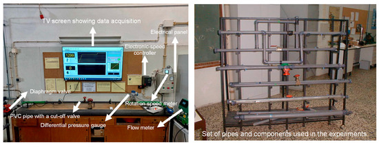
Figure 1.
Experimental setup of ISEC and set of pipes and components used in the experiments.
In the case of major head losses, the main goal is to obtain the exponent of the power equation that characterises the friction losses in a given pipe. In other words, the exponent of the power equation is linked to the roughness of the pipe, increasing as ε increases. The typical form of this equation is
According to Reynolds’ second experiment, that exponent typically ranges between 1.7 and 2.0. As shown in the Darcy–Weisbach, Hazen–Williams, and Flamant equations, the exponent (“b” value) is equal to 2.0, 1.85, and 1.75, respectively. In the Hydraulic Machines Laboratory, galvanised steel, copper, stainless steel, and PVC were available for testing. Figure 2 shows a sample of the experimental results obtained in the laboratory, and Table 2 lists some details of the pipes used in the experiments.
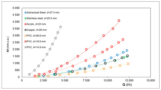
Figure 2.
Experimental results of major losses.
Table 2.
Details of the pipes used in the experiments.
Moreover, in the case of components, tests were also carried out to assess minor losses. Several components were available for testing, namely different types of isolating valves (e.g., cut-off and sphere), regulating valves (e.g., diaphragm and butterfly), one-way valves (e.g., foot valve), elbows (90°) with “tee” lines and branch flows, and filters. Figure 3 shows an example of the evolution of the KL value with a flow test involving four 90° elbows, and Figure 4 highlights the significant difference between the losses in the pipe itself and in the pipe with the four elbows. Table 3 shows a sample of reference KL values derived from the experimental tests in the laboratory.
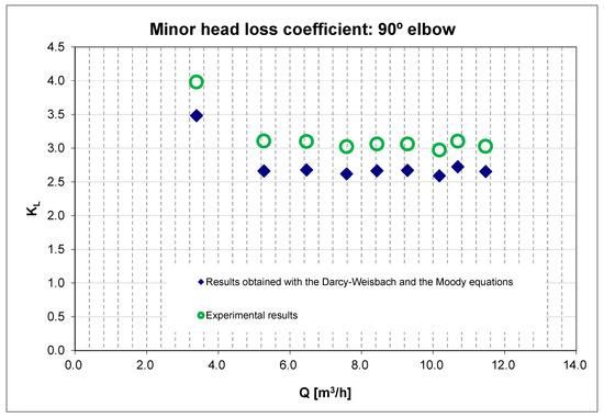
Figure 3.
Evolution of the KL value (four 90° elbows).
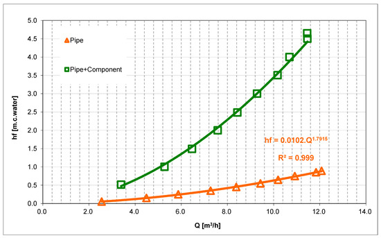
Figure 4.
Major losses in a pipe and in a pipe with four 90° elbows.
Table 3.
Reference KL values derived from the experimental tests.
In the literature, one can find detailed studies for specific components. For instance, Kang et al. [31] evaluated the flow characteristics and the cavitation phenomenon of ball valves using a computational fluid dynamics analysis.
There is a specific worksheet entitled “6_Coef._KL” where the user has access to the KL values of the most common components of a hydraulic installation, namely valves (globe, sphere, etc.), 90° elbows, entrance and exit of tanks, “tee” line and branch flows, foot valves, filters, and sudden contractions. In addition, the user can add a specific component and specify its KL value. A default KL value is suggested for each component, but the user can change this option and choose another considered more appropriate; for instance, for a 90° elbow, the default value is 0.9 but the options 0.85, 0.80, 0.75, and 0.70 are also available. For this purpose, Excel drop-down lists are provided for the different components. Table 4 shows the KL values available for several components: these KL values, shown in worksheet “6_Coef. KL”, are based on the experimental assessments carried out at the Hydraulic Machines Laboratory. For each section of the installation (suction and discharges), the user only has to select which components are present and how many of each. The sum is then performed automatically. Moreover, the user can add more components if necessary. The ones defined correspond to the most typical and are shown for guidance.
Table 4.
KL values available for a set of components.
In the case of major losses, all the details and calculations are performed and presented in the worksheet entitled “10_Head Losses”. However, for the Flamant and Hazen–Williams head loss estimations, the selection of the material is performed in separate worksheets, entitled “8_Material_Flamant” and “9_Material_Hazen-Williams”, respectively. The user only has to select, for each section of the installation, the correct material. The respective coefficients are then automatically considered in the major loss calculation. All these results are presented in the worksheet entitled “10_Head Losses”. The major head losses estimated by the Darcy–Weisbach equation and the friction coefficient estimated by the Moody equation are considered for reference. Finally, the total head losses are estimated by
where ΣK is the sum of the loss coefficients of the additional components (“minor” head losses).
Additionally, the workbook includes a worksheet titled “Head Losses—Leq”, which enables users to compare the total head losses calculated using two different approaches. The first is the reference method, which considers the specific KL values assigned to each component when estimating minor losses. The second is a simplified method, where minor losses are approximated by increasing the total pipe length by 10%, 20%, or 30%, depending on the assumed contribution of fittings. This equivalent length approach is commonly used in engineering practice due to its simplicity and speed, despite its lower accuracy. Therefore, engineers have a wide range of options to perform the calculations, each yielding a different result. With the help of this worksheet, an engineer can gain experience and develop sensitivity to the meaning of the head loss results and then decide on a sound basis which percentage of pipe length is more appropriate for the installation under analysis. Furthermore, when validated with measurements in a given installation, this procedure of comparing results from different calculations allows more accurate assessments and better judgements in the design and dimensioning of future projects.
3.2. System Curve
The system curve of a given installation is obtained by
where Hi is the head rise (system installation) [m], H0 is the height coefficient (geometric difference plus pressure difference between reservoirs), and K′ is the global coefficient of head losses as a function of the flowrate.
The K′ coefficient, for circular pipes, is given by
and KT is obtained by
where KT is the global coefficient of head losses as a function of the fluid velocity.
Although different methodologies are available to perform the calculation of the system curve, a reference method is proposed in the worksheet “7_System curve”. However, because the workbook also offers other options, namely in worksheets “8_Material_Flamant” to “11_Head losses-Leq”, the user might easily evaluate different scenarios. It is important to emphasise that, in the default system curve, KT is obtained on the basis of the friction coefficient λ calculated with the Moody equation. The major losses are calculated with the Darcy-Weisbach equation, and the minor head loss coefficient KL of each component is based on a fixed value presented in the respective worksheet (“6_Coef._KL”).
3.3. Pump Performance Curves
Once the equation of the system curve is known, the head rise (or manometric head, H) for the required flowrate can be calculated. This pair of values (H-Q) allows, by consulting the selection diagram of the suitable type of pump, a first selection of a couple of models. The next step consists of analysing the performance curves of each of the selected models. For each model, the user must carefully read the pump information (characteristic H-Q, efficiency, power, and NPSH curves) provided graphically by the manufacturer and then select a few reference points (we recommend at least 10 points) to enter in the respective worksheet (“4_Pump curve”). This procedure must be performed for each curve (H-Q, P, η and NPSH curves), and the data will then be used is several worksheets, namely “12_Pump selection”, “13_Operationg point (1)”, “14_Efficiency, point 1”, “15_Power, point 1”, and “16_NPSH, point 1”. After this step, there is no more need to consult the manufacturer’s data, as all subsequent analysis is performed within the workbook. To improve accuracy in the graphical reading of the manufacturer data, special attention is required, as this will influence all subsequent analyses and calculations.
3.4. Operating Points
The assessment of the operating point is an important phase in the analysis of a pumping system. For this purpose, four worksheets are used: “13_Operating point (1)”, “14_Efficiency, point 1”, “15_Power, point 1”, and “16_NPSH, point 1” (see Figure 5). The process begins in worksheet 13, where the flowrate is obtained through graphical interpretation, and the corresponding head rise is calculated using the system curve defined in Worksheet 7. The pump’s rotation speed is then set according to the manufacturer’s specifications. Worksheet 14 allows the estimation of the efficiency based on a graphical reading, which in turn is used in Worksheet 13 to compute the power consumption. This value is then cross-checked with the power derived from manufacturer data in Worksheet 15. Such comparisons, also applicable to the head rise, enable users to validate their input and detect inaccuracies caused by poor graphical interpretation. Finally, the Net Positive Suction Head (NPSH) value used in Worksheet 13 is obtained in Worksheet 16, completing the characterisation of the first operating point (Q, H, P, N, η, and NPSH).
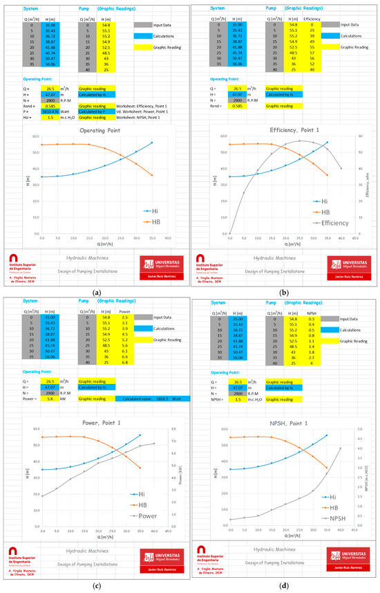
Figure 5.
Procedure to determine the specific characteristics (Q, H, N, η, P, and NPSH) of Point 1: (a) flow (Q) and head rise (H); (b) efficiency (η); (c) power (P); (d) Net Positive Suction Head (NPSH).
Figure 5a shows that the graphical reading of the flow is equal to 26.5 m3/h; this value then allows the calculation of the head rise based on Equation (13) (47.07 m). The rotation speed of the pump is obtained from the manufacturer’s datasheet (2900 rpm). Figure 5b depicts the graphical reading of the efficiency (η = 0.585). With this value, the power consumption is calculated (≅5810.5 W). The result can then be compared with the power graphical reading shown Figure 5c. One can conclude that the calculated values match those obtained from the graphical readings. Finally, Figure 5d shows the graphical reading of the NPSH value (1.5 m.c.H2O).
3.5. Dimensionless Coefficients
Dimensionless coefficients (DCs) can be used for different purposes. In the present context, they are applied to relate operating points that lie on the same Parabola of Equivalent Points (PEP)—a curve that represents geometrically and dynamically similar conditions at different rotation speeds. This analysis is necessary to calculate the rotation speed of the pump for a new required operating point, referred to as “Point 2” here, which represents a new operating condition, different from that obtained when the pump is first placed in the installation (point 1). The PEP determined on the basis of point 2 is obtained by
Hence, any two points that satisfy Equation (16) allow the use of DCs. For the present analysis, four DCs are used: the flow, head rise, power, and Thoma coefficients. They are calculated as follows:
Typically, three operating points are considered, as shown in Figure 6. Point 1 represents the initial condition, obtained when the pump is placed in the installation at the reference rotation speed indicated by the manufacturer (intersection of blue and orange curves). Point 2 represents the new required condition, at a different rotation speed, to be determined (intersection of blue and grey curves). Point 3 (intersection of orange and grey curves) corresponds to the condition obtained in the reference performance curve of the manufacturer but belonging to the same PEP determined on the basis of point 2 (Equation (16)). The PEP and the characteristics of Point 3 are determined in worksheet “17_PEP & Point 3”, and the conditions of point 2, obtained with the DCs, are calculated in worksheet “18_Point 2”.
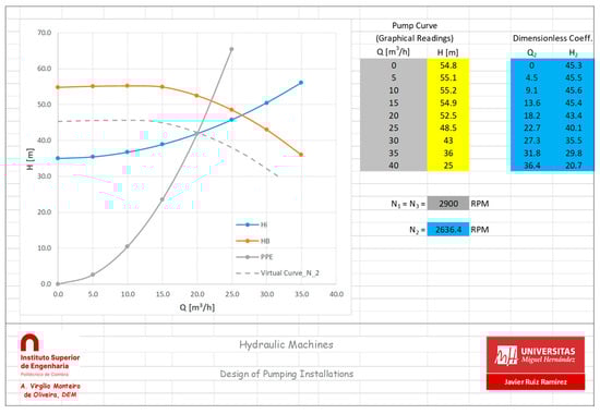
Figure 6.
Operating Points 1, 2, and 3.
This analysis allows the user to accurately define a new operating condition for the pump. By analysing both the power consumption and efficiency of this new operating point, the user might test different options to determine the best solution.
3.6. Net Positive Suction Head (NPSH)
The cavitation phenomenon represents a critical condition in pump operation that must always be avoided and is addressed is two worksheets. Worksheet “19_Pv and Pa” is dedicated to selecting the fluid temperature and the corresponding vapour pressure value and defining the atmospheric pressure at the pump location. In worksheet “20_Cavitation”, the cavitation phenomenon is analysed in detail. Pressure values are shown in three different units (Pascal, m.c.H2O, and mm.c.Hg), and water temperature values are shown in Celsius and Kelvin. Whenever the Net Positive Suction Head (NPSH) required by the pump, as specified by the manufacturer for each specific pump, is lower than the NPSH available in the installation (NPSHrequired < NPSHavailable), there is no cavitation. Therefore, these two values are compared in worksheet “20_Cavitation”. NPSHavailable is calculated by
where Pa is the atmospheric pressure [Pa], γ is the specific weight [N/m3], es is the height of the pump in the installation [m], ΔHsuction is the head losses in the suction pipe of the pump [m.c.H2O], and Pv is the fluid vapour pressure [Pa].
For a given operating condition (Point 1, 2, or 3), the atmospheric and vapour pressures defined in worksheet “19_Pv and Pa” are taken into account. The user must also specify the value of es, which represents the vertical distance between the reference aspiration level and the pump. In addition, the head loss in the suction section is calculated accordingly. It must be emphasised that the values of the NPSHrequired for Points 1 and 3 are obtained from graphical readings of manufacturer data available in worksheets “16_NPSH, point 1” and “17_PPE & Point 3”. For Point 2, the NPSHrequired is obtained using Equation (20). All the calculations are then performed, and the interpretation of whether the pump is operating under cavitation or not is highlighted. If cavitation occurs, the user can perform several tests to decide on the best approach to avoid it. Often, in real engineering practice a safety coefficient is adopted, namely for es, but that common practice is not followed in the workbook.
3.7. Overall Analysis
The workbook allows a final overall assessment of the pumping system. In worksheet “21_Table 3 points + EUR”, a summary of the three different operating points is shown in a table with the head rise, the flowrate, the rotation speed, the efficiency, the power, and the NPSH values. In particular, attention is given to the power consumption and to the efficiency values. In addition, by specifying the energy price in a given country, city, or location, along with the pump’s number of working hours per day and number of working days per month, one can estimate the possible monthly savings. Ultimately, the goal of a pumping system is to operate with the pump’s best efficiency and lower power consumption, an analysis that can be performed with the present workbook (see Figure 7).
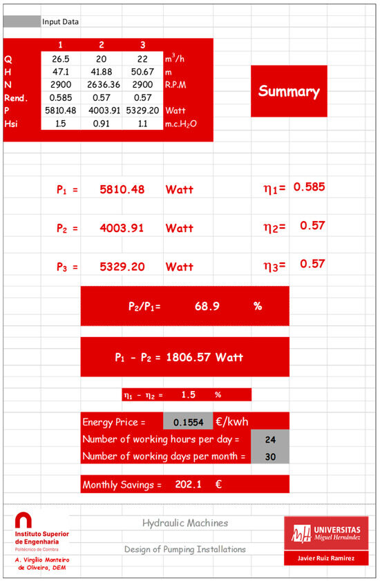
Figure 7.
View of the overall assessment of the pumping system.
Figure 7 shows, in the top left corner, a summary of the three points considered (Q, H, N, η, P, and NPSH). Special attention is paid to the power consumption and efficiency results. At the bottom, an assessment of possible financial savings is presented. This is a specific analysis, as it depends on the corresponding energy price and on the explicit pump’s working hours per day and number of working days per month. Thus, the present worksheet allows the user to easily perform several tests in order to achieve the most efficient and cost-effective solution.
4. Conclusions
The “EEP: Energy-Efficient Pumps Design Tool” Excel workbook represents a contribution intended for use by project engineers and academic staff whenever an energy-efficient pumping system is planned. This work started at the Coimbra Institute of Engineering to address specific goals in Hydraulic Machines lectures of the Mechanical Engineering Degree at ISEC. Following an Erasmus Mobility at Miguel Hernández University of Elche (UMH) in Spain, the initial objectives were expanded to meet specific goals of the Fluid Installations lectures in the master’s programme in HVAC and Electrical Facilities, Energy Efficiency at UMH. The first draft of this work was presented at CYTEF Conference 2024 [10]. The workbook includes several features, namely, a comparison of equations for estimating head losses in pipes (major losses); a comparison of explicit and implicit equations for estimating the friction coefficient (λ); a procedure to obtain the system equation of a given installation; a procedure to calculate the rotation speed of the pump to obtain a specific operating point; and a procedure to assess the occurrence of cavitation, among others. Some limitations must be underlined, namely with regard to the calculations of the major head losses (only the Darcy–Weisbach, Hazen–Williams, and Flamant equations are used), the friction coefficient (estimated with explicit (Haaland, J.J. Chen, and Moody) and implicit (Colebrook) equations), and the minor head losses, determined on the basis of the KL value. The assessment of head losses is a critical aspect in every pumping system, since the power required for transporting a given fluid between two points is directly related to this factor. This justifies the special attention given to the topic in the workbook. It should also be mentioned that the system curve is determined considering one suction section and two discharge sections. Despite these limitations, which can all be easily overcome by implementing the necessary changes in Excel, the workbook enables an overall assessment of a pumping system according to the user’s specific goals and supports the design of sustainable pumping systems.
Finally, the authors would like to emphasise the nature of the present contribution, which embodies the spirit of the ERASMUS programme within the European Union. Following the first Erasmus Mobility, the idea of designing a tool for use at both ISEC-Portugal and UMH-Spain began to take shape. At its current stage of development, the “EEP Design Tool” already fulfils its initial objectives, although further development is clearly encouraged to address additional and complementary objectives. For instance, enhancing existing features and introducing more interactive or alternative tools for pump system design are welcome directions. Moreover, the authors hope this contribution will help strengthen the ongoing cooperation between the two institutions involved.
Supplementary Materials
The following supporting information can be downloaded at: https://www.mdpi.com/article/10.3390/en18164248/s1, File S1: EEP workbook; File S2: example of a problem statement.
Author Contributions
All authors contributed to the study conception and design. Material preparation, data collection, and analysis were performed by A.V.M.O. and J.R.R. The first draft of the manuscript was written by A.V.M.O., and both authors commented on previous versions of the manuscript. All authors have read and agreed to the published version of the manuscript.
Funding
This research received no external funding.
Data Availability Statement
All datasets used in this analysis are available.
Acknowledgments
The authors would like to acknowledge João Ferreira Mendes for the design and development of the experimental setup at the Coimbra Institute of Engineering.
Conflicts of Interest
The authors declare no conflicts of interest.
References
- Ribeiro, J.T.G. Sistemas Elevatórios de Águas Residuais em Edifícios. Dissertação de Mestrado em Engenharia Civil, Especialização em Construções. Master’s Thesis, Faculdade de Engenharia da Universidade do Porto, Porto, Portugal, 2014. (In Portuguese). [Google Scholar]
- Grundfos. Seminário Gestão Eficiente de Bombas Centrífugas; Instituto Superior de Engenharia de Coimbra: Coimbra, Portugal, 2024. (In Portuguese) [Google Scholar]
- Grundfos. Grunfdos Product Selection. 2025. Available online: https://product-selection.grundfos.com/pt/advanced-selection (accessed on 30 July 2025).
- Zhang, H.; Li, K.; Liu, T.; Liu, Y.; Hu, J.; Zuo, Q.; Jiang, L. Analysis the Composition of Hydraulic Radial Force on Centrifugal Pump Impeller: A Data-Centric Approach Based on CFD Datasets. Appl. Sci. 2025, 15, 7597. [Google Scholar] [CrossRef]
- Nan, L.; Wang, Y.; Chen, D.; Huang, W.; Zhu, Z.; Liu, F. A Novel Energy Performance Prediction Approach towards Parametric Modeling of a Centrifugal Pump in the Design Process. Water 2023, 15, 1951. [Google Scholar] [CrossRef]
- Pei, Y.; Liu, Q.; Ooi, K.T. Research on Energy-Efficient Disc Pumps: A Review on Physical Models and Energy Efficiency. Machines 2023, 11, 954. [Google Scholar] [CrossRef]
- Yu, J.; Akoto, E.; Degbedzui, D.K.; Hu, L. Predicting Centrifugal Pumps’ Complete Characteristics Using Machine Learning. Processes 2023, 11, 524. [Google Scholar] [CrossRef]
- Pavlenko, I.; Kulikov, O.; Ratushnyi, O.; Ivanov, V.; Pitel’, J.; Kondus, V. Effect of Impeller Trimming on the Energy Efficiency of the Counter-Rotating Pumping Stage. Appl. Sci. 2023, 13, 761. [Google Scholar] [CrossRef]
- Pavlenko, I.; Ciszak, O.; Kondus, V.; Ratushnyi, O.; Ivchenko, O.; Kolisnichenko, E.; Kulikov, O.; Ivanov, V. An Increase in the Energy Efficiency of a New Design of Pumps for Nuclear Power Plants. Energies 2023, 16, 2929. [Google Scholar] [CrossRef]
- Oliveira, A.V.M.; Ramirez, J.R.; Mendes, J.C.A.F. Design of Pumping Installations: Development of an Excel Workbook for Hydraulic Machines Lectures. In Proceedings of the CYTEF 2024—XII Iberian Congress/X Ibero-American Congress Refrigeration Sciences and Technologies, Elche, Spain, 26–28 June 2024; Valero, F.J.A., García, S.C., Llorens, D.C., Miralles, M.L., Beltrán, P.J.M., Martínez, P.M., González, J.M., Cámara, J.M., Ramírez, J.R., Quiles, P.G.V., Eds.; (Abstract Book). p. 96, ISBN 978-84-09-61977-1. [Google Scholar] [CrossRef]
- Lahiouel, Y.; Lahiouel, R. Evaluation of energy losses in pipes. In Proceedings of the CFM2015-22ème, Congrès Français de Mécanique, Lyon, France, 24–28 August 2015. [Google Scholar]
- Prates Coelho, A.; Renato Zanini, J.; Teixeira de Faria, R.; Barcellos Dalri, A.; Fabiano Palaretti, L. Comparação de equações para estimativa da perda de carga em tubulações de polietileno. Appl. Res. Agrotechnol. 2018, 11, 25–31. (In Portuguese) [Google Scholar]
- Vidal, L.E.O.; Maury, D.E.C.; Chipana, R.A.F. Hydraulic balance of mine pumping systems: A case study. Ingeniare Rev. Chil. Ing. 2010, 18, 335–342. [Google Scholar]
- Madodi, S.A.; Abdul Wahhab, H.A.; Mahmoud, N.S. Comparative Assessment of Friction Head Losses in Pipe Flow. In ICPER 2020. Lecture Notes in Mechanical Engineering 2023; Ahmad, F., Al-Kayiem, H.H., King Soon, W.P., Eds.; Springer: Singapore, 2022. [Google Scholar] [CrossRef]
- Robaina, A.D. Análise de equações explícitas para o cálculo do coeficiente “f” da fórmula universal de perda de carga. Ciência Rural. Santa Maria 1992, 22, 157–159. (In Portuguese) [Google Scholar] [CrossRef]
- Marques, J.A.A.S.; Sousa, J.J.O. Fórmula de Colebrook-White: Velha mas actual. Soluções empíricas. Faculdade de Ciências e Tecnologia da Universidade de Coimbra. In Proceedings of the Atas do III SILUSBA—Simpósio de Hidráulica e Recursos Hídricos dos Países de Língua Oficial Portuguesa, Maputo, Moçambique, 15–19 April 1997. (In Portuguese). [Google Scholar]
- Sousa, J.J.O.; Cunha, M.C.; Marques, J.A.A.S. An explicit solution to the Colebrook-White equation through Simulated Annealing. In Water Industry Systems: Modelling and Optimization Applications; Savic, D., Walters, G., Eds.; Research Studies Press LTD: Boston, MA, USA, 1999; pp. 347–355. ISBN 0863802486/978-0863802485. [Google Scholar]
- Araújo, R.S.; Bezerra, A.A.; Sousa, M.C.B.; Moura, B.D. Influência das equações explícitas de fator de atrito no dimensionamento de redes de distribuição. In Proceedings of the 30° Congresso Brasileiro de Engenharia Sanitária e Ambiental (ABES-2019), Natal, Brazil, 16–19 June 2019. (In Portuguese). [Google Scholar]
- Muzzo, L.E.; Matoba, G.K.; Ribeiro, L.F. Uncertainty of pipe flow friction factor equations. Mech. Res. Commun. 2021, 116, 103764. [Google Scholar] [CrossRef]
- Young, F.Y.; Munson, B.R.; Okiishi, T.H.; Huebsch, W.W. Introduction to Fluid Mechanics, 5th ed.; John Wiley & Sons, Inc.: Hoboken, NJ, USA, 2012; ISBN 978-0-470-90215-8. [Google Scholar]
- Hazen, A. Storage to be provided in impounding reservoirs for municipal water supply. Trans. Am. Soc. Civ. Eng. 1914, 77, 1539–1640. [Google Scholar] [CrossRef]
- Flamant, A. Sur la répartition des pressions dans un solide rectangulaire chargé transversalement. CR Acad. Sci. 1892, 114, 1465–1468. [Google Scholar]
- Moody, L.F. An approximate formula for pipe friction factors. Trans. Am. Soc. Mech. Eng. 1947, 69, 1005–1011. [Google Scholar]
- Haaland, S.E. Simple and explicit formulas for the friction factor in turbulent pipe flow. J. Fluids Eng. 1983, 105, 89–90. [Google Scholar] [CrossRef]
- Chen, J.J. A simple explicit formula for the estimation of pipe friction factor. Proc. Inst. Civ. Eng. 1984, 77 Pt 2, 49–55. [Google Scholar] [CrossRef]
- Colebrook, C.F. Turbulent flow in pipes, with particular reference to the transition region between the smooth and rough pipe laws. J. Inst. Civ. Eng. 1939, 11, 133–156. [Google Scholar] [CrossRef]
- Muzzo, L.E.; Pinho, D.; Lima, L.E.M.; Ribeiro, L.F. Accuracy/speed analysis of pipe friction factor correlations. In INCREaSE 2019 Proceedings of the 2nd International Congress on Engineering and Sustainability in the XXI Century; Springer Nature Switzerland AG: Cham, Switzerland, 2019; pp. 664–679. [Google Scholar]
- Moody, L.F. Friction factors for pipe flow. Trans. ASME 1944, 66, 671–684. [Google Scholar] [CrossRef]
- Colebrook, C.F.; White, C.M. Experiments with fluid friction in roughened pipes. Proc. R. Soc. A 1937, 161, 367–381. [Google Scholar]
- Bistafa, S. Mecânica dos Fluidos: Noções e Aplicações; Editora Blucher: São Paulo, Brazil, 2010; ISBN 978-85-212-0497-8. (In Portuguese) [Google Scholar]
- Kang, H.L.; Park, H.J.; Han, S.H. Investigation of the Flow Characteristics for Cylinder-in-Ball Valve Due to a Change in the Opening Rate. Appl. Sci. 2022, 12, 8930. [Google Scholar] [CrossRef]
Disclaimer/Publisher’s Note: The statements, opinions and data contained in all publications are solely those of the individual author(s) and contributor(s) and not of MDPI and/or the editor(s). MDPI and/or the editor(s) disclaim responsibility for any injury to people or property resulting from any ideas, methods, instructions or products referred to in the content. |
© 2025 by the authors. Licensee MDPI, Basel, Switzerland. This article is an open access article distributed under the terms and conditions of the Creative Commons Attribution (CC BY) license (https://creativecommons.org/licenses/by/4.0/).