
Construction of Analogy Indicator System and Machine-Learning-Based Optimization of Analogy Methods for Oilfield Development Projects

Abstract
1. Introduction
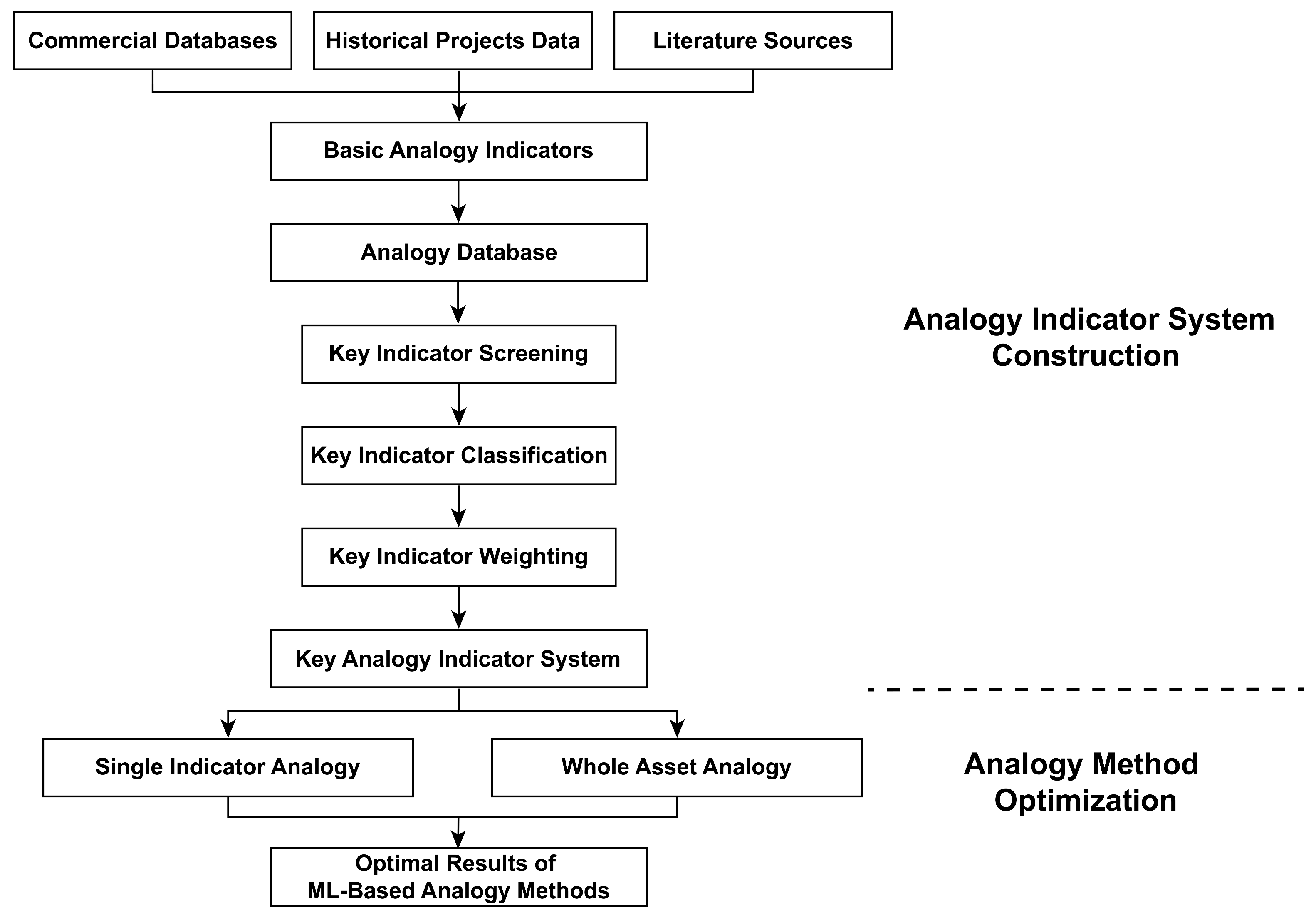
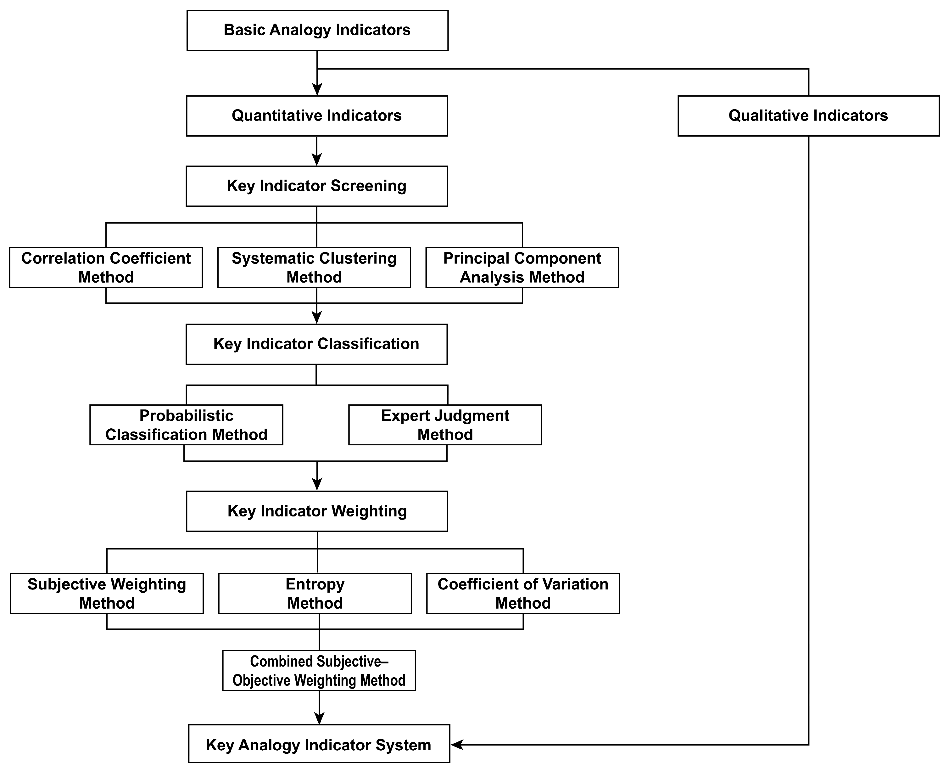
- A range of statistical techniques, including the correlation coefficient, systematic clustering, and principal component analysis, are used to screen the original set of indicators and identify key analogy indicators. A classification scheme is then created for the selected key indicators based on probability statistics analysis and expert judgment, ensuring both representativeness and engineering relevance.
- A combined subjective–objective weighting method is proposed for key indicators. Subjective weights are assigned using direct expert scoring, while objective weights are derived from the averaged results of the entropy method and the coefficient of variation method. This approach ensures that the weighting reflects both expert experience and data characteristics.
- Through screening, classification, and weighting, a comprehensive analogy indicator system is developed. It combines static and dynamic parameters from geological, petrophysical, and development aspects, integrating both subjective and objective views to support similarity evaluation between target and candidate oilfields.
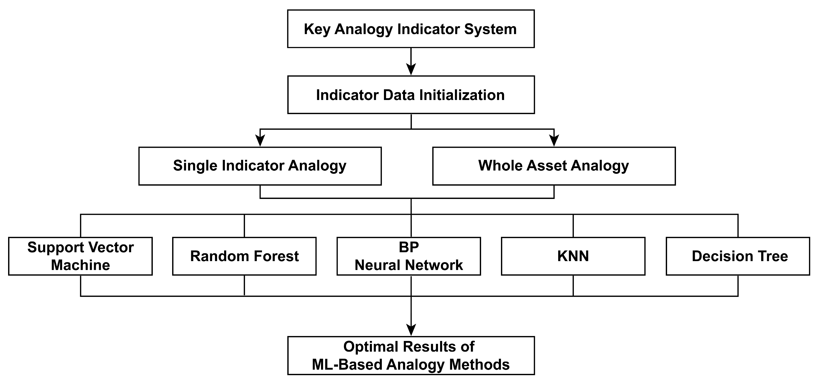
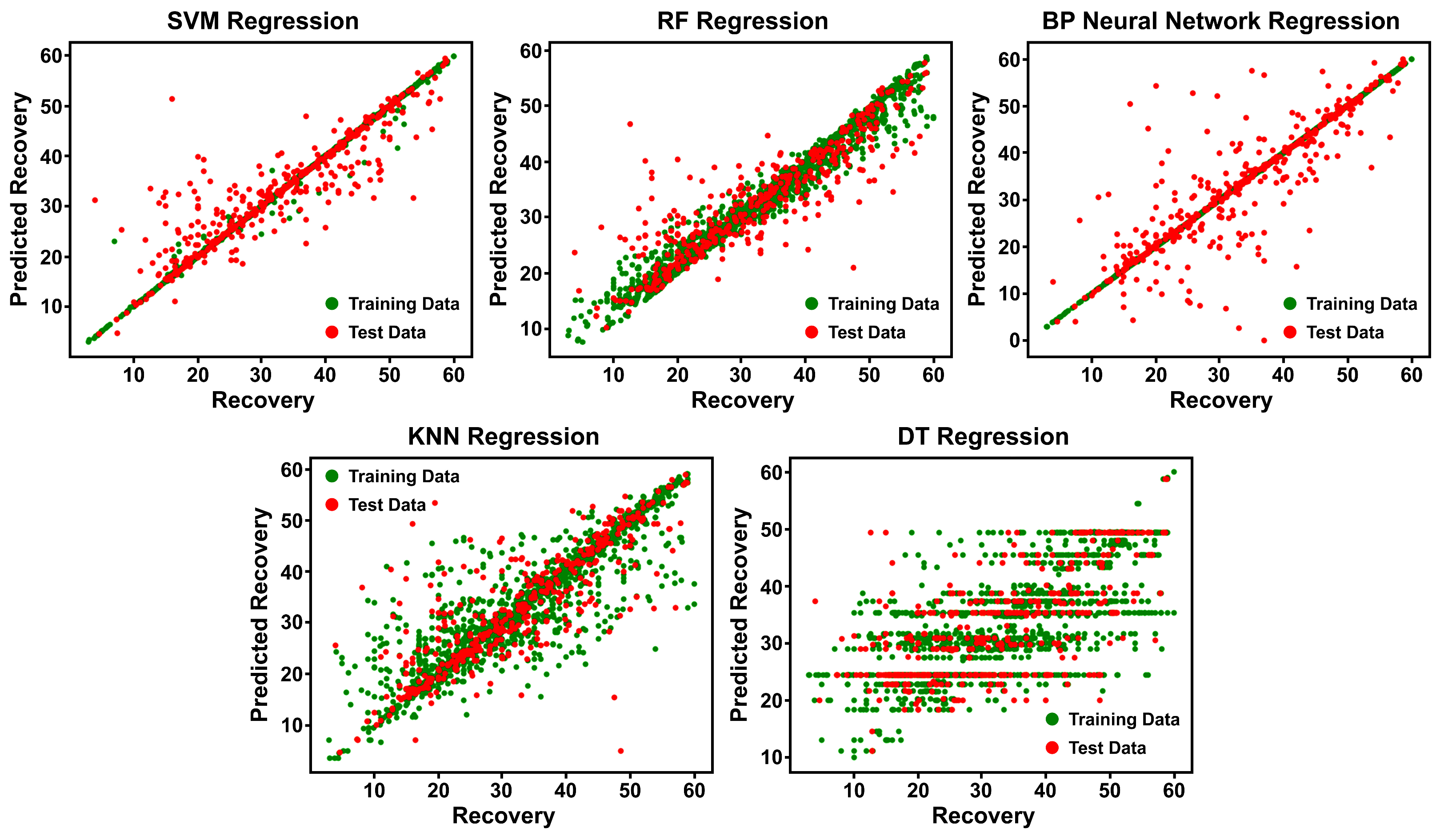
- Five machine-learning methods—support vector machine (SVM), random forest (RF), backpropagation neural network (BP), k-nearest neighbor (KNN), and decision tree (DT)—are used to perform both single indicator and whole analogy experiments. The adaptability and prediction accuracy of each method are evaluated under different reservoir conditions, such as medium-to-high permeability sandstone and low-permeability sandstone, leading to the identification of the optimal algorithm.
2. Materials and Methods
2.1. Analogy Indicator System for Oilfield Development Projects
2.1.1. Key Indicator Screening
Correlation Coefficient Method
Systematic Clustering Method
- Each sample or variable is initially treated as an independent class, denoted as G1, G2, …, Gₙ. All pairwise distances are calculated to form the initial distance matrix D(0), where the element Dij = dxy represents the distance between variables.
- The minimum distance element in the current matrix is selected as Dpq = min {Dij}, and the corresponding classes Gp and Gq are merged to form a new class Gs.
- The distance matrix is updated by calculating the distance between the new class Gs and any other class Gk as Dsk = min {Dpk, Dqk}, where Dpk and Dqk are the distances between the original classes Gp, Gq, and class Gk.
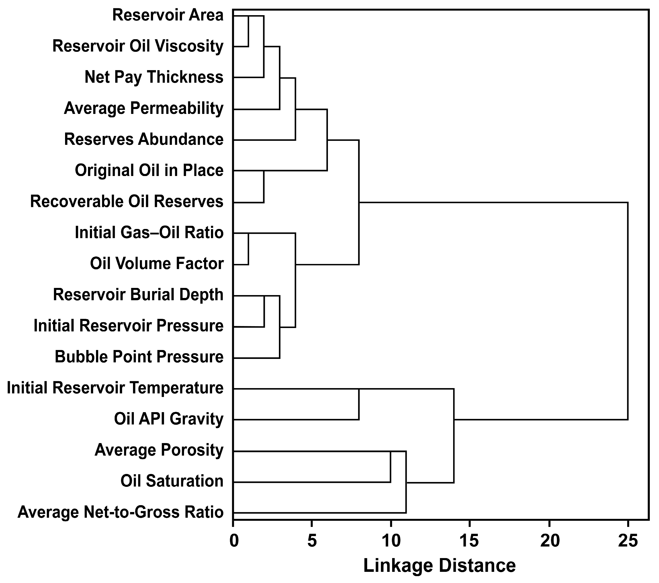
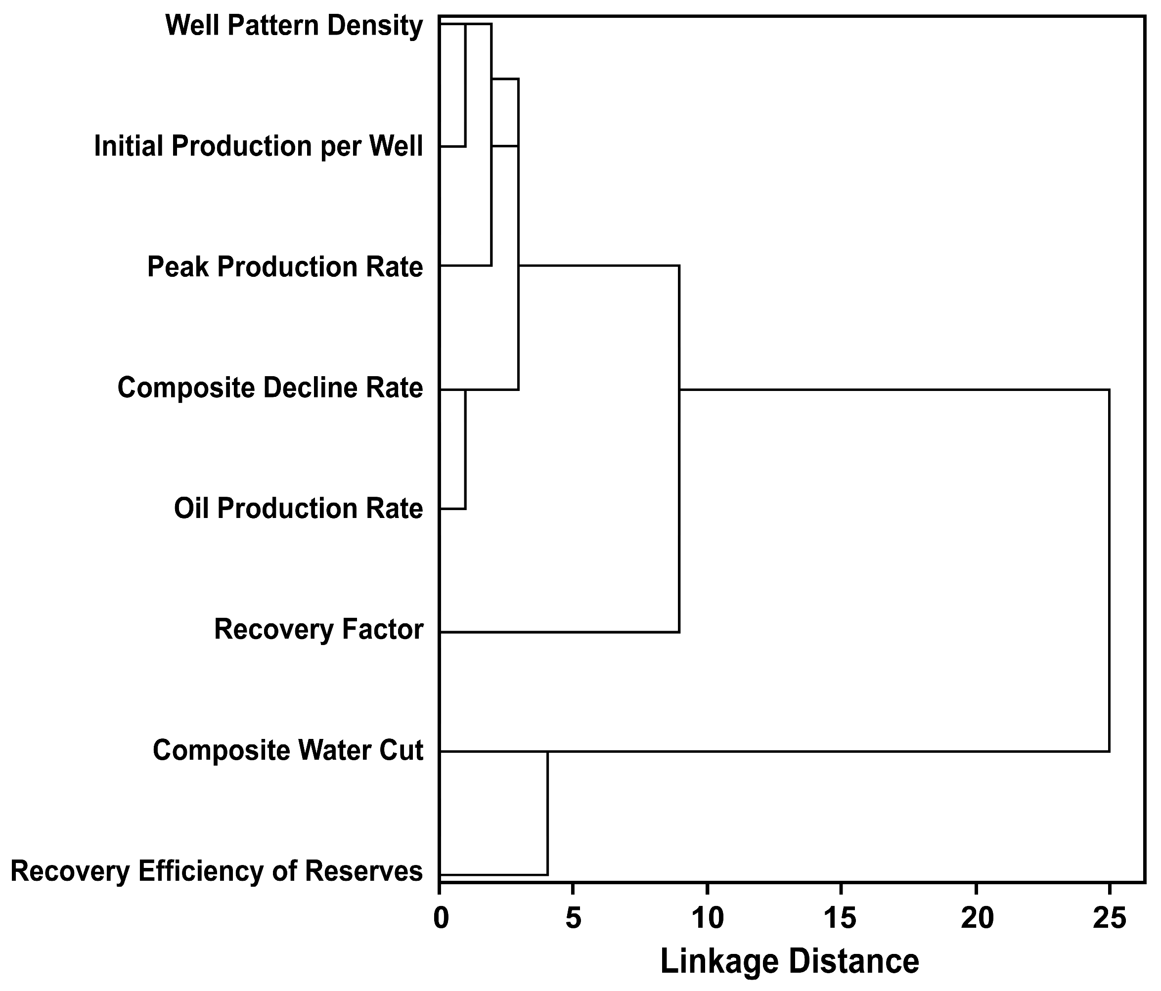
- The above steps are repeated until all classes are merged into a single class. The entire clustering process can be visualized using a dendrogram, and researchers can determine the final classification scheme by selecting an appropriate distance threshold based on practical needs.
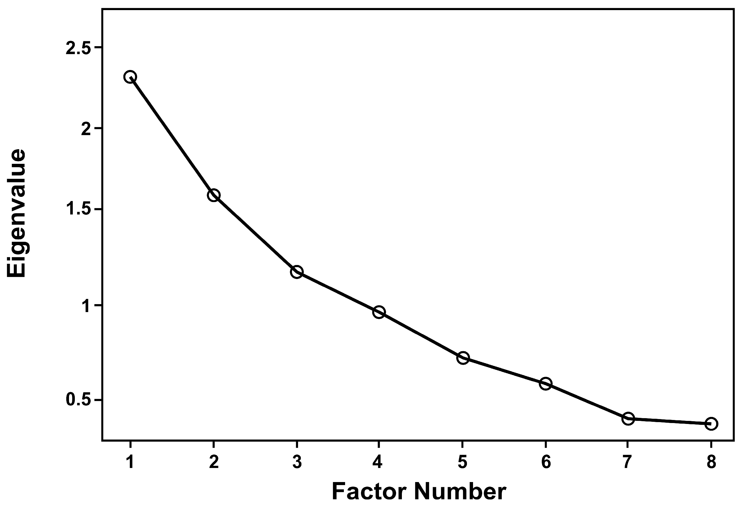
Principal Component Analysis Method
- Standardize the original variables to zero mean and unit variance in order to eliminate the influence of differing units and scales.
- Construct the correlation matrix R for the original variables.
- Perform eigenvalue decomposition on the correlation matrix R. Let be the matrix composed of the top principal eigenvectors, and be the diagonal matrix of the corresponding eigenvalues. The factor loading matrix can then be computed as:
- 4.
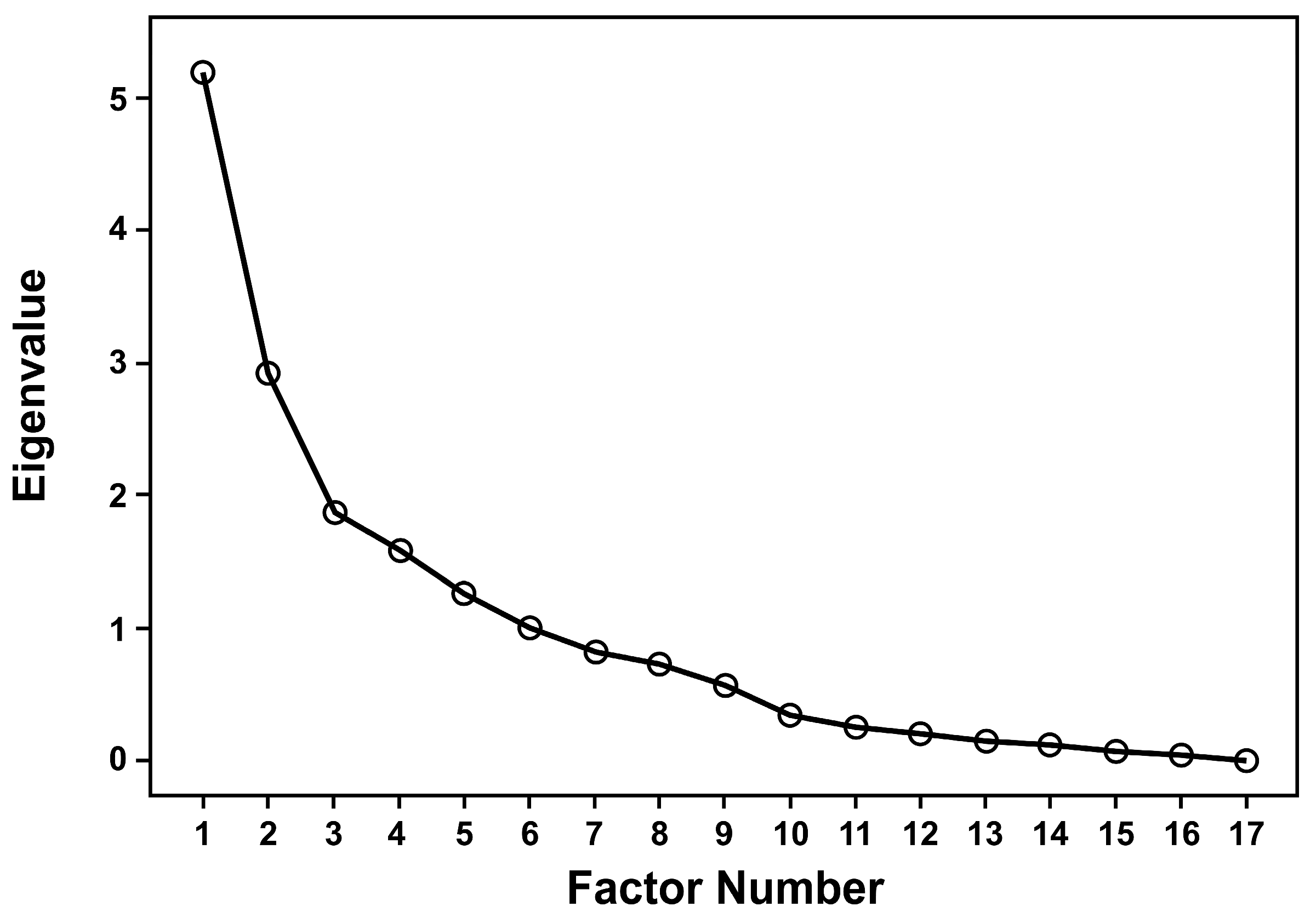
- Determine the number of factors k based on the cumulative variance contribution rate, choosing the smallest k such that the cumulative explained variance is at least 90%.
- 5.
- Linearly transform the original variables into factor scores to be used as inputs for subsequent modeling. Let wⱼᵢ denote the weight of variable Xᵢ on factor Fⱼ, and the factor score, which is a weighted sum of all variables on a given factor, can be calculated as follows:
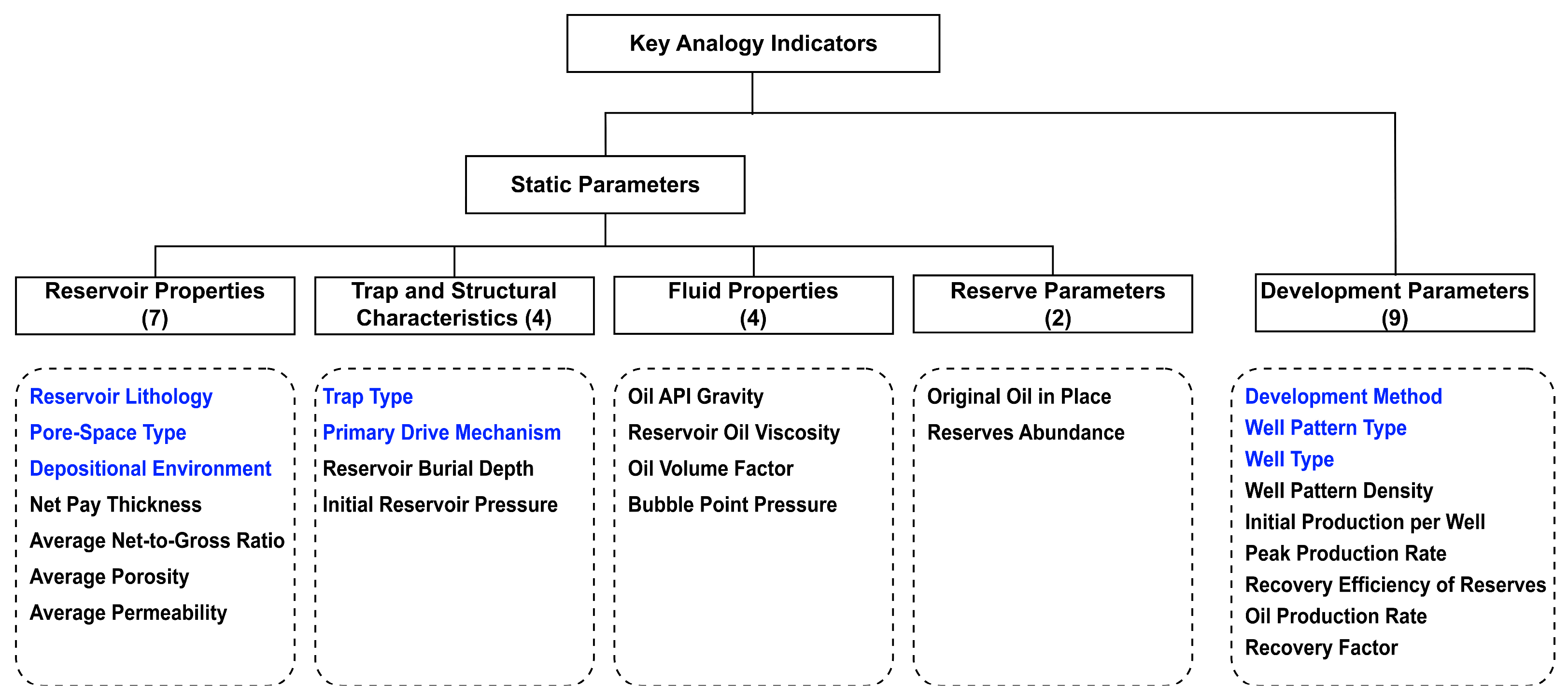
2.1.2. Key Indicators Classification
- 1.
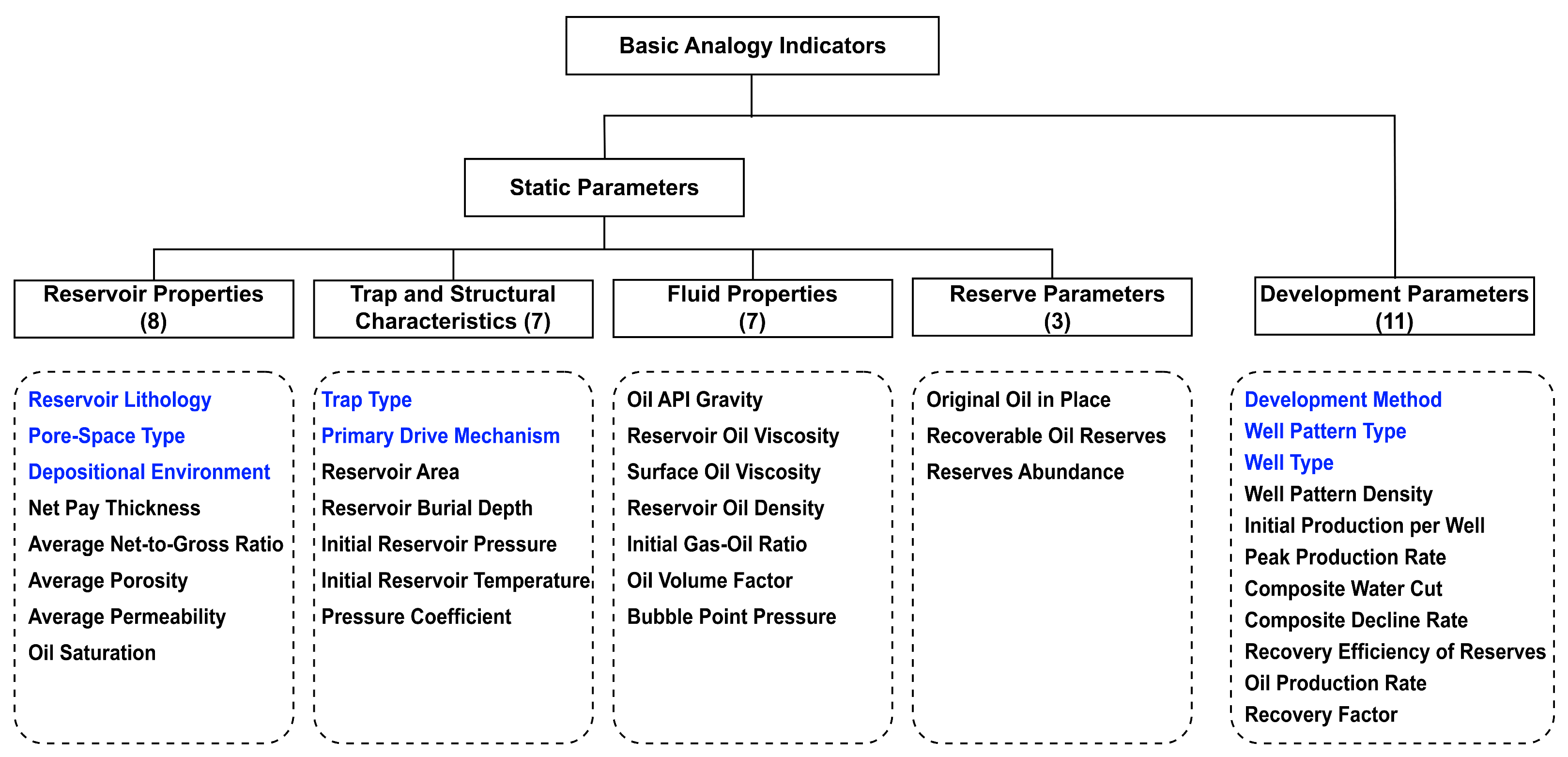
- Normal distribution type: This includes indicators such as Average Porosity, Reservoir Burial Depth, Initial Reservoir Pressure, Oil API Gravity, Original Oil in Place, and Recovery Factor.For normally distributed indicators, the classification thresholds were calculated based on the mean () and standard deviation (), using the values: .
- 2.
- Exponential distribution type: This category includes Net Pay Thickness, Average Permeability, Oil Volume Factor, Bubble Point Pressure, Reserves Abundance, Well Pattern Density, Initial Production per Well, Peak Production Rate, and Oil Production Rate.For exponentially distributed indicators, the classification thresholds were determined based on the characteristic quantiles extracted from the cumulative distribution function (CDF) at probability levels of 15%, 30%, 70%, and 85%.
- 3.
- Uniform distribution type: This category includes Average Net-to-Gross Ratio and Recovery Efficiency of Reserves.For uniformly distributed indicators, the classification thresholds were defined by the characteristic quantiles extracted from the CDF at probability levels of 20%, 40%, 60%, and 80%.
2.1.3. Key Indicator Weighting
Entropy Method
- 1.
- Normalize the data. Let denote the sample index and denote the indicator index. Let represent the original value of the -th indicator for the -th sample. Denote the minimum and maximum values of all samples for the -th indicator as and , respectively. Each is linearly mapped to the interval [0, 1], resulting in the normalized value .For a positive indicator, the normalization is computed as follows:For a negative indicator, the normalization is computed as follows:
- 2.
- Calculate the proportion of the -th indicator in the -th sample, denoted as , using the following formula:
- 3.
- Compute the entropy value of the -th indicator. Let be the total number of samples and be the normalization constant. The entropy value is calculated as follows:
- 4.
- Compute the redundancy and derive the weight of each indicator. The redundancy is given by , and the final weight is calculated as follows:
Coefficient of Variation Method
Combined Subjective–Objective Weighting Method
2.2. Analogy Methods for Oilfield Development Projects
2.2.1. Machine-Learning Methods
2.2.2. Single Indicator Analogy
2.2.3. Whole Asset Analogy
- 1.
- Construct the evaluation matrix by arranging the indicators as columns and the 663 oilfields as rows.
- 2.
- Normalize each indicator to the [0, 1] range and multiply by its obtained key-indicator weight.
- 3.
- Compute each oilfield’s analogy score by summing the weighted, normalized scores.
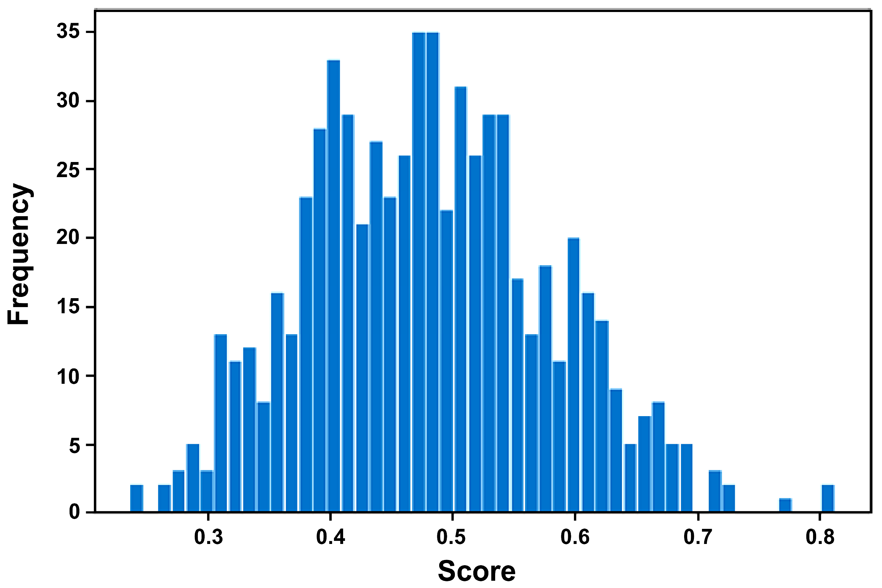
- 4.
- Plot the score histogram and, based on empirical distribution characteristics, divide S into five intervals to define the asset levels.
3. Results and Analysis
3.1. Construction of the Analogy Indicator System
3.1.1. Results of Key Indicator Screening
Correlation Coefficient Method
Systematic Clustering Method
Principal Component Analysis Method
3.1.2. Results of Key Indicators Classification
3.1.3. Results of Key Indicator Weighting
3.2. Analogy Method Optimization
3.2.1. Results of Single Indicator Analogy
3.2.2. Results of Whole Asset Analogy
4. Conclusions
Author Contributions
Funding
Data Availability Statement
Conflicts of Interest
References
- Dong, W.; Jiao, J.; Xie, S.; Lyu, C.; Cui, G.; Meng, J. Cumulative production curve method for the quantitative evaluation on the effect of oilfield development measures: A case study of the nitrogen injection pilot in Yanling oilfield, Bohai Bay Basin. Pet. Explor. Dev. 2016, 43, 672–678. [Google Scholar] [CrossRef]
- Ponomarenko, T.; Marin, E.; Galevskiy, S. Economic Evaluation of Oil and Gas Projects: Justification of Engineering Solutions in the Implementation of Field Development Projects. Energies 2022, 15, 3103. [Google Scholar] [CrossRef]
- Ponomarenko, T.V.; Sergeev, I.B. Valuation of mineral assets of a mining company on the basis of the option approach. J. Min. Inst. 2011, 191, 164–175. [Google Scholar]
- Mu, L.X.; Fan, Z.F.; Xu, A.Z. Development characteristics, models and strategies for overseas oil and gas fields. Pet. Explor. Dev. 2018, 45, 735–744. [Google Scholar] [CrossRef]
- Li, Z.X.; Liu, J.Y.; Luo, D.K.; Wang, J.J. Study of evaluation method for the overseas oil and gas investment based on risk compensation. Pet. Sci. 2020, 17, 858–871. [Google Scholar] [CrossRef]
- Yusgiantoro, P.; Hsiao, F.S.T. Production-sharing contracts and decision-making in oil production: The case of Indonesia. Energy Econ. 1993, 15, 245–256. [Google Scholar] [CrossRef]
- Sidle, R.E.E.; Lee, W.J.J. An Update on the Use of Reservoir Analogs for the Estimation of Oil and Gas Reserves. SPE Econ. Manag. 2010, 2, 80–85. [Google Scholar] [CrossRef]
- Liu, Z.L.; Geng, M.; Zhang, Y.Z. The Method for Selecting Analogous Reservoirs Based on SEC. J. Phys. Conf. Ser. 2023, 2520, 012008. [Google Scholar] [CrossRef]
- Martín Rodríguez, H.; Escobar, E.; Embid, S.; Rodríguez Morillas, N.; Hegazy, M.; Lake, L.W. New Approach to Identify Analogous Reservoirs. SPE Econ. Manag. 2014, 6, 173–184. [Google Scholar] [CrossRef]
- El-Nikhely, A.; El-Gendy, N.H.; Bakr, A.M.; Zawra, M.S.; Ondrak, R.; Barakat, M.K. Decoding of seismic data for complex stratigraphic traps revealing by seismic attributes analogy in Yidma/Alamein concession area Western Desert, Egypt. J. Petrol. Explor. Prod. Technol. 2022, 12, 3325–3338. [Google Scholar] [CrossRef]
- Liu, X.H.; Hu, T.; Pang, X.Q.; Xu, Z.; Wang, T.; Zhang, X.W.; Wang, E.Z.; Wu, Z.Y. Evaluation of natural gas hydrate resources in the South China Sea using a new genetic analogy method. Pet. Sci. 2022, 19, 48–57. [Google Scholar] [CrossRef]
- Awoleke, O.O.; Lane, R.H. Analysis of data from the Barnett Shale using conventional statistical and virtual intelligence techniques. SPE Res. Eval. Eng. 2011, 14, 544–556. [Google Scholar] [CrossRef]
- Iraji, S.; Soltanmohammadi, R.; Matheus, G.F.; Basso, M.; Vidal, A.C. Application of unsupervised learning and deep learning for rock type prediction and petrophysical characterization using multi-scale data. Geoenergy Sci. Eng. 2023, 230, 212241. [Google Scholar] [CrossRef]
- Wang, Y.; Cheng, S.Q.; Zhang, F.B.; Feng, N.C.; Li, L.; Shen, X.Z.; Li, J.H.; Yu, H. Big data technique in the reservoir parameters’ prediction and productivity evaluation: A field case in western South China Sea. Gondwana Res. 2021, 96, 22–36. [Google Scholar] [CrossRef]
- Werneck, R.d.O.; Prates, R.; Moura, R.; Gonçalves, M.M.; Castro, M.; Soriano-Vargas, A.; Mendes Júnior, P.R.; Hossain, M.M.; Zampieri, M.F.; Ferreira, A.F.; et al. Data-driven deep-learning forecasting for oil production and pressure. J. Pet. Sci. Eng. 2022, 210, 109937. [Google Scholar] [CrossRef]
- Zhou, Q.; Dilmore, R.; Kleit, A.; Wang, J.Y. Evaluating gas production performances in Marcellus using data mining technologies. J. Nat. Gas Sci. Eng. 2014, 20, 109–120. [Google Scholar] [CrossRef]
- Yuan, Z.H.; Qin, W.Z.; Zhao, J.S. Smart Manufacturing for the Oil Refining and Petrochemical Industry. Engineering 2017, 3, 179–182. [Google Scholar] [CrossRef]
- Zhang, M.Z.; Jia, A.L.; Lei, Z.X. Inter-well reservoir parameter prediction based on LSTM-Attention network and sedimentary microfacies. Geoenergy Sci. Eng. 2024, 235, 212723. [Google Scholar] [CrossRef]
- Bai, W.P.; Cheng, S.Q.; Guo, X.Y.; Wang, Y.; Guo, Q.; Tan, C.D. Oilfield analogy and productivity prediction based on machine learning: Field cases in PL oilfield, China. Pet. Sci. 2024, 21, 2554–2570. [Google Scholar] [CrossRef]
- Guo, Q.; Cheng, S.Q.; Zeng, F.H.; Wang, Y.; Lu, C.; Tan, C.D.; Li, G.L. Reservoir permeability prediction based on analogy and machine learning methods: Field cases in DLG Block of Jing’an Oilfield, China. Lithosphere 2022, 2022, 5249460. [Google Scholar] [CrossRef]
- Mahdaviara, M.; Sharifi, M.; Ahmadi, M. Toward evaluation and screening of the enhanced oil recovery scenarios for low permeability reservoirs using statistical and machine learning techniques. Fuel 2022, 325, 124795. [Google Scholar] [CrossRef]
- Rahimi, M.; Riahi, M.A. Reservoir facies classification based on random forest and geostatistics methods in an offshore oilfield. J. Appl. Geophys. 2022, 201, 104640. [Google Scholar] [CrossRef]
- Zhang, M.Z.; Jia, A.L.; Lei, Z.X.; Lei, G. A comprehensive asset evaluation method for oil and gas projects. Processes 2023, 11, 2398. [Google Scholar] [CrossRef]
- Kassem, M.A.; Khoiry, M.A.; Hamzah, N. Using Relative Importance Index Method for Developing Risk Map in Oil and Gas Construction Projects. J. Kejuruter. 2020, 32, 441–453. [Google Scholar] [CrossRef]
- Bi, A.; Huang, S.; Sun, X. Risk Assessment of Oil and Gas Pipeline Based on Vague Set-Weighted Set Pair Analysis Method. Mathematics 2023, 11, 349. [Google Scholar] [CrossRef]
- Ni, S.; Tang, Y.; Wang, G.; Yang, L.; Lei, B.; Zhang, Z. Risk identification and quantitative assessment method of offshore platform equipment. Energy Rep. 2022, 8, 7219–7229. [Google Scholar] [CrossRef]
- Rui, Z.; Lu, J.; Zhang, Z.; Guo, R.; Ling, K.; Zhang, R.; Patil, S. A quantitative oil and gas reservoir evaluation system for development. J. Nat. Gas Sci. Eng. 2017, 42, 31–39. [Google Scholar] [CrossRef]
- Vilela, M.; Oluyemi, G.; Petrovski, A. A fuzzy inference system applied to value of information assessment for oil and gas industry. Decis. Mak. Appl. Manag. Eng. 2019, 2, 1–18. [Google Scholar] [CrossRef]
- Ilyushin, Y.; Nosova, V.; Krauze, A. Application of Systems Analysis Methods to Construct a Virtual Model of the Field. Energies 2025, 18, 1012. [Google Scholar] [CrossRef]
- Li, M.; Qu, Z.; Wang, M.; Ran, W. The Influence of Micro-Heterogeneity on Water Injection Development in Low-Permeability Sandstone Oil Reservoirs. Minerals 2023, 13, 1533. [Google Scholar] [CrossRef]


| Method | Advantages | Disadvantages | Applicable Scenarios | Algorithm Principle |
|---|---|---|---|---|
| Support Vector Machine (SVM) | Performs well on high-dimensional, nonlinearly separable data; good generalization. | Lacks interpretability; decision process not intuitive. | Suitable for relatively small samples with high feature dimensionality. | Maps inputs via kernel functions into a high-dimensional space and finds the hyperplane that maximizes class margin. |
| Random Forest (RF) | Strong noise robustness; resistant to overfitting. | High memory footprint; computationally expensive for training and inference. | Works well on high-dimensional or very large datasets. | Ensembles multiple decision trees trained on bootstrapped samples and random feature subsets; predictions by majority vote or averaging. |
| Backpropagation Neural Network (BP) | Flexible architecture; capable of modeling complex nonlinear mappings. | Black-box model; internal workings hard to interpret. | Well suited for large datasets and complex nonlinear tasks. | Multi-layer feedforward network trained by backpropagation using gradient descent to minimize prediction error. |
| K-Nearest Neighbors (KNN) | Simple to implement; intuitive prediction by neighbors. | High storage and computation cost, especially for large datasets. | Suitable for low-dimensional problems with modest sample sizes. | Instance-based learning: finds k-nearest neighbors by distance in feature space; predicts by majority vote or averaging. |
| Decision Tree (DT) | Easy to understand; highly interpretable. | Prone to overfitting; may generalize poorly. | Suits problems with few classes and clear feature semantics. | Recursively partitions the feature space by selecting splits that maximize information gain or minimize Gini impurity. |
| Parameter | Net Pay Thickness | Average Net-to-Gross Ratio | Average Porosity | Average Permeability | Oil Saturation | Reservoir Area | Reservoir Burial Depth | Initial Reservoir Pressure | Initial Reservoir Temperature | Oil API Gravity | Reservoir Oil Viscosity | Initial Gas–Oil Ratio | Oil Volume Factor | Bubble Point Pressure | Original Oil in Place | Recoverable Oil Reserves | Reserves Abundance |
|---|---|---|---|---|---|---|---|---|---|---|---|---|---|---|---|---|---|
| Net Pay Thickness | 1.00 | 0.21 | −0.16 | −0.13 | 0.08 | −0.10 | 0.29 | 0.47 | 0.27 | 0.05 | −0.08 | 0.23 | 0.24 | 0.50 | 0.01 | 0.05 | 0.34 |
| Average Net-to-Gross Ratio | 0.21 | 1.00 | 0.11 | 0.25 | 0.21 | 0.03 | 0.01 | 0.06 | 0.13 | −0.12 | 0.27 | −0.02 | 0.00 | 0.14 | 0.18 | 0.06 | 0.24 |
| Average Porosity | −0.16 | 0.11 | 1.00 | 0.51 | −0.03 | 0.00 | −0.36 | −0.44 | −0.44 | −0.50 | 0.29 | −0.50 | −0.53 | −0.36 | 0.16 | 0.19 | 0.28 |
| Average Permeability | −0.13 | 0.25 | 0.51 | 1.00 | 0.19 | 0.14 | −0.23 | −0.25 | −0.23 | −0.54 | 0.45 | −0.29 | −0.31 | −0.22 | 0.17 | 0.15 | −0.05 |
| Oil Saturation | 0.08 | 0.21 | −0.03 | 0.19 | 1.00 | 0.15 | −0.02 | 0.13 | 0.05 | 0.01 | 0.05 | 0.14 | 0.15 | 0.17 | 0.16 | 0.17 | −0.01 |
| Reservoir Area | −0.10 | 0.03 | 0.00 | 0.14 | 0.15 | 1.00 | 0.01 | 0.08 | −0.07 | −0.11 | 0.11 | −0.10 | −0.08 | −0.06 | 0.80 | 0.72 | −0.06 |
| Reservoir Burial Depth | 0.29 | 0.01 | −0.36 | −0.23 | −0.02 | 0.01 | 1.00 | 0.79 | 0.82 | 0.16 | −0.15 | 0.38 | 0.46 | 0.61 | 0.10 | 0.01 | −0.10 |
| Initial Reservoir Pressure | 0.47 | 0.06 | −0.44 | −0.25 | 0.13 | 0.08 | 0.79 | 1.00 | 0.73 | 0.22 | −0.17 | 0.37 | 0.44 | 0.59 | 0.12 | 0.05 | 0.04 |
| Initial Reservoir Temperature | 0.27 | 0.13 | −0.44 | −0.23 | 0.05 | −0.07 | 0.82 | 0.73 | 1.00 | 0.30 | −0.18 | 0.48 | 0.58 | 0.58 | 0.02 | −0.07 | −0.11 |
| Oil API Gravity | 0.05 | −0.12 | −0.60 | −0.54 | 0.01 | −0.11 | 0.16 | 0.22 | 0.30 | 1.00 | −0.54 | 0.49 | 0.55 | 0.26 | −0.28 | −0.16 | −0.31 |
| Reservoir Oil Viscosity | −0.08 | 0.27 | −0.29 | 0.71 | 0.05 | 0.11 | −0.15 | −0.17 | −0.18 | −0.54 | 1.00 | −0.22 | −0.24 | −0.24 | 0.20 | 0.00 | 0.05 |
| Initial Gas–Oil Ratio | 0.23 | −0.02 | −0.50 | −0.29 | 0.14 | −0.10 | 0.38 | 0.37 | 0.48 | 0.49 | −0.22 | 1.00 | 0.93 | 0.73 | −0.12 | −0.11 | −0.11 |
| Oil Volume Factor | 0.24 | 0.00 | −0.53 | −0.31 | 0.15 | −0.08 | 0.46 | 0.44 | 0.58 | 0.55 | −0.24 | 0.93 | 1.00 | 0.70 | −0.10 | −0.11 | −0.12 |
| Bubble Point Pressure | 0.50 | 0.14 | −0.36 | −0.22 | 0.17 | −0.06 | 0.61 | 0.59 | 0.58 | 0.26 | −0.24 | 0.73 | 0.70 | 1.00 | −0.03 | −0.02 | 0.02 |
| Original Oil in Place | 0.01 | 0.18 | 0.16 | 0.17 | 0.16 | 0.80 | 0.10 | 0.12 | 0.02 | −0.28 | 0.20 | −0.12 | −0.10 | −0.03 | 1.00 | 0.86 | 0.16 |
| Recoverable Oil Reserves | 0.05 | 0.06 | 0.19 | 0.15 | 0.17 | 0.72 | 0.01 | 0.05 | −0.07 | −0.16 | 0.00 | −0.11 | −0.11 | −0.02 | 0.86 | 1.00 | 0.14 |
| Reserves Abundance | 0.34 | 0.24 | 0.28 | −0.05 | −0.01 | −0.06 | −0.10 | 0.04 | −0.11 | −0.31 | 0.05 | −0.11 | −0.12 | 0.02 | 0.16 | 0.14 | 1.00 |
| Parameter | Well Pattern Density | Initial Production per Well | Peak Production Rate | Composite Water Cut | Composite Decline Rate | Recovery Efficiency of Reserves | Oil Production Rate | Recovery Factor |
|---|---|---|---|---|---|---|---|---|
| Well Pattern Density | 1.00 | 0.47 | 0.08 | −0.46 | 0.18 | 0.00 | 0.47 | 0.08 |
| Initial Production per Well | 0.47 | 1.00 | 0.10 | −0.26 | 0.13 | −0.08 | 0.31 | 0.08 |
| Peak Production Rate | 0.08 | 0.10 | 1.00 | 0.12 | −0.10 | 0.04 | −0.06 | 0.09 |
| Composite Water Cut | −0.46 | −0.26 | 0.12 | 1.00 | −0.10 | 0.21 | −0.19 | 0.21 |
| Composite Decline Rate | 0.18 | 0.13 | −0.10 | −0.10 | 1.00 | 0.09 | 0.20 | −0.17 |
| Recovery Efficiency of Reserves | 0.00 | −0.08 | 0.04 | 0.21 | 0.09 | 1.00 | 0.26 | 0.20 |
| Oil Production Rate | 0.47 | 0.31 | −0.06 | −0.19 | 0.20 | 0.26 | 1.00 | 0.36 |
| Recovery Factor | 0.08 | 0.08 | 0.09 | 0.21 | −0.17 | 0.20 | 0.36 | 1.00 |
| Correlation Coefficient Threshold | Static Parameters (11 Categories) | Development Parameters (8 Categories) |
|---|---|---|
| 0.6 |
|
|
| Clustering Distance Threshold | Number of Categories | Static Parameter Groups |
|---|---|---|
| 5 | 8 | (Reservoir Area, Reservoir Oil Viscosity, Net Pay Thickness, Average Permeability, Reserves Abundance); (Original Oil in Place, Recoverable Oil Reserves); (Initial Gas–Oil Ratio, Oil Volume Factor, Reservoir Burial Depth, Initial Reservoir Pressure, Bubble Point Pressure); Initial Reservoir Temperature; Oil API Gravity; Average Porosity; Oil Saturation; Average Net-to-Gross Ratio. |
| 4 | 10 | (Reservoir Area, Reservoir Oil Viscosity, Net Pay Thickness, Average Permeability); (Original Oil in Place, Recoverable Oil Reserves); (Initial Gas–Oil Ratio, Oil Volume Factor); (Reservoir Burial Depth, Initial Reservoir Pressure, Bubble Point Pressure); Reserves Abundance; Initial Reservoir Temperature; Oil API Gravity; Average Porosity; Oil Saturation; Average Net-to-Gross Ratio. |
| 3 | 12 | (Reservoir Area, Reservoir Oil Viscosity, Net Pay Thickness); (Original Oil in Place, Recoverable Oil Reserves); (Initial Gas–Oil Ratio, Oil Volume Factor); (Reservoir Burial Depth, Initial Reservoir Pressure); Average Permeability; Reserves Abundance; Bubble Point Pressure; Initial Reservoir Temperature; Oil API Gravity; Average Porosity; Oil Saturation; Average Net-to-Gross Ratio. |
| 2 | 15 | (Reservoir Area, Reservoir Oil Viscosity); (Initial Gas–Oil Ratio, Oil Volume Factor); Net Pay Thickness; Average Permeability; Reserves Abundance; Original Oil in Place; Recoverable Oil Reserves; Bubble Point Pressure; Reservoir Burial Depth; Initial Reservoir Pressure; Initial Reservoir Temperature; Oil API Gravity; Average Porosity; Oil Saturation; Average Net-to-Gross Ratio. |
| Clustering Distance Threshold | Number of Categories | Development Parameter Groups |
|---|---|---|
| 5 | 3 | (Well Pattern Density, Initial Production per Well, Peak Production Rate, Composite Decline Rate, Oil Production Rate); (Composite Water Cut, Recovery Efficiency of Reserves); Recovery Factor. |
| 4 | 4 | (Well Pattern Density, Initial Production per Well, Peak Production Rate, Composite Decline Rate, Oil Production Rate); Composite Water Cut; Recovery Efficiency of Reserves; Recovery Factor. |
| 3 | 5 | (Well Pattern Density, Initial Production per Well, Peak Production Rate); (Composite Decline Rate, Oil Production Rate); Composite Water Cut; Recovery Efficiency of Reserves; Recovery Factor. |
| 2 | 6 | (Well Pattern Density, Initial Production per Well); (Composite Decline Rate, Oil Production Rate); Peak Production Rate; Composite Water Cut; Recovery Efficiency of Reserves; Recovery Factor. |
| Factor Number | Eigenvalue | Explained Variance (%) | Cumulative Explained Variance (%) |
|---|---|---|---|
| 1 | 5.193 | 30.208 | 30.208 |
| 2 | 2.935 | 17.076 | 47.284 |
| 3 | 1.876 | 10.916 | 58.200 |
| 4 | 1.578 | 9.181 | 67.381 |
| 5 | 1.267 | 7.369 | 74.750 |
| 6 | 1.005 | 5.845 | 80.596 |
| 7 | 0.816 | 4.744 | 85.340 |
| 8 | 0.733 | 4.265 | 89.605 |
| 9 | 0.566 | 3.292 | 92.897 |
| 10 | 0.344 | 2.003 | 94.899 |
| 11 | 0.262 | 1.527 | 96.426 |
| 12 | 0.205 | 1.193 | 97.619 |
| 13 | 0.158 | 0.919 | 98.538 |
| 14 | 0.122 | 0.709 | 99.247 |
| 15 | 0.078 | 0.451 | 99.698 |
| 16 | 0.052 | 0.302 | 100 |
| 17 | 0 | 0 | 100 |
| Factor Number | Eigenvalue | Explained Variance (%) | Cumulative Explained Variance (%) |
|---|---|---|---|
| 1 | 2.197 | 27.466 | 27.466 |
| 2 | 1.572 | 19.646 | 47.112 |
| 3 | 1.173 | 14.658 | 61.769 |
| 4 | 0.962 | 12.027 | 73.796 |
| 5 | 0.723 | 9.037 | 82.833 |
| 6 | 0.589 | 7.363 | 90.197 |
| 7 | 0.405 | 5.058 | 95.255 |
| 8 | 0.380 | 4.745 | 100 |
| Parameter | Factor 1 | Factor 2 | Factor 3 | Factor 4 | Factor 5 | Factor 6 | Factor 7 | Factor 8 | Factor 9 |
|---|---|---|---|---|---|---|---|---|---|
| Initial Gas–Oil Ratio | −0.931 | 0.065 | −0.115 | 0.027 | 0.058 | −0.194 | −0.179 | −0.024 | −0.055 |
| Oil Volume Factor | −0.881 | 0.053 | −0.152 | 0.046 | 0.070 | −0.236 | −0.274 | 0.020 | −0.027 |
| Bubble Point Pressure | −0.688 | 0.017 | −0.094 | −0.016 | 0.082 | 0.003 | −0.464 | 0.057 | −0.375 |
| Original Oil in Place | 0.052 | −0.937 | 0.130 | −0.131 | 0.039 | 0.073 | −0.104 | 0.093 | 0.038 |
| Recoverable Oil Reserves | 0.027 | −0.921 | −0.035 | −0.056 | 0.070 | 0.133 | 0.028 | −0.003 | −0.081 |
| Reservoir Area | 0.052 | −0.909 | 0.067 | 0.119 | 0.059 | −0.074 | 0.010 | −0.021 | 0.054 |
| Average Permeability | 0.083 | −0.091 | 0.746 | 0.218 | 0.146 | 0.506 | 0.141 | 0.154 | 0.007 |
| Reservoir Oil Viscosity | 0.126 | −0.056 | 0.983 | −0.043 | 0.003 | −0.224 | 0.096 | 0.124 | 0.041 |
| Oil API Gravity | −0.343 | 0.118 | −0.596 | 0.330 | 0.025 | −0.533 | −0.001 | 0.089 | −0.013 |
| Reserves Abundance | 0.044 | −0.055 | 0.003 | −0.936 | −0.011 | 0.122 | 0.057 | 0.132 | −0.189 |
| Oil Saturation | −0.104 | −0.113 | 0.051 | 0.011 | 0.979 | 0.008 | −0.013 | 0.094 | −0.029 |
| Average Porosity | 0.294 | −0.075 | −0.097 | −0.127 | −0.003 | 0.931 | 0.251 | 0.071 | 0.060 |
| Reservoir Burial Depth | −0.216 | −0.045 | −0.052 | 0.048 | −0.068 | −0.064 | −0.924 | −0.035 | −0.080 |
| Initial Reservoir Temperature | −0.316 | 0.042 | −0.100 | 0.065 | −0.001 | −0.146 | −0.851 | 0.154 | 0.006 |
| Initial Reservoir Pressure | −0.144 | −0.090 | −0.097 | −0.046 | 0.121 | −0.213 | −0.827 | −0.017 | −0.306 |
| Average Net-to-Gross Ratio | −0.013 | −0.052 | 0.166 | −0.119 | 0.102 | 0.064 | −0.054 | 0.955 | −0.096 |
| Net Pay Thickness | −0.135 | 0.015 | −0.037 | −0.196 | 0.027 | −0.056 | −0.211 | 0.105 | −0.921 |
| Parameter | Factor 1 | Factor 2 | Factor 3 | Factor 4 | Factor 5 | Factor 6 |
|---|---|---|---|---|---|---|
| Well Pattern Density | −0.711 | −0.214 | 0.158 | 0.143 | 0.053 | −0.406 |
| Composite Water Cut | 0.884 | −0.173 | 0.006 | 0.115 | 0.160 | 0.081 |
| Recovery Factor | 0.144 | −0.914 | −0.158 | 0.064 | 0.057 | −0.032 |
| Oil Production Rate | −0.418 | −0.632 | 0.253 | −0.103 | 0.298 | −0.218 |
| Composite Decline Rate | −0.049 | 0.066 | 0.980 | −0.051 | 0.042 | −0.062 |
| Peak Production Rate | 0.032 | −0.022 | −0.050 | 0.989 | 0.020 | −0.050 |
| Recovery Efficiency of Reserves | 0.080 | −0.098 | 0.041 | 0.023 | 0.979 | 0.044 |
| Initial Production per Well | −0.156 | −0.062 | 0.058 | 0.047 | −0.046 | −0.972 |
| Eigenvalue Threshold | Static Parameters (9 Categories) | Eigenvalue Threshold | Development Parameters (6 Categories) |
|---|---|---|---|
| 0.566 |
| 0.589 |
|
| Method | Number of Categories | Reservoir Properties | Trap and Structural Characteristics | Fluid Properties | Reserve Parameters | |||||||||||||
|---|---|---|---|---|---|---|---|---|---|---|---|---|---|---|---|---|---|---|
| Net Pay Thickness | Average Net-to-Gross Ratio | Average Porosity | Average Permeability | Oil Saturation | Reservoir Area | Reservoir Burial Depth | Initial Reservoir Pressure | Initial Reservoir Temperature | Oil API Gravity | Reservoir Oil Viscosity | Initial Gas–Oil Ratio | Bubble Point Pressure | Oil Volume Factor | Original Oil in Place | Recoverable Oil Reserves | Reserves Abundance | ||
| Correlation Analysis | 11 | |||||||||||||||||
| Systematic Clustering | 12 | |||||||||||||||||
| Principal Component Analysis | 9 | |||||||||||||||||
| Method | Number of Categories | Development Parameters | |||||||
|---|---|---|---|---|---|---|---|---|---|
| Well Pattern Density | Initial Production per Well | Peak Production Rate | Composite Water Cut | Composite Decline Rate | Recovery Efficiency of Reserves | Oil Production Rate | Recovery Factor | ||
| Correlation Analysis | 8 | ||||||||
| Systematic Clustering | 5 | ||||||||
| Principal Component Analysis | 6 | ||||||||
| Indicator | Unit | μ − σ | μ − σ/2 | μ + σ/2 | μ + σ | Distribution Type |
|---|---|---|---|---|---|---|
| Average Porosity | % | 13.3 | 17 | 25.94 | 30 | Normal distribution |
| Reservoir Burial Depth | m | 1250 | 1700 | 2900 | 3500 | |
| Initial Reservoir Pressure | MPa | 9.82 | 16.3 | 27.6 | 34.3 | |
| Oil API Gravity | ° | 25 | 30 | 38 | 41.98 | |
| Original Oil in Place | MMbbl | 50.9 | 121.5 | 691 | 1650 | |
| Recovery Factor | % | 11.98 | 19 | 30 | 39.84 | |
| Indicator | Unit | 15% | 30% | 70% | 85% | Distribution Type |
| Net Pay Thickness | m | 7.5 | 14.1 | 50 | 85 | Exponential distribution |
| Average Permeability | mD | 29.7 | 110 | 1152.67 | 2187 | |
| Oil Volume Factor | - | 1.08 | 1.13 | 1.34 | 1.5 | |
| Bubble Point Pressure | MPa | 4.67 | 8.92 | 19.1 | 27.5 | |
| Reserves Abundance | MMbbl | 1.4 | 3.83 | 17.17 | 33.33 | |
| Well Pattern Density | MMbbl/km2 | 0.12 | 0.27 | 1.38 | 3.04 | |
| Initial Production per Well | km2/well | 3.56 | 10.51 | 85.63 | 269.27 | |
| Peak Production Rate | bbl/d | 1.6 | 5.15 | 34.44 | 84.6 | |
| Oil Production Rate | % | 0.6 | 1.24 | 3.62 | 5.71 | |
| Indicator | Unit | 20% | 40% | 60% | 80% | Distribution Type |
| Average Net-to-Gross | - | 0.2 | 0.4 | 0.6 | 0.8 | Uniform distribution |
| Recovery Efficiency of Reserves | % | 37.34 | 70.2 | 100 | 100 |
| Indicator Name | Unit | Level 1 | Level 2 | Level 3 | Level 4 | Level 5 | Distribution Type |
|---|---|---|---|---|---|---|---|
| Net Pay Thickness | m | ≥80 | 50–80 | 15–50 | 5–15 | <5 | Exponential distribution |
| Average Net-to-Gross Ratio | - | ≥0.8 | 0.6–0.8 | 0.4–0.6 | 0.2–0.4 | <0.2 | Uniform distribution |
| Average Porosity | % | ≥30 | 25–30 | 15–25 | 10–15 | <10 | Industry Standard |
| Average Permeability | mD | ≥2000 | 500–2000 | 50–500 | 10–50 | <10 | Industry Standard |
| Reservoir Burial Depth | m | <1000 | 1000–1500 | 1500–3000 | 3000–3500 | ≥3500 | Normal distribution |
| Initial Reservoir Pressure | MPa | <10 | 10–20 | 20–30 | 30–40 | ≥40 | Normal distribution |
| Oil API Gravity | ° | ≥43 | 38–43 | 30–38 | 20–30 | <20 | Normal distribution |
| Reservoir Oil Viscosity | mPa·s | <1 | 1–5 | 5–20 | 20–50 | ≥50 | Industry Standard |
| Oil Volume Factor | - | ≥1.5 | 1.34–1.5 | 1.13–1.34 | 1.08–1.13 | <1.08 | Exponential distribution |
| Bubble Point Pressure | MPa | <5 | 5–10 | 10–20 | 20–30 | ≥30 | Exponential distribution |
| Original Oil in Place | MMbbl | ≥1600 | 700–1600 | 120–700 | 50–120 | <50 | Log-normal distribution |
| Reserves Abundance | MMbbl/km2 | ≥32 | 16–32 | 4–16 | 2–4 | <2 | Exponential distribution |
| Well Pattern Density | km2/well | ≥1.2 | 0.6–1.2 | 0.25–0.6 | 0.1–0.25 | <0.1 | Exponential distribution |
| Initial Production per Well | bbl/d | ≥250 | 100–250 | 50–100 | 10–50 | <10 | Exponential distribution |
| Peak Production Rate | kb/d | ≥85 | 35–85 | 5–35 | 2–5 | <2 | Exponential distribution |
| Recovery Efficiency of Reserves | % | ≥80 | 60–80 | 40–60 | 20–40 | <20 | Exponential distribution |
| Oil Production Rate | % | ≥5 | 3.5–5 | 1.5–3.5 | 1–1.5 | <1 | Exponential distribution |
| Recovery Factor | % | ≥40 | 30–40 | 20–30 | 10–20 | <10 | Normal distribution |
| Weighting Method | Static Parameters | |||||||||||
|---|---|---|---|---|---|---|---|---|---|---|---|---|
| Net Pay Thickness | Average Net-to-Gross Ratio | Average Porosity | Average Permeability | Reservoir Burial Depth | Initial Reservoir Pressure | Oil API Gravity | Reservoir Oil Viscosity | Oil Volume Factor | Bubble Point Pressure | Original Oil in Place | Reserves Abundance | |
| Subjective Weighting Method | 0.11 | 0.04 | 0.12 | 0.13 | 0.05 | 0.06 | 0.12 | 0.08 | 0.05 | 0.02 | 0.08 | 0.14 |
| Entropy Method | 0.084 | 0.015 | 0.038 | 0.125 | 0.037 | 0.032 | 0.185 | 0.095 | 0.048 | 0.033 | 0.185 | 0.123 |
| Coefficient of Variation Method | 0.081 | 0.018 | 0.046 | 0.096 | 0.038 | 0.041 | 0.17 | 0.087 | 0.068 | 0.042 | 0.165 | 0.148 |
| Combined Subjective–Objective Method | 0.096 | 0.028 | 0.085 | 0.121 | 0.043 | 0.048 | 0.148 | 0.084 | 0.054 | 0.028 | 0.127 | 0.138 |
| Weighting Method | Development Parameters | |||||
|---|---|---|---|---|---|---|
| Well Pattern Density | Initial Production per Well | Peak Production Rate | Recovery Efficiency of Reserves | Oil Production Rate | Recovery Factor | |
| Subjective Weighting Method | 0.16 | 0.18 | 0.15 | 0.16 | 0.15 | 0.2 |
| Entropy Method | 0.203 | 0.195 | 0.175 | 0.093 | 0.152 | 0.182 |
| Coefficient of Variation Method | 0.193 | 0.235 | 0.143 | 0.114 | 0.136 | 0.178 |
| Combined Subjective–Objective Method | 0.179 | 0.198 | 0.159 | 0.117 | 0.152 | 0.195 |
| Method | SVM | RF | BP | KNN | DT |
|---|---|---|---|---|---|
| Test Set Accuracy (%) | 85.81 | 74.1 | 68.75 | 67.8 | 39.01 |
| Method | SVM | RF | BP | KNN | DT |
|---|---|---|---|---|---|
| Test Set Accuracy (%) | 69.29 | 63.18 | 61.27 | 44.89 | 18.7 |
| Oilfield | Conventional Empirical Classification | SVM | RF | BP | KNN | DT |
|---|---|---|---|---|---|---|
| M | 1 | 1 | 1 | 1 | 1 | 1 |
| WC | 1 | 1 | 2 | 1 | 1 | 1 |
| X | 1 | 1 | 1 | 3 | 1 | 5 |
| KR | 2 | 2 | 3 | 2 | 2 | 5 |
| SA | 2 | 2 | 2 | 2 | 2 | 5 |
| LP | 2 | 2 | 2 | 3 | 3 | 2 |
| D | 2 | 2 | 3 | 3 | 2 | 5 |
| D2 | 3 | 3 | 3 | 1 | 3 | 1 |
| BA | 3 | 3 | 3 | 3 | 4 | 5 |
| L | 3 | 3 | 3 | 3 | 4 | 5 |
| WS | 3 | 3 | 3 | 3 | 3 | 5 |
| QSF | 3 | 4 | 3 | 4 | 4 | 5 |
| BA2 | 3 | 3 | 3 | 3 | 4 | 5 |
| M2 | 4 | 4 | 3 | 3 | 4 | 5 |
| S | 4 | 4 | 3 | 3 | 3 | 5 |
| C | 4 | 4 | 3 | 2 | 2 | 5 |
| GPF | 4 | 4 | 4 | 4 | 4 | 5 |
| R | 4 | 4 | 1 | 2 | 1 | 1 |
| M3 | 5 | 5 | 5 | 2 | 5 | 5 |
| HP | 5 | 5 | 2 | 2 | 2 | 5 |
| Test Set Accuracy (%) | 95 | 70 | 55 | 55 | 25 |
Disclaimer/Publisher’s Note: The statements, opinions and data contained in all publications are solely those of the individual author(s) and contributor(s) and not of MDPI and/or the editor(s). MDPI and/or the editor(s) disclaim responsibility for any injury to people or property resulting from any ideas, methods, instructions or products referred to in the content. |
© 2025 by the authors. Licensee MDPI, Basel, Switzerland. This article is an open access article distributed under the terms and conditions of the Creative Commons Attribution (CC BY) license (https://creativecommons.org/licenses/by/4.0/).
Share and Cite
Zhang, M.; Lei, Z.; Yan, C.; Zeng, B.; Huang, F.; Qu, T.; Wang, B.; Fu, L. Construction of Analogy Indicator System and Machine-Learning-Based Optimization of Analogy Methods for Oilfield Development Projects. Energies 2025, 18, 4076. https://doi.org/10.3390/en18154076
Zhang M, Lei Z, Yan C, Zeng B, Huang F, Qu T, Wang B, Fu L. Construction of Analogy Indicator System and Machine-Learning-Based Optimization of Analogy Methods for Oilfield Development Projects. Energies. 2025; 18(15):4076. https://doi.org/10.3390/en18154076
Chicago/Turabian StyleZhang, Muzhen, Zhanxiang Lei, Chengyun Yan, Baoquan Zeng, Fei Huang, Tailai Qu, Bin Wang, and Li Fu. 2025. "Construction of Analogy Indicator System and Machine-Learning-Based Optimization of Analogy Methods for Oilfield Development Projects" Energies 18, no. 15: 4076. https://doi.org/10.3390/en18154076
APA StyleZhang, M., Lei, Z., Yan, C., Zeng, B., Huang, F., Qu, T., Wang, B., & Fu, L. (2025). Construction of Analogy Indicator System and Machine-Learning-Based Optimization of Analogy Methods for Oilfield Development Projects. Energies, 18(15), 4076. https://doi.org/10.3390/en18154076