Integrating Dimensional Analysis and Machine Learning for Predictive Maintenance of Francis Turbines in Sediment-Laden Flow

Abstract

The efficiency decline of Francis turbines, a key component of hydroelectric power generation, presents a multifaceted challenge influenced by interconnected factors such as water quality, incidence angle, erosion, and runner wear. This paper is structured into two main sections to address these issues. The first section applies the Buckingham π theorem to establish a dimensional analysis (DA) framework, providing insights into the relationships among the operational variables and their impact on turbine wear and efficiency loss. Dimensional analysis offers a theoretical basis for understanding the relationships among operational variables and efficiency within the scope of this study. This understanding, in turn, informs the selection and interpretation of features for machine learning (ML) models aimed at the predictive maintenance of the target variable and important features for the next stage. The second section analyzes an extensive dataset collected from a Francis turbine in Colombia, a country that is heavily reliant on hydroelectric power. The dataset consisted of 60,501 samples recorded over 15 days, offering a robust basis for assessing turbine behavior under real-world operating conditions. An exploratory data analysis (EDA) was conducted by integrating linear regression and a time-series analysis to investigate efficiency dynamics. Key variables, including power output, water flow rate, and operational time, were extracted and analyzed to identify patterns and correlations affecting turbine performance. This study seeks to develop a comprehensive understanding of the factors driving Francis turbine efficiency loss and to propose strategies for mitigating wear-induced performance degradation. The synergy lies in DA’s ability to reduce dimensionality and identify meaningful features, which enhances the ML models’ interpretability, while ML leverages these features to model non-linear and time-dependent patterns that DA alone cannot address. This integrated approach results in a linear regression model with a performance (R²-Test = 0.994) and a time series using ARIMA with a performance (R²-Test = 0.999) that allows for the identification of better generalization, demonstrating the power of combining physical principles with advanced data analysis. The preliminary findings provide valuable insights into the dynamic interplay of operational parameters, contributing to the optimization of turbine operation, efficiency enhancement, and lifespan extension. Ultimately, this study supports the sustainability and economic viability of hydroelectric power generation by advancing tools for predictive maintenance and performance optimization.

1. Introduction

The escalating global energy demand, predominantly met by conventional fossil fuel-based power generation, has significantly contributed to anthropogenic climate change. The International Energy Agency (IEA) has reported an average annual growth rate of 1.4% in global energy consumption over the past decade [1]. Consequently, the implementation of alternative energy production methods that reduce greenhouse gas (GHG) emissions has become a critical priority. Renewable energy sources, including solar photovoltaic, wind, biomass, and hydroelectric power, are increasingly being recognized as viable and widely adopted alternatives [2,3,4]. The integration of these renewable energy technologies is essential to decrease reliance on fossil fuels and mitigate the adverse effects of climate change, thereby driving a transformation in global energy production strategies [5,6,7,8]. Among these alternatives, hydroelectric power is one of the most widely adopted renewable energy sources, particularly in countries with abundant water resources. For instance, Colombia possesses substantial hydroelectric potential owing to its vast river networks and topographical characteristics. Colombia generates approximately 80% of its electricity from hydroelectric power plants, making it one of the most hydro-dependent countries in the world [9]. However, this reliance also introduces vulnerabilities, particularly due to climate variability associated with climate phenomena such as El Niño and La Niña, which lead to fluctuations in water availability [10,11,12,13]. In addition to climatic concerns, hydroelectric plants face challenges related to sediment accumulation and turbine degradation, which significantly affect operational efficiency. These sediment-related issues reinforce the need for innovative solutions to optimize hydroelectric power generation, ensuring both sustainability and reliability.

Among the key components of hydroelectric power plants, Francis turbines play a crucial role owing to their high efficiency and adaptability across a wide range of hydraulic conditions. These turbines, renowned for their operational flexibility and high efficiency across a spectrum of flow rates and hydraulic heads, constitute a prevalent technology for hydroelectric power generation. However, their operational efficiency is particularly susceptible to sediment-related degradation because abrasive particles in the water inflow contribute to the erosion of components and losses in the Francis turbine [14,15,16,17,18]. The losses in the Francis turbine due to sediment erosion can range from 4% to 8% under full and partial load conditions, respectively [19]. The efficiency of hydroelectric turbines is influenced by a complex interplay of factors, including jet diameter and material erosion [20], sediment particle size and composition [21], operational hours [22], flow velocity [23], sediment morphology, and nozzle geometry [24]. Velocity and erosion also depend on factors such as the shape, size, and material of the particles impacting the turbine surfaces.

The operational efficiency of a Francis turbine, quantitatively defined as the ratio of the mechanical shaft power output to the hydraulic power input derived from the water flow [25], is a function of the turbine design parameters, operational regimes, and water quality characteristics [26]. Prior investigations have rigorously established a correlation between sediment-induced wear and concomitant efficiency losses in Francis turbines [19,25,27,28]. In view of these challenges, turbine performance optimization requires advanced monitoring and predictive maintenance strategies that enable decisions associated with the turbine’s average lifespan. Data-driven approaches, such as machine learning (ML), have shown promise in forecasting efficiency loss and enabling proactive decision-making in hydropower plants [29,30,31,32,33,34,35].

Given these challenges, optimizing turbine performance requires advanced monitoring and predictive maintenance strategies. Traditional approaches often rely on manual inspections and sensor-based measurements, which, while effective, are limited in their ability to anticipate losses in the Francis turbine before they become critical [36,37]. Data-driven approaches, such as machine learning (ML), have emerged as powerful tools for predicting efficiency loss and enabling proactive decision-making in hydroelectric power plants. Time-series analysis has been widely used in various industrial areas because it allows capturing the evolution of variables throughout a process, including monitoring and predicting the performance of hydroelectric turbines [38,39,40]. In recent studies, both traditional machine learning techniques, such as linear regression, and advanced approaches based on recurrent neural networks (RNNs) [41], Long Short-Term Memory (LSTM) [42], and autoregressive models, such as ARIMA/SARIMA, have been applied, which are especially useful for data with seasonality and non-linear trends. To enhance the understanding of turbine impact, an ancillary machine learning analysis was proposed to validate the effects on energy generation through real operational data, as described in studies by Xiao et al. [43] and Xiong et al. [44] on wind and hydraulic turbine monitoring applications, respectively. Initially, a linear regression model from the Sklearn library was used. Subsequently, the dataset was structured into a time series and analyzed using conventional machine learning techniques. This method aims to forecast the progression of a target variable by utilizing specific predictor variables or features identified in the operational dataset.

Considering non-linear dynamics and modeling challenges under extreme real-world operating conditions, such as startup, shutdown, or rapid fluctuations in water availability, turbine performance exhibits non-linear behavior due to transient dynamics, lower data density, and unmodeled variables like water quality or flow incidence angles. These factors, coupled with inherent non-linearities in the flow rate–power relationship at the turbine’s performance curve extremes, challenge the accuracy of linear regression models. By integrating dimensional analysis with machine learning, this study addresses these complexities, capturing nuanced temporal and physical patterns to improve predictive maintenance and turbine efficiency modeling.

However, to the best of our knowledge, there are no studies reporting time series that allow identifying the non-linear behavior during the energy generation associated with the climate-related parameters of the region of interest. Time series are a key tool that allows a better understanding of the specific climate changes related to energy generation through Francis turbines. Hence, the main objective of this study is to develop a model based on machine learning with time series compared to linear regression approaches. This approach will be contrasted with traditional linear regression methods to demonstrate its enhanced ability to describe the nuanced behaviors in the end to achieve greater generalization of the underlying physical processes in Francis turbines. Dimensional analysis helps to identify fundamental dimensionless groups, which can reduce the complexity of the problem and guide the formulation of more robust and generalizable machine learning models. This is particularly relevant in the context of real-world operational data where multiple factors interact. Therefore, to predict turbine efficiency (α), this study integrates dimensional analysis (DA) with machine learning (ML) to combine physical insights with data-driven modeling. Dimensional analysis is employed to derive dimensionless or physically consistent input variables, such as flow rate (Q1), power (W1), and time (TIMES), ensuring that the predictors are robust, generalizable, and aligned with the underlying physics of the turbine system. These DA-derived features are then fed into ML models, including linear regression and ARIMA, which capture complex relationships and temporal dynamics in the data. The synergy lies in DA’s ability to reduce dimensionality and identify meaningful features, which enhances the ML models’ interpretability, while ML leverages these features to model non-linear and time-dependent patterns that DA alone cannot address. With this model, the degradation of a turbine’s efficiency under real operating conditions can be predicted. For this, empirical data collected from Francis turbines operating in fluvial environments with significant sediment loads were employed. This study opens a wider landscape regarding the development of more effective predictive maintenance strategies for hydroelectric power plants, thereby enhancing their sustainability and reliability.

2. Materials and Methods

2.1. Dimensional Analysis

The Buckingham π theorem was employed to express the parameters that influence the performance of a turbomachine in dimensionless terms. For this analysis, the following variables involved in the generation process were considered: the flow rate (Q), rotational speed (N), rotor diameter (D), energy ($\mathit{\rho }$gH), power output (P), fluid density ($\mathit{\rho }$), and dynamic viscosity of the fluid (μ). Various π terms were derived using these variables, allowing for a better understanding of the functional relationships between these parameters and their impact on wear and efficiency. From the parameters involved, it is possible to establish a general relationship, as specified in Equation (1). In

Table 1. Relevant parameters affecting the process.

Parameter	Symbol	Dimension
Discharge	Q	${\mathrm{L}}^3 {\mathrm{T}}^{-1}$
Pressure change	ρgH	ML−1 T−2
Power	P	ML2 T−3
Energy and work	E	ML2 T−2
Speed	N	T−1
Rotor Diameter	D	L
Fluid density	ρ	ML−3
Fluid Viscosity	μ	ML−1 T−1

, the fundamental dimensions of each parameter involved in the process are summarized.

$$\mathit{f}(\mathit{Q},\mathit{H},\mathit{P},\mathit{E},\mathit{N},\mathit{D},\mathit{\rho },\mathit{\mu })=\mathit{c}\mathit{o}\mathit{n}\mathit{s}\mathit{t}\mathit{a}\mathit{n}\mathit{t}$$

(1)

2.2. Relationship Between Parameters and Non-Dimensional Groups:

The process of determining the Power Coefficient (PC) is based on the energy parameter, which is analogous to the friction factor or drag coefficient. This coefficient is proportional to the ratio between the frictional force acting on a unit area of the runner and inertial force. The relationships between the parameters and dimensionless groups were analyzed by examining the variables in terms of the identified dimensionless groups. In this context, the proportional relationships between the parameters involved in the generation process can be established, as summarized in

Table 2. Analyzing the relationships between parameters.

Constant	N_Constant	D and N Varying
Q α D	Q α D3	Q α ND3
H α N2	H α D2	H α N2D2
P α N3	P α D5	P α N3D5
E α N2	E α D5	E α N2D5

. ‘E’ in Table 2 refers to specific energy.

Assuming that there are eight variables and three independent dimensions, Buckingham’s Π-theorem allows for the derivation of a relation of independent groups. Initially, five dimensionless groups were identified as potentially relevant to the process. However, as presented in

Table 3. Selection of relevant dimensionless groups for process description.

Non-Dimensional Group	Description
${\pi }_1={\displaystyle \frac{Q}{{ND}^3}}$	Flow Coefficient: This term can be understood as the volume or flow rate through a turbomachine or a specific runner diameter operating at a specific speed.
${\pi }_2={\displaystyle \frac{gH}{N^2{D}^2}}$	Head Coefficient: It is a measure of the relationship between the fluid’s potential energy (height column H) and the fluid’s kinetic energy as it moves at the rotational speed of the runner U. We could establish that ${\displaystyle \frac{gH}{N^2{D}^2}}\propto {\displaystyle \frac{gH}{U^2}}$
${\pi }_3={\displaystyle \frac{P}{\rho {N^{3}D}^5}}$	Power Coefficient: This term represents the relationship between power, fluid density, velocity, and the runner diameter. For a given turbomachine, the power is directly proportional to the cube of the velocity.

, a refined selection of the most representative groups for characterizing the phenomena under investigation is provided. This focused approach ensures that the subsequent analysis concentrates on the key dimensionless parameters that offer the most significant insights into the underlying mechanisms.

In hydraulic-resource-based power generation processes, it is essential to consider the effect of the material on both the structure and the working fluid. However, when establishing a functional relationship through dimensional analysis, it is specified that the material is a parameter specifically defined for the structure and/or turbine and is chosen by the designer. On the other hand, fluid material is considered a parameter related to water quality.

2.3. Water Quality and Material in a Dimensional Analysis

To incorporate the material into the dimensional analysis, it was necessary to define quantifiable parameters such as hardness, roughness, resistance to erosive wear, and other factors that affect the lifespan and integrity of the structure. The technical justification was defined using an expression proposed by G.F. Truscott [45], which states that Erosion ∝ (velocity)ⁿ. This expression can be used as a material parameter; however, in an erosion model, this relationship is established as a function of the operating conditions, particle properties, and properties of the base material.

Tsugio et al. [28,46] proposed a relationship between factors related to turbine erosion based on eight years of erosion data from 18 hydroelectric plants. The repair cycle of turbines is determined using Equation (2), which provides the erosion rate in terms of the thickness loss per unit of time, as follows:

$$w=\beta C^x{a}^y{k}_1{k}_2{k}_3{V}^n$$

(2)

The related parameters are summarized in

Table 4. Description of parameters related to turbine erosion for the calculation of the repair cycle of turbines.

Parameter	Description
$\beta$	Turbine coefficient in the eroded area
$C$	Sediment concentration in suspension
$a$	Coefficient for average grain size _base (0.05 mm)
$V$	Relative velocity
$k_1$	Particle shape coefficient
$k_2$	Material hardness coefficient
$k_3$	Material abrasion resistance coefficient
$x$	Exponent for concentration, approximately equal to 1
$y$	Exponent for grain size coefficient, approximately equal to 1
$n$	Exponent for velocity, usually 3 for Francis turbines

$\beta$ is an empirical coefficient from the reference and pertains to the turbine’s susceptibility to erosion.

.

By incorporating the wear parameter ($w$) into the dimensional analysis, we establish a relationship between two key parameters: the relative velocity ($V$), with dimensions [L/T], and the concentration of suspended particles, which is related to the total mass of silt or particles in suspension. Thus, an expression was developed that integrates both the material properties and water quality into a single parameter that defines erosive wear.

Using Buckingham’s π theorem, a dimensionless expression for the wear parameter w, also referred to as the wear rate, was derived. This formulation originates from the empirical basis provided by the Truscott and Tsugio relationships. Specifically, the term Vⁿ (with n = 3 for Francis turbines), taken from Truscott’s velocity-based model, and the relative velocity V proposed by Tsugio were used as reference variables. These were incorporated into a dimensional analysis framework that also includes the influence of suspended particle concentration. As a result, the wear parameter W, with dimensions [M][L/T]³, was reformulated into a dimensionless form via Buckingham’s theorem. The final expression π_w = W/(ρ N³ D⁶) provides a generalized and scalable model to understand turbine erosion based on fluid properties and operating conditions.

This formulation helps to unify the effects of the material composition and operational fluid conditions into a concise model, offering insights into predicting and mitigating wear in hydraulic turbines.

$${\pi }_W=D^a{N}^b{\rho }^{c}W$$

(3)

$$M^0{L}^0{T}^0=L^a{\left(T^{-1}\right)}^b{\left(M{L}^{-3}\right)}^{c}M{L}^3{T}^{-3}$$

(4)

$$a=6,b=-3,c=-1$$

(5)

$${\pi }_w={\displaystyle \frac{W}{\rho {N^{3}D}^6}}$$

(6)

2.4. Data Analysis

Exploratory data analysis (EDA) was performed to develop a regression model tailored to predict turbine efficiency (α) using the dataset. The original dataset comprised six subsets, each with 198 features and 60,501 samples, totaling 11,979,198 data points per subset from a 10.4 MW Francis turbine. Variables such as flow rate (Q1) and power output (W1) are direct measurements from sensors installed on the turbine and generator, which are calibrated and maintained by the plant operator. The efficiency (α) was provided as a processed variable using these measured values along with fixed plant parameters (net head, water density, gravity). Following a review of operational records, three subsets corresponding to periods of active turbine operation (coinciding with turbine change timing) were selected, retaining 60,501 samples per subset over 15 days. This initial step focused the analysis on operational data, excluding records from maintenance or idle periods. Measurement errors internal to SCADA sensors are a limitation and were not explicitly quantified in this study.

To calculate efficiency (α), fixed parameters were established based on the turbine’s operating conditions in sediment-laden flow environments, as shown in

Table 5. Fixed conditions of the production process.

Parameter	Value
Net head [m]	222
Average density [kg m−3]	1.005
Gravity [m s−2]	9.8

. These parameters, including Net Head (222 m), average density (1.005 kg m⁻³), and gravitational acceleration (9.8 m s⁻²), ensured physical consistency in efficiency calculations.

Feature selection was conducted to identify the most relevant predictors for efficiency. A correlation matrix was constructed to evaluate relationships among the 198 features, excluding those with a low correlation to efficiency (|r| < 0.1) or high inter-feature correlation (|r| > 0.8), indicating redundancy. Dimensional analysis was applied to ensure physical significance, prioritizing features aligned with the turbine’s governing physics. As a result, three features were selected as predictors: time (TIME), flow rate (Q1), and power (W1), with efficiency (α) as the target variable. Other features, such as current, voltage, temperature, among others, were excluded, as they are secondary to efficiency prediction in this study, although they could be explored in future research to optimize additional turbine performance aspects. Data corresponding to non-operational conditions (e.g., negative power generation) were filtered out, as they lack phenomenological relevance. The final dataset, combining the three subsets, comprised 150,911 samples with four variables: TIME, Q1, W1, and α. EDA revealed a linear relationship between Q1, W1, and α across recorded time intervals, consistent with turbine calibration data, supporting the use of linear regression, while the temporal nature of TIME justified the application of a time-series model (ARIMA).

2.5. Regression Model

Linear regression is a statistical method used to model the relationship between a dependent variable and one or more independent variables. Simple linear regression involves one independent variable, while multiple linear regression accommodates multiple independent variables. The form of simple linear regression is given by Equation (7):

$$y={\beta }_o+{\beta }_{1}x+ϵ$$

(7)

where $y$ is the dependent variable, $x$ is the independent variable, βo is the intercept, β1 denotes the regression coefficient, and ϵ is the error term.

On the other hand, the form of multiple linear regression is described by Equation (8):

$$y={\beta }_o+{\beta }_1{x}_1+{\beta }_2{x}_2+\dots \dots +{\beta }_n{x}_n+ϵ$$

(8)

where $x_1,x_2,\dots ,x_n$ are the independent variables, and ${\beta }_1,{\beta }_2,\dots ,{\beta }_n$ are the regression coefficients.

In this study, multiple linear regression was selected to predict turbine efficiency (α) using three predictors: time (TIME), flow rate (Q₁), and power (W₁). This choice was informed by an exploratory data analysis (EDA), which revealed a predominantly linear relationship between Q1, Power W1, and (α), as evidenced by strong correlations and turbine calibration data (Figure 1). The linear regression model serves as an effective baseline due to its simplicity, interpretability, and high performance. However, residual analysis (Figure 2b) indicated minor deviations, suggesting potential non-linear relationships due to operational complexities in sediment-laden flow environments, such as variable flow conditions or unmodeled factors. These non-linearities, while limited, highlight the potential for future exploration of non-linear models, such as polynomial regression or machine learning approaches, to complement the linear baseline.

2.6. Evaluation Metrics

The objective of linear regression is to estimate regression coefficients that minimize the Mean Squared Error (MSE), ensuring a model with strong generalization to unseen data. MSE quantifies the average squared difference between actual and predicted values, penalizing larger errors and serving as a key measure of model fit. It is calculated as shown in Equation (9):

$$MSE={\displaystyle \frac{1}{n}}{\sum }_{i=1}^n{\left(y_i-{\mathrm{ŷ}}_i\right)}^2$$

(9)

where $n$ is the number of observations, $y_i$ is the actual observed value, and ${\mathrm{ŷ}}_i$ is the predicted value.

In addition, the coefficient of determination (R²) was used to assess the proportion of variance in turbine efficiency (α) explained by the predictors TIME, Q₁, and W₁. A high R² value indicates that the linear regression model effectively captures the relationships in the data. Residual analysis, as shown in Figure 2b, was conducted to evaluate model assumptions and identify potential non-linearities. Minor deviations in residual patterns suggest that while the linear model is highly effective, non-linear relationships due to operational dynamics in sediment-laden flow environments may exist, warranting future investigation with non-linear models

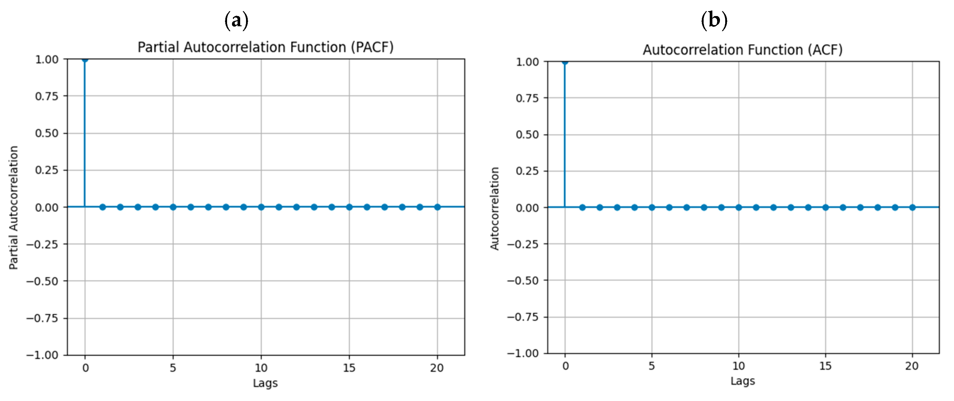
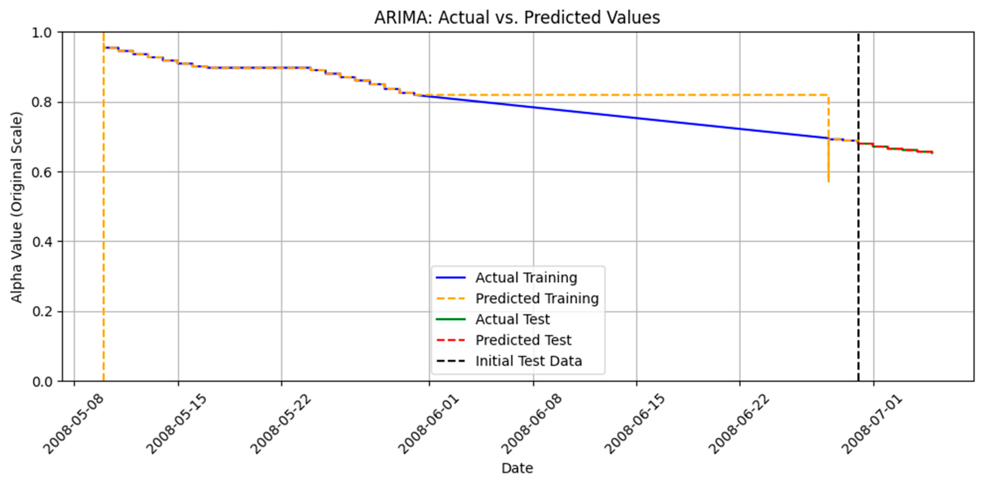
2.7. Methodology for Time Series with ARIMA

To analyze and forecast the time series data of efficiency (α), an Autoregressive Integrated Moving Average (ARIMA) model was employed. The ARIMA(p,d,q) model is a widely used approach for time series forecasting and is characterized by three orders: p, d, and q [47,48,49,50].

The model can be generally expressed using the backshift operator L (where LY_t = Y_t−1) as follows:

$$\left(1-{\sum }_{i=1}^p{ф}_i{L}^i\right){\left(1-L\right)}^d{Y}_t=c+\left(1+{\sum }_{j=1}^q{\theta }_j{L}^j\right){\epsilon }_t$$

(10)

Alternatively, if W_t = ∇^dY_t represents the series after being differenced d times to achieve stationarity, the ARMA(p,q) component for W_t is as follows:

$$W_t=c+{\sum }_{i=1}^p{ф}_i{W}_{t-i}+{\sum }_{j=1}^q{\theta }_j{\epsilon }_{t-j}+{\epsilon }_t$$

(11)

where:

• Y_t is the original time series.
• W_t is the differenced (stationary) series.
• p is the order of the autoregressive (AR) component, indicating the number of lagged observations of the series included in the model.
• d is the order of differencing required to make the series stationary. The first difference is ∇Y_t = Y_t − Y_t−1, and the second difference is∇²Y_t = ∇Y_t –∇Y_t−1.
• q is the order of the moving average (MA) component, indicating the number of lagged forecast errors included in the model.
• ${ф}_i$ are the parameters for the AR terms.
• ${\theta }_j$ are the parameters for the MA terms.
• c is a constant or intercept.
• ${\epsilon }_t$ is the white noise error term at time t, assumed to be independently and identically distributed with a mean of zero and constant variance.

3. Results

Data Analysis

The datasets employed were subjected to preprocessing to elucidate the behavior of the features that exerted the most significant impact. Figure 1 shows a scatter plot with marginal histograms, providing a granular visualization of the relationship between two critical variables: the flow rate (Q) in cubic meters and power (W) in megawatts. The data were stratified into three distinct stages to identify the factors associated with the wear of the hydraulic turbine from which the data were sourced. Each group represents observations collected under varying conditions during May and June.

The graphical representation reveals a distinct linear relationship between the flow rate and generated power across all groups, indicating that an increase in flow rate correlates with an enhancement in power output. Moreover, the slope discerned for each dataset facilitates inferences regarding the impact on the turbine efficiency, particularly because the operational flow rates, as delineated in the flow rate histogram at the top of the graph, are comparable. This aspect, coupled with the data structure in terms of distribution and group variation, provides insights into operational dynamics. The histogram on the right delineates the distributions of the generated power, enabling the observation of variations in the power ranges and the frequency of specific power outputs.

Figure 2a shows a comparison between the actual and predicted values obtained from the linear regression model. The depicted identity line within the graph marks where the predictions perfectly match the actual values. Furthermore, the performance metrics MSE = 5.88 × 10⁻⁵, RMSE = 0.008, MAE = 0.006, and R² = 0.994 indicate that the model provides highly accurate predictions for the majority of the data points. However, there is a noticeable dispersion of points away from the identity line at the extremes of the range, particularly in the lower range [51]. This deviation could be attributed to variable climatic conditions in the area surrounding the hydroelectric plant, as documented in operational reports. Therefore, it is feasible to develop a more robust model that integrates these climatic variables [52]. This enhanced model could potentially identify periods when the turbine was more susceptible to wear and operational variability, provided comprehensive data collection was implemented.

Figure 2b shows a density plot of the residuals derived from the regression analysis. This plot illustrates the deviation between the observed values and those predicted by the model. The distribution configuration, which approximates a skewed bell curve, implies that although a substantial proportion of the residuals clusters near zero, signifying accurate model predictions, a pronounced rightward tail exists. This asymmetry is potentially indicative of the outliers that influence the output of the model. Moreover, the apex of the density curve is situated close to zero, confirming that the majority of the predictions are both precise and exhibit minimal errors. However, the observed skewness might suggest that the capacity of the model to encapsulate the entirety of the data variability is somewhat compromised. This limitation could be attributed to the presence of non-linear relationships within the dataset, which were not adequately addressed by the linear modeling approach. Additionally, extraneous parameters may introduce noise into the model during the training phase, further complicating the accurate representation of the data. At very low or high flow rates, turbine performance deviates from the linear trend due to transient conditions (e.g., startup, shutdown, or rapid demand fluctuations), lower data density, and unmodeled variables like water quality or flow incidence angles. The linear regression model struggles to capture these inherent non-linearities, where efficiency drops sharply, leading to less accurate predictions at the extremes of the performance curve.

Analyzing how each model responds to outliers in the dataset is crucial, particularly when these outliers represent significant events rather than measurement errors. Consequently, a time-series analysis was employed, which facilitated the identification of variations or non-linearities in subsequent analyses, thereby enhancing the model’s generalization capability.

To identify the appropriate order of differencing (d) for the dataset, an initial forecast was attempted with d = 1. However, this resulted in a flat forecast as the model failed to capture the decreasing trend. Subsequently, using d = 2, the model perfectly followed the decreasing linear trend observed in the test set. This indicates that second-order differencing was crucial for the model to identify and project this linear structure.

Following two differentiations (d = 2), an analysis of the Partial Autocorrelation Function (PACF) (Figure 3a) and the Autocorrelation Function (ACF) (Figure 3b) was conducted. The PACF is, by definition, 1 at lag 0. For all subsequent lags (from 1 onwards), the PACF values were practically zero, falling within the confidence band. Similarly, the ACF values for lags greater than 0 were also effectively zero and within the confidence band. This suggests that the appropriate order for the autoregressive (AR) component (p) is 0, and the appropriate order for the moving average (MA) component (q) is also 0. This analysis, where both the PACF and ACF effectively cut off after lag 0, supports an ARIMA (0,2,0) model structure. This implies that after two differencing operations, the resulting series exhibits no significant autocorrelation structure that can be modeled by AR or MA components, resembling white noise.

Figure 4 shows a comparison between the actual and predicted values for both the training and testing datasets within a time-series ARIMA model. Data from July were utilized to assess the temporal series predictions, aiding in visualizing how the model, trained to that date, performs optimally when exposed to new data (test data). The blue and orange lines, representing the actual and predicted values from the training set, respectively, were closely aligned in most instances. This suggests that the model effectively learns the dynamics of the training period. In both datasets, the model captures the general trend of the data. However, there are peaks and troughs that the model does not accurately predict. As previously mentioned, this may be due to uncontrollable aspects of the energy generation process, which is a common challenge in time series where unforeseen events can induce fluctuations that time models fail to capture. The performance metrics for the test data are as follows: MSE Test: 0.0004; R² Test: 0.999.

Overall, it is apparent that there is no need for more robust models, such as neural networks, because, for the phenomena processed, linear relationships adequately generalize the process.

4. Conclusions

This study successfully integrated dimensional analysis (DA) with machine learning (ML) techniques—specifically linear regression and ARIMA time-series modeling—to predict efficiency degradation in Francis turbines operating under sediment-laden flow conditions. The dimensional analysis provided a robust theoretical framework for identifying key operational variables (TIME, Q1, W1) influencing turbine efficiency (α). The ARIMA(0,2,0) model, developed after determining that second-order differencing, was necessary to achieve stationarity and so that no significant autocorrelation remained in the differentiated series, demonstrating exceptional predictive accuracy on the test dataset, achieving an R² value of 0.999 and an MSE of 0.0004. This indicates its strong capability to capture and project the underlying linear trend present in the efficiency data after appropriate differencing.

The findings underscore the importance of appropriate model selection and preprocessing, such as differencing in time-series analysis, to reveal underlying data structures. The high performance of the ARIMA(0,2,0) model suggests that the efficiency degradation, once transformed, follows a predictable linear path, which is invaluable for predictive maintenance scheduling. The dimensional analysis proved beneficial in guiding the initial understanding of relevant variables, although the purely data-driven time-series approach ultimately yielded superior predictive performance for the target variable in this study.

References

1. Ríos, E.H.; Guzmán, J.D.; Ribadeneira, R.; Bailón-García, E.; Acevedo, E.R.; Vélez, F.; Franco, C.A.; Riazi, M.; Cortes, F.B. Effect of the oil content on green hydrogen production from produced water using carbon quantum dots as a disruptive nanolectrolyte. Int. J. Hydrogen Energy 2024, 76, 353–362. [Google Scholar] [CrossRef]
2. Paraschiv, L.S.; Paraschiv, S. Contribution of renewable energy (hydro, wind, solar and biomass) to decarbonization and transformation of the electricity generation sector for sustainable development. Energy Rep. 2023, 9, 535–544. [Google Scholar] [CrossRef]
3. Oyebanji, M.O.; Kirikkaleli, D. Green technology, green electricity, and environmental sustainability in Western European countries. Environ. Sci. Pollut. Res. 2023, 30, 38525–38534. [Google Scholar] [CrossRef]
4. Ohler, A.; Fetters, I. The causal relationship between renewable electricity generation and GDP growth: A study of energy sources. Energy Econ. 2014, 43, 125–139. [Google Scholar] [CrossRef]
5. Sayed, E.T.; Wilberforce, T.; Elsaid, K.; Rabaia, M.K.H.; Abdelkareem, M.A.; Chae, K.-J.; Olabi, A. A critical review on environmental impacts of renewable energy systems and mitigation strategies: Wind, hydro, biomass and geothermal. Sci. Total Environ. 2021, 766, 144505. [Google Scholar] [CrossRef] [PubMed]
6. Fierro, J.J.; Escudero-Atehortua, A.; Nieto-Londoño, C.; Giraldo, M.; Jouhara, H.; Wrobel, L.C. Evaluation of waste heat recovery technologies for the cement industry. Int. J. Thermofluids 2020, 7, 100040. [Google Scholar] [CrossRef]
7. Brough, D.; Jouhara, H. The aluminium industry: A review on state-of-the-art technologies, environmental impacts and possibilities for waste heat recovery. Int. J. Thermofluids 2020, 1, 100007. [Google Scholar] [CrossRef]
8. Mohan, C.; Robinson, J.; Lal, C.; Jammala, A.P.N.; Meena, P.L.; Kumari, N. Sustainable Energy Solutions for Environmental Pollution Control. In Proceedings of the E3S Web of Conferences, Les Mureaux, France, 21–22 November 2024; EDP Sciences: Les Ulis, France; Volume 511, p. 01023. [Google Scholar]
9. Morales, S.; Álvarez, C.; Acevedo, C.; Diaz, C.; Rodriguez, M.; Pacheco, L. An overview of small hydropower plants in Colombia: Status, potential, barriers and perspectives. Renew. Sustain. Energy Rev. 2015, 50, 1650–1657. [Google Scholar] [CrossRef]
10. Barnard, P.L.; Short, A.D.; Harley, M.D.; Splinter, K.D.; Vitousek, S.; Turner, I.L.; Allan, J.; Banno, M.; Bryan, K.R.; Doria, A.; et al. Coastal vulnerability across the Pacific dominated by El Niño/Southern Oscillation. Nat. Geosci. 2015, 8, 801–807. [Google Scholar] [CrossRef]
11. McPhaden, M.J. El Niño and La Niña: Causes and global consequences. Encycl. Glob. Environ. Chang. 2002, 1, 353–370. [Google Scholar]
12. Rosenzweig, C.; Hillel, D. Climate Variability and the Global Harvest: Impacts of El Niño and Other Oscillations on Agro-Ecosystems; Oxford University Press: Oxford, UK, 2008. [Google Scholar]
13. González, O.N.; González, A.N.; Flores, S.M.; Vilchez, F.F. Influence of ENSO and the urban heat island on climate variation in a growing city of the western Mexico. One Ecosyst. 2024, 9, e125302. [Google Scholar] [CrossRef]
14. Thakur, R.; Kumar, A.; Khurana, S.; Sethi, M. Correlation development for erosive wear rate on pelton turbine buckets. Int. J. Mech. Prod. Eng. Res. Dev. 2017, 7, 259–274. [Google Scholar] [CrossRef]
15. Sangal, S.; Singhal, M.K.; Saini, R.P.; Tomar, G.S. Hydro-abrasive erosion modelling in Francis turbine at different silt conditions. Sustain. Energy Technol. Assess. 2022, 53, 102616. [Google Scholar] [CrossRef]
16. Wei, X.-Y.; Pei, J.; Wang, W.-Q.; Yu, Z.-F. Numerical study on sediment erosion characteristics of Francis turbine runner. Eng. Fail. Anal. 2024, 161, 108270. [Google Scholar] [CrossRef]
17. Eltvik, M. Sediment Erosion in Francis Turbines; Institutt for Energi-Og Prosessteknikk: Trondheim, Norwegia, 2009. [Google Scholar]
18. Cruzatty, C.; Jimenez, D.; Valencia, E.; Zambrano, I.; Mora, C.; Luo, X.; Cando, E. A case study: Sediment erosion in francis turbines operated at the san francisco hydropower plant in ecuador. Energies 2021, 15, 8. [Google Scholar] [CrossRef]
19. Thapa, B.S.; Dahlhaug, O.G.; Thapa, B. Sediment erosion in hydro turbines and its effect on the flow around guide vanes of Francis turbine. Renew. Sustain. Energy Rev. 2015, 49, 1100–1113. [Google Scholar] [CrossRef]
20. Khurana, S.; Goel, V. Effect of jet diameter on erosion of turgo impulse turbine runner. J. Mech. Sci. Technol. 2014, 28, 4539–4546. [Google Scholar] [CrossRef]
21. Chitrakar, S.; Neopane, H.P.; Dahlhaug, O.G. Study of the simultaneous effects of secondary flow and sediment erosion in Francis turbines. Renew. Energy 2016, 97, 881–891. [Google Scholar] [CrossRef]
22. Seidel, U.; Mende, C.; Hübner, B.; Weber, W.; Otto, A. Dynamic loads in Francis runners and their impact on fatigue life. IOP Conf. Ser. Earth Environ. Sci. 2014, 22, 032054. [Google Scholar] [CrossRef]
23. Iliev, I.; Trivedi, C.; Dahlhaug, O.G. Variable-speed operation of Francis turbines: A review of the perspectives and challenges. Renew. Sustain. Energy Rev. 2019, 103, 109–121. [Google Scholar] [CrossRef]
24. Tong, D. Cavitation and wear on hydraulic machines. Int. Water Power Dam Constr. 1981, 2, 30–40. [Google Scholar]
25. Masoodi, J.H.; Harmain, G. A methodology for assessment of erosive wear on a Francis turbine runner. Energy 2017, 118, 644–657. [Google Scholar] [CrossRef]
26. Chitrakar, S. FSI Analysis of Francis Turbines Exposed to Sediment Erosion. Ph.D. Thesis, Kathmandu University, Dhulikhel, Nepal, 2013. [Google Scholar]
27. Quaranta, E. Optimal rotational speed of Kaplan and Francis turbines with focus on low-head hydropower applications and dataset collection. J. Hydraul. Eng. 2019, 145, 04019043. [Google Scholar] [CrossRef]
28. Thapa, B.S.; Thapa, B.; Dahlhaug, O.G. Empirical modelling of sediment erosion in Francis turbines. Energy 2012, 41, 386–391. [Google Scholar] [CrossRef]
29. Alrayess, H.; Gharbia, S.; Beden, N.; Keskin, A.U. Using machine learning techniques and deep learning in forecasting the hydroelectric power generation in almus dam, turkey. Safety 2018, 72, 635–647. [Google Scholar]
30. Sapitang, M.; Ridwan, W.M.; Kushiar, K.F.; Ahmed, A.N.; El-Shafie, A. Machine learning application in reservoir water level forecasting for sustainable hydropower generation strategy. Sustainability 2020, 12, 6121. [Google Scholar] [CrossRef]
31. Condemi, C.; Casillas-Pérez, D.; Mastroeni, L.; Jiménez-Fernández, S.; Salcedo-Sanz, S. Hydro-power production capacity prediction based on machine learning regression techniques. Knowl.-Based Syst. 2021, 222, 107012. [Google Scholar] [CrossRef]
32. Di Grande, S.; Berlotti, M.; Cavalieri, S.; Gueli, R. A Machine Learning Approach to Forecasting Hydropower Generation. Energies 2024, 17, 5163. [Google Scholar] [CrossRef]
33. Essenfelder, A.H.; Larosa, F.; Mazzoli, P.; Bagli, S.; Broccoli, D.; Luzzi, V.; Mysiak, J.; Mercogliano, P.; Valle, F.D. Smart climate hydropower tool: A machine-learning seasonal forecasting climate service to support cost–benefit analysis of reservoir management. Atmosphere 2020, 11, 1305. [Google Scholar] [CrossRef]
34. Ekanayake, P.; Wickramasinghe, L.; Jayasinghe, J.M.J.W.; Rathnayake, U.; Hong, T.-P. Regression-Based Prediction of Power Generation at Samanalawewa Hydropower Plant in Sri Lanka Using Machine Learning. Math. Probl. Eng. 2021, 2021, 4913824. [Google Scholar] [CrossRef]
35. Zhang, D.; Wang, D.; Peng, Q.; Lin, J.; Jin, T.; Yang, T.; Sorooshian, S.; Liu, Y. Prediction of the outflow temperature of large-scale hydropower using theory-guided machine learning surrogate models of a high-fidelity hydrodynamics model. J. Hydrol. 2022, 606, 127427. [Google Scholar] [CrossRef]
36. de Souza, J.C.S.; Júnior, O.H.; Filho, G.L.T.; Carpinteiro, O.A.S.; Júnior, H.S.D.B.; dos Santos, I.F.S. Application of machine learning models in predictive maintenance of Francis hydraulic turbines. RBRH 2024, 29, e48. [Google Scholar] [CrossRef]
37. Amini, A.; Pacot, O.; Voide, D.; Hasmatuchi, V.; Roduit, P.; Münch-Alligné, C. Development of a novel cavitation monitoring system for hydro turbines based on machine learning algorithms. IOP Conf. Ser. Earth Environ. Sci. 2022, 1079, 012015. [Google Scholar] [CrossRef]
38. Zhang, J.; Yan, J.; Infield, D.; Liu, Y.; Lien, F.-S. Short-term forecasting and uncertainty analysis of wind turbine power based on long short-term memory network and Gaussian mixture model. Appl. Energy 2019, 241, 229–244. [Google Scholar] [CrossRef]
39. De Castro-Cros, M.; Velasco, M.; Angulo, C. Machine-learning-based condition assessment of gas turbines—A review. Energies 2021, 14, 8468. [Google Scholar] [CrossRef]
40. Duan, R.; Liu, J.; Zhou, J.; Liu, Y.; Wang, P.; Niu, X. Study on performance evaluation and prediction of francis turbine units considering low-quality data and variable operating conditions. Appl. Sci. 2022, 12, 4866. [Google Scholar] [CrossRef]
41. Srivastava, T.; Vedanshu; Tripathi, M.M. Predictive analysis of RNN, GBM and LSTM network for short-term wind power forecasting. J. Stat. Manag. Syst. 2020, 23, 33–47. [Google Scholar] [CrossRef]
42. Wang, Y.; Xie, D.; Wang, X.; Zhang, Y. Prediction of wind turbine-grid interaction based on a principal component analysis-long short term memory model. Energies 2018, 11, 3221. [Google Scholar] [CrossRef]
43. Xiao, X.; Liu, J.; Liu, D.; Tang, Y.; Zhang, F. Condition monitoring of wind turbine main bearing based on multivariate time series forecasting. Energies 2022, 15, 1951. [Google Scholar] [CrossRef]
44. Xiong, L.; Liu, J.; Song, B.; Dang, J.; Yang, F.; Lin, H. Deep learning compound trend prediction model for hydraulic turbine time series. Int. J. Low-Carbon Technol. 2021, 16, 725–731. [Google Scholar] [CrossRef]
45. Truscott, G. A literature survey on abrasive wear in hydraulic machinery. Wear 1972, 20, 29–50. [Google Scholar] [CrossRef]
46. Nozaki, T.; Takayanagi, T. Estimation of repair cycle of turbine due to abrasion caused by suspended sand and determination of capacity and cross section of desilting basin. Dengen Kaihatsu KK Chosa Shiryo 1987, 81, 68–98. [Google Scholar]
47. Chen, J.-F.; Wang, W.-M.; Huang, C.-M. Analysis of an adaptive time-series autoregressive moving-average (ARMA) model for short-term load forecasting. Electr. Power Syst. Res. 1995, 34, 187–196. [Google Scholar] [CrossRef]
48. Rojas, I.; Valenzuela, O.; Rojas, F.; Guillen, A.; Herrera, L.; Pomares, H.; Marquez, L.; Pasadas, M. Soft-computing techniques and ARMA model for time series prediction. Neurocomputing 2008, 71, 519–537. [Google Scholar] [CrossRef]
49. Shumway, R.H.; Stoffer, D.S.; Shumway, R.H.; Stoffer, D.S. ARIMA models. In Time Series Analysis and Its Applications: With R Examples; Springer: Berlin/Heidelberg, Germany, 2017; pp. 75–163. [Google Scholar]
50. Valipour, M.; Banihabib, M.E.; Behbahani, S.M.R. Comparison of the ARMA, ARIMA, and the autoregressive artificial neural network models in forecasting the monthly inflow of Dez dam reservoir. J. Hydrol. 2013, 476, 433–441. [Google Scholar] [CrossRef]
51. Friede, M.; Ehlert, S.; Grimme, S.; Mewes, J.-M. Do Optimally tuned range-separated hybrid functionals require a reparametrization of the dispersion correction? It Depends. J. Chem. Theory Comput. 2023, 19, 8097–8107. [Google Scholar] [CrossRef]
52. Cheng, Q.; Liu, P.; Xia, J.; Ming, B.; Cheng, L.; Chen, J.; Xie, K.; Liu, Z.; Li, X. Contribution of complementary operation in adapting to climate change impacts on a large-scale wind–solar–hydro system: A case study in the Yalong River Basin, China. Appl. Energy 2022, 325, 119809. [Google Scholar] [CrossRef]
Figure 1. Scatter plot with marginal histograms for the flow rate (Q) in cubic meters and the power in MW (W).
Energies 18 04023 g001
Figure 2. (a) Comparison between actual and predicted values, and (b) density plot of residuals.
Energies 18 04023 g002
Figure 3. (a) Partial Autocorrelation Function (PACF), p = 0. (b) Autocorrelation Function (ACF), q = 0 for the differenced series.
Energies 18 04023 g003
Figure 4. Comparison between actual and predicted values for both training and test dataset in a time-series model.
Energies 18 04023 g004