Abstract
With the increasing integration of renewable energy and smart technologies in residential energy systems, proactive household energy management (HEM) have become critical for reducing costs, enhancing grid stability, and achieving sustainability goals. This study proposes a ultra-short-term forecasting-driven proactive energy consumption optimization strategy that integrates advanced forecasting models with multi-objective scheduling algorithms. By leveraging deep learning techniques like Graph Attention Network (GAT) architectures, the system predicts ultra-short-term household load profiles with high accuracy, addressing the volatility of residential energy use. Then, based on the predicted data, a comprehensive consideration of electricity costs, user comfort, carbon emission pricing, and grid load balance indicators is undertaken. This study proposes an enhanced mixed-integer optimization algorithm to collaboratively optimize multiple objective functions, thereby refining appliance scheduling, energy storage utilization, and grid interaction. Case studies demonstrate that integrating photovoltaic (PV) power generation forecasting and load forecasting models into a home energy management system, and adjusting the original power usage schedule based on predicted PV output and water heater demand, can effectively reduce electricity costs and carbon emissions without compromising user engagement in optimization. This approach helps promote energy-saving and low-carbon electricity consumption habits among users.
1. Introduction
As an essential component of demand-side resource management, Home Energy Management Systems (HEMs) aim to achieve optimized household electricity scheduling through advanced technologies. They enhance energy efficiency, reduce users’ electricity costs, and promote the effective utilization of renewable energy sources [1]. Driven by the digital transformation of the power grid, residential electricity consumption patterns are gradually evolving toward intelligent control, personalized customization, and flexible interaction. This shift requires HEMs to further enhance their demand response capabilities, coordinating household electricity usage with grid operations more efficiently [2].
Load forecasting technologies can predict the total electricity consumption or household PV generation over a future period [3,4]. By mining the demand response potential based on load forecasting results, it becomes possible to proactively plan demand response resources, laying a critical foundation for achieving supply-demand balance. Power supply companies can formulate personalized time-of-use pricing and demand response incentive policies based on the forecasting results and the specific electricity consumption characteristics of different households [5]. Meanwhile, residential users can develop PV generation, energy storage, and electricity usage strategies in advance, based on forecasting outcomes, to maximize their demand response participation without affecting daily life, thus enabling friendly supply-demand interaction.
As the share of renewable energy sources such as PV and wind power increases in the power grid, their inherent volatility introduces greater uncertainty and complexity. This, in turn, places higher demands on the accuracy and granularity of demand-side load forecasting. Ultra-short-term load forecasting with hourly-level granularity has become a key technology for supporting flexible regulation in new power systems. Compared with day-ahead forecasting, intra-day, hourly-level ultra-short-term forecasting can more accurately capture sudden fluctuations such as PV output drops and random electric vehicle charging events. It provides a critical time window for electricity optimization and dispatching and effectively addresses the power oscillations caused by the coupling of supply and demand randomness under high renewable penetration. This lays the foundation for constructing a new HEMs paradigm that enables both proactive planning and rapid response [6].
Machine learning and deep learning-based models are increasingly applied in load forecasting. Deep learning technologies, by constructing multi-layer neural network architectures such as Back Propagation Neural Networks (BPNN) [7], Long Short-Term Memory Networks (LSTM) [8], and Temporal Convolutional Networks (TCN) [9], effectively capture nonlinear features in time-series data. However, single-model-based approaches still fall short in deeply extracting temporal features, limiting their prediction accuracy. Reference [10] utilized LSTM neural networks to forecast total power consumption. However, LSTM models only capture long-term dependencies in time series and cannot explicitly model the relationships between electricity consumption data and environmental variables like temperature and humidity. They also require manual integration of multi-source data and cannot dynamically adjust the importance of different data sources. Reference [11] adopted Convolutional Neural Networks (CNNs) to extract internal features from the generator in Conditional Generative Adversarial Networks (CGANs), generating synthetic samples to reduce prediction error and enhance model representation capabilities. However, CNN kernels are only capable of capturing local spatial features and struggle to model long-range dependencies among distant devices. Reference [12] applied CNNs to extract information from time-series data with uncertain features and employed Gated Recurrent Units (GRUs) for time-series forecasting, achieving improved prediction accuracy compared to CNNs alone. In this study, the Graph Attention Network (GAT) is employed to achieve intra-day rolling forecasting of household energy consumption by capturing deep correlations between historical user behavior data and external dynamic environmental factors (e.g., temperature and humidity). Unlike conventional sequence models such as LSTM and GRU, GAT enables higher-dimensional integration of cross-appliance interactions and environmental dependencies, thereby enhancing predictive accuracy through attention-based learning of spatiotemporal patterns. With the increasing prevalence of distributed photovoltaic (PV) installations and the continuous rise in residential electricity consumption, household energy usage is undergoing a profound shift from simple electricity consumption to a “source-storage-load interaction” model. This significant transformation in energy consumption structure has elevated HEMs from being mere electricity management tools to intelligent hubs that bridge the supply and demand sides, balancing individual diversified energy needs with system-level operational objectives. Farrokhifar et al. [13] developed a household energy model incorporating flexible appliance usage models and operational constraints. They formulated an optimization scheduling plan aimed at minimizing electricity costs under a time-of-use pricing mechanism using integer linear programming, significantly reducing electricity bills compared to the unoptimized scenario. Oureshi et al. [14] integrated smart communication technologies with real-time monitoring devices, designing a HEMs control architecture that uses sensor networks for monitoring and aims to reduce peak electricity demand. This system can automatically optimize appliance operating times and generate intuitive billing information to help users save on electricity costs. Jaradat et al. [15] introduced a visual interface that converts energy consumption data from flexible appliances like air conditioners and water heaters into graphs or alerts, guiding users to actively adjust their electricity usage habits. However, the above studies only considered household appliances and ignored the impacts of distributed generation, energy storage systems, and electric vehicles. In response to the growing adoption of household PV and storage devices, Reference [16] designed a dynamic scheduling strategy to coordinate the operation of various device types, focusing on ensuring power supply stability and reducing overall household electricity expenses under distributed renewable energy and storage systems. Reference [17] addressed PV generation, battery charging/discharging, and thermal load scheduling in HEMs construction. Based on established PV and thermostatically controlled load models, they proposed an optimal operation strategy for microgrids to minimize total operating costs. Reference [18] used sensor networks to collect microgrid operational data and appliance usage information, applying machine learning methods to plan energy resources. However, this type of HEMs, which relies on intrusive data acquisition devices, incurs high installation and maintenance costs.
With the growing intelligence of electric vehicles (EVs) and advancements in communication technologies, EVs now possess the remote connectivity needed to interact flexibly with the grid, serving as a powerful supplement to end-user energy storage. Yang et al. [19] utilized the storage capacity of plug-in hybrid electric vehicles (PHEVs) to absorb excess solar PV energy and supply power to homes during outages. Yousefi et al. [20] integrated PHEVs, PV arrays, and heat pumps into a system that updates optimization strategies in real time based on load forecasts, ensuring that electricity usage plans meet household load demands, PEV battery charging requirements, and thermal comfort conditions. Reference [21] explored a renewable energy-driven residential energy hub integrating combined heat and power (CHP), PHEVs, thermal storage units, PV systems, and conventional appliances. They developed an optimization model aimed at minimizing energy costs, enabling coordinated operation of multiple components at optimal cost. However, while these studies achieved coordinated optimization of appliances, PV, storage, and EVs, most were limited to system architecture design and lacked exploration into behavioral drivers that influence user participation, such as sensitivity to electricity costs, comfort preferences, and response incentives.
For most users, minimizing electricity costs remains the primary objective. HEMs receive time-of-use pricing, real-time pricing, and peak pricing information in real time, executing optimized scheduling algorithms based on household consumption habits and appliance characteristics. Reference [22] aimed to minimize peak-period electricity demand and utility bills using a particle swarm optimization algorithm to shift loads from peak to off-peak periods, significantly reducing both peak-period energy use and utility costs. Sarker et al. [23], to reduce peak demand, peak-to-average ratio, and energy costs, proposed shifting household loads based on time-of-use pricing. By integrating PV generation with demand response management, they reduced electricity purchases and sold excess PV energy to the grid, significantly lowering total household electricity costs. Huang et al. [24] introduced energy storage into HEMs to address supply-demand mismatches in homes. Combined with real-time grid pricing, they developed a model to minimize electricity purchase costs and enhance renewable energy utilization, achieving arbitrage between low storage and high feed-in prices and enabling spatial-temporal shifting of household energy demand. Reference [25] proposed a novel co-operative household microgrid energy scheduling control strategy. Based on time-of-use pricing, it allows bi-directional electricity trading between households and the grid, as well as renewable energy trading among households, thereby reducing the grid’s overall energy supply demand.
In addition to optimizing appliance operation and reducing electricity purchased from the grid, actively participating in demand response programs to receive incentive payments is also an effective way for users to cut costs. Demand response incentives refer to payments or subsidies issued by aggregators based on users’ actual load reductions, encouraging participation in demand-side management programs. Reference [26] combined reinforcement learning with demand response incentive mechanisms to propose an optimization model that learns user behavior in real-time and dynamically adjusts incentive strategies, thereby optimizing household energy scheduling and reducing electricity expenses. Reference [27] evaluated the effects of different incentive strategies under microgrid operational constraints, showing that suitable pricing mechanisms and incentives can effectively shift household energy consumption patterns, optimize overall grid load, and improve energy efficiency. To further stimulate user participation in demand response, Reference [28] compared a HEMs model based on time-of-use pricing with one incorporating both time-of-use pricing and demand response incentives. Results showed that the latter increased user benefits by more than 14%. However, existing HEMs studies mostly focus on the electricity perspective and overlook carbon reduction potential on the user side. In the context of grid decarbonization, carbon trading is gradually extending to residential users. Integrating carbon trading mechanisms into HEMs frameworks can promote local consumption of distributed renewable energy and effectively reduce overall system carbon emissions. Based on this, reference [29] proposed a HEMs model for low-carbon operation from an “electricity-carbon coupling” perspective, introducing a weighting factor to represent the consumption preferences of different customer types. However, this study used a fixed carbon price model, which does not reflect the relationship between emissions and price. Tiered carbon pricing, which dynamically adjusts prices based on emission levels, has been shown to provide better incentives for emission reduction [30]. Reference [31] developed a two-layer optimization model considering both peak load reduction commands and daily operating costs. By comparing traditional scheduling with comprehensive demand response models, they demonstrated the advantages of tiered carbon trading mechanisms in reducing emissions and energy costs. Reference [32] innovatively incorporated tiered carbon trading into capacity configuration of wind-solar-hydrogen-storage systems, establishing a life-cycle cost optimization model and solving it with combined AC/DC control strategies and intelligent algorithms, significantly enhancing the low-carbon performance of microgrids. However, this study only considered the carbon trading mechanism and did not address the challenges of grid stability posed by introducing tiered carbon trading under source-load uncertainty.
Most of the existing research focuses on optimizing household economics, while neglecting subjective comfort considerations. Residential electricity activities are characterized by spontaneity and subjectivity, and ignoring comfort needs may lead to user resistance to scheduling strategies. To address this, Reference [33] quantified user discomfort as a linear function of the time shift of appliance usage and developed a scheduling model balancing electricity cost and comfort. Reference [34] assessed user acceptance of flexible appliance schedules (e.g., washing machines and dishwashers) using a time-shift tolerance model and introduced the concept of “random rejection” probability due to external environmental disturbances. Reference [35] propose a new smart system approach for the characterization of the appliance load signature based on a data-driven method, namely the phase diagram, to use the non-intrusive load monitoring of appliances in order to recognize different types of consumers that can exist within a smart building. Reference [36] proposes a phase diagram-based NILM approach that uses voltage-current trajectories to identify individual appliances. The method demonstrates effective load disaggregation with minimal computational overhead. Reference [37] introduces a robust NILM method based on phase space reconstruction (PSR) and ensemble classifiers. By reconstructing high-dimensional state trajectories from current-voltage data, the method captures non-linear appliance behavior and achieves high classification accuracy under noisy and dynamic conditions. However, these studies focused only on time-preference comfort and did not explore thermal comfort. Thermostatically controlled devices such as air conditioners and water heaters are highly flexible and account for a significant share of energy consumption. Studying their scheduling potential can better support fine-grained load management and the low-carbon transition of power systems.
In summary, existing research on home energy management presents the following limitations:
- Insufficient methods for addressing the volatility of PV and the randomness of household loads; there is a lack of proactive household energy optimization strategies.
- Most studies focus on balancing a limited number of energy objectives. However, with the trends toward diversified household energy demands and low-carbon development, further research is needed to achieve coordinated optimization of load balancing, cost control, carbon emissions, user comfort, and demand-side response. It is crucial to meet both household economic and comfort needs while ensuring the grid’s low-carbon, efficient, and stable operation.
To address the above challenges, this paper proposes a proactive household energy optimization strategy based on ultra-short-term forecasting. First, an intra-day, hourly-level rolling forecasting mechanism is established for PV output and household electricity consumption, addressing scheduling uncertainty and response delays caused by PV intermittency and load randomness. Then, a multi-factor collaborative optimization objective function is proposed, incorporating electricity cost, user comfort, carbon pricing, and grid load balancing indicators. An improved mixed-integer optimization method is used to solve the problem.
The main contribution of this paper is as follow:
- (1)
- A dual stream ultra-short term forecasting framework based on GAT;
- (2)
- A hybrid GA B&B solution strategy for mixed integer scheduling;
- (3)
- A four objective normalized optimization model;
- (4)
- Extensive multi scenario simulations demonstrating effectiveness.
The remainder of this paper is organized as follows. Section 2 presents the overall architecture of the proposed proactive home energy management system, detailing the roles of key components such as PV panels, smart meters, non-intrusive load monitoring (NILM), and the forecasting module. Section 3 describes the modeling and optimization framework, including the ultra-short-term forecasting module based on a dual-stream Graph Attention Network (GAT), the formulation of the four normalized optimization objectives, and the hybrid GA–Branch-and-Bound algorithm used for mixed-integer scheduling. Section 4 reports on simulation results and experimental validation, comparing different management scenarios and evaluating the performance of the forecasting and optimization modules. Section 5 concludes the paper and discusses the limitations of the proposed method, as well as possible directions for future research.
2. HEMs
2.1. HEMs Architecture Based on Ultra-Short-Term Forecasting
Current HEMs face multiple technical challenges. First, PV output is significantly affected by weather conditions, and the error in intra-day ultra-short-term power forecasting directly impacts the robustness of energy storage scheduling. Second, under mechanisms such as time-of-use electricity pricing, demand response, and carbon trading, users must perform multi-objective trade-offs among electricity price signals, carbon emission costs, and energy usage comfort. Traditional HEMSs increasingly show limitations in addressing both source-load uncertainties, protecting user privacy, and supporting diversified demand responses. Therefore, there is an urgent need for functional upgrades through technological innovations.
The rapid development of smart meters, artificial intelligence, and the Internet of Things provides new solutions to overcome these bottlenecks. The proposed HEMS architecture based on ultra-short-term forecasting is illustrated in Figure 1. As shown in the figure, the HEMs architecture integrates smart meters, PV generation systems, weather forecast service interfaces, and household environmental data sensors to collect real-time multi-source data, including household electricity usage, PV output, high-resolution weather forecasts, and indoor/outdoor temperature and humidity. These data are stored on the HEMS server.
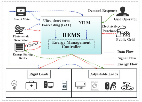
Figure 1.
The HEMS architecture based on NILM and ultra-short-term prediction.
The built-in non-intrusive load monitoring (NILM) unit is capable of real-time recognition of the operational status of various appliances. Based on the recognition results, the system analyzes and mines user behavior patterns (detailed implementation can be found in our previous work [38]). Simultaneously, HEMs can access pre-trained deep learning model parameters and continuously run forecasting models using local computing resources. By combining real-time meteorological, environmental, and historical consumption data, it dynamically predicts the PV output and electricity demand for the upcoming hour. Finally, the user behavior analysis and prediction results are input into the energy management controller, which employs a multi-factor system optimization algorithm to generate more accurate energy usage strategies.
2.2. System Model
2.2.1. Appliance Load Model
The HEMs proposed in this study primarily considers three types of electrical loads: rigid loads, adjustable loads, and energy storage devices, and performs energy management accordingly. Suppose the load optimization and scheduling horizon is divided into T time intervals, each with a duration of , the models for each type of load are described as follows:
- (1)
- Household Load Model
In residential energy management systems, non-deferrable or inflexible loads denote appliances that require continuous operation and cannot be easily shifted or turned off, such as lights, refrigerators, and essential medical devices. These types of loads exhibit minimal flexibility in terms of scheduling and are typically recognized as the fundamental power consumption of a household—commonly referred to as the baseline demand. The usage periods of such fixed-function devices are largely predetermined, as they support essential daily functions including illumination, cooling, and maintaining internet connectivity via routers.
For rigid loads with relatively stable power demand and fixed operation time, their power consumption can be expressed as shown in Equation (1).
where denotes the power of the rigid load n at time t, and is the rated power of the load.
- (2)
- Adjustable Loads
Adjustable loads refer to those electrical devices whose operation will be adjusted or modified within a certain range in response to grid requirements or economic incentives. Different from rigid loads, the operating time and power of adjustable loads can be flexibly modified based on scheduling strategies. For example, adjustable loads can shift their operating periods or reduce their power consumption to improve overall energy efficiency and reduce electricity costs. According to their scheduling properties, adjustable appliances can be divided into three types: those with flexible power levels, those with flexible operating times, and those that allow adjustments in both power and time dimensions.
- (a)
- Power-Adjustable Loads
Power-adjustable loads are devices whose output power can be controlled by switching among multiple power levels. Common examples include air conditioners and water heaters. During their operation, the energy consumption can be effectively regulated by adjusting the power level settings. These types of loads can be modeled using discrete power levels. Assuming each device has several power levels (e.g., low, medium, and high), the output power at time interval ttt is determined by the selected power level, as shown in Equation (2):
where is the power of the adjustable load n at time interval t, and is the power value corresponding to the i-th power level.
- (b)
- Time-Adjustable Loads
Time-adjustable loads refer to energy-consuming devices whose start time can be flexibly scheduled according to operational requirements, such as washing machines and dishwashers. The key characteristic of these loads is that their start time can be shifted, but once the operation begins, they must run continuously for a specified duration at a fixed power level. During operation, the output power is not adjustable. Assuming a time-adjustable load is allowed to start no earlier than time and must complete its operation no later than , the model is described by Equations (3) and (4):
where is the power of the time-adjustable load n at time interval t, and is the operation duration of the load.
The scheduling constraint for time-adjustable loads is expressed as Equation (5):
which means the device must start operation no later than , and once started, the operation cannot be interrupted.
- (c)
- Power-Time Adjustable Loads
Power-time adjustable loads refer to a category of highly flexible demand-side resources that exhibit both temporal scheduling flexibility and the ability to be interrupted during operation. Representative examples include electric vehicles (EVs) and emerging clean transportation systems. Owing to their significant controllability, these loads are often given priority in demand response programs. In practical applications, they are sometimes viewed as analogous to energy storage units, albeit without an actual discharging phase.
Such loads can be characterized by a function where both the power level and operational timing are modifiable within a specified scheduling window. For example, the charging cycle of an EV can be deferred or paused at any point within its allotted charging period, thus making it a highly manageable and adaptive form of load.
The constraints for EV charging/discharging power and battery energy level are defined as follows:
where is the energy state of the EV battery at time t. and are the lower and upper bounds of usable battery capacity. and are the charging/discharging efficiencies. and are the charging/discharging power at time t. and are the maximum charging/discharging power limits. and are the EV grid connection and departure times.
The EV’s energy level at time t is determined recursively, as shown in Equation (10):
EVs, as controllable loads, exhibit uncertainty in connection time, disconnection time, and state of charge. However, behavioral characteristics like typical charging time, duration, and energy consumption per trip show regular patterns. By mining users’ recent travel data, the probability distribution of EV connection status can be estimated. A probabilistic model can then be built to simulate its load demands and constrain behavior such as grid-in time, grid-out time, and charging duration. To meet the user’s daily travel requirements, the EV must satisfy the energy level constraint at departure, as given in Equation (11):
where is the energy level at the departure time, and is the desired energy level for travel.
- (3)
- Energy Storage Devices
In residential energy storage systems, batteries are typically used to store surplus PV energy for later use. The energy storage device model mainly focuses on changes in battery state during charging and discharging processes. To prolong battery life, charging and discharging operations are only allowed when the battery’s energy level reaches certain thresholds. The battery energy dynamics during charging and discharging are governed by Equation (12):
where is the battery energy state at time t. and are the charging and discharging efficiencies, respectively. and are the charging and discharging power at time t.
To extend the service life of the battery and slow down degradation, the system ensures that charging and discharging do not occur simultaneously. Additionally, constraints are imposed on the maximum charging/discharging power and the energy capacity of the battery, as given by the following equations:
where and are the upper and lower limits of usable battery energy. and are the maximum charging and discharging powers, respectively.
2.2.2. Time-of-Use Pricing and Demand Response Model
- (1)
- Time-of-Use (TOU) Pricing Mechanism
The TOU pricing mechanism is a rate system based on electricity market price variations that encourages users to consume electricity during off-peak periods and reduce usage during peak periods. According to the load patterns at different times of the day, electricity prices are categorized into three types: peak, flat, and off-peak rates. For example, during peak hours (such as weekday mornings and evenings), electricity prices are higher due to greater demand; conversely, prices are lower during off-peak periods (such as late at night). Additionally, during extreme peak demand events, prices may be temporarily increased to incentivize users to reduce consumption and help alleviate grid stress. The TOU pricing model is represented by Equation (16):
- (2)
- Demand Response Compensation
Demand response (DR) is a load management strategy used in power systems to encourage users to adjust their energy usage during periods of high grid load or high electricity prices, thereby improving system stability and economic efficiency. To incentivize participation in DR programs, grid operators or utility companies often provide financial compensation to users who reduce electricity consumption during peak demand events.
DR compensation mainly includes rewards for load reduction and incentives for load shifting. The compensation amount is calculated based on the reduction in user load during DR events, encouraging electricity usage during off-peak periods with corresponding subsidies. In home energy management systems, a dynamic incentive mechanism is adopted, where real-time electricity prices are used to adjust the level of subsidy. For the t-th time slot, the incentive subsidy is calculated as shown in Equation (17):
where represents the base incentive, in yuan/kWh. denotes the adjusted user load in the t-th time slot, in kWh. The total incentive subsidy is the sum of the subsidies over all time periods, which not only enables dynamic load regulation but also helps balance grid operations and reduce electricity costs.
2.2.3. Carbon Emissions
Carbon emissions typically denote the aggregate output of carbon dioxide and other greenhouse gases resulting from energy-related activities. In residential settings, primary emission sources encompass electricity consumption, space heating, and gas-fueled cooking, which contribute to both direct and indirect emissions. In contrast, carbon consumption reflects the portion of a household’s carbon allowance that is depleted through its energy use, effectively translating energy expenditure into a carbon-based metric. Variations in carbon pricing can significantly impact user behavior, potentially motivating households to modify their electricity consumption patterns.
To reflect this, a tiered carbon trading mechanism is introduced. This mechanism divides carbon emission responsibility into several brackets—higher levels of emissions correspond to higher unit carbon trading prices.
Assuming the power exchanged between the household microgrid and the main grid is , then the carbon emissions during time period t and the net grid exchange power can be calculated as shown in Equations (18) and (19):
where is carbon emission intensity of the local grid (kg CO2/kWh) which updated hourly based on grid carbon intensity data. , , is the number of rigid, adjustable-power, and time-shiftable loads, respectively. and is the power exchanged by the electric vehicle and battery energy storage with the grid at time t. and is binary indicators (0 or 1) denoting whether the EV or battery is interacting with the grid. is the power output from photovoltaic generation at time t. As indicated in Equation (19), household carbon emissions are closely linked to the source of electricity. Maximizing local consumption of PV energy is an effective strategy to reduce carbon emissions.
3. Methodology
3.1. Optimization Objective
- (1)
- Electricity Cost
Household electricity cost includes the expenses of purchasing electricity from the grid, demand response incentives, as well as the operational and maintenance (O&M) costs of electric vehicles (EVs) and energy storage systems (ESS). The electricity cost objective function is shown in Equation (20).
where represents the electricity purchase cost from the grid during time period t. and , respectively represent the battery degradation cost of the electric vehicle and the energy storage system, which are calculated as follows:
where DEV and DSOC represent the unit energy operation and maintenance cost coefficients for the electric vehicle and the energy storage system, respectively, and the values are set based on the reference [24].
- (2)
- User Comfort
In optimizing residential electricity consumption, it is crucial to find a balance between minimizing energy costs and preserving user comfort. Neglecting user satisfaction may reduce engagement in demand-side management initiatives. Within home energy systems, user comfort refers to the extent to which individuals are willing to accept scheduling changes or demand response measures without experiencing a decline in quality of life or convenience. This subjective factor is shaped by variables such as indoor temperature preferences, appliance usage routines, tolerance for delays, and overall lifestyle. Accurate representation of comfort levels in models can support energy-efficient operation while ensuring the user’s experience remains satisfactory.
User comfort is commonly broken down into two components: temporal comfort and thermal comfort. Temporal comfort reflects how well the timing of appliance operation aligns with the user’s intended or preferred usage schedule. For instance, if a user expects the washing machine to run between 8:00 p.m. and 10:00 p.m., but it starts at 7:00 p.m. or 11:00 p.m. instead, dissatisfaction may occur. Similarly, scheduling the charging of an electric vehicle outside of the desired window—for example, charging between 6:00 a.m. and 8:00 a.m. when the vehicle is needed by 6:00 a.m.—can disrupt daily routines.
In this study, temporal comfort is measured through a piecewise time-based coefficient, which quantifies the degree of alignment between the scheduled operation of appliances and users’ habitual usage windows. It is defined as:
where is the time comfort level of device n at time t. is the probability density that device n operates during time t. is a binary variable indicating whether device n is on (1) or off (0) at time t. is the probability threshold for defining the most comfortable operating interval. is the threshold for the acceptable adjustable interval.
Temperature comfort refers to the user’s satisfaction with indoor temperature, typically regulated by HVAC systems such as air conditioning, heating, or underfloor heating. Influencing factors include the user’s target temperature and acceptable temperature fluctuation range. Let the user’s comfort temperature range be . When the indoor temperature is within this range, users feel comfortable. If the temperature deviates, comfort decreases. The degree of deviation is shown in Equation (25):
where is the deviation of indoor temperature from the comfort temperature. In our model, thresholds such as Temin and Temax are set based on standardized thermal comfort bands (e.g., 22–26 °C for summer cooling) recommended by reference [13].
To link AC power consumption to indoor temperature changes, we adopt a simplified thermal response model that captures the first-order dynamics of a single-zone building. The indoor temperature at time t + 1 is computed as: Teroom(t + 1) = Teroom(t) + α·(Teout(t) − Teroom(t)) − β·PAC(t), where Teout(t) is the outdoor temperature, PAC(t) is the AC cooling power input (kW), α is the thermal conductance coefficient (e.g., 0.1/°C), and β is the cooling efficiency (e.g., 0.5 °C/kWh). This equation reflects the competing effects of passive heat gain/loss and active cooling. These parameters can be calibrated based on empirical data or set according to typical residential envelope characteristics. This model enables dynamic estimation of Teroom, ensuring temperature comfort constraints are physically respected.
The human body perceives temperature changes non-linearly—discomfort increases as deviation grows. Based on this, the temperature comfort function is calculated using Equation (26):
Finally, the overall user electricity comfort level fU is the sum of time comfort and temperature comfort, as shown in Equation (27):
where both temperature and time-preference utilities are normalized to [0, 1].
- (3)
- Carbon Emission Cost
A tiered carbon trading mechanism is introduced, which divides carbon emission responsibilities into multiple intervals. The higher the carbon emissions, the higher the unit price for carbon trading. The expression for the tiered carbon emission cost is shown in Equation (28):
where is the base carbon trading price in time period t. is the length of the carbon emission penalty interval. is the penalty coefficient for carbon trading price. These parameters are calibrated based on national carbon pricing scenarios and DR (Demand Response) program. λ is set at 0.2–0.5 based on sensitivity ranges in reference [13], and d is aligned with TOU billing periods (e.g., 1-h intervals).
- (4)
- Load Balancing
In the context of residential energy management, load balancing aims to maintain a relatively stable electricity demand profile over time, minimizing extreme variations or peak load occurrences. A well-leveled load curve contributes not only to reducing household electricity expenses but also to easing stress on the electrical grid, improving overall energy utilization, and promoting the seamless incorporation of renewable energy sources.
The degree of load balance is often assessed based on the smoothness of the net load curve—defined as the household’s total electricity usage minus the output generated from local renewable systems such as photovoltaic panels. Several quantitative metrics can be used to evaluate load curve smoothness, including peak-to-valley load differences, statistical measures like standard deviation, and the maximum fluctuation between consecutive time slots. In this research, we adopt a comprehensive evaluation strategy that accounts for the average and variability of system load, the full range of load amplitude, and the correlation between control parameters and load variation, to quantify the flatness of the net load curve. The specific calculation process is as follows:
- (1)
- Let P(t) denote the system load at time t.
- (2)
- The mean system load over a period T is calculated as Equation (29):
- (3)
- The degree of load fluctuation (standard deviation) is calculated as Equation (30):
- (4)
- From the load fluctuation, the baseline flatness of the system is derived as Equation (31):
- (5)
- Let Psoft(t) denote the total power of flexible loads at time t, and let be its mean. The matching degree between control variables and load fluctuations is expressed in Equation (32):
- (6)
- The final load flatness indicator is defined in Equation (33):where fH is processed by min–max normalization to ensure its value lies in [0, 1].
3.2. Optimization Objective
To address the problem of household load optimization scheduling, this study comprehensively considers electricity cost, user comfort, carbon emission cost, and the load balancing indicator, aiming to develop a rational electricity usage optimization strategy. The model is based on inputs such as PV generation, electricity price, ambient temperature, rigid loads, and controllable (flexible) loads, and it optimizes the operation periods of various appliances to minimize electricity cost. The objective function is defined as shown in Equation (34):
where , , and are the weights corresponding to the sub-objectives fE, fCE, fU and fH, respectively. Considering that these four sub-objectives have different units and scales, normalization is applied to balance their influence on the scheduling results in terms of economy, comfort, and load smoothness. The normalization method is shown in Equation (35):
where is the normalized value of a given sub-objective, and represent the maximum and minimum values of this objective across all scheduling periods.
3.3. Hybrid Genetic and Branch-and-Bound Algorithm
To solve the objective function for electricity optimization, this study proposes a hybrid Genetic and Branch-and-Bound (GA-B&B) algorithm. This algorithm integrates the precision of the Branch-and-Bound method with the efficiency of the Genetic Algorithm, effectively addressing the limitations of conventional B&B, such as high computational complexity and slow upper-lower bound convergence. The proposed hybrid approach enables efficient solving of the electricity optimization objective function.
The objective function is formulated as a Mixed-Integer Linear Programming (MILP) problem, involving four sub-objectives: electricity cost, user comfort, carbon emission cost, and load balancing indicator. The GA-B&B algorithm accelerates convergence by dynamically generating high-quality feasible solutions, thereby improving the solving efficiency.
The solution process is divided into five steps, as follows:
- Step 1:
- Initialization
First, the integer variables in the MILP are encoded into genetic sequences. An initial population of 50 individuals is randomly generated. The fitness of each individual is evaluated, and the best solution is recorded. The objective value of the best solution is set as the global upper bound (UB), and the lower bound (LB) is initialized to negative infinity. The original MILP problem is then added as the root node to the active node queue, which is sorted by the LP relaxation value, preparing for the subsequent Branch-and-Bound process.
- Step 2:
- Relaxation and Pruning
For the current node, Linear Programming (LP) relaxation is performed to obtain the relaxed solution and its objective value .
- If no feasible solution exists, the branch is pruned directly.
- If a feasible solution is found:
- ◦
- If the relaxed solution satisfies the integer constraints, the global UB is updated as the minimum of the current UB and the relaxed objective value , and the solution is recorded.
- ◦
- If the relaxed solution violates the integer constraints and the objective value is greater than or equal to UB, the branch is pruned.
- ◦
- Otherwise, the global LB is updated as the maximum of the current LB and the relaxed objective value , gradually narrowing the UB-LB gap.
- Step 3:
- Branching Operation
If the relaxed solution contains non-integer variables , one such variable is selected to branch. Two child nodes are created:
- In Child Node 1, the variable is constrained to be less than or equal to the largest integer smaller than its relaxed value.
- In Child Node 2, the variable is constrained to be greater than or equal to the smallest integer larger than its relaxed value.
The subproblems are then added to the processing queue.
- Step 4:
- Dynamic Feasible Solution Generation via GA
During the branching process, when certain trigger conditions are met, the GA-based dynamic solution generation mechanism is activated.
- The current optimal solution is crossed with the rounded LP-relaxed solution to generate offspring.
- The offspring undergo random mutations to ensure constraint satisfaction.
- The top 20 individuals with the highest fitness from the newly generated population are retained.
- If the best solution in this new population satisfies all constraints, the global UB is updated accordingly, and all nodes in the active queue with objective values greater than or equal to the new UB are removed.
- Step 5:
- Termination
The algorithm terminates when all branches are either pruned or fully processed, or when the gap between UB and LB is smaller than a predefined threshold. This indicates that the optimal solution satisfying the optimization objectives has been found.
4. Results
4.1. Experiment Set
The adjustable load parameters involved in the experiments of this paper are shown in Table 1. The data for carbon emission intensity and photovoltaic (PV) output power are illustrated in Figure 2. In addition, the distributed energy source is primarily photovoltaic power generation. The rated capacity of the energy storage system is 10 kWh, with a maximum state of charge (SOC) of 0.9 and a minimum SOC of 0.2. The charging and discharging power is 2.5 kW, and the charging/discharging efficiency is 0.95. The rated capacity of the electric vehicle (EV) is 20 kWh, with a rated charging power of 3 kW. Considering the safety margin of battery energy, the SOC range is 0.2–0.9. When leaving home, the EV is required to have no less than 80% of its rated capacity. The external discharging power is 3 kW, and the charging/discharging efficiency is 0.95.

Table 1.
Adjustable load parameters.
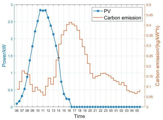
Figure 2.
The data for carbon emission intensity and photovoltaic (PV) output power.
4.2. Passive Collaborative Optimization Scheduling
- (1)
- Comparative Analysis of Evaluation Metrics under Different Scenarios
To verify the effectiveness of the HEMS framework based on NILM (Non-Intrusive Load Monitoring) and ultra-short-term forecasting, along with the carbon trading mechanism as a supplement to conventional HEMS, this paper sets up four comparative scenarios. Carbon emissions are used as the key evaluation metric for the optimization results. The optimization objectives for each scenario are shown in Table 2.
Table 2.
The setting of the optimization objective in different scenarios.
By comparing Scenario 2 with Scenario 1, the advantages of traditional HEMS in energy optimization management can be analyzed. Scenario 3 builds upon Scenario 2 by further considering user comfort. Scenario 4 introduces a carbon trading mechanism to evaluate its impact on electricity consumption optimization within HEMS and assess its advantages over other scenarios.
The computed results for each evaluation metric across the different scenarios are presented in Table 3. In Scenario 1, no energy management strategies are applied, resulting in the highest user comfort but also the highest electricity cost and carbon emissions. Scenario 2 is economically driven, considering dynamic electricity pricing to minimize electricity costs. However, it overlooks user preferences, leading to a significant drop in comfort. Scenario 3 balances electricity cost and user satisfaction; compared to Scenario 2, it significantly improves comfort while maintaining a lower electricity cost than Scenario 1, albeit higher than Scenario 2. Scenario 4 incorporates dynamic carbon emission factors and comprehensively considers all electricity-related indicators. Although the electricity cost is slightly higher than in Scenario 2, it achieves optimal performance in both user comfort and carbon emissions, yielding the lowest carbon output.
Table 3.
Evaluation indicators under different scenarios.
Compared to the other scenarios, the electricity optimization strategy in Scenario 4 more effectively encourages residents to participate in demand response programs and unlocks their potential for carbon reduction. It represents a mutually beneficial solution for both power grid operators and residential users.
- (2)
- Analysis of Energy Management Results under Different Scenarios
The operating time and power of each appliance under the electricity usage plans formulated by HEMS for different scenarios are shown in Figure 3. In these scenarios, the charging and discharging of energy storage systems and electric vehicles are directly controlled by HEMS, while the adjustable loads are only provided with suggestions regarding usage periods and power levels.
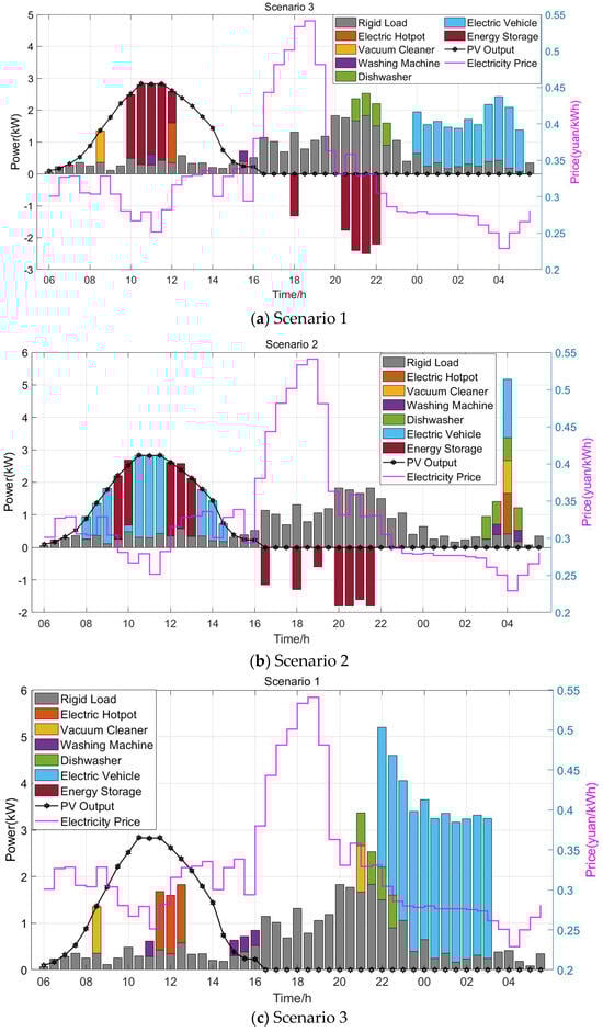
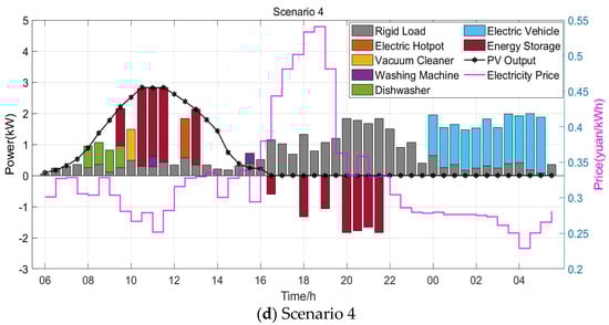
Figure 3.
Operating intervals and power of household appliances under different scenarios.
Scenario 1 serves as the baseline scenario, where neither user participation in demand response nor carbon trading is considered. In this case, HEMS does not engage in energy management. Load devices operate purely based on maximizing user satisfaction without any adjustments, and the energy storage system remains inactive. As a result, user comfort is maximized, but both daily electricity costs and carbon emissions are the highest.
Scenario 2 is driven by economic objectives and only considers the impact of dynamic electricity pricing on HEMS operating costs. This leads to the lowest electricity cost and overall cost among all scenarios. To effectively utilize the surplus electricity generated by PV systems and the advantage of low-price periods, the energy storage system and EV are fully charged between 08:00 and 14:30. During high-price periods (16:00–19:30), the storage system discharges to supply power to rigid loads. This shows that energy storage and demand response improve user flexibility and help users adjust their electricity usage behavior based on price signals, contributing positively to cost and carbon emission reductions. However, Scenario 2 neglects user habits, leading to a significant decrease in user comfort. Many appliances are scheduled at unreasonable times, such as using the vacuum cleaner or electric hotpot around 4 a.m., which does not align with typical user behavior. Compared to Scenario 1, user satisfaction in Scenario 2 drops by 55.7%, making it unsuitable for encouraging active user participation in demand response.
Scenario 3, based on NILM-inferred user behavior and optimized time intervals, considers both electricity cost and user satisfaction. Compared with Scenario 2, appliances in Scenario 3 operate within user-preferred periods—for example, the electric hotpot runs at 12:00, and the vacuum cleaner operates at 08:30. This results in a 105.41% improvement in user comfort, with only a slight increase in electricity cost and carbon emissions.
Scenario 4 represents the proposed strategy in this paper. Building upon Scenario 3, it incorporates both dynamic carbon emission factors and dynamic electricity pricing, optimizing for multiple objectives including electricity cost, user satisfaction, and carbon trading cost. Compared with Scenario 3, the introduction of the carbon emission factor results in more flattened scheduling of appliances and energy storage devices, avoiding clustering at specific time slots, which would otherwise cause load accumulation and sudden increases in carbon emissions. For instance, the dishwasher is scheduled during surplus PV generation periods rather than during peak power consumption times, and the EV charging times are more evenly distributed with power levels kept below 2 kW, preventing stepwise increases in carbon emissions. Compared to Scenario 3, Scenario 4 achieves a 0.21 yuan reduction in electricity costs (a 6.5% decrease), and a 0.28 kg reduction in carbon emissions (an 18.3% decrease), reaching the lowest carbon emissions among all four scenarios. User satisfaction also improves by 4.39%. Therefore, the optimization strategy in Scenario 4 is more conducive to guiding orderly residential participation in demand response and unlocking the potential for carbon reduction. It represents a mutually beneficial solution for both power grid enterprises and residential users.
- (3)
- Proactive Electricity Scheduling Based on Photovoltaic Output Forecasting
Traditional HEMS typically formulates a daily electricity usage plan based on day-ahead historical photovoltaic (PV) generation data. However, due to the influence of weather conditions such as solar irradiance intensity and cloud movement, PV output curves exhibit significant volatility, making it difficult for traditional HEMS to respond to short-term fluctuations in PV generation.
To address this issue, this paper adopts the GAT method. By using historical PV generation data and fine-grained meteorological parameters to train the prediction model, the model parameters are stored in the data center of the HEMS. During HEMS operation, real-time local weather station data is acquired and combined with PV generation data from the past 12 h to dynamically forecast PV output for the next hour. If the predicted PV output deviates significantly from historical values, the previously scheduled electricity usage plan will be adjusted accordingly.
Figure 4 shows a comparison among the historical PV output, predicted values, and actual PV output. As can be observed, compared to the historical PV data, the ultra-short-term forecasting method proposed in Paper 4 predicts a PV output peak of 2.4 kW, which is slightly lower than the actual peak of 2.5 kW and significantly lower than the historical peak value of 2.85 kW. Moreover, the predicted PV output drops sharply at 11:00 and approaches zero around 13:30, which is 30 min earlier than the actual value and 3 h earlier than the historical value. The RMSE between predicted and actual value is 0.1895 Kw. To provide proper context, we also compare GAT’s performance with two widely used baselines: Long Short-Term Memory (LSTM) [39] and Gated Recurrent Unit (GRU) models [40]. The LSTM model yields a RMSE of 0.2528 kW, and the GRU-based forecasting model achieves an RMSE of 0.2441 kW. The results show that GAT outperforms both models in terms of accuracy, demonstrating its effectiveness in capturing temporal and inter-appliance relationships.
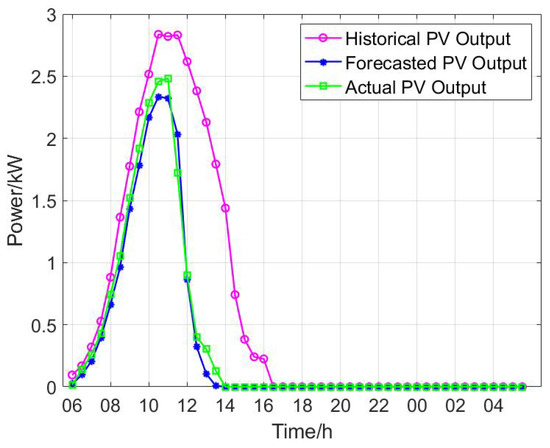
Figure 4.
Comparison of historical, predicted, and actual values of photovoltaic output power.
In this experiment, under the optimization objectives set in Scenario 4, an initial daily electricity usage plan is first formulated based on historical PV output data, referred to as the original usage plan. This plan is then adjusted using predicted PV output values to obtain the revised usage plan. The evaluation metrics under different PV data conditions are calculated and compared for both plans.
Three evaluation schemes are defined as follows:
- Scheme 1: The revised usage plan is executed, and evaluation metrics are calculated based on the predicted PV values. This scheme provides reference metrics used by HEMS at the time of scheduling.
- Scheme 2: The revised usage plan is executed, and evaluation metrics are calculated based on the actual PV values. This reflects the real electricity usage performance experienced by the user.
- Scheme 3: The original usage plan is executed, and evaluation metrics are calculated based on the actual PV values. This reflects the performance of the initial plan without correction.
The evaluation results for the three schemes are presented in Table 4. By comparing Scheme 1 and Scheme 2 in Table 4, and referring to Figure 4, it can be observed that due to the PV output in the prediction dropping approximately 30 min earlier than in the actual data, the electricity cost and carbon emission cost in Scheme 2 are slightly lower than those in Scheme 1. However, the differences between the two are minor, indicating that the PV prediction model used in this paper exhibits high accuracy. The revised electricity usage plan based on the predicted PV values closely aligns with the actual PV generation, demonstrating the practical effectiveness of the ultra-short-term forecasting method.
Table 4.
Evaluation indicators of different electricity consumption plans.
By comparing the evaluation indicators of the three schemes, it can be observed that in Scheme 3, where the original usage plan is followed despite the actual PV output decreasing earlier than the historical data, the highest level of user comfort is achieved. However, this also results in a significant increase in electricity drawn from the grid, leading to the highest electricity cost and carbon emission cost among the three schemes.
Compared with Scheme 3, Scheme 2 achieves a 16.1% reduction in electricity cost, a 32.7% reduction in carbon emission cost, and an 18.2% reduction in carbon emissions, while the user comfort decreases by only 1.2%. These results demonstrate that revising the original usage plan based on PV predictions can significantly reduce electricity costs and carbon emissions while maintaining a high level of user comfort.
The PV generation profiles and appliance operation schedules under the three schemes are illustrated in Figure 5. As shown in Figure 5c, in the original usage plan, the operation of the electric hot pot and the charging of the storage system were scheduled around 12:30, when PV generation was abundant in the historical data. However, due to sudden weather changes leading to earlier PV output decline, electricity from the grid was required to fulfill the original plan.
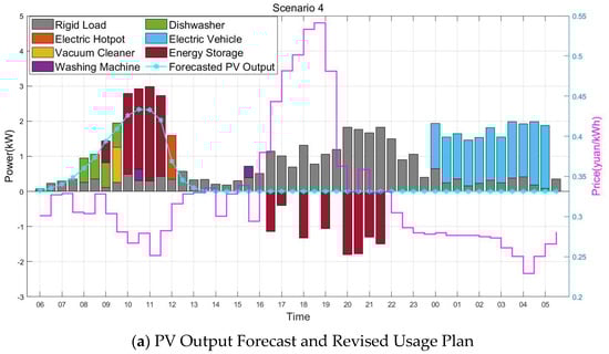
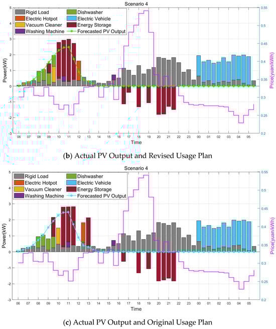
Figure 5.
The operating range and power diagram of electrical equipment under different schemes.
In contrast, Figure 5a,b show that, anticipating an early drop in PV output, the HEMS adjusted the schedule by shifting the operation of adjustable loads and the charging of the storage system to the 09:00–12:00 period, when PV output was still sufficient and electricity prices were relatively low. This ensured that during the 14:00–20:00 period, when PV generation was low and electricity prices were high, the energy stored earlier could be used to supply rigid loads, reducing the need for grid electricity and thus lowering costs and emissions.
In summary, integrating a PV output prediction model into the HEMS and dynamically adjusting the usage plan based on the predicted output enables effective reduction of both electricity costs and carbon emissions without compromising user engagement in energy optimization. This approach encourages the development of energy-saving and low-carbon electricity usage habits among residential users.
- (4)
- Proactive Electricity Scheduling Based on Load Forecasting
This experiment integrates historical electricity usage data with indoor and outdoor environmental parameters to analyze short-term fluctuations in electricity demand. Based on the GAT model, the total load is forecasted in a rolling manner. If there is a significant discrepancy between the predicted and historical load values, the original usage plan is adjusted according to the forecast. This involves pre-scheduling the charging of storage devices and adjusting the recommended usage times for flexible loads, while ensuring that user comfort is maintained and preventing excessive increases in electricity costs and carbon emissions.
In residential electricity usage, appliances such as air conditioners and water heaters, which are temperature-sensitive, experience sharp changes in load due to variations in ambient temperature. To more clearly demonstrate the effectiveness of the load forecasting-based usage plan adjustment method, this experiment only presents the power variations of the air conditioner and water heater from the load forecast results. Figure 6a,b show the historical power values of the air conditioner and water heater, as well as the total power consumption curve for both appliances.
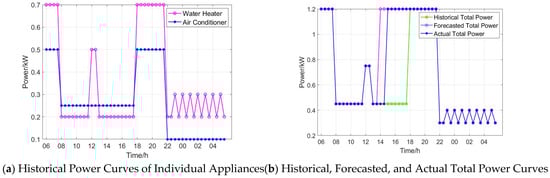
Figure 6.
Comparison of historical, predicted, and actual total power of air conditioners and water heaters.
As shown in Figure 6b, compared with the historical total power curve, the load forecasting method can predict the power surge of the air conditioner and water heater at 13:30, which is 1 h earlier than the actual value and 4 h earlier than the historical value. The RMSE between predicted and actual total power of air conditioners and water heaters is 0.1683 Kw. We also compare GAT’s performance with two widely used baselines: Long Short-Term Memory (LSTM) [39] and Gated Recurrent Unit (GRU) models [40]. The LSTM model yields a RMSE of 0.2528 kW, and the GRU-based forecasting model achieves an RMSE of 0.2441 kW. The results show that GAT outperforms both models in terms of accuracy, demonstrating its effectiveness in capturing temporal and inter-appliance relationships.
Next, the air conditioner and water heater are operated according to the forecasted power values, while other appliances follow the revised usage plan. The evaluation of this configuration is referred to as Scenario 4. In Scenario 5, the air conditioner and water heater operate based on their actual power values, while other appliances still follow the revised plan. In Scenario 6, the air conditioner and water heater operate based on their actual power values, but the other appliances follow the original usage plan.
Scenario 4 provides evaluation indicators for users as a reference when the original usage plan is adjusted based on the load forecast results. Scenario 5 reflects the actual performance under the revised usage plan, while Scenario 6 reflects the actual performance under the original usage plan. The evaluation results for these three scenarios are shown in Table 5.
Table 5.
Evaluation indicators before and after incorporating load forecasting.
As shown in Table 5, Scenario 6, which uses the original usage plan, fails to pre-charge the storage devices or adjust the operation periods of other appliances. Although it maintains the highest user comfort level, it requires additional electricity from the grid when the load increases earlier due to environmental factors, resulting in the highest electricity cost and carbon emissions. Compared with Scenario 6, Scenario 5 reduces electricity costs by 6.5%, carbon emission costs by 15.6%, and carbon emissions by 8.3%, while the user comfort level only drops by 3.4%. Comparing Scenario 4 and Scenario 5 in Table 5, and in combination with Figure 6, it can be observed that since the forecasted power of the air conditioner and water heater increases one hour earlier than the actual value, the electricity cost and carbon emission cost in Scenario 4 are slightly higher than in Scenario 5. However, the differences are minor, verifying the effectiveness of the GAT-based load forecasting model and the corresponding schedule adjustments.
The operation intervals and power levels of household appliances under different scenarios are shown in Figure 7. As seen in Figure 7c, when facing a sudden surge in total power demand, the original usage plan fails to effectively coordinate appliance usage. The battery is not fully charged during high PV output periods, leading to insufficient stored energy during the load surge period (14:00–18:00), and thus relying more heavily on electricity from the grid.
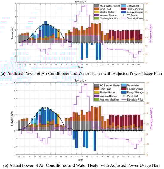
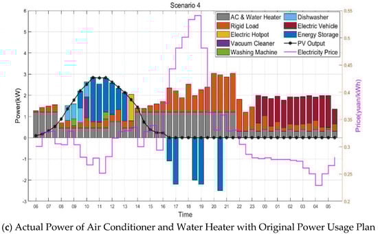
Figure 7.
Operation intervals and power curves of household appliances based on load forecasting and different planning methods.
In contrast, Figure 7a,b demonstrate that by integrating historical usage data and indoor/outdoor environmental parameters, the GAT model can predict upcoming power demand surges in advance. This enables timely schedule adjustments, thereby helping to reduce both electricity costs and carbon emissions.
Figure 8 illustrates the optimized scheduling outcomes for thermostatically controlled appliances, including air conditioners and water heaters. The results show that the water heater is scheduled to operate during several time intervals—particularly those aligning with peak demand for hot water—while its usage remains confined to mid-peak or off-peak electricity pricing periods, thus preserving user comfort and cost-efficiency. For the air conditioning unit, the system successfully stabilizes indoor temperatures around 26 °C, ensuring a high level of thermal comfort. These findings demonstrate that the proposed optimization strategy effectively synchronizes the operation of both devices, achieving a balance between user comfort and energy efficiency. Moreover, by responding dynamically to real-time electricity pricing, the strategy contributes to lowering overall energy expenses and reducing unnecessary power consumption.
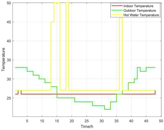
Figure 8.
The optimized scheduling outcomes for thermostatically controlled appliances.
Table 6 compares the performance of various algorithms across multiple evaluation metrics within Scheme 4. The results indicate that while the MILP algorithm yields superior optimization results compared to the GA approach, it is still outperformed by the proposed hybrid MILP + GA method. Nevertheless, MILP demonstrates a clear advantage in terms of computational efficiency, requiring significantly less solving time than the hybrid model. The MILP + GA approach, by contrast, offers a balanced compromise between solution quality and execution time, suggesting its greater practicality and robustness for deployment in real-world scenarios.
Table 6.
The performance of various algorithms across multiple evaluation. Metrics within Scheme 4.
5. Conclusions
Traditional Home Energy Management Systems (HEMS) face several limitations, including inadequate recognition of user behavior, inability to respond effectively to photovoltaic (PV) power fluctuations, and low accuracy in load forecasting, which hinder efficient energy optimization and real-time scheduling. To address these challenges, this paper proposes a short-term prediction-based HEMS optimization method aimed at enhancing the overall scheduling performance and responsiveness of the system. Firstly, the proposed method dynamically predicts PV output for the upcoming hour by leveraging historical PV generation data and real-time meteorological parameters. Simultaneously, it integrates historical household electricity consumption data and indoor/outdoor environmental conditions to build a total load forecasting model, thereby improving the system’s ability to anticipate demand fluctuations. Based on these predictions, a multi-objective optimization function is developed, incorporating electricity cost, user comfort, carbon emission cost, and grid load balance. An improved mixed-integer optimization algorithm is then employed to solve the problem. Simulation results demonstrate that the proposed algorithm outperforms benchmark approaches in reducing electricity costs, flattening the load curve, and cutting carbon emissions, while the slight reduction in user comfort remains within acceptable limits. In the proactive power scheduling strategy, the predicted PV output is used to iteratively adjust the daily usage plan and optimize the charge/discharge strategy of the energy storage system, effectively reducing reliance on the grid during high-tariff periods. In the load-forecast-driven scheduling strategy, anticipated load surges—such as those caused by air conditioners and water heaters—are detected in advance, enabling timely adjustments that further reduce both electricity costs and carbon emissions. In conclusion, the proposed short-term prediction-driven proactive HEMS optimization method significantly enhances economic performance, environmental sustainability, and system responsiveness, all while maintaining acceptable levels of user comfort, making it highly applicable and valuable for future smart home energy systems.
Author Contributions
Conceptualization, S.L. and Z.H.; methodology, S.L. and K.Z.; software, S.L.; validation, S.L.; formal analysis, S.L. and W.G.; writing—original draft preparation, Z.X.; writing—review and editing, Z.X., X.L. and Z.H.; supervision, Z.H. All authors have read and agreed to the published version of the manuscript.
Funding
This work was funded by the General Program of National Natural Science Foundation of China (Grant No. 52177083 and 62001166), and by Major Science and Technology Projects in Hebei Province (Grant No. 23281701Z).
Data Availability Statement
The original contributions presented in this study are included in the article. Further inquiries can be directed to the corresponding author.
Conflicts of Interest
The authors declare no conflicts of interest.
Abbreviations
The following abbreviations are used in this manuscript:
| SHEM | Smart home energy management |
| NILM | Non-intrusive load monitoring |
| AI | Artificial intelligence |
| IoT | Internet of Things |
| MILP | Mixed-integer linear programming |
| GA | Genetic algorithm |
| DR | Demand response |
| TOU | Time-of-use pricing |
| SOC | State of charge |
| PV | Photovoltaic |
| RTP | Real-time pricing |
| EV | Electric vehicle |
| B&B | Branch and bound |
| LP | Linear programming |
| MDP | Markov decision process |
| LSTM | Long short-term memory |
| HVAC | Heating, ventilation, and air conditioning |
| CNY | Chinese yuan |
References
- Zhou, B.; Li, W.; Chan, K.W.; Cao, Y.; Kuang, Y.; Liu, X.; Wang, X. Smart home energy management systems: Concept, configurations, and scheduling strategies. Renew. Sustain. Energy Rev. 2016, 61, 30–40. [Google Scholar] [CrossRef]
- Badar, A.Q.H.; Anvari-Moghaddam, A. Smart home energy management system–A review. Adv. Build. Energy Res. 2022, 16, 118–143. [Google Scholar] [CrossRef]
- Talebi, H.; Kazemi, A.; Shakouri, H.; Kocaman, A.S.; Caldwell, N. An integrated price-and incentive-based demand response program for smart residential buildings: A robust multi-objective model. Sustain. Cities Soc. 2024, 113, 105664. [Google Scholar] [CrossRef]
- Guo, C. Research on Power Load Forecasting and Supply-Demand Benefit Coordination Optimization Under Demand Response. Ph.D. Thesis, Shenyang Agricultural University, Shenyang, China, 2018. [Google Scholar]
- Kanakadhurga, D.; Prabaharan, N. Smart home energy management using demand response with uncertainty analysis of electric vehicle in the presence of renewable energy sources. Appl. Energy 2024, 364, 123062. [Google Scholar] [CrossRef]
- Hou, H.; Gan, M.; Wu, X.; Xie, K.; Fan, Z.; Xie, C.; Shi, Y.; Huang, L. Real-Time Low-Carbon Optimization Management of Household Energy Considering Carbon Trading Under Non-Predictive Mechanisms. Power Syst. Technol. 2023, 47, 1066–1077. [Google Scholar]
- Liu, Y.; Li, D.; Pei, H.; Liu, K.; Li, Y.; Yang, L. Short-term load prediction method for power distributing method based on back-propagation neural network. In Proceedings of the 2017 12th IEEE Conference on Industrial Electronics and Applications (ICIEA), Siem Reap, Cambodia, 18–20 June 2017; IEEE: New York, NY, USA, 2017; pp. 881–886. [Google Scholar]
- Narayan, A.; Hipel, K.W. Long short term memory networks for short-term electric load forecasting. In Proceedings of the 2017 IEEE International Conference on Systems, Man, and Cybernetics (SMC), Banff, AB, Canada, 5–8 October 2017; IEEE: New York, NY, USA, 2017; pp. 2573–2578. [Google Scholar]
- Zhu, R.; Liao, W.; Wang, Y. Short-term prediction for wind power based on temporal convolutional network. Energy Rep. 2020, 6, 424–429. [Google Scholar] [CrossRef]
- Bilgili, M.; Pinar, E. Gross electricity consumption forecasting using LSTM and SARIMA approaches: A case study of Türkiye. Energy 2023, 284, 128575. [Google Scholar] [CrossRef]
- Bu, X.; Wu, Q.; Zhou, B.; Li, C. Hybrid short-term load forecasting using CGAN with CNN and semi-supervised regression. Appl. Energy 2023, 338, 120920. [Google Scholar] [CrossRef]
- Chiu, M.-C.; Hsu, H.-W.; Chen, K.-S.; Wen, C.-Y. A hybrid CNN-GRU based probabilistic model for load forecasting from individual household to commercial building. Energy Rep. 2023, 9, 94–105. [Google Scholar] [CrossRef]
- Farrokhifar, M.; Momayyezi, F.; Sadoogi, N.; Safari, A. Real-time based approach for intelligent building energy management using dynamic price policies. Sustain. Cities Soc. 2018, 37, 85–92. [Google Scholar] [CrossRef]
- Qureshi, K.N.; Alhudhaif, A.; Hussain, A.; Iqbal, S.; Jeon, G. Trust aware energy management system for smart homes appliances. Comput. Electr. Eng. 2022, 97, 107641. [Google Scholar] [CrossRef]
- Jaradat, A.; Lutfiyya, H.; Haque, A. Smart home energy visualizer: A fusion of data analytics and information visualization. IEEE Can. J. Electr. Comput. Eng. 2022, 45, 77–87. [Google Scholar] [CrossRef]
- Ajao, A.; Luo, J.; Liang, Z.; Alsafasfeh, Q.H.; Su, W. Intelligent home energy management system for distributed renewable generators, dispatchable residential loads and distributed energy storage devices. In Proceedings of the 2017 8th International Renewable Energy Congress (IREC), Amman, Jordan, 21–23 March 2017; IEEE: New York, NY, USA, 2017; pp. 1–6. [Google Scholar]
- Luo, F.; Xu, Z.; Meng, K.; Dong, Z.Y. Optimal operation scheduling for microgrid with high penetrations of solar power and thermostatically controlled loads. Sci. Technol. Built Environ. 2016, 22, 666–673. [Google Scholar] [CrossRef]
- Akram, A.S.; Abbas, S.; Khan, M.A.; Athar, A.; Ghazal, T.M.; Al Hamadi, H. Smart energy management system using machine learning. Comput. Mater. Contin. 2024, 78, 959–973. [Google Scholar] [CrossRef]
- Yang, Y.; Wang, S. Resilient residential energy management with vehicle-to-home and photovoltaic uncertainty. Int. J. Electr. Power Energy Syst. 2021, 132, 107206. [Google Scholar] [CrossRef]
- Yousefi, M.; Hajizadeh, A.; Soltani, M.N.; Hredzak, B. Predictive home energy management system with photovoltaic array, heat pump, and plug-in electric vehicle. IEEE Trans. Ind. Inform. 2020, 17, 430–440. [Google Scholar] [CrossRef]
- Rastegar, M.; Fotuhi-Firuzabad, M.; Zareipour, H.; Moeini-Aghtaieh, M. A probabilistic energy management scheme for renewable-based residential energy hubs. IEEE Trans. Smart Grid 2016, 8, 2217–2227. [Google Scholar] [CrossRef]
- Jamil, M.; Mittal, S. Hourly load shifting approach for demand side management in smart grid using grasshopper optimisation algorithm. IET Gener. Transm. Distrib. 2020, 14, 808–815. [Google Scholar] [CrossRef]
- Sarker, E.; Seyedmahmoudian, M.; Jamei, E.; Horan, B.; Stojcevski, A. Optimal management of home loads with renewable energy integration and demand response strategy. Energy 2020, 210, 118602. [Google Scholar] [CrossRef]
- Huang, Z.; Wang, F.; Lu, Y.; Chen, X.; Wu, Q. Optimization model for home energy management system of rural dwellings. Energy 2023, 283, 129039. [Google Scholar] [CrossRef]
- Carli, R.; Dotoli, M. Decentralized control for residential energy management of a smart users’ microgrid with renewable energy exchange. IEEE/CAA J. Autom. Sin. 2019, 6, 641–656. [Google Scholar] [CrossRef]
- Hu, R.; Zhou, K.; Yin, H. Reinforcement learning model for incentive-based integrated demand response considering demand-side coupling. Energy 2024, 308, 132997. [Google Scholar] [CrossRef]
- Dey, B.; Sharma, G.; Bokoro, P.N.; Dutta, S. An intelligent incentive-based demand response program for exhaustive environment constrained techno-economic analysis of microgrid system. Sci. Rep. 2025, 15, 894. [Google Scholar] [CrossRef] [PubMed]
- Siddiquee, S.S.; Agyeman, K.A.; Bruton, K.; Howard, B.; O’Sullivan, D.T. A data-driven assessment model for demand response participation benefit of industries. In Proceedings of the 2022 IEEE Texas Power and Energy Conference (TPEC), College Station, TX, USA, 28 February–1 March 2022; IEEE: New York, NY, USA, 2022; pp. 1–6. [Google Scholar]
- Zhang, Y.; Ge, X.; Li, M.; Li, N.; Wang, F.; Wang, L.; Sun, Q. Demand response potential day-ahead forecasting approach based on LSSA-BPNN considering the electricity-carbon coupling incentive effects. IEEE Trans. Ind. Appl. 2024, 60, 4505–4516. [Google Scholar] [CrossRef]
- Chen, J.; Hu, Z.; Chen, J. Optimal Dispatch of Integrated Energy Systems Considering Stepwise Carbon Trading and Flexible Supply-Demand Dual Response. High Volt. Eng. 2021, 47, 3094–3104. [Google Scholar]
- Zeng, A.D.; Zou, Y.H.; Hao, S.P. Integrated Demand Response Strategy for Industrial Users in Park Considering Stepwise Carbon Trading Mechanism. High Volt. Eng. 2022, 48, 4352–4361. [Google Scholar]
- Han, Y.; Yu, S.C.; Li, L.Y.; Hou, Y.; Li, Q.; Chen, R. Low-Carbon Economic Configuration Method for Wind-Solar-Hydrogen-Storage Microgrid Considering Stepwise Carbon Trading Mechanism. High Volt. Eng. 2022, 48, 2523–2533. [Google Scholar]
- Javadi, M.S.; Nezhad, A.E.; Nardelli, P.H.; Gough, M.; Lotfi, M.; Santos, S.; Catalão, J.P. Self-scheduling model for home energy management systems considering the end-users discomfort index within price-based demand response programs. Sustain. Cities Soc. 2021, 68, 102792. [Google Scholar] [CrossRef]
- De Vizia, C.; Patti, E.; Macii, E.; Bottaccioli, L. A win-win algorithm for learning the flexibility of aggregated residential appliances. IEEE Access 2021, 9, 150495–150507. [Google Scholar] [CrossRef]
- Stanescu, D.; Enache, F.; Popescu, F. Smart Non-Intrusive Appliance Load-Monitoring System Based on Phase Diagram Analysis. Smart Cities 2024, 7, 1936–1949. [Google Scholar] [CrossRef]
- Ioana, C.; Digulescu, A.; Serbanescu, A.; Candel, I.; Birleanu, F.M. Recent advances in non-stationary signal processing based on the concept of recurrence plot analysis. In Translational Recurrences: From Mathematical Theory to Real-World Applications; Springer: Cham, Switzerland, 2014; pp. 75–93. [Google Scholar]
- Nutakki, M.; Mandava, S. Resilient data-driven non-intrusive load monitoring for efficient energy management using machine learning techniques. EURASIP J. Adv. Signal Process. 2024, 2024, 62. [Google Scholar] [CrossRef]
- Liu, S.; Xie, Z.; Hu, Z. A Distributed Non-Intrusive Load Monitoring Method Using Karhunen–Loeve Feature Extraction and an Improved Deep Dictionary. Electronics 2024, 13, 3970. [Google Scholar] [CrossRef]
- Liu, Y.; Wang, J. Long Short-Term Memory Based Refined Load Prediction Utilizing Non Intrusive Load Monitoring. In Proceedings of the 2021 IEEE Power & Energy Society General Meeting (PESGM), Washington, DC, USA, 26–29 July 2021; IEEE: New York, NY, USA, 2021; pp. 1–5. [Google Scholar]
- Putrada, A.G.; Alamsyah, N.; Pane, S.F.; Fauzan, M.N. Gru-mf: A novel appliance classification method for non-intrusive load monitoring data. In Proceedings of the 2022 IEEE International Conference on Communication, Networks and Satellite (COMNETSAT), Solo, Indonesia, 3–5 November 2022; IEEE: New York, NY, USA, 2022; pp. 200–205. [Google Scholar]
Disclaimer/Publisher’s Note: The statements, opinions and data contained in all publications are solely those of the individual author(s) and contributor(s) and not of MDPI and/or the editor(s). MDPI and/or the editor(s) disclaim responsibility for any injury to people or property resulting from any ideas, methods, instructions or products referred to in the content. |
© 2025 by the authors. Licensee MDPI, Basel, Switzerland. This article is an open access article distributed under the terms and conditions of the Creative Commons Attribution (CC BY) license (https://creativecommons.org/licenses/by/4.0/).