Abstract
Energy storage plays an essential role in stabilizing fluctuations in renewable energy sources such as wind and solar, enabling surplus electricity retention, and delivering dynamic frequency regulation. However, relying solely on a single form of storage often proves insufficient due to constraints in performance, capacity, and cost-effectiveness. To tackle frequency regulation challenges in remote desert-based renewable energy hubs—where traditional power infrastructure is unavailable—this study introduces a planning framework for an electro-hydrogen energy storage system with grid-forming capabilities, designed to supply both inertia and frequency response. At the system design stage, a direct current (DC) transmission network is modeled, integrating battery and hydrogen storage technologies. Using this configuration, the capacity settings for both grid-forming batteries and hydrogen units are optimized. This study then explores how hydrogen systems—comprising electrolyzers, storage tanks, and fuel cells—and grid-forming batteries contribute to inertial support. Virtual inertia models are established for each technology, enabling precise estimation of the total synthetic inertia provided. At the operational level, this study addresses stability concerns stemming from renewable generation variability by introducing three security indices. A joint optimization is performed for virtual inertia constants, which define the virtual inertia provided by energy storage systems to assist in frequency regulation, and primary frequency response parameters within the proposed storage scheme are optimized in this model. This enhances the frequency modulation potential of both systems and confirms the robustness of the proposed approach. Lastly, a real-world case study involving a 13 GW renewable energy base in Northwest China, connected via a ±10 GW HVDC export corridor, demonstrates the practical effectiveness of the optimization strategy and system configuration.
1. Introduction
Under the broader context of the green energy transition, DC power transmission has emerged as a critical method for efficient energy transfer and rational distribution. Particularly in remote regions such as deserts, plateaus, and offshore areas, where large-scale renewable energy bases are located, DC transmission plays an essential role in optimizing the national energy layout and improving the utilization efficiency of clean energy [1]. However, these bases typically lack the support of conventional power sources and exhibit weak AC system characteristics. The stochastic and fluctuating nature exacerbates the challenge of maintaining frequency stability and security [2,3]. Consequently, improving frequency stability under limited inertia support has become a pressing issue.
Electrochemical energy storage (EES) systems offer fast frequency response and strong regulation capabilities, but their lifespan is limited by frequent charge–discharge cycles, resulting in higher daily investment costs. In contrast, hydrogen energy storage (HES) systems exhibit relatively weaker frequency response speed and regulation capability. Compared with single-type storage, a hybrid electrochemical–hydrogen storage system can balance high capacity, economic feasibility, and frequency security in renewable energy bases.
Frequency stability mainly concerns the convergence of the system’s quasi-steady-state frequency after disturbances, while frequency security focuses on whether dynamic frequency variations remain within equipment-specified thresholds. Safety indicators such as the RoCoF and maximum frequency deviation are typically used for assessment [4,5]. Power electronic devices like converters in renewable energy bases are highly sensitive to frequency fluctuations, making both stability and security essential [6]. Given their advantages in inertia and frequency support, advanced EES and HES systems can significantly improve disturbance resilience. Thus, developing a planning and configuration strategy that fully considers the inertia and frequency support capacities of EES and HES is vital for the secure and stable operation of renewable energy bases.
EESs are typically classified according to their control methods into either grid-forming or grid-following types. Grid-forming energy storage mimics the rotational inertia of synchronous generators via power electronic converters [7,8], offering fast frequency response capabilities and improving overall power system stability [9,10,11,12]. Researchers worldwide have proposed various grid-forming control strategies, including virtual oscillator control (VOC) [13], droop control [14], and virtual synchronous generator (VSG) control [15,16].
Among these, the VSG method is widely adopted in engineering practice due to its fast power response and minimal constraints [17,18]. For instance, reference [19] proposed an adaptive inertia-damping composite control method to address the inadequacy of traditional constant–parameter and adaptive inertia methods in considering damping effects, using interleaved control to improve frequency stability. Reference [20] introduced a linear quadratic optimal control approach for dynamically allocating VSG virtual inertia and damping, effectively suppressing oscillations in active power and frequency while optimizing energy storage capacity. In [21], a decoupled Reactive Power Feedforward (RPFF) control strategy under the MPME framework was proposed to enhance VSG system stability and robustness, with experimental validation of the model and control scheme. Furthermore, ref. [22] developed a method for VSG-based AC microgrids by modeling the nonlinear dynamics and improving frequency regulation performance through nonlinear dynamic analysis.
Hydrogen energy storage, known for its broad power regulation range and large-scale adaptability, is widely used in renewable energy bases. It effectively smooths wind and solar fluctuations and reduces curtailment [23,24]. Moreover, HES can emulate virtual synchronous generators to provide inertia support, enhancing the system’s frequency regulation capability. Reference [25] proposed a hydrogen-based solution to mitigate renewable energy intermittency and improve frequency stability. Power system analysis validated its effectiveness. Reference [26] developed a coordinated control strategy for hydrogen-powered microgrids using a disturbance-rejection model predictive controller (MPC), while [27] proposed a data-driven MPC for coordinating HESS and distributed generators in islanded microgrids, demonstrating effective real-time frequency regulation. However, these studies focused on frequency response under fixed power conditions without considering how capacity configuration affects the frequency support of EES and HESS.
Recently, several studies have explored storage configuration optimization to enhance frequency stability in renewable energy bases. Reference [28] addressed the lack of conventional units in desert-based renewable energy bases and proposed a grid-forming energy storage planning method without conventional generation support. This study derived a configuration scheme that meets system requirements, which focus solely on capacity planning. Reference [29] proposed a system strength-constrained optimal planning method based on grid-forming storage to address system strength reduction caused by high renewable penetration, which considers frequency support in isolation. Case verified the effectiveness and efficiency of the method across different scenarios.
While these studies leverage grid-forming control for frequency regulation, they do not consider the cooperative use of EES and HES for frequency support, nor do they optimize virtual inertia time constants or primary frequency coefficients, which are often fixed. Fixed frequency support parameters may limit the dynamic adaptability of grid-forming storage across different generation and DC transmission conditions, leading to increased storage capacity requirements and higher costs. This paper proposes a tightly coupled bi-level model that integrates frequency security constraints into storage sizing decisions.
2. Framework of the Planning and Configuration Model for Grid-Forming Electrochemical and HESS in Renewable Energy Bases
The proposed bi-level planning framework for grid-forming EES and HESS in renewable energy bases, which incorporates inertia response and primary frequency regulation parameter optimization, is illustrated in Figure 1. The upper layer focuses on economic planning, optimizing the rated power and capacity of the grid-forming battery and hydrogen systems under typical renewable generation scenarios and DC transmission constraints. The lower layer models the system’s dynamic frequency response, evaluating three frequency security indicators (RoCoF, maximum frequency deviation, and quasi-steady-state deviation) and optimizing primary frequency regulation coefficients and virtual inertia time constants. These two layers are coupled through an iterative feedback loop: configuration decisions from the upper layer inform the dynamic response model in the lower layer, while performance feedback guides adjustments to capacity and control parameters.
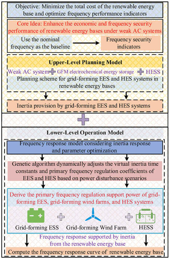
Figure 1.
Planning framework for grid-forming electricity HESS in renewable energy base.
2.1. Inertia Model of the HESS
To ensure frequency stability without conventional power support and enhance PV accommodation capability, a HESS comprising an electrolyzer, hydrogen storage tank, and hydrogen fuel cell is deployed within the renewable energy base, providing inertia and frequency regulation support. The inertia support and frequency response mechanisms of the HESS in the renewable energy base are illustrated in Figure 2.
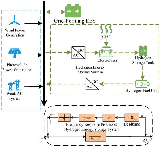
Figure 2.
Inertia support and frequency response process of the hydrogen storage system in the new energy base.
In Figure 2, represents the active power increment of the HESS; denotes the frequency deviation at time t; denotes the primary frequency regulation coefficient of the HESS; and indicates the system power imbalance.
2.2. Comparison of Electrochemical and Hydrogen Energy Storage in Grid-Forming Control of Renewable Energy Bases
The construction and operation of renewable energy bases face numerous challenges, particularly the deterioration of frequency security indicators due to the lack of support from conventional power sources. To address this pressing issue, this paper proposes a coordinated utilization strategy of EES and HESS. By implementing a collaborative grid-forming control approach that integrates both EES and HESS, the frequency security of renewable energy bases can be significantly enhanced. This strategy improves the grid’s disturbance rejection capability, thereby providing robust support for the stab operation.
Electrochemical energy storage (EES) systems exhibit rapid frequency response capabilities and can provide substantial inertia support to renewable energy bases over short time scales, thereby demonstrating strong frequency regulation performance. Particularly during fluctuations in renewable power generation, EES can swiftly respond to grid frequency deviations, preventing frequency indices from exceeding operational limits. However, due to the inherent uncertainty in PW output in large-scale renewable energy bases.
In contrast, HESS systems offer higher energy density and longer storage duration, enabling them to deliver more sustained inertia responses in renewable energy bases. Although HES provides weaker inertia support compared to EES, it benefits from a longer service life and consequently lower unit investment cost. Furthermore, HES systems can utilize fuel cells to convert stored hydrogen into electricity, offering stable support for the direct current (DC) power transmission from renewable energy bases.
Therefore, EES and HES can complement each other in the context of frequency regulation within renewable energy bases, leveraging their respective strengths. EES is more suitable for fast response, short-term frequency modulation, and inertia support, whereas HES provides reliable support for large-scale energy storage and long-duration frequency regulation. By optimally coordinating and configuring both EES and HESS, the number of EES charge–discharge cycles can be reduced, prolonging battery life and enhancing both the frequency security and economic efficiency of renewable energy base operations.
2.3. Inertia and Frequency Response of HESS in Renewable Energy Bases
Unlike traditional power systems that rely on synchronous machines for frequency regulation, renewable energy bases lacking conventional power sources utilize grid-forming control strategies to perform frequency regulation. During the inertia response phase, HES systems can provide inertia support similar to that of thermal power units, thereby mitigating frequency fluctuations. Subsequently, through grid-forming control, HES systems can also participate in active power regulation to accomplish primary frequency control tasks.
As shown in Figure 3, the interval corresponds to the inertia response phase, while represents the frequency regulation phase. Prior to , the system operates at the nominal frequency . At , a power deficit triggers a rapid frequency decline. The HESS inertia response is activated immediately, arresting the frequency drop at the nadir by . Frequency recovery initiates thereafter, concluding with stabilization at . The governing equation for this process is as follows:
where represents the system inertia constant; represents the active power increment of the HESS at time ; indicates the system power imbalance at time ; and is the damping coefficient.
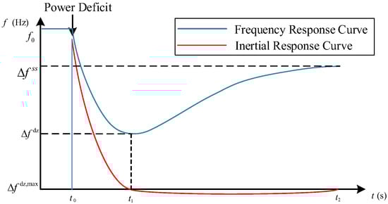
Figure 3.
Inertia and frequency response process of hydrogen energy storage system in new energy base.
2.4. Modeling and Operational Constraints of the HESS
- (1)
- Modeling and Operational Constraints of HESS:where and represent the electrical input power and hydrogen production power; denotes the electrolyzer efficiency; and are the minimum and maximum allowable input powers; and and denote the maximum permissible power increase and decrease, respectively.
- (2)
- The hydrogen storage tank model encompasses three operational constraints: storage capacity limits, hydrogen inflow/outflow rate constraints, and output power boundaries, formulated as follows:where is the hydrogen storage level of the tank at time t; and are the hydrogen input and output powers of the tank at time t; and are the charging and discharging efficiencies of the hydrogen tank; and denote the minimum and maximum hydrogen storage capacity; and represent the minimum and maximum hydrogen charging power; and represent the minimum and maximum hydrogen discharging power; and is a binary variable indicating the tank’s operational mode, where 1 corresponds to charging mode and 0 to discharging mode.
- (3)
- The hydrogen fuel cell model includes power conversion constraints, input power constraints, and ramping constraints:where and represent the output electrical power and input hydrogen power of the HFC; denotes the conversion efficiency of the HFC; and are the upper and lower limits of the HFC’s input power; and and are the upper and lower limits of the HFC’s ramping power.
2.5. Virtual Inertia Model of the Hydrogen Energy Storage System
Since photovoltaic power plants lack rotating components, they cannot independently provide inertia support to renewable energy bases. Hydrogen energy storage systems can participate in the frequency regulation process of renewable energy bases by emulating virtual synchronous generators. Therefore, virtual inertia modeling can be performed by treating the PV power plant and HESS as an integrated entity.
The operational load states of the HESS are expressed as follows:
The virtual inertia time constant of the HESS is as follows:
The virtual inertia provided by the HESS is as follows:
where is the load state of the HESS at time t; is the per-unit base power; and is the charge/discharge rate of the HESS.
2.6. Frequency Indicator and Frequency Regulation Parameter Optimization
2.6.1. Frequency Indicators
Frequency security is critically important for renewable energy bases. Frequency security primarily refers to whether the dynamic frequency variations at each time instance following a disturbance meet the safety requirements of grid frequency indices for equipment. To this end, this study applies discretization to each time instance, with a discretization period of 6 s and a time step of 0.2 s. The considered frequency security indices include the following:
- (1)
- RoCoFwhere represents the security thresholds for the RoCoF at time ’ represents the system nominal frequency; represents the disturbance power imposed at time t; and represents the minimum inertia requirement.
- (2)
- Maximum Frequency Deviationwhere is the frequency deviation at the g-th time step within time interval t.
- (3)
- Quasi-Steady-State Frequency Deviation
2.6.2. Frequency Regulation Parameter Optimization
- (1)
- Constraint on primary frequency coefficient of the HESSwhere is the primary frequency regulation coefficient of the hydrogen energy storage system at time t, and and are its lower and upper bounds, respectively.
- (2)
- Constraint on Virtual Inertia Time Constant of the HESSwhere and are the corresponding bounds.
- (3)
- Constraint on Primary Frequency Coefficient of Grid-Forming EESwhere and are its lower and upper bounds.
- (4)
- Constraint on Virtual Inertia Time Constant of Grid-Forming EESwhere and are the corresponding bounds.
3. Planning of Grid-Forming Electrochemical and Hydrogen Energy Storage Systems Considering Inertia Response and Parameter Optimization
3.1. Configuration Model of Grid-Forming Electrochemical and HESS
3.1.1. Planning Objective Function
3.1.2. Modeling of DC Operation Mode
- (1)
- DC Operation Constraints
DC Power Export Transmission Range Constraint
where is the DC export power, and and , respectively, represent the lower and upper bounds of DC transmission power.
- (2)
- Adjacent Time-Step Ramping Power Constraints for DC Lines
- (3)
- Minimum Duration Constraint for Constant DC Power Operation
This constraint limits the continuous operation time of DC equipment to ensure stab performance during prolonged operation.
where represents minimum time intervals allowed between power adjustments.
- (4)
- Maximum Daily Adjustment Count Constraint for DC Power
3.1.3. Typical Scenario-Based Operational
- (1)
- Power Balance Constraint
The constraint is the fundamental requirement that renewable energy base-planning schemes must satisfy:
where represents the actual output of the PW at time t; represents actual output of the PV plant; and and , respectively, represent the discharging and charging power of the grid-forming EES at time t.
- (2)
- Weak AC Grid Support Power Constraint
The support power provided by the weak AC grid must operate within specified limits:
where and , respectively, represent the lower and upper bounds of the support power provided by the weak AC grid.
- (3)
- Renewable Energy Output Constraints
The available maximum output and forecast power of renewable energy must satisfy Equations (29) and (30).
- (4)
- The operational constraints of the grid-forming EES include discharging/charging power constraints (33) and (34); charging/discharging state variable constraint (35); and capacity constraints (36)–(39).
- (5)
- Constraints of electrolyzer, hydrogen tank, and fuel cell (see Equations (4)–(6)).
3.1.4. Inertia Support from Renewable Energy Base
Total equivalent inertia of a renewable energy base can be expressed as follows:
where is virtual inertia time constant of the wind farm at time t; is the total inertia of the grid-forming wind farm at time t; and represents the rated power of grid-forming wind farm.
3.1.5. Power and Capacity Constraints of Transient Process Equipment
When grid-forming EES participates in frequency regulation, higher settings of its primary frequency regulation parameters enhance its frequency support capability. However, during large disturbances, excessive parameter settings may cause the EES equipment to exceed safety limits for power or capacity during transient processes, compromising device integrity or even leading to safety risks. Therefore, transient-state power and capacity constraints of the EES equipment must be considered in parameter optimization.
where represents the total frequency regulation power provided by the EES at the g-th time step after a disturbance at time t; is the primary frequency regulation power of the grid-forming EES at the g-th time step after a disturbance at time t; and represents the maximum charge/discharge rate of grid-forming EES.
3.2. Frequency Response Layer Model of Renewable Energy Base Considering Inertia Response and Primary Frequency Regulation Optimization
3.2.1. Modeling of Frequency Response Layer for Renewable Energy Base
This paper establishes the frequency response model of the renewable energy base, as shown in Figure 4.
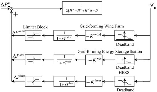
Figure 4.
Frequency response control model of new energy base.
3.2.2. Objective Function of Frequency Response Layer
3.2.3. Primary Frequency Regulation Power Support
- (1)
- Constraints of Grid-Forming Wind Farm
Primary Frequency Adjustment Power
Active Power Reserve Constraints for Primary Frequency Regulation
where and denote the primary frequency regulation power and actual regulation power of the grid-forming wind farm at the g-th time step after a disturbance at time t. and represent the first--order inertia time constant and primary frequency regulation coefficient during the PFR phase of the grid-forming wind farm.
- (2)
- Grid-Forming Electrochemical Energy Storage Station
Primary Frequency Adjustment Power of Grid-Forming Electrochemical Storage
- (3)
- HESS
Primary Frequency Adjustment Power of Hydrogen Energy Storage
where represent the first-order inertia time constant.
3.2.4. Discretized Frequency Security Indicators
After discretizing the three frequency indicators, the power imbalance at the g-th step following a disturbance at time t is obtained, from which the RoCoF and the corresponding frequency deviation at the g-th step can be derived.
where is the power imbalance at the g-th time step following a disturbance at time t.
- (1)
- RoCoF
- (2)
- Frequency Deviation
- (3)
- Quasi-Steady-State Frequency Deviation
- (4)
- Frequency Indicator Constraints
4. Model Solution
Due to the presence of numerous nonlinear components in the lower-level frequency response model, solving the system equations becomes computationally challenging. Genetic algorithms, known for their strong adaptability to nonlinear optimization problems, are capable of effectively avoiding local optima during the search process. Therefore, this study employs a GA to solve it. The population size is set to 200, the crossover rate is 0.8, the mutation rate is 0.01, and the stopping criterion is the maximum number of iterations reaching 500.
The solution procedure is illustrated in Figure 5.
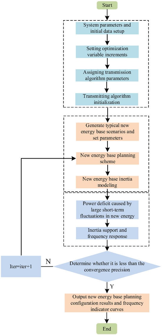
Figure 5.
Optimal allocation and frequency response model solution process for new energy bases.
- Step 1:
- System parameters and initial data setup: Set various economic parameters, frequency modulation control parameters, and raw data for wind and solar power generation.
- Step 2:
- Setting optimization variable increments: This includes the boundary for the rated power of energy storage, rated capacity of energy storage, rated power of electrolyzers, rated capacity of hydrogen storage tanks, and rated power of hydrogen fuel cells, as well as the boundaries for virtual inertia time constants of energy storage and hydrogen storage, and primary frequency modulation coefficients.
- Step 3:
- Assigning transmission algorithm parameters: This includes population size, maximum generations, crossover rate, elite individual count, mutation rate, and convergence precision.
- Step 4:
- Transmitting algorithm initialization: Randomly generate an initial population and convert the frequency regulation index objective function at the operation level into an economic index, then add it to the planning-level objective function and penalty terms to set the genetic algorithm’s fitness function.
- Step 5:
- Generation of Typical Scenarios for the New Energy Base: Typical wind and solar power output scenarios were generated for new energy bases in the Northwest region. Initial parameters were configured, including algorithm parameters, economic parameters, and control parameters.
- Step 6:
- Optimization of New Energy Base-Planning Scheme: Based on this, the configurations for grid-forming-type battery energy storage systems and HESS were determined.
- Step 7:
- Virtual Inertia Modeling of the New Energy Base: Virtual inertia models were developed for grid-forming battery storage, grid-forming wind farms, and hydrogen storage systems based on Equations (7), (38), and (39). The total virtual inertia of the new energy base was then calculated using the previously determined configuration results.
- Step 8:
- Power Deficiency Caused by Short-Term Large Disturbances: To simulate a major disturbance, 10% of the historical forecasted output of new energy was used as the disturbance value.
- Step 9:
- Inertia Support and Frequency Response: To enhance grid stability, the response characteristics of grid-forming battery systems, wind farms, and hydrogen-based storage were configured. This step aimed to fine-tune key performance indicators, ensuring each technology contributed effectively to overall frequency regulation.
- Step 10:
- Convergence Check: If the difference between the current fitness function value and the optimal value was smaller than the set convergence threshold, the planning configuration results of the new energy base and its frequency response curves were output. If the difference exceeded the threshold, the process returned to Step 2 to continue the optimization.
5. Case Analysis
To validate methodology, wind and photovoltaic forecast profiles from Northwestern China (Figure 6 and Figure 7) are adopted. The renewable energy base is configured with 13,000 MW total installed capacity (5000 MW wind and 8000 MW PV) and a 10,000 MW HVDC export limit. A disturbance equivalent to 10% of the forecasted renewable output is applied, with 6% of wind power reserved as spinning reserve. Control parameters for wind turbines and ESSs are summarized in Table 1. The case study is solved via genetic algorithm in MATLAB 2023b, with a 10-year planning horizon and 24-hour operational simulation cycles. Key parameters include the following:
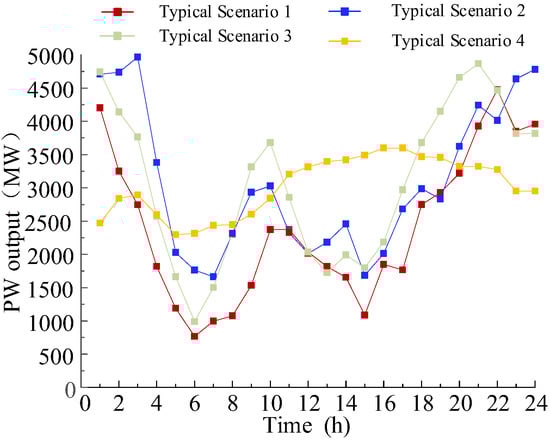
Figure 6.
Wind power output curve.
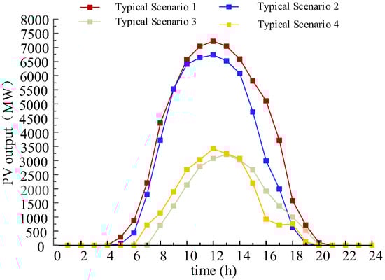
Figure 7.
PV output curve.

Table 1.
Comparison of the characteristics of electric energy storage and hydrogen energy storage.
5.1. Planning Configuration Results
5.1.1. Comparative Analysis of Configuration Results and Economic Performance
Four comparative schemes are established:
Scheme 1: Grid-forming ESS and HESS participate in frequency regulation with fixed parameters.
Scheme 2: Grid-forming EES alone provides frequency regulation with fixed parameters.
Scheme 3: HESS alone provides frequency regulation with fixed parameters.
Scheme 4: Grid-forming EES and HESS participate in frequency regulation with optimized parameters.
The configuration results under different schemes are summarized in Table 2.
Table 2.
System control parameters and economic parameters.
As shown in Table 3, compared with Scheme 1, the configuration results of the proposed Scheme 4 show reductions of 4.60%, 8.24%, 1.27%, 11.12%, and 4.16% in the rated power and capacity of the grid-forming electrochemical energy storage system, electrolyzer rated power, hydrogen storage tank capacity, and hydrogen fuel cell capacity, respectively. These reductions are primarily attributed to the optimization of virtual inertia time constants and primary frequency regulation coefficients, which enables more effective utilization of the inertia and frequency support capabilities of both EES and HESS.
Table 3.
Configuration results and costs of grid-forming EES and hydrogen energy storage.
As illustrated in Figure 13, Scheme 4 achieves superior performance across all three key frequency performance metrics. According to Equation (43), the improved RoCoF under Scheme 4 means that less EES capacity is needed to ensure frequency stability, thereby reducing the overall required storage configuration. Consequently, Scheme 4 successfully balances the need for frequency security with reductions in both EES and HES system capacity, resulting in enhanced economic performance.
Scheme 4 reduces the average daily investment cost by 22.33% compared to Scheme 2. This improvement arises from leveraging grid-forming EES and HES as sources of system inertia. Given the relatively lower cost of hydrogen storage, optimizing the virtual inertia time constants and primary frequency regulation coefficients allows Scheme 4 to meet frequency performance requirements while significantly reducing the total investment cost for the renewable energy base.
Relative to Scheme 3, the average daily investment cost under Scheme 4 decreases by 18.04%. This benefit stems from the strong inertia and frequency support capabilities of EES, which, when integrated with HES through coordinated grid-forming control, achieves a better balance between frequency metrics and economic efficiency. Figure 13 further confirms that Scheme 4 delivers superior frequency indicators across all three metrics, whereas Scheme 3 underperforms in all four representative scenarios. While HES alone can fulfill frequency regulation tasks, its relatively weaker response characteristics require greater configuration capacity, thus leading to inferior economic performance.
In summary, compared with other schemes, the proposed Scheme 4 effectively ensures frequency security through coordinated configuration of grid-forming EES and HES systems. By optimizing virtual inertia and frequency regulation parameters, Scheme 4 reduces excessive system configuration while improving overall economic efficiency.
5.1.2. Operation Mode of Electrochemical and HESS
To validate the effectiveness of grid-forming EES and HES systems in maintaining power balance under a weak AC system environment, the operational curves under four typical scenarios are presented in Figure 8. As observed, the DC export power fluctuates with variations in wind and solar output. A constraint mechanism on DC operation duration is introduced to ensure power stability: within the defined time window, the DC export power is maintained at a constant level.
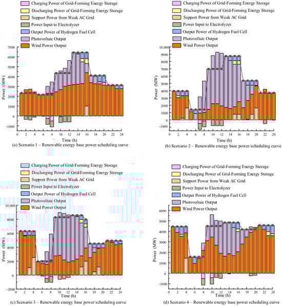
Figure 8.
Operation curve of the new energy base.
When wind and solar generation is high, the constraint prevents the DC export power from ramping up rapidly. The surplus energy is absorbed and stored by the EES and HES systems. Conversely, when renewable output declines and is insufficient to meet the export demand, the EES and HES systems promptly discharge to compensate for the power shortfall. This coordinated operational strategy ensures stability and continuity of DC power export.
Overall, the synergistic operation of grid-forming electrochemical and HESS plays an important role in enhancing the flexibility and reliability of large-scale renewable energy bases.
5.1.3. Inertia Support Capability of the Renewable Energy Base
The primary sources of system inertia in a renewable energy base include grid-forming wind farms and grid-forming EES and HESS. During nighttime, higher wind speeds typically enable wind farms to contribute substantial inertia. However, during daylight hours, due to weaker wind conditions, the inertia contribution from wind farms becomes insufficient, leading to a degradation in system frequency performance metrics. In such cases, additional inertia support is required from grid-forming EES and HES systems to facilitate rapid frequency recovery following disturbances.
As observed from Figure 9, the time period from 09:00 to 16:00 represents the interval of peak system inertia demand. During this period, the inertia provided by the PW is critically insufficient, posing a heightened risk of system instability. When grid-forming EES is incorporated, the system is able to meet the minimum requirements for the RoCoF in most scenarios. However, the achieved RoCoF performance only marginally satisfies the system’s alert threshold, indicating persistent operational risks.
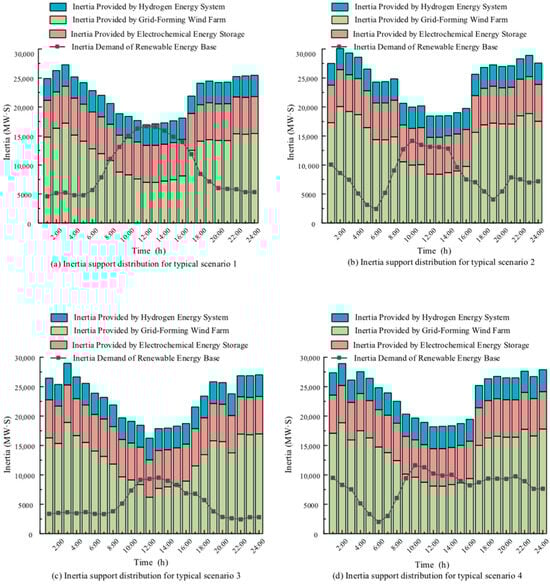
Figure 9.
Inertia support of the new energy base.
Upon integrating the hydrogen energy storage system, coordinated inertia response from both EES and HES significantly enhances the total system inertia during periods of low wind generation. This combined support ensures that the renewable energy base can withstand frequency disturbances more effectively, thereby improving the RoCoF performance metric and enhancing overall frequency stability.
5.2. Frequency Regulation Performance Analysis
5.2.1. Analysis of Frequency Regulation Parameter Optimization
Taking Typical Scenario 1 as an example, the comparison between Scheme 1, which uses fixed primary frequency regulation coefficients and virtual inertia time constants, and Scheme 4, which employs optimized parameters, is illustrated in Figure 10.
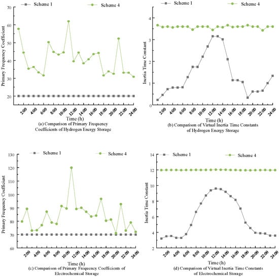
Figure 10.
Comparison of virtual inertia time constant and primary frequency modulation coefficient.
Figure 10 shows the optimized profiles of virtual inertia time constants and primary frequency regulation coefficients over 24 time intervals. The curves indicate that the system dynamically increases both parameters during critical periods—such as midday hours—when frequency fluctuations are more severe due to reduced wind inertia. This strategic adjustment strengthens the system’s response capability precisely when needed most. During periods of lower risk (e.g., early morning and late evening), the parameters are correspondingly reduced to avoid excessive regulation stress and energy consumption. This behavior illustrates the effectiveness of the bi-level optimization framework in achieving adaptive control. The improved frequency indicators associated with these dynamic adjustments are further confirmed in Figure 10, Figure 11 and Figure 12, where Scheme 4 consistently outperforms fixed-parameter schemes.
5.2.2. Frequency Performance Analysis
To further validate the effectiveness of the proposed grid-forming electrochemical and hydrogen energy storage systems in enhancing frequency stability, Typical Scenario 1 under Scheme 4 is analyzed in detail. The frequency rate-of-change curve and frequency deviation curve across 24 time intervals are shown in Figure 11 and Figure 12, respectively.
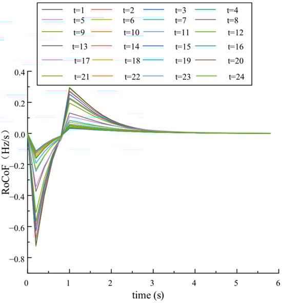
Figure 11.
Rate of frequency change curve.
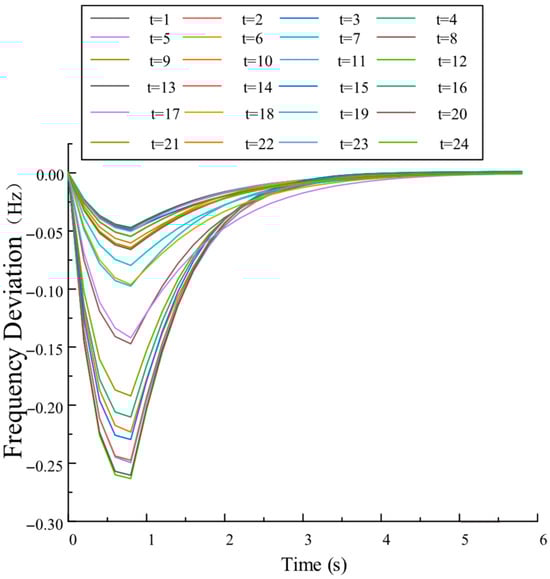
Figure 12.
Frequency deviation curve.
As shown in Figure 11, immediately after a disturbance occurs, the RoCoF rapidly decreases and reaches its minimum at the first time step. At the second time step, the RoCoF quickly rebounds to a positive value and then gradually approaches zero. Meanwhile, as illustrated in Figure 12, the frequency deviation continues to increase until the RoCoF becomes positive. Once the RoCoF turns positive, the frequency deviation begins to decline and gradually returns to its nominal value within the frequency regulation cycle.
This dynamic behavior occurs because a large-scale disturbance initially impacts the system’s RoCoF, causing it to plunge. As frequency deviation increases, the grid-forming wind farm, EES, and HESS rapidly activate to provide inertia support and frequency response. Throughout the regulation cycle, both RoCoF and frequency deviation decrease progressively, eventually stabilizing within acceptable limits.
By analyzing the RoCoF and frequency deviation curves over 24 time intervals under four typical scenarios, the frequency performance indicators are summarized in Figure 13.
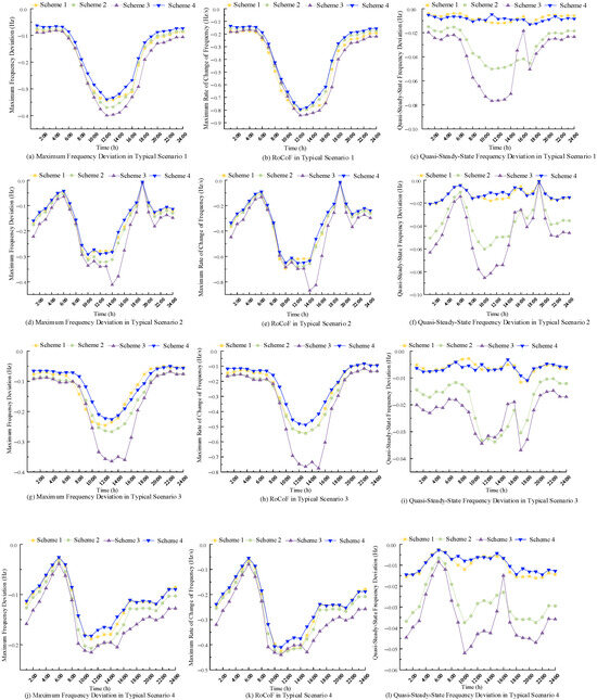
Figure 13.
Frequency index curve of the new energy base.
As shown in Figure 13, under Scheme 4, the detailed frequency indicators are as follows: In Scenario 1, the maximum frequency deviation and RoCoF occur at 12:00, with values of −0.3714 Hz and −0.8552 Hz/s, respectively, and the maximum quasi-steady-state frequency deviation appears at 16:00 with a value of −0.0142 Hz. In Scenario 2, the corresponding values at 12:00 are −0.2901 Hz and −0.6518 Hz/s, with the quasi-steady-state deviation at 08:00 being −0.0207 Hz. In Scenario 3, maximum deviation and RoCoF at 12:00 are −0.2118 Hz and −0.4881 Hz/s, while the quasi-steady-state deviation at 18:00 is −0.0109 Hz. In Scenario 4, the maximum deviation and RoCoF occur at 11:00 with values of −0.1823 Hz and −0.4098 Hz/s, and the quasi-steady-state deviation at 10:00 is −0.0145 Hz.
All frequency performance indicators in these four scenarios remain within the prescribed safety thresholds, indicating that Scheme 4 successfully meets the frequency stability requirements of the renewable energy base.
Compared with Scheme 1, the proposed parameter optimization method in Scheme 4 yields the following improvements across the four typical scenarios: maximum frequency deviation improved by 1.46%, 6.45%, 9.83%, and 3.48%; maximum RoCoF improved by 0.94%, 6.16%, 11.47%, and 3.62%; and maximum quasi-steady-state deviation improved by 0.70%, 11.99%, 3.60%, and 9.94%. These improvements are attributable to enhanced coordination between EES and HES systems achieved by optimizing primary frequency regulation coefficients and virtual inertia time constants. This optimization enables both systems to deliver their full frequency response potential while reducing their respective configuration costs.
Compared with Scheme 2, the proposed optimization method provides the following enhancements: maximum frequency deviation improved by 8.52%, 10.11%, 17.36%, and 12.05%; maximum RoCoF improved by 0.79%, 3.86%, 11.75%, and 5.66%; and maximum quasi-steady-state deviation improved by 74.32%, 65.64%, 77.82%, and 61.23%. Although HES has weaker frequency regulation capability, its low cost and inertia potential make it a valuable complement to EES when parameters are jointly optimized, significantly enhancing system performance.
Compared with Scheme 3, which utilizes only EES, Scheme 4 demonstrates even greater improvements: maximum frequency deviation improved by 15.49%, 14.68%, 40.14%, and 15.29%; maximum RoCoF improved by 5.91%, 6.52%, 36.16%, and 6.97%; and maximum quasi-steady-state deviation improved by 83.20%, 75.73%, 68.04%, and 72.06%. These gains indicate that integrating EES with HES under optimized frequency regulation parameters significantly reduces the risk of system instability, thanks to the stronger inertia and regulation capacity of EES.
In comparison to Schemes 1 through 3, the superior performance of Scheme 4 arises from its coordinated optimization of both system capacity and dynamic frequency response parameters. Unlike the heuristic or fixed-parameter approaches, Scheme 4 allows the virtual inertia constants and primary frequency regulation coefficients to be jointly tuned with the storage sizing process. This results in improved damping and frequency nadir control without requiring excessive oversizing of energy storage systems. Moreover, the model ensures that the frequency stability constraints are met dynamically under different operating scenarios, which enhances both cost-effectiveness and frequency resilience. Therefore, the advantage of Scheme 4 is not solely due to parameter optimization in isolation, but rather due to its systemic integration of planning and control objectives.
In conclusion, Scheme 4, by incorporating coordinated grid-forming control of electrochemical and hydrogen energy storage and by optimizing frequency regulation parameters, effectively enhances the frequency stability of large-scale renewable energy bases while minimizing associated costs.
6. Conclusions
- (1)
- The proposed bi-level optimization model effectively balances frequency security and economic efficiency. By dynamically adjusting primary frequency regulation parameters for both EES and HES under various operating scenarios, it optimizes system configuration and reduces investment costs while maintaining frequency stability.
- (2)
- Compared to schemes using fixed regulation parameters, the optimized configuration improves both frequency safety and system cost-effectiveness. Particularly, the collaborative use of grid-forming EES and HES under optimized control ensures reliable operation while lowering capital expenditures.
- (3)
- Compared with single-source schemes using only EES or HES, the hybrid configuration significantly enhances frequency indicators, reduces the risk of frequency excursions, and improves both frequency stability and economic performance.
Currently, most renewable energy base planning models primarily address frequency response, with limited research on voltage support. To fully leverage the potential of grid-forming ESS, future work should explore the joint optimization of voltage support and frequency response in renewable energy base planning.
Author Contributions
D.H.: review, editing, software, resources, methodology, data curation, and conceptualization. P.S.: writing—original draft, software, investigation, and formal analysis. W.Y.: supervision, project administration, and funding acquisition. C.L.: resources, formal analysis, and data curation. H.Z.: writing—review and editing. Y.G.: writing—review and editing. All authors have read and agreed to the published version of the manuscript.
Funding
This research was funded by the National Key Research and Development Program of China, grant number 2021YFB2400905; The Science and Technology Project of CSG Electric Power Research Institute Co., Ltd., grant number SEPRI-K223023.
Data Availability Statement
The original contributions presented in this study are included in the article. Further inquiries can be directed to the corresponding author.
Conflicts of Interest
Authors Dongqi Huang, Pengwei Sun, Wenfeng Yao, Hefeng Zhai and Yehao Gao were employed by the company CSG Electric Power Research Institute Co., Ltd. All authors declare that the research was conducted in the absence of any commercial or financial relationships that could be construed as potential conflicts of interest.
References
- Li, Z.; Xu, Y.; Wang, P.; Xiao, G. Restoration of Multi Energy Distribution Systems with Joint District Network Recon Figureuration by a Distributed Stochastic Programming Approach. IEEE Trans. Smart Grid 2023, 15, 2667–2680. [Google Scholar] [CrossRef]
- Saleem, M.I.; Saha, S.; Roy, T.K. A frequency stability assessment framework for renewable energy rich power grids. Sust. Energy Grids Netw. 2024, 38, 101380. [Google Scholar] [CrossRef]
- Qin, B.; Wang, M.; Zhang, G.; Zhang, Z. Impact of renewable energy penetration rate on power system frequency stability. Energy Rep. 2022, 8, 997–1003. [Google Scholar] [CrossRef]
- Xue, X.; Ai, X.; Fang, J.; Cui, S.; Jiang, Y.; Yao, W.; Chen, Z.; Wen, J. Real-time Schedule of Microgrid for Maximizing Battery Energy Storage Utilization. IEEE Trans. Sustain. Energy 2022, 13, 1356–1369. [Google Scholar] [CrossRef]
- Zhang, R.; Chen, Y.; Li, Z.; Jiang, T.; Li, X. Two-stage robust operation of electricity-gas-heat integrated multi-energy microgrids considerin g heterogeneous uncertainties. Appl. Energy 2024, 371, 123690. [Google Scholar] [CrossRef]
- Elsaied, M.M.; Abdel Hameed, W.H.; Hasanien, H.M. Frequency stabilization of a hybrid three-area power system equipped with energy storage units and renewable energy sources. IET Renew. Power Gen. 2022, 16, 3267–3286. [Google Scholar] [CrossRef]
- González-Inostroza, P.; Rahmann, C.; Álvarez, R.; Haas, J.; Nowak, W.; Rehtanz, C. The role of fast frequency response of energy storage systems and renewables for ensuring frequency stability in future low-inertia power systems. Sustainability 2021, 13, 5656. [Google Scholar] [CrossRef]
- Kerdphol, T.; Rahman, F.S.; Mitani, Y. Virtual inertia control application to enhance frequency stability of interconnected power systems with high renewable energy penetration. Energies 2018, 11, 981. [Google Scholar] [CrossRef]
- Shu, Y.; Tang, Y. Analysis and recommendations for the adaptableility of China’s power system security and stability relevant standards. CSEE J. Power Energy Syst. 2017, 3, 334–339. [Google Scholar] [CrossRef]
- Du, W.; Fu, Q.; Wang, H.F. Power System Small-Signal Angular Stability Affected by Virtual Synchronous Generators. IEEE Trans. Power Syst. 2019, 34, 3209–3219. [Google Scholar] [CrossRef]
- Wang, K.; Wang, C.; Yao, W.; Zhang, Z.; Liu, C.; Dong, X.; Yang, M.; Wang, Y. Embedding P2P transaction into demand response exchange: A cooperative demand response management framework for IES. Appl. Energy 2024, 367, 123319. [Google Scholar] [CrossRef]
- Liu, J.; Yang, D.; Yao, W.; Fang, R.; Zhao, H.; Wang, B. PV-Based Virtual Synchronous Generator with Variable Inertia to Enhance Power System Transient Stability Utilizing the Energy Storage System. Prot. Control Mod. Power Syst. 2017, 2, 1–8. [Google Scholar] [CrossRef]
- Aghdam, S.A.; Agamy, M. Virtual oscillator-based methods for grid-forming inverter control: A review. IET Renew. Power Gener. 2022, 16, 835–855. [Google Scholar] [CrossRef]
- Meng, X.; Liu, J.; Liu, Z. A generalized droop control for grid-supporting inverter based on comparison between traditional droop control and virtual synchronous generator control. IEEE Trans. Power Electron. 2018, 34, 5416–5438. [Google Scholar] [CrossRef]
- Shi, T.; Sun, J.; Han, X.; Tang, C. Research on adaptive optimal control strategy of virtual synchronous generator inertia and damping parameters. IET Power Electron. 2024, 17, 121–133. [Google Scholar] [CrossRef]
- Rathnayake, D.B. Control Design of Inverter-based Resources in Power Systems. Ph.D. Thesis, Monash University, Clayton, Australia, 2023. [Google Scholar]
- Dedeoglu, S.; Konstantopoulos, G.C.; Komurcugil, H. Current-Limiting Virtual Synchronous Control and Stability Analysis Considering DC-Link Dynamics Under Normal and Faulty Grid Conditions. IEEE J. Emerg. Sel. Top. Power Electron. 2022, 10, 2516–2527. [Google Scholar] [CrossRef]
- Magdy, G.; Shabib, G.; Elbaset, A.A.; Mitani, Y. Renewable power systems dynamic security using a new coordination of frequency control strategy based on virtual synchronous generator and digital frequency protection. Int. J. Electr. Power Energy Syst. 2019, 109, 351–368. [Google Scholar] [CrossRef]
- Li, D.; Zhu, Q.; Lin, S.; Bian, X.Y. A Self-Adaptive Inertia and Damping Combination Control of VSG to Support Frequency Stability. IEEE Trans. Energy Convers. 2017, 32, 397–398. [Google Scholar] [CrossRef]
- Zhang, X.; Mao, F.; Xu, H.; Liu, F.; Li, M. An optimal coordination control strategy of micro-grid inverter and energy storage based on variable virtual inertia and damping of vsg. Chin. J. Electr. Eng. 2017, 3, 25–33. [Google Scholar]
- Li, C.; Yang, Y.; Mijatovic, N.; Dragicevic, T. Frequency Stability Assessment of Grid-Forming VSG in Framework of MPME with Feedforward Decoupling Control Strategy. IEEE Trans. Ind. Electron. 2022, 69, 6903–6913. [Google Scholar] [CrossRef]
- Liu, C.; Chu, Z.; Duan, Z.; Zhang, Y. VSG-Based Adaptive Optimal Frequency Regulation for AC Microgrids With Nonlinear Dynamics. IEEE Trans. Autom. Sci. Eng. 2024, 22, 1471–1482. [Google Scholar] [CrossRef]
- Ge, L.; Zhang, B.; Huang, W.; Li, Y.; Hou, L.; Xiao, J.; Mao, Z.; Li, X. A review of hydrogen generation, storage, and applications in power system. J. Energy Storage 2024, 75, 109307. [Google Scholar] [CrossRef]
- Allahham, A.; Greenwood, D.; Patsios, C.; Walker, S.L.; Taylor, P. Primary frequency response from hydrogen-based bidirectional vector coupling storage: Modelling and demonstration using power-hardware-in-the-loop simulation. Front. Energy Res. 2023, 11, 1217070. [Google Scholar] [CrossRef]
- Jeong, Y.; Kim, G.; Lee, J.; Han, S. Hydrogen-Based Solutions for Enhancing Frequency Stability in Renewable Energy-Integrated Power Systems. Energies 2025, 18, 1562. [Google Scholar] [CrossRef]
- Li, J.; Hu, J.; Xin, D. Cooperative control of hydrogen-energy storage microgrid system based on disturbance-rejection model predictive control. J. Energy Storage 2025, 118, 116242. [Google Scholar] [CrossRef]
- Lee, G.-H.; Kim, Y.-J. Frequency Regulation of an Islanded Microgrid Using Hydrogen Energy Storage Systems: A Data-Driven Control Approach. Energies 2022, 15, 8887. [Google Scholar] [CrossRef]
- Xu, C.; Zhao, D.; Liu, H.; Bai, J.; Du, Z.; Tao, R.; Liu, C. An ESS planning approach for new energy bases without on-site conventional unit support. CSEE J. Power Energy Syst. 2025, 1–14. Available online: https://ieeexplore.ieee.org/stamp/stamp.jsp?arnumber=10838250 (accessed on 15 June 2025).
- Liu, Y.; Chen, Y.; Xin, H.; Tu, J.; Zhang, L.; Song, M. System Strength Constrained Grid-Forming Energy Storage Planning in Renewable Power Systems. IEEE Trans. Sustain. Energy 2025, 16, 981–994. [Google Scholar] [CrossRef]
Disclaimer/Publisher’s Note: The statements, opinions and data contained in all publications are solely those of the individual author(s) and contributor(s) and not of MDPI and/or the editor(s). MDPI and/or the editor(s) disclaim responsibility for any injury to people or property resulting from any ideas, methods, instructions or products referred to in the content. |
© 2025 by the authors. Licensee MDPI, Basel, Switzerland. This article is an open access article distributed under the terms and conditions of the Creative Commons Attribution (CC BY) license (https://creativecommons.org/licenses/by/4.0/).