Abstract
Accurate forecasting of electricity production is crucial for the stability of the entire energy sector. However, predicting future renewable energy production and its value is difficult due to the complex processes that affect production using renewable energy sources. In this article, we examine the performance of basic deep learning models for electricity forecasting. We designed deep learning models, including recursive neural networks (RNNs), which are mainly based on long short-term memory (LSTM) networks; gated recurrent units (GRUs), convolutional neural networks (CNNs), temporal fusion transforms (TFTs), and combined architectures. In order to achieve this goal, we have created our benchmarks and used tools that automatically select network architectures and parameters. Data were obtained as part of the NCBR grant (the National Center for Research and Development, Poland). These data contain daily records of all the recorded parameters from individual solar and wind farms over the past three years. The experimental results indicate that the LSTM models significantly outperformed the other models in terms of forecasting. In this paper, multilayer deep neural network (DNN) architectures are described, and the results are provided for all the methods. This publication is based on the results obtained within the framework of the research and development project “POIR.01.01.01-00-0506/21”, realized in the years 2022–2023. The project was co-financed by the European Union under the Smart Growth Operational Programme 2014–2020.
1. Introduction
The continuity and quality of the energy supplied by providers is a very important aspect of the correct, stable, and safe operation of any electrical installation. To ensure appropriate parameters for each end user, energy companies use forecasting methods to predict future demand. However, a significant challenge is the use of an energy mix in energy production using traditional power plants (e.g., coal, gas, and nuclear) and renewable sources such as photovoltaic or wind farms, for which production depends on the current weather conditions (insolation [1] and wind parameters [2], etc.). Traditional power plants have historically contributed significantly to grid stability by providing dispatchable base-load and flexible generation capacity. However, their inflexibility and environmental costs have led to a transition to more sustainable solutions.
On the other hand, renewable sources provide energy without causing greenhouse gas emissions. However, their output is inherently intermittent and variable. It is highly dependent on meteorological conditions, such as insolation, wind speed, temperature, and cloud cover. During extreme events such as prolonged cloud cover or windless conditions, their energy contribution can be minimal. To be able to launch the appropriate level of electricity production in traditional power plants, power grid operators need effective models for predicting renewable energy production well in advance. Combining this data with predictions of power consumption by grid users enables operators to launch the appropriate level of electricity production in traditional power plants. Accurate forecasting is also crucial beyond adjusting traditional power plant output. It is essential for optimizing the deployment of energy storage solutions, enabling efficient demand-side management, and facilitating grid-scale balancing initiatives that enhance overall system reliability and flexibility.
Creating such models is an essential step in planning and determining the operating parameters of electronic power systems. Many private companies and government institutes are involved in R&D programs to develop new algorithms and methods for forecasting renewable energy production.
Deep learning methods have emerged as a powerful alternative. Wen et al. applied deep neural networks (DNNs) to short-term load forecasting and achieved moderate gains over statistical models [3]. Shi et al. adapted Convolutional Neural Networks (CNNs) to extract spatial and temporal features from power grid data [4], and long short-term memory (LSTM) networks have consistently outperformed both feedforward and traditional recurrent architectures in sequential prediction tasks [5,6]. Gated recurrent units (GRUs) offer a computationally more efficient alternative to LSTMs with comparable accuracy [7]. Despite these advances, most studies have focused on forecasting a single variable, either electricity demand [8] or a specific type of renewable generation such as solar or wind [9,10]. These studies often use synthetic or publicly available datasets rather than region-specific, real-world measurements.
A few recent studies have investigated multi-target forecasting. For instance, separate LSTM models have been trained for load and solar generation, but their outputs have not been integrated or optimized for interaction. Additionally, previous studies rarely applied distinct modeling pipelines for different renewable sources despite the unique temporal dynamics and environmental dependencies of solar and wind systems. There has been limited research that unifies electricity demand, solar photovoltaic (PV), and wind power forecasting within a single deep learning framework, especially when using detailed meteorological and equipment-related features from operational data.
In this article, we analyze and propose different methods for forecasting renewable energy production. Next, we will test these methods against real data from wind and photovoltaic farms analyzed in our project, which is being implemented as part of an R&D grant established by the NCBR (the National Center for Research and Development, Poland).
In addition to exploring different methods of predicting renewable energy, an important innovative aspect of our work is automating the preparation of input data for various algorithms.
Accurately forecasting electricity demand is a critical task in the realm of energy sector stability, particularly amidst the intricate dynamics posed by renewable energy utilization. This study examines the effectiveness of deep learning models for electricity demand forecasting, providing an in-depth analysis of recursive neural networks (RNNs), including LSTM networks, gated recurrent units (GRUs), convolutional neural networks (CNNs), temporal fusion transformers (TFTs), and hybrid architectures.
This research innovatively integrates benchmark creation and uses automated tools for network architecture and parameter selection to facilitate robust model evaluation. The three-year dataset, sourced from the NCBR grant, includes daily readings from individual solar and wind farms.
The experimental findings particularly highlight the superiority of LSTM models in forecast accuracy, as they outperform their counterparts. The study also clarifies multilayer deep neural network (DNN) architectures and offers thorough results across different methodologies. This advances the discussion about efficiently predicting electricity demand in renewable energy landscapes.
2. Materials and Methods
As previously noted, the main goal of this paper is to present the research on recursive neural network (RNN) and deep neural network (DNN) models, that can solve complex tasks such as renewable energy production. Below, we briefly describe popular architectures that could be used for this purpose. To choose the best deep neural network (DNN) model, we used our benchmarks and automated method for selecting network architecture and parameters. We adopted the TSPP (Time-Series Prediction Platform) framework by NVIDIA to solve a specific forecasting problem for renewable energy sources.
Recurrent neural networks are deep learning models that are typically used to solve problems with sequential data (such as time series) [11]. The architecture of these networks has connections between individual cells that enable the network to emphasize and preserve previously occurring information to predict subsequent values. This is possible due to loops in the architecture, which reuse the output from one step as input data for the next step.
2.1. TSPP
The main advantage of using an automated environment to select multiple models is that comparing each result is easy. Each metric can be measured for each method at each stage of learning. Benchmarks can demonstrate the strengths and weaknesses of any architecture. One can also focus primarily on optimization aspects. This is also very helpful when evaluating multiple horizons and methods.
The Time-Series Prediction Platform is a popular framework for training, tuning, and deploying time-series models. Its hierarchical configuration system and rich feature specification API allow new models, datasets, optimizers, and metrics to be easily integrated and experimented with. The TSPP is designed for vanilla PyTorch models and is agnostic to the cloud or local platforms [12].
The proposed architecture presented in Figure 1 provides a platform for automatically selecting DNN algorithms for renewable energy applications. Processing a particular method or architecture requires several steps:
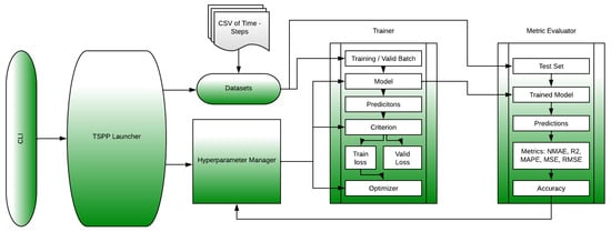
Figure 1.
The basic architecture of the NVIDIA Time-Series Prediction Platform (TSPP). The command-line interface (CLI) feeds the input to the TSPP launcher, which instantiates the objects required for training such as the model and dataset. The launcher then runs the specified experiment to generate performance and accuracy results [12].
- Loading data from a CSV file after processing;
- Data preparation (dividing the data into training and test sets);
- Running the training script (building the model and training the selected DNN);
- Creation of a validation script (evaluating using the appropriate metrics and creating a report based on the results). Optionally, the appropriate hyperparameters are modified.
NVIDIA TSPP is an automated tool that makes it easy to compare and experiment with any combination of time-series datasets, predictive models, and their configurations and hyperparameters. The TSPP provides the ability to identify optimal hyperparameter search spaces, and to run accelerated model training using distributed multi-GPU training with automatically selected precision [12].
2.2. Statistical Methods
2.2.1. Naive Method—As a Benchmark, a Reference Point
Naive forecasting is the simplest method of estimating future values. In this method, the value from the previous period (denoted by ) is assigned as the forecast value for the next period. This method works exceptionally well for many economic and financial time series. For longer prediction horizons, we use the last known value, i.e., the value at time t-h. We write it as follows:
where
- : forecast of the explanatory variable determined for period t;
- : the value of the forecasted variable in the previous period (i.e., the period ).
2.2.2. LASSO
The LASSO method is a generalization of linear regression. It involves adding the so-called regularization to the algorithm that calculates the value of the parameter . In this case, we are dealing here with the L1 norm, which causes many vector values of the model parameters —which are small but non-zero in linear regression— to become exactly zero. This behavior is useful when there are a large number of explanatory variables. This approach selects the features with the strongest linear relationship to the explanatory variable. The LASSO method has one hyperparameter, usually denoted by , which determines the strength of regularization. The higher the value of this parameter, the more vector elements will be equal to zero, and the fewer features will be selected for the model. When provides the linear regression described in the previous point is obtained. Introducing regularization into the model usually yields models that perform better with new data. This is because the model retains only the strong relationships evident in the training set. Several apparent dependencies are eliminated because of this. However, too much regularization prevents the models from learning important dependencies. Therefore, the value of should be selected by dividing the data into learning, validation, and test sets. The LASSO method can also be used to preselect variables for training other models. For this purpose, a small value is usually used (), which discards variables with little or no relationship to the explanatory variable.
2.3. ML Methods
2.3.1. RF Random Forest
This method is based on the idea that an average of many average-quality models works better than each model individually. The idea is that the random errors of the models will average out, making the final prediction more accurate. For this method to work, it is important that the models whose results are used to calculate the mean differ significantly from each other. In the case of a random forest, simple decision trees are used as medium-quality models.
The depth of a single tree is typically the most important hyperparameter of the model. Another important hyperparameter is the number of trees in the forest. Random factors ensure differences between individual trees. First, each tree is trained using a different set of data. This set is generated as a bootstrap sample from the entire learning set. The second mechanism involves randomly selecting a subset of learning traits. Due to this, each tree is based on different variables, ensuring that the same features do not repeat constantly. This method is one of the most effective in all kinds of machine learning competitions.
2.3.2. XGBoost
Like a forest, the gradient boosting method is a random method that uses many random trees. A random forest is an ensemble bagging method in which many different models are analyzed simultaneously (informally ”thrown into one bag”) and the average of their predictions is calculated. Boosting, on the other hand, sequentially creates subsequent trees. Each subsequent tree is designed to best predict the residuals remaining after the previous trees have made their predictions (in other words, after each run, we try to match the new predictor to the residual error made by the previous predictor). Subsequent models improve the results of previous ones in this way. Methods of this type are widely used in practice. The present study employed an implementation from the XGBoost library, which is regarded as one of the most expeditious and precise solutions currently available. The hyperparameters that were searched included the maximum number of leaves in the tree, the number of trees reinforced with a gradient, and the parameter responsible for regularization, the learning speed.
2.4. DNN Methods
2.4.1. LSTM
As part of the work, the LSTM network layers were used. These layers operate based on two state vectors: short-term h and long-term c. The network also uses forget gates. This design enables the cell to determine which inputs are important and how long to retain them in the long-term memory vector. The previous state of the cell is then saved in short-term memory. The forget gate determines the lifespan of the information contained in the long-term vector. Information kept in long-term memory is removed when it ceases to be relevant Figure 2. This is ideal for sectors related to text, speech, or audio recording analysis, as well as time-series analysis.
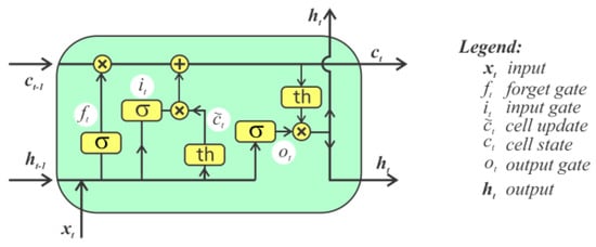
Figure 2.
LSTM architecture [13].
2.4.2. GRU
The GRU (gated recurrent unit) cell is a simplified version of the LSTM. In the GRU, both state vectors are combined into a single h(t) vector. One gate controller manages both the forget and entrance gates. When the gate controller displays 11, the entrance gate is open and the forget gate is closed. In contrast, when the result is 00, the opposite is true Figure 3. In other words, when memory needs to be stored, the place where it will be written is first cleared.
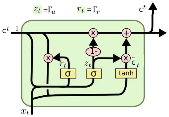
Figure 3.
GRU architecture [14].
2.4.3. CNN
Both CNN and LSTM/GRU networks consist of layers of convolutional and recursive networks. The CNN layer is designed to reduce the problem space. Convolutional networks are designed to draw dependencies between two functions. For example, with the help of a convolutional network, we can draw dependencies between functions f and g, which allows recursive networks to learn individual dependencies better. This structure is effective for analyzing sound and speech because it processes large amounts of data based on when they occur relative to each other. Typically, the layers of convolutional networks occur at the beginning of the model, and their output is fed to the LSTM/GRU layer. One disadvantage of this solution is that convolutional networks usually require a large amount of data to learn.
Convolutional neural networks (CNNs) are a type of artificial neural network that learns through mathematical convolution operations. Like traditional neural networks, CNNs consist of layers: an input layer, hidden layers, and an output layer. The main difference is that, in addition to the activation function, the hidden layers of CNNs use the convolution of the layer and filter input data. CNNs are widely used in image processing and analysis. One-dimensional convolutional networks (1D CNNs) use two-dimensional data as input Figure 4. They are used in time-series analysis, among other applications.
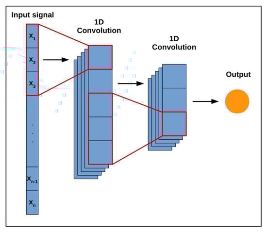
Figure 4.
One-dimensional CNN architecture [15].
2.4.4. TFT
The Temporal Fusion Transformer (TFT) is an advanced model that allows for the interpretation and multi-horizon prediction of time series data. Google first developed and implemented the model in collaboration with the University of Oxford. It is a hybrid architecture combining LSTM encoding of time series with the interpretability of Transformer attention layers. Predictions are based on three types of variables: static (constants for a given time series), known (known in advance for the entire time series), and observed (known only from historical data) Figure 5. These variables come in two varieties: categorical and continuous. In addition to historical data, we feed the model historical values of the time series. All variables are embedded in a multidimensional space using the embedding vector. Categorical variables are embedded in the classical sense of embedding discrete values. The model learns a single vector for each continuous variable and scales it by the variable’s value for further processing [16].
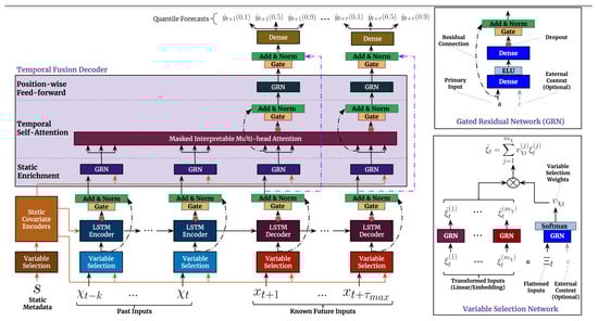
Figure 5.
NVIDIA temporal fusion transformer model architecture [16].
2.5. Data Preprocessing
To ensure data quality, consistency, and optimal model performance, the raw datasets underwent several preprocessing steps. These steps included:
- Handling missing values: Missing data points were carefully selected to preserve data integrity and temporal relationships.
- Outlier treatment: Outliers were identified and managed through transformation to mitigate their undue influence on model training.
- Data normalization/scaling: All numerical features were Min–Max-scaled to a range of [0, 1] range or standardized to a mean of 0 and a standard deviation of 1. Scaling parameters were derived solely from the training set and applied consistently across all datasets to prevent data leakage and facilitate model convergence.
2.6. Data Preparation EDA
After preparing and supplementing the data, an exploratory analysis was conducted on all data received from the energy sub-supplier. Based on this analysis, data was selected to train the tested models. The following areas were selected from all received files:
Data on energy production from renewable sources:
Data on photovoltaic panel energy production. This data came from six farms. Approximate location of farms are shown on Figure 6 The data were sampled at 15-minute intervals. Depending on the variant, weather and event data (SCADA) were added to the data from each farm (merged measurements from the inverters). Additionally, energy generation forecasts based on weather forecasts and energy meter data delivered to the grid were provided.
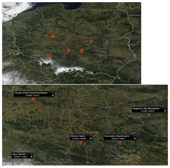
Figure 6.
Approximate locations of photovoltaic farms in Poland whose data were used in the project.
The coordinates of the photovoltaic farms are listed below.
- Żerków, Wielkopolskie, Poland: 52.0367°, 17.6395°.
- Żerków, Wielkopolskie, Poland: 52.0409°, 17.6714°.
- Nysa, Opolskie, Poland: 50.4481°, 17.3637°.
- Kłobuck, Śląskie, Poland: 50.9193°, 18.8936°.
- Kluczewsko, Świętokrzyskie, Poland: 50.9187°, 19.9091°.
- Mogielnica, Mazowieckie, Poland: 51.6342°, 20.6678°.
In order to build predictive models, only a dozen or so features common to each solar farm were taken into account:
- date (timestamp) in UNIX format;
- total value from the sun sensor;
- daily value from the insolation sensor;
- PV module temperature (average);
- outdoor temperature;
- weather (solar radiation and cloudiness);
- input voltage (common to each of the inverters);
- temperature inside the inverter (average value);
- input voltage from the power grid;
- current;
- frequency;
- power factor;
- active power;
- input power;
- energy throughout its lifetime;
- inverter efficiency;
- power produced by the inverter (average);
- daily value of energy produced.
Data on wind energy production. The data came from four farms. Samples were taken every 10 min. Data on weather forecasts, sampled every hour, and a forecast of electricity generation based on the weather forecasts were also available for the four farms. The projected amount was electricity production. After breaking down the data, four series were submitted for analysis.
In order to build predictive models, only about a dozen features common to each wind farm should be considered:
- average generator RPM;
- generator bearing temperature;
- gearbox bearing temperature;
- gondola temperature;
- rotor RPM;
- wind speed;
- wind direction;
- ambient temperature;
- power delivered to the grid;
- L1 voltage;
- L2 voltage;
- L3 voltage;
- L1 current;
- L2 intensity;
- L3 intensity;
- the direction of the gondola;
- turret acceleration;
- gear temperature;
- the average angle of inclination of the blades.
2.7. Used Metrics
- is a statistical measure that represents the proportion of the variance in the dependent variable explained by more than one independent variable in a regression model. The R-squared value is the opposite of the correlation and shows how much one variable’s variance explains another variable’s variance. Correlation explains the strength of the relationship between the independent and dependent variables. Therefore, if the R2 of one is equal to 0.50, then model inputs can explain half of the observed variability.
- Normalized mean absolute error (NMAE), also known as the MAE coefficient of variation, is another useful metric. This metric is mainly used to compare MAEs of datasets with different scales. Normalization means that the model performance evaluation tool uses the average of the measured data.
- The root mean squared error (RMSE) is calculated as the standard deviation of the residuals (prediction errors). Prediction errors are measured as the distance from the regression line to the data points. RMSE measures how dispersed these prediction errors/residuals are. It indicates how concentrated the data are around the line of best fit. The mean squared error is widely used in forecasting, climatology, and regression analysis to validate experimental results.
- Mean absolute error (MAE) is a metric used to quantify the average magnitude of the difference between predicted and actual values in a dataset. Unlike other error metrics, MAE calculates the absolute difference between the two values, regardless of the direction of the error. Consequently, MAE provides a straightforward, interpretable measure of model performance by representing the average deviation of predictions from ground-truth values.
- The mean pinball loss (MPL) is a metric commonly used in quantile regression and forecasting tasks. It is sometimes referred to as quantile loss. It measures the deviation between predicted quantiles and actual observations. For a given set of quantiles (e.g., 0.1, 0.5, 0.9), the mean pinball loss is the average pinball loss across all quantiles.
- The median absolute error (MEAE) is a metric used in regression tasks to quantify the median magnitude of the difference between predicted and actual values. Similar to the mean absolute error (MAE), it calculates the median absolute difference instead of averaging the absolute differences between predictions and actuals.
- The explained variance score (EVS) is a metric used to evaluate the performance of regression models. It quantifies the proportion of variance in the target variable that is explained by the model. EVS scores range from −∞ to 1. A score of 1 indicates a perfect prediction, meaning the model explains all the variance in the target variable. A score of 0 indicates that the model’s predictions are no better than simply predicting the mean of the target variable. Negative scores can occur if the model performs worse than the mean prediction. In summary, the explained variance score provides insight into how well the model captures the variance in the target variable.
This manuscript presents the experimental results obtained from evaluating various forecasting models, including multilayer deep neural network (DNN) architectures [17]. Our analysis encompasses the performance of all the methods we investigated. To thoroughly examine the problem of energy forecasting, the models were tested on real-world energy production data from individual photovoltaic and wind farms, as well as on their total energy output [18]. This allows us to gain detailed understanding of how the models behave across different scenarios.
This publication draws upon findings from the research and development project POIR.01.01.01-00-0506/21”, carried out during 2022–2023. The project received co-financing from the European Union as part of the Smart Growth Operational Programme 2014–2020.
2.8. Chosen Hyperparameters
2.8.1. Multi-LSTM Model Hyperparameters
Our innovative framework features a hybrid DNN-LSTM model that seamlessly combines the robust capabilities of DNNs with the nuanced sequence modeling prowess of LSTM networks. This combination provides a powerful solution for navigating the complex landscape of sequential data challenges. At the core of the model is an LSTM layer with 200 units, which serves as the foundation for temporal understanding. Each LSTM unit is imbued with the rectified linear unit (ReLU) activation function, which introduces essential nonlinear transformations that capture the subtle temporal dynamics encoded within the data.
On top of the LSTM foundation, a fully connected dense layer with 100 units is strategically positioned. Leveraging the ReLU activation function, this layer attempts to extract higher-level features and intricate patterns from the LSTM’s output. This adds a crucial layer of nonlinearity and abstraction to the model’s representation. The output layer, the final stage of the model architecture, is the nexus for crafting final predictions. While the activation function for this layer is not specified, assuming linear activation is reasonable. This layer synthesizes the model’s learning into actionable forecasts, serving as the harbinger of predictive insights. Through this meticulously crafted architecture, our hybrid DNN–LSTM model emerges as a beacon of innovation, adept at navigating the complexities of sequential data while harnessing the strengths of both DNNs and LSTMs.
2.8.2. Encoder–Decoder–Multi-LSTM Hyperparameters
Our fusion model, which combines DNNs and LSTMs, synergistically addresses the complexities of sequential data analysis. Our approach combines the feature extraction capabilities of DNNs with the temporal memory capabilities of LSTMs, ushering in a new era of predictive modeling [19].
At the core of the model is an LSTM layer with 200 units that serves as the foundational encoder. With the ReLU activation function, this layer provides the model with essential nonlinear transformations that capture the nuanced temporal patterns inherent in the input sequences.
Following the encoder is a RepeatVector layer that amplifies the encoded representation, preparing it for the subsequent LSTM decoder. Mirroring the encoder’s architecture with 200 units, the decoder orchestrates the generation of output across temporal steps with the help of TimeDistributed layers. The first TimeDistributed layer, with 100 units and ReLU activation, carefully dissects temporal intricacies. The subsequent TimeDistributed layer, with a single unit and linear activation, produces the final output.
The model compilation is founded on the strategic convergence of architectural components. The MSE loss function, adept at regression objectives, guides the optimization process alongside the Adam optimizer, which is renowned for its adaptive nature and rapid convergence.
In summary, our hybrid architecture, which is meticulously calibrated with LSTM-based encoders and decoders, provides a sophisticated framework for assimilating and generating sequences. Driven by meticulous loss minimization, this paradigm emerges as a beacon for tasks requiring intricate temporal dependencies and sequence-to-sequence forecasting.
3. Results
This section provides a thorough analysis of the performance of the predictive models applied to photovoltaic (PV) and wind energy datasets. Several key regression metrics were used to evaluate the models, including MAE, RMSE, NMAE, R2, and MAPE. The tested models include traditional regressors (e.g., Lasso, Random Forest, and XGBoost), standard deep learning architectures like LSTM, GRU, and CNN, and enhanced hybrid architectures (e.g., CNN-LSTM and Encoder-Decoder variants). Our results demonstrate the predictive power and robustness of deep learning methods for time-series energy forecasting [20].
3.1. Results of PV
Table 1 summarizes the model performance for PV farms. Among the classical models, XGBoost and RF demonstrated competitive performance, achieving NMAE values as low as 0.004 and R2 values of 0.91. The deep learning models, particularly the multi-step LSTM and conv–encoder–decoder–LSTM, yielded even better results with R2 exceeding 0.96 and RMSE below 11 kWh. These outcomes suggest that neural models have a superior capacity to capture the temporal dependencies and nonlinearities inherent in solar energy data.

Table 1.
Results for each method for PV farms.
Observation: The multi-step LSTM model outperformed the others due to its ability to maintain temporal memory across prediction windows. CNN-based methods also showed improvement, particularly when fused with LSTM encoders. This indicates that spatial-temporal correlations are essential for solar energy prediction.
3.2. Results of Wind
This section details our metrics and findings, showcasing the significant improvements in the accuracy of predicting energy output achieved by deep neural network (DNN) models for wind farms. Table 2 illustrates the prediction accuracy of various models applied to wind energy data. Performance variation across models is more pronounced in wind forecasting than in photovoltaics (PV), likely due to the higher volatility in wind generation.
Table 2.
Results for each method for wind farms.
Observation: Deep learning models, such as GRU and CNN, encountered challenges in certain evaluation scenarios, particularly in the EW2 setting. In contrast, multi-step LSTM and encoder-decoder LSTM models demonstrated consistent accuracy across various test cases, exhibiting significantly lower RMSE values compared to the baseline models.
3.3. Comparison with the Energy Received from the Weather Provider
A new test was conducted for more detailed analysis. We selected a day with significant cloud coverage variation for one of the solar farms. The graph below compares the energy produced with the readings provided by the weather provider and a working multi-LSTM model. To validate the practical applicability of our model, we made a day-specific comparison of the multi-LSTM predictions, weather forecasts, and actual energy production [21,22]. The results are presented in Table 3.
Table 3.
Solar farm energy/day comparison results.
The sudden increase in energy yield at 10 a.m. in the realization and multi-LSTM prediction columns, compared to the expected pattern observed in the forecast column, could be attributed to variations in solar activity.
A rapid intensification of sunlight or a decrease in cloud cover at 10 a.m. could have led to a sudden surge in solar energy production. This could result in a higher-than-expected energy yield at that time. The multi-LSTM prediction likely takes historical data and real-time conditions into account and may have accurately predicted this spike in energy production based on sun activity patterns.
In contrast, the gradual increase observed in the forecast column from 7:00 a.m. to 1:00 p.m., followed by a decrease, aligns with the typical diurnal pattern of solar energy production. As the sun rises and reaches its peak intensity around noon, solar energy production gradually increases. However, factors such as cloud cover or atmospheric conditions could influence the rate of increase and the overall peak energy yield. After reaching its maximum, solar energy production begins to decline as the sun’s angle decreases and the day progresses, resulting in the observed decrease in energy yield until 7 p.m Figure 7.

Figure 7.
Comparison of the predictions with the weather forecast and production data for selected PV farms.
Therefore, the discrepancy between the sudden increase in the realization and multi-LSTM prediction columns at 10 a.m. and the expected weather conditions suggests that localized variations in solar activity or unexpected atmospheric conditions might have played a role in altering the energy yield dynamics at that time.
3.4. Algorithmic Insights
While many of the models used in this study fall under known categories, such as LSTM and GRU, we adapted them with domain-specific enhancements:
- Multi-horizon and multi-step forecasting setups;
- Encoder–decoder–LSTM pipelines with convolutional preprocessing;
- Custom loss weighting to handle noisy intervals in wind data.
These enhancements render the framework semi-novel in context. Future work may involve exploring transformer-based architectures or hybrid ensemble models tailored to low-frequency meteorological data integration.
Novel Proposal (Suggested Future Work): We propose an ensemble learning system that integrates predictions from deep LSTM models and XGBoost residuals. These predictions are dynamically weighted based on local volatility estimation. This hybrid setup could improve generalization and robustness across varying weather conditions.
4. Discussion
Our experimental results confirm the effectiveness of data-driven models, particularly deep learning architectures, in forecasting renewable energy [23]. This section analyzes model performance, compares our findings with existing literature, outlines practical implications, and addresses study limitations.
For predicting electricity production from renewable energy sources, we tested an approach using DNN [24]. To this end, the data were properly prepared and accepted by the selected algorithms [25]. The data were transformed so that the indexes now refer to the correct dates. The interval between successive indexes is 15 or 10 min, depending on the dataset. The dependent variables are listed in the exploratory data analysis section.
It is worth emphasizing that the more data we provide to the model, the better the output results will be after applying the appropriate feature selection [26]. We have measured the accuracy of the models mainly using the R2 and NMAE (normalized mean absolute error) metrics.
To ensure a robust evaluation of the model’s performance and to prevent data leakage inherent in time-series forecasting, the dataset is split chronologically. The first 80 percent of the time-ordered data is designated as the training set and is used for model fitting. The remaining 20 percent is reserved as the test set for the final, unbiased evaluation of the trained models on unseen, future data. This sequential splitting strategy guarantees that all models are evaluated using data that follows their training period chronologically, thus simulating real-world forecasting scenarios. No data from the test set is used during training or hyperparameter tuning.
The results clearly demonstrate the superiority of data-driven models over classical methods in energy production forecasting. A key takeaway is that time-series-aware models with deep memory (e.g., multi-step LSTMs) significantly outperform static regressors. All visulisations are presented in Appendix A.
LSTM models perform better than other methods due to their superior ability to capture long-term temporal dependencies in time-series data and model complex nonlinear feature interactions, which are vital for volatile energy production patterns. Their capacity to benefit from extensive data volume during optimization contributes to their robust performance.
Additionally, extensive hyperparameter tuning and GPU-based training pipelines (via the NVIDIA TSPP and AGH Prometheus HPC systems) enable deeper optimization and reduced model variance. Traditional models quickly plateau during validation, whereas deep models continue to improve with epoch scaling and benefit from richer feature interactions.
This research yields accurate forecasts with significant practical implications. These include enhanced grid stability [27] through optimized dispatch of conventional power plants, improved electricity market operations, and reduced costs for system operators. These forecasts also facilitate the integration of renewable energy sources and provide a transferable methodology for broader application.
Key limitations include the study’s reliance on a specific geographic dataset [28], which may limit its generalizability, and the scope of the current input features. We observed slight overfitting of the GRU models in volatile datasets, which indicates the need for future work on more robust regularization and the inclusion of advanced features. Future research will also explore real-time operational integration and model interpretability.
One limitation that was observed is the slight overfitting of the GRU models in volatile wind datasets. This issue will be addressed in the future through the use of dropout regularization and attention-based mechanisms.
In summary, the results and discussion confirm that
- Deep models substantially improve the performance of both PV and wind farms.
- Forecasting accuracy varies depending on the model and energy source.
- Visual validation and real-day analysis underscore practical usability.
- The proposed hybridization (e.g., LSTM + XGBoost residuals) offers a direction for future research.
5. Conclusions
It is difficult to manually select the best model based only on metrics and graphical results. Thus, we used an automatic approach. Using our benchmarks and the NVIDIA TSPP framework, we have achieved the selection of proper hyperparameters and an optimized model in three dimensions (including calculation costs, weight, and performance).
The main advantage of using an automated environment to select multiple models is the ease with which each result can be compared. Each metric can be measured for each method at each stage of learning. The benchmarks demonstrate the advantages and disadvantages of each architecture. We can also focus primarily on optimization aspects. Additionally, it was helpful when evaluating multiple horizons and methods. For instance, in this project, there were three main horizons for each photovoltaic (PV) and wind farm, multiplied by different approaches, techniques, and architectures. Evaluating all the described methods took at least one and a half months.
To study the energy forecasting problem in detail, we tested the models’ behavior in the case of energy production from individual photovoltaic and wind farms based on the total energy production of the farms as a whole.
From a practical point of view, the main implementation goal (apart from the research topic of architectures, their applications, and methodologies) is to create the most reliable model for energy prediction for each farm. This aligns with the possibility of taking advantage of the developments in this scientific area. The choice of the LSTM network is random as well. This “lightweight” architecture makes it possible to use such models for embedded systems (e.g., STM32 microcontrollers protection).
In our study, we used a combination of AGH Prometheus, a high-performance computing cluster, and local department machines to meet the computational demands effectively. AGH Prometheus, which is known for its robust processing capabilities, was used for intensive tasks, such as training deep learning models and conducting large-scale simulations. The local department machines provided convenient resources for less demanding computations, ensuring an efficient allocation of resources throughout the research process. This strategic use of computational infrastructure allowed researchers to efficiently execute their experiments and advance their investigation of electricity demand forecasting with deep learning models.
While the proposed framework offers a comprehensive and scalable solution for model selection in energy forecasting, certain limitations require further examination. Notably, the evaluation process was limited by the lack of real-time production data and the assumption of consistent environmental conditions. Future research will focus on incorporating uncertainty quantification and exploring online learning strategies for dynamic model adaptation. Additionally, deploying and validating lightweight models on real-world embedded systems is a critical step toward practical implementation.
Author Contributions
Conceptualization, M.P. and A.K.; methodology, M.P. and A.K.; software, M.P.; validation, M.P., J.W. and A.K.; formal analysis, J.W.; investigation, M.P. and A.K.; resources, A.K.; data curation, A.K.; writing—original draft preparation, M.P.; writing—review and editing, M.P. and J.W.; visualization, M.P. and A.K.; supervision, J.W.; project administration, A.K. All authors have read and agreed to the published version of the manuscript.
Funding
This research received no external funding.
Data Availability Statement
The original contributions presented in this study are included in the article. Further inquiries can be directed to the corresponding author.
Conflicts of Interest
Appendix A. Proposed Architectures
Appendix A.1. PV
This subchapter presents visualizations of proposed hybrid architectures of PV farms for a time horizon of 1 h.
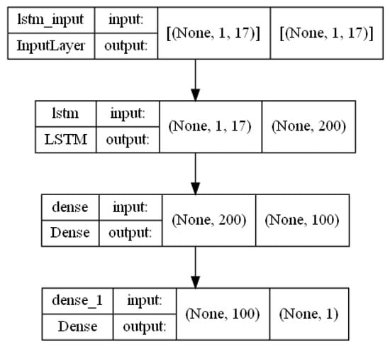
Figure A1.
Multi-LSTM architecture.
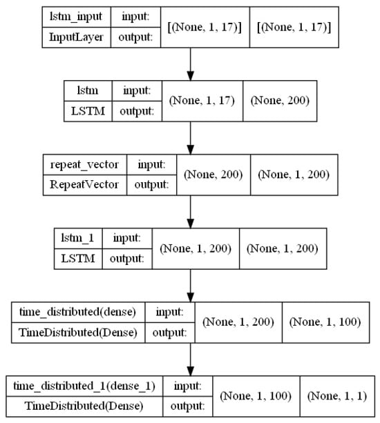
Figure A2.
Encoder–decoder–LSTM architecture.
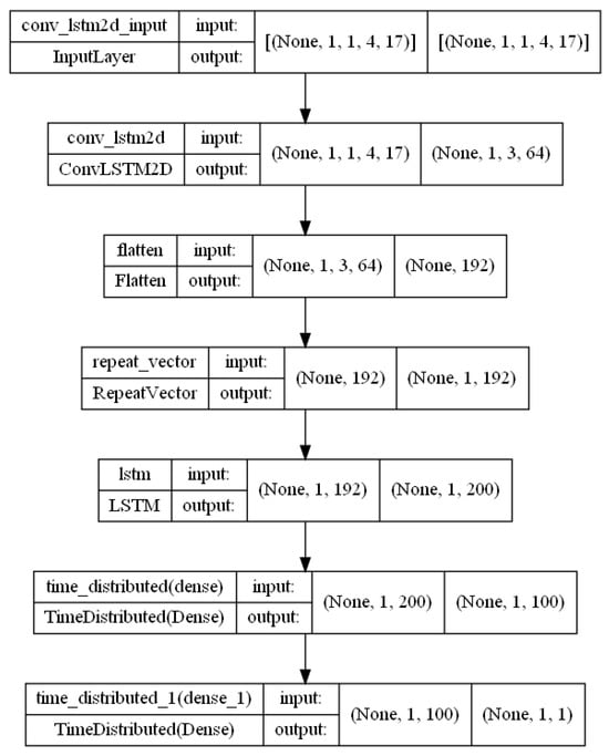
Figure A3.
Conv–LSTM architecture.
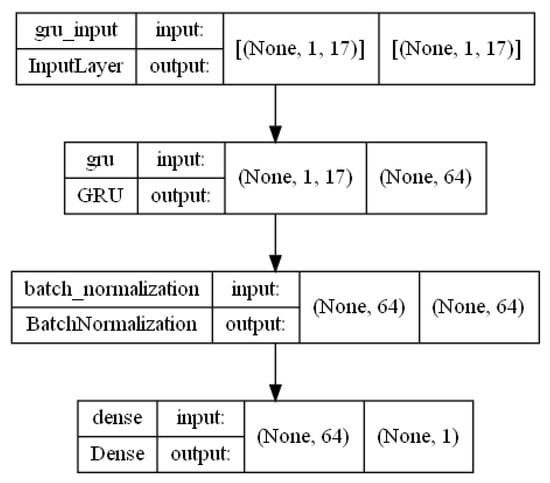
Figure A4.
GRU architecture.
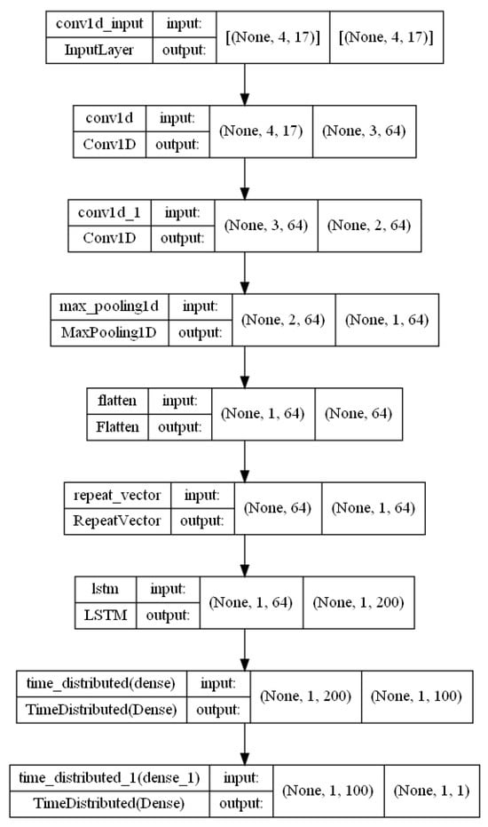
Figure A5.
CNN–encoder–decoder–LSTM architecture.
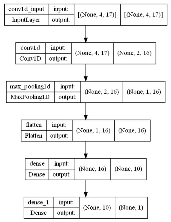
Figure A6.
CNN architecture.
Appendix A.2. Wind
This subchapter presents visualizations of proposed hybrid architectures of wind farms for a time horizon of 1 h.
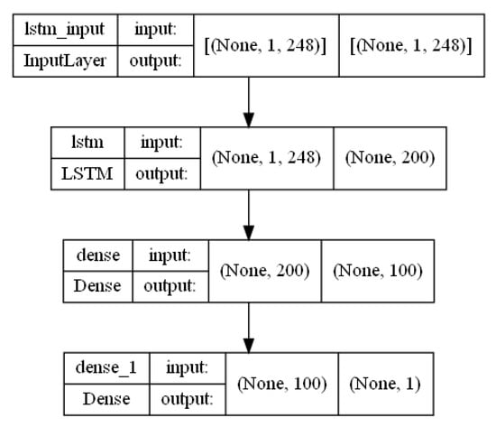
Figure A7.
Multi-LSTM architecture.
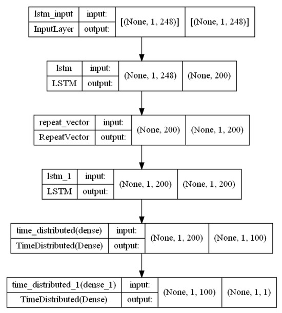
Figure A8.
Encoder–decoder–LSTM architecture.
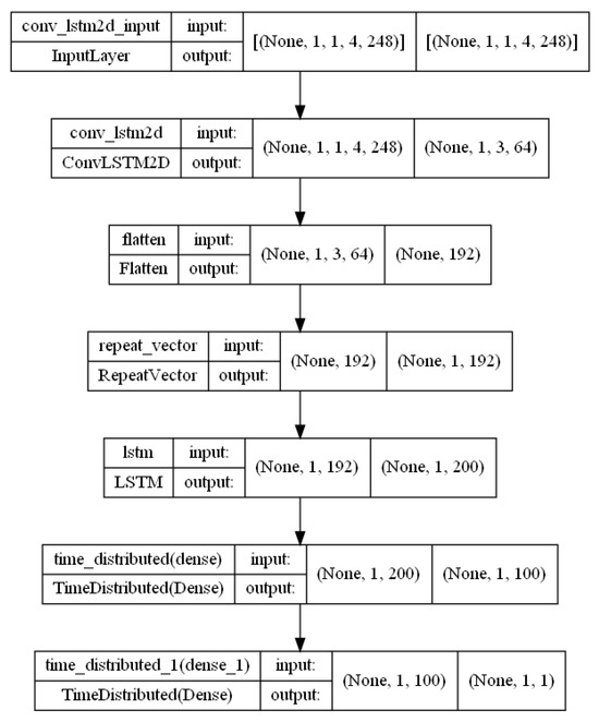
Figure A9.
Conv–LSTM architecture.
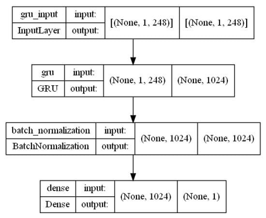
Figure A10.
GRU architecture.
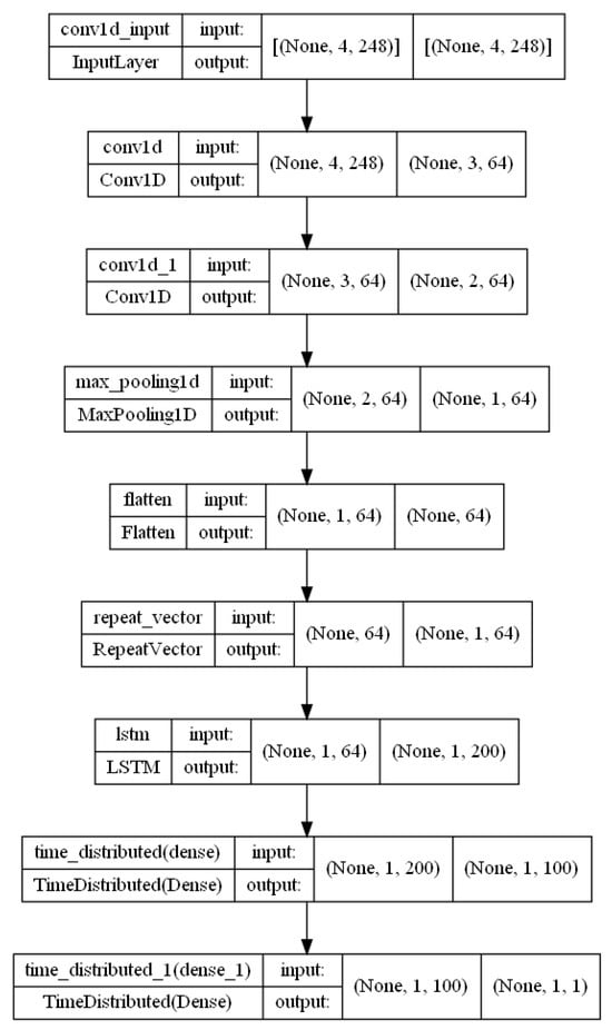
Figure A11.
CNN–encoder–decoder–LSTM architecture.
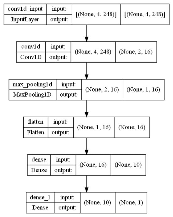
Figure A12.
CNN architecture.
Appendix B. Visualization PV
This subchapter presents visualizations of the operation of the best model for individual PV farms for a time horizon of 1 h. In the graphs, the prediction of the trained model is shown in green/brown, and the original value in blue.
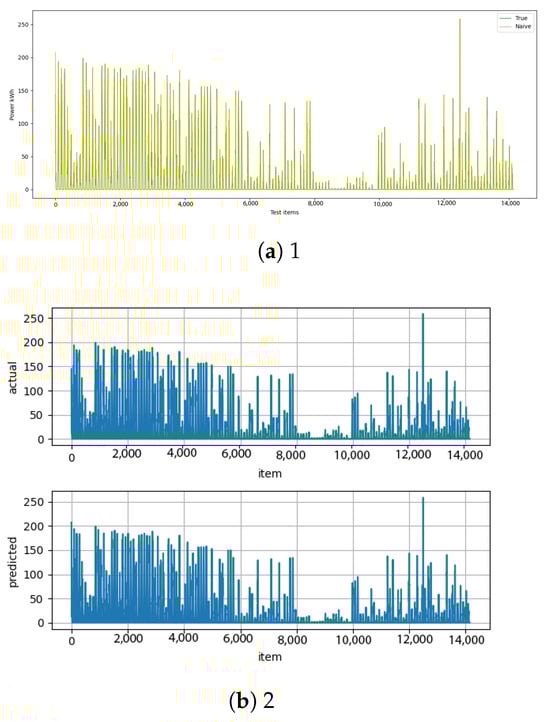
Figure A13.
Naive [13] and naive–diff [14] results.
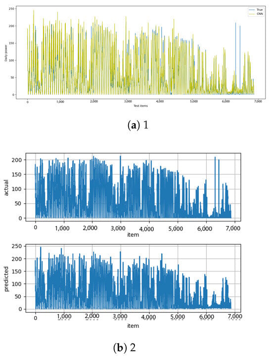
Figure A14.
CNN [13] and CNN–diff [14] results.
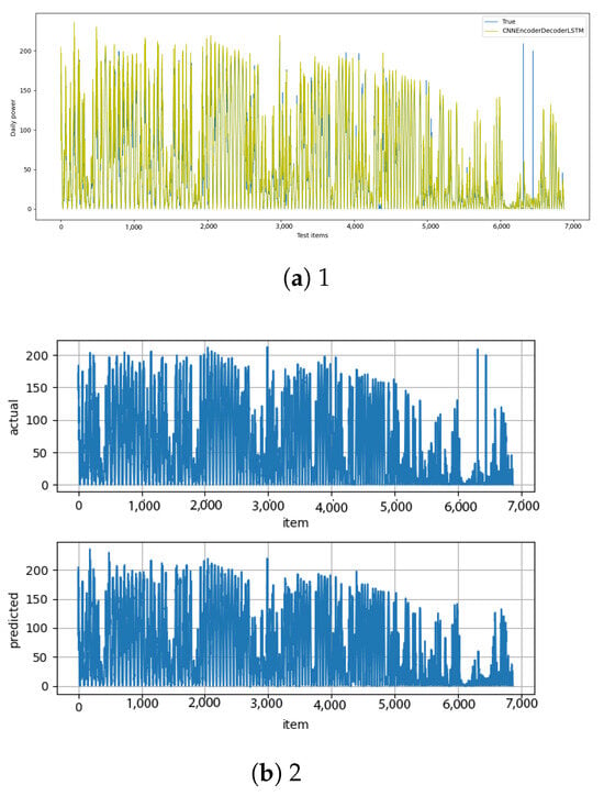
Figure A15.
CNN–encoder–decoder–LSTM [13] and CNN–encoder–decoder–LSTM–diff [14] results.
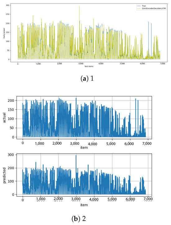
Figure A16.
Conv–encoder–decoder–LSTM [13] and conv–encoder–decoder–LSTM–diff [14] results.
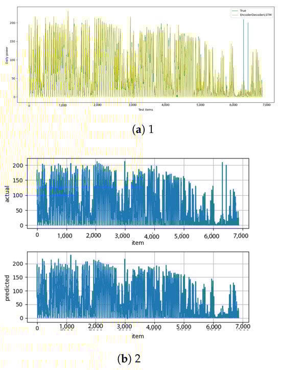
Figure A17.
Encoder–decoder–LSTM [13] and encoder–decoder–LSTM–diff [14] results.
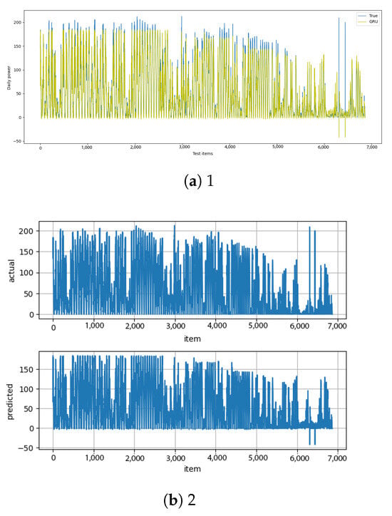
Figure A18.
GRU [13] and GRU–diff [14] results.
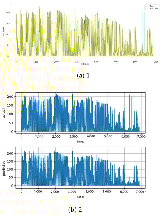
Figure A19.
Multi-LSTM [13] and multi-LSTM–diff [14] results.
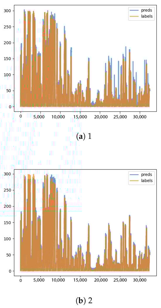
Figure A20.
TSPP LSTM [13] and TSPP TFT [14] results.
Appendix C. Visualization of Wind
This subchapter presents visualizations of the operation of the best models for individual wind farms for a time horizon of 1 h. In the graphs, the prediction of the trained model is shown in green/brown, and the original value in blue.
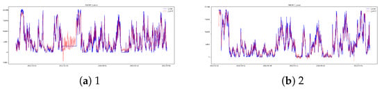
Figure A21.
Lasso EW3 [13,14] results.
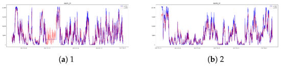
Figure A22.
RF EW3 [13,14] results.
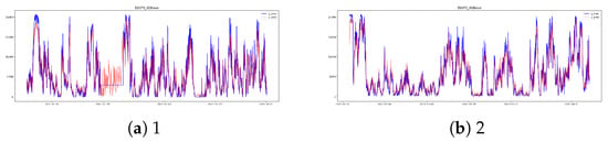
Figure A23.
XgBoost EW3 [13,14] results.
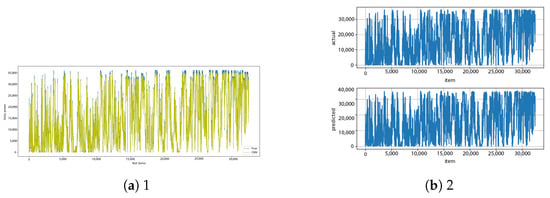
Figure A24.
CNN [13] and CNN–diff [14] results.
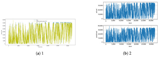
Figure A25.
CNN–encoder–decoder–LSTM [13] and CNN–encoder–decoder–LSTM–diff [14] results.
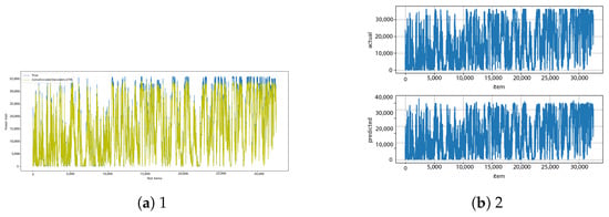
Figure A26.
Conv–encoder–decoder–LSTM [13] and conv–encoder–decoder–LSTM–diff [14] results.
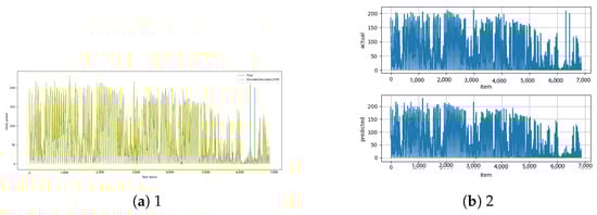
Figure A27.
Encoder–decoder–LSTM [13] and encoder–decoder–LSTM–diff [14] results.
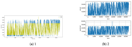
Figure A28.
GRU [13] and GRU–diff [14] results.
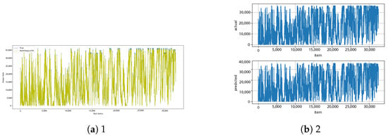
Figure A29.
Multi-LSTM [13] and multi-LSTM–diff [14] results.
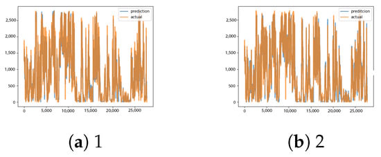
Figure A30.
EW1 LSTM [13] and TFT [14] results.
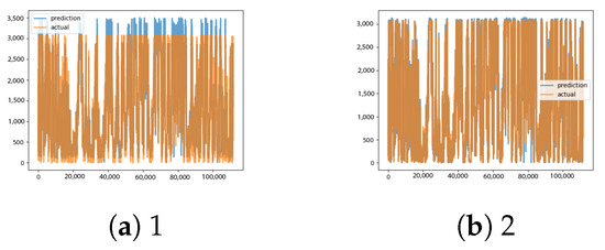
Figure A31.
EW2 LSTM [13] and TFT [14] results.
References
- Luo, X.; Zhang, D.; Zhu, X. Deep learning based forecasting of photovoltaic power generation by incorporating domain knowledge. Energy 2021, 225, 120240. [Google Scholar] [CrossRef]
- Bochenek, B.; Jurasz, J.; Jaczewski, A.; Stachura, G.; Sekuła, P.; Strzyżewski, T.; Wdowikowski, M.; Figurski, M. Day-Ahead Wind Power Forecasting in Poland Based on Numerical Weather Prediction. Energies 2021, 14, 2164. [Google Scholar] [CrossRef]
- Wen, J.; Li, Y.; Li, Y.; Zhang, Y. Short-Term Load Forecasting for Electrical Power Distribution Systems Using Enhanced Deep Neural Networks. USN Open Arch. 2018, 186856–186871. [Google Scholar] [CrossRef]
- Liu, J.; Wang, Y. Power Grid Fault Diagnosis Method Based on VGG Network Line Graph Semantic Extraction. Int. J. Sci. Eng. Res. 2022, 10, 16–20. Available online: https://www.ijser.in/archives/v10i5/SE22502172124.pdf (accessed on 27 May 2025). [CrossRef]
- Graves, A. Generating Sequences With Recurrent Neural Networks. arXiv 2013, arXiv:1308.0850. [Google Scholar]
- Zhang, Y.; Zhang, Y. CLVSA: A Convolutional LSTM Based Variational Sequence-to-Sequence Model with Attention for Predicting Trends of Financial Markets. arXiv 2019, arXiv:2104.04041. [Google Scholar]
- Chung, J.; Gulcehre, C.; Cho, K.; Bengio, Y. Empirical Evaluation of Gated Recurrent Neural Networks on Sequence Modeling. arXiv 2014, arXiv:1412.3555. [Google Scholar]
- Liu, Y.; Wang, Y.; Liu, Y. Methods of Forecasting Electric Energy Consumption: A Literature Review. Energies 2019, 15, 8919. [Google Scholar]
- Chen, W.; Zhang, L.; Liu, L.; Lin, Z.; He, D.; Chen, J. Photovoltaic Power Generation Forecasting Based on Secondary Data Decomposition and Hybrid Deep Learning Model. Energies 2021, 18, 3136. [Google Scholar]
- Huang, H.; Castruccio, S.; Genton, M.G. Forecasting High-Frequency Spatio-Temporal Wind Power with Dimensionally Reduced Echo State Networks. J. R. Stat. Soc. Ser. Appl. Stat. 2022, 71, 449–466. [Google Scholar] [CrossRef]
- Bilski, J.; Rutkowski, L.; Smolag, J.; Tao, D. A novel method for speed training acceleration of recurrent neural networks. Inf. Sci. 2021, 553, 266–279. [Google Scholar] [CrossRef]
- Time Series Forecasting with the NVIDIA Time Series Prediction Platform and Triton Inference Server. NVIDIA Developer Blog. Available online: https://developer.nvidia.com/blog/time-series-forecasting-with-the-nvidia-time-series-prediction-platform-and-triton-inference-server/ (accessed on 16 June 2025).
- Sahu, A.K.; Zhao, S.; Xu, Z.; Zhu, Z.; Liang, X.; Zhang, Z.; Jiang, R. Short and Long-Term Renewable Electricity Demand Forecasting Based on CNN-Bi-GRU Model. IECE Trans. Emerg. Top. Artif. Intell. 2025, 2, 1–15. [Google Scholar]
- Almarzooqi, A.M.; Maalouf, M.; El-Fouly, T.H.M.; Katzourakis, V.E.; El Moursi, M.S.; Chrysikopoulos, C.V. A hybrid machine-learning model for solar irradiance forecasting. Clean Energy 2024, 8, 100–110. [Google Scholar] [CrossRef]
- Salman, D.; Direkoglu, C.; Kusaf, M.; Fahrioglu, M. Hybrid deep learning models for time series forecasting of solar power. Neural Comput. Appl. 2024, 36, 9095–9112. [Google Scholar] [CrossRef]
- Lim, B.; Arik, S.Ö.; Loeff, N.; Pfister, T. Temporal Fusion Transformers for Interpretable Multi-horizon Time Series Forecasting. arXiv 2021, arXiv:1912.09363. [Google Scholar] [CrossRef]
- Tadeusiewicz, R.; Chaki, R.; Chaki, N. Exploring Neural Networks with C#; CRC Press: Boca Raton, FL, USA, 2014. [Google Scholar]
- Stefanowski, J.; Krawiec, K.; Wrembel, R. Exploring complex and big data. Int. J. Appl. Math. Comput. Sci. 2017, 27, 669–679. [Google Scholar] [CrossRef]
- Qadir, Z.; Khan, S.I.; Khalaji, E.; Munawar, H.S.; Al-Turjman, F.; Mahmud, M.A.P.; Kouzani, A.Z.; Le, K. Predicting the energy output of hybrid PV–wind renewable energy system using feature selection technique for smart grids. Energy Rep. 2021, 7, 8465–8475. [Google Scholar] [CrossRef]
- Demirkiran, M.; Karakaya, A. Efficiency analysis of photovoltaic systems installed in different geographical locations. Open Chem. 2022, 20, 748–758. [Google Scholar] [CrossRef]
- Roberts, J.; Cassula, A.; Freire, J.; Prado, P. Simulation and Validation Of Photovoltaic System Performance Models. In Proceedings of the XI Latin-American Congress on Electricity Generation and Transmission–CLAGTEE 2015, Sao Paulo, Brazil, 8–11 November 2015. [Google Scholar]
- Milosavljević, D.D.; Kevkić, T.S.; Jovanović, S.J. Review and validation of photovoltaic solar simulation tools/software based on case study. Open Phys. 2022, 20, 431–451. [Google Scholar] [CrossRef]
- Wang, B.; Wang, X.; Wang, N.; Javaheri, Z.; Moghadamnejad, N.; Abedi, M. Machine learning optimization model for reducing the electricity loads in residential energy forecasting. Sustain. Comput. Inform. Syst. 2023, 38, 100876. [Google Scholar] [CrossRef]
- Ma, H.; Xu, L.; Javaheri, Z.; Moghadamnejad, N.; Abedi, M. Reducing the consumption of household systems using hybrid deep learning techniques. Sustain. Comput. Inform. Syst. 2023, 38, 100874. [Google Scholar] [CrossRef]
- Wang, X.; Zhu, W. Advances in neural architecture search. Natl. Sci. Rev. 2024, 11, nwae282. [Google Scholar] [CrossRef] [PubMed]
- Aksoy, N.; Yılmaz, A.; Bayrak, G.; Koç, M. Deep learning approaches for robust prediction of large-scale renewable energy generation: A comprehensive comparative study from a national context. Intell. Data Anal. 2025. [Google Scholar] [CrossRef]
- Sarkar, K. Load and Renewable Energy Forecasting Using Deep Learning for Grid Stability. arXiv 2025, arXiv:2501.13412. [Google Scholar]
- Sua, L.; Wang, H.; Huang, J. Deep Learning in Renewable Energy Forecasting: A Cross-Dataset Evaluation of Temporal and Spatial Models. arXiv 2025, arXiv:2505.03109. [Google Scholar]
Disclaimer/Publisher’s Note: The statements, opinions and data contained in all publications are solely those of the individual author(s) and contributor(s) and not of MDPI and/or the editor(s). MDPI and/or the editor(s) disclaim responsibility for any injury to people or property resulting from any ideas, methods, instructions or products referred to in the content. |
© 2025 by the authors. Licensee MDPI, Basel, Switzerland. This article is an open access article distributed under the terms and conditions of the Creative Commons Attribution (CC BY) license (https://creativecommons.org/licenses/by/4.0/).