Experimental Study and CFD Analysis of a Steam Turbogenerator Based on a Jet Turbine

Abstract

Implementing energy-efficient solutions and developing energy complexes to decentralise power supply are key objectives for enhancing national security in Ukraine and Eastern Europe. This study compares the design, numerical, and experimental parameters of a channel-type jet-reaction turbine. A steam turbogenerator unit and a pilot industrial experimental test bench were developed to conduct full-scale testing of the unit. The article presents experimental data on the operation of a steam turbogenerator unit with a capacity of up to 475 kW, based on a channel-type steam jet-reaction turbine (JRT), and includes the validation of a computational fluid dynamics (CFD) model against the obtained results. For testing, a pilot-scale experimental facility and a turbogenerator were developed. The turbogenerator consists of two parallel-mounted JRTs operating on a single electric generator. During experimental testing, the system achieved an electrical output power of 404 kW at a turbine rotor speed of 25,000 rpm. Numerical modelling of the steam flow in the flow path of the jet-reaction turbine was performed using ANSYS CFX 25 R1 software. The geometry and mesh setup were described, boundary conditions were defined, and computational calculations were performed. The experimental results were compared with those obtained from numerical simulations. In particular, the discrepancy in the determination of the power and torque on the shaft of the jet-reaction turbine between the numerical and full-scale experimental results was 1.6%, and the discrepancy in determining the mass flow rate of steam at the turbine inlet was 1.34%. JRTs show strong potential for the development of energy-efficient, low-power turbogenerators. The research results confirm the feasibility of using such units for decentralised energy supply and recovering secondary energy resources. This contributes to improved energy security, reduces environmental impact, and supports sustainable development goals.

1. Introduction

In the modern world, there is growing interest in transforming energy systems to enhance their efficiency, reliability, and environmental sustainability. Decentralised energy production and the integration of renewable energy sources are central to this transformation. These approaches are considered key strategies for reducing greenhouse gas emissions, enhancing the reliability of the power supply, and lowering energy costs. The international scientific community has long explored the decentralisation of energy production [1], the integration of renewable energy into urban infrastructure [1], and the potential drawbacks of these innovations despite their undeniable advantages [2].

According to Ukraine’s Energy Strategy through 2050, one of the priorities is the decentralisation of electricity generation across the country to improve the stability and reliability of the energy supply system [3]. As international experience shows [4], the saturation of the economy with independent distributed energy sources leads to reduced energy costs, increased competitiveness of enterprises, and enhanced national energy security, additionally aligning with the goals of sustainable development.

Innovations in mechanical engineering continue to generate and refine promising solutions in turbine technology. Developing new designs or upgrading existing turbine units [5] requires a deep understanding of the physical processes occurring in the flow paths of turbomachinery. Researchers can investigate these processes using classical methods, such as experimental or model testing [6], as well as modern approaches—namely, simulation using computational software packages [7]. In both cases, the results should validate the accuracy and reliability of the theoretical models. When designing new systems, it is crucial to establish a solid foundation through experimental or full-scale tests, which subsequently becomes the basis for a faster and more cost-effective development method—numerical simulation.

A potential solution for decentralising the energy system and supplying small-to medium-sized consumers is deploying turbine-based power systems with capacities up to 500 kW. Gas turbine units typically include a compressor, turbine, inverter, and recuperator. Although such systems tend to operate with relatively low efficiency, their primary drawback lies in the reliance on fossil-based fuels such as natural or associated gas, or on limited resources like biogas. There are methods to improve the efficiency of these systems. However, using additional resources is costly and not always feasible, and in any case, combustion products are generated during operation, negatively impacting the environment [8].

A more environmentally friendly solution is proposed in a study [9], which suggests replacing throttle valves with turboexpanders and integrating solar heating systems into the natural gas pressure reduction process at gas distribution stations. This approach improves the overall efficiency of the stations without causing environmental harm. However, such equipment can be installed only at gas distribution stations and is intended solely for on-site power generation.

An innovative and increasingly promising direction involves using turbine systems based on vortex and jet-reaction turbines (JRTs). This turbine type has been successfully applied in the energy sector, particularly for developing small-scale turbogenerators (up to 500 kW) powered by compressed gas energy. Studies [10,11] present examples of such systems, demonstrating their structural simplicity and capability to supply electricity to industrial or municipal consumers.

Experimental and full-scale studies are expensive to develop and conduct, yet they are crucial in verifying theoretical models and computational simulations. This is because their results do not depend on assumptions inherent to theoretical models, which may contain potential errors, and are not limited by the functionality of software tools. Positive experience has already been gained in building experimental test benches and conducting trials [12]. However, these studies have several disadvantages: high capital costs for equipment manufacturing and refinement, long setup and testing durations, the requirement for dedicated laboratory space, and significant challenges in observing physical processes inside the flow path. Given these limitations, numerical simulation is a more practical approach for analysing internal turbine processes and optimising their design. Successful examples of combining experimental studies with numerical modelling are presented in work such as [13].

This study aims to compare the numerical and experimental parameters and to investigate steam flow within the flow path of a channel-type jet-reaction turbine.

The main tasks include

• obtaining and analysing experimental test results of the prototype steam turbogenerator unit STGU-JRT-475-24/0.5 based on the JRT;
• conducting numerical simulation of steam flow within the flow path of the JRT using the ANSYS CFX software suite;
• analysing the data obtained through numerical simulations;
• comparing the results of numerical modelling with the results from experimental testing
• assessing the feasibility of further research and modernisation of the channel-type JRT.

The main research gap addressed by this study lies in the lack of experimentally validated data for this type of turbine, which features an innovative design with a fixed inlet nozzle and a disk-type channel impeller. Although theoretical models and calculation methods exist, open sources lack experimental data from full-scale units operating under real conditions and simulation results for turbines using modern CFD software. This significantly limits the understanding of the complex internal flow phenomena and hinders the optimisation of turbine designs. The present study addresses this issue by developing a pilot-scale industrial test facility, acquiring benchmark experimental data, and conducting validated numerical simulations using ANSYS CFX 25 R1 software.

2. Research Methodology

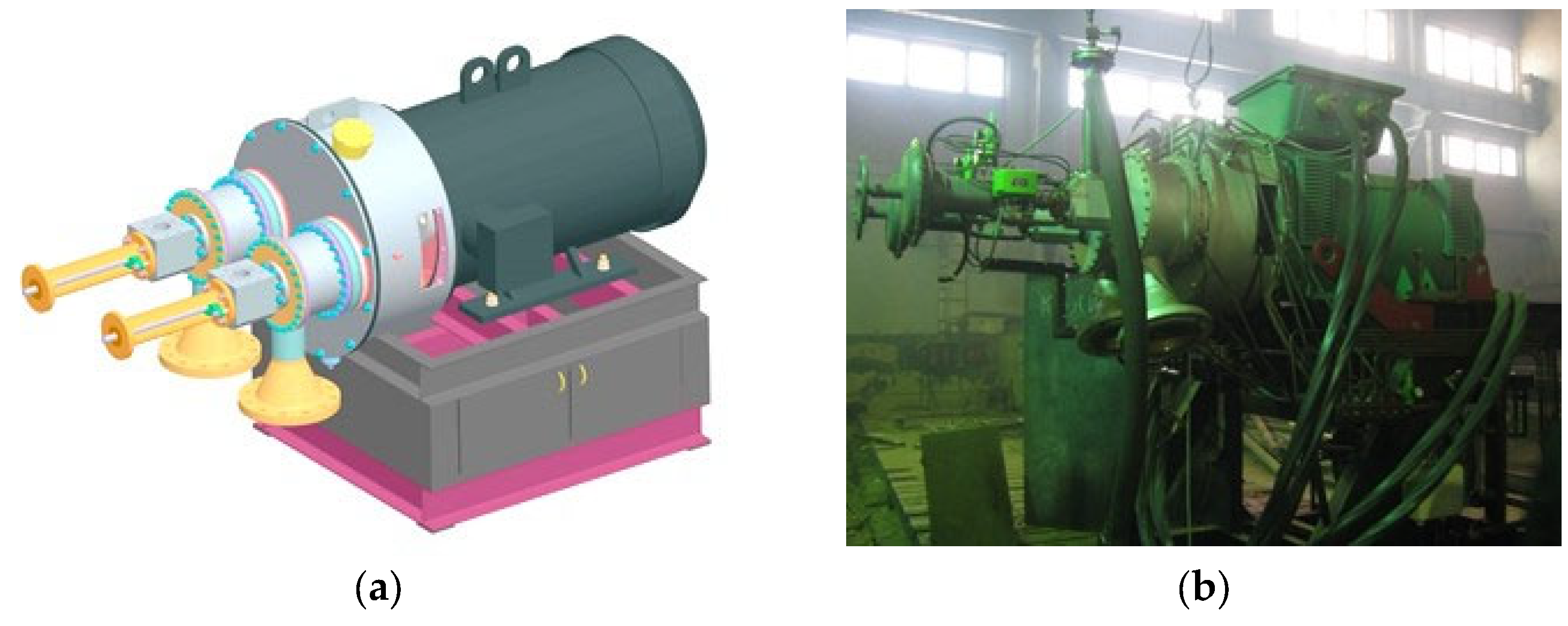
2.1. Experimental Stand

The steam turbogenerator unit STGU-JRT-475-24/0.5 and a pilot-scale experimental test bench were developed and manufactured at LLC “UKRNAFTOZAPCHASTYNA” (Sumy, Ukraine). The test bench was installed at PJSC “SUMYKHIMPROM” (Sumy, Ukraine). Figure 1 and Figure 2 show the external view of the test bench and its schematic diagram, respectively.

The main components of the test bench include

• steam and air supply pipelines;
• the pipeline system of the bench, along with shut-off and control valves;
• a flowmeter;
• a steam turbogenerator unit (STGU) based on a JRT;
• an electric generator;
• an information and measurement system for recording the working fluid flow rate, active electrical power, rotor speed, and the pressures and temperatures at the inlet and outlet of the unit.

Waste-heat boilers generate steam in the furnace section of the sulfuric acid department at PJSC “SUMYKHIMPROM” with the following parameters: pressure—4 MPa, temperature—450 °C. The steam is delivered through a supply pipeline to a hand regulating device (HRD), where water is injected to reduce the steam parameters to a pressure of up to 2.43 MPa and a temperature of up to 350 °C. The working fluid then flows through a flowmeter and into the regulating nozzles of the STGU. These nozzles regulate the steam’s mass flow rate before it enters the axial channel of the JRT, which consists of a cylindrical axial section and a diffuser section. Inside the axial channel of the rotor, the steam flow decelerates as it passes through a shock wave to subsonic speed. It continues to move through the flow path at a low velocity and with minimal energy losses until it reaches the thrust nozzles. The steam exits these nozzles at supersonic speed, generating reactive thrust and torque on the turbine shaft. Mechanical work is performed as the shaft rotates.

The STGU-JRT-475-24/0.5 is a base model for a series of steam turbogenerator units using JRTs with capacities of 160, 250, 315, and 475 kW. These units are designed to generate electricity by converting the potential energy of steam pressure released during expansion in the JRT into mechanical energy on the generator shaft, and subsequently into electrical power.

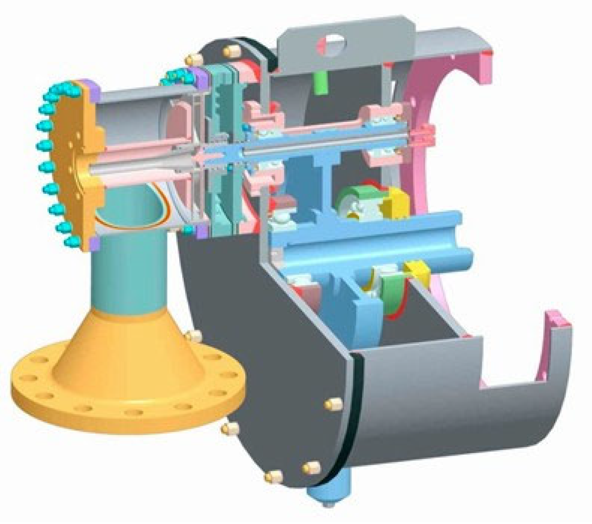
The STGU-JRT-475-24/0.5 features two JRTs, each rated at 250 kW, mounted in parallel, and connected to a single 475 kW electric generator (400 V, 50 Hz) via a single-stage gear reducer. The 3D models and a general cross-sectional view of the JRT and the gear reducer are shown in Figure 3 and Figure 4.

The output shaft of the gear reducer connects to a generator with a rated power of 475 kW. The exhaust steam is directed to a deaerator or discharged into the atmosphere during emergencies. The experimental test bench has a compressed air supply system for purging.

A set of control and computational instruments was installed to obtain measurement data on the operating parameters of the STGU and monitor its condition. This system enables

• real-time monitoring of all test bench systems;
• measurement of total power output of generated electrical energy;
• recording and storage of measurement data;
• graphical representation of measured parameters.

The test bench has sensors for monitoring pressure, temperature, generator rotational speed, electrical power output, and vibration levels.

All necessary parameters were measured during the experimental studies, including the pressures and temperatures required for conducting numerical simulations and validating their results (

Table 1. List of monitored pressure and temperature parameters of the test bench.

Parameter Name	Measurement Range	Measurement Error, %	Sensor Type
Steam pressure at the inlet, MPa	0…2.5	0.25	WIKA S-10 990 34 G ½ KN3.2
Steam pressure at the outlet, MPa	−0.1…0.6	0.25	WIKA S-10 990 34 G ½ KN3.2
Pressure drops across the orifice plate, MPa	0…0.1
Steam temperature at the inlet, °C	0…400	0.25	TSPU 1-3-100P-V-2-80-8-70-D
Steam temperature at the outlet, °C	0…300	0.25	TSPU 1-3-100P-V-2-80-8-70-D

).

The electrical parameters of the generator monitors are measured using the multifunctional device SATEC PM130P and the “Indigo+” electric energy meter. The SATEC PM130P is a three-phase instrument designed to measure the main electrical network parameters and record and store data.

Table 2. List of monitored electrical parameters.

Parameter Name	Measurement Range	Measurement Error, %
Electrical power, kW	0…500	±0.3
Frequency, Hz	45…65	±0.02
Voltage, V	300…450	±0.2
Current, A	0…1000	±0.2
Energy amount, kWh		±0.2

lists the measured electrical parameters and their measurement ranges.

The shaft rotational speed of the generator was monitored using the tachometric transducer IT14.14.000, which has a measurement range from 0 to 5000 rpm and a measurement error of 1%.

Before the commencement of testing, the availability of the following documents was verified:

• a certificate of quality or calibration certificate for all instruments;
• a readiness report for the industrial test bench, including assessment of installation feasibility;
• quality control department acceptance reports for the STGU-JRT-475-24/0.5 and its assembly units;
• test protocols for the electrical systems and equipment of the STGU-JRT-475-24/0.5, conducted after its installation on the pilot-scale industrial test bench;
• Test protocols for the instrumentation and control equipment of the STGU-JRT-475-24/0.5 after installation.

Testing was carried out according to the developed program and methodology for preliminary tests of the STGU-JRT-475-24/0.5.

The design specifications of the unit for the nominal operating mode are as follows:

• inlet steam gauge pressure to the JRT: 2.43 MPa;
• inlet steam temperature to the JRT: 350 °C;
• outlet steam gauge pressure from the JRT: 0.05 MPa;
• steam mass flow rate: 7.8 t/h;
• electrical power: 475 kW.

The unit operated at modes of up to 505 kW during testing. The unit’s operating parameters (pressure and temperature) remained within permissible ranges in all operating modes. The vibration and temperature conditions of the bearings were within normal limits.

The errors of direct measurements are classified as systematic or random. To reduce random errors, a series of repeated measurements was performed. Systematic errors include instrumental, positional, and subjective components. Positional errors were minimised by adhering to the manufacturer’s installation guidelines for instruments and equipment. Instrumental errors are determined by the accuracy class and resolution of the instruments, as well as compliance with operational procedures. Subjective errors were mitigated by having multiple researchers repeat the measurements independently.

When processing the test results and determining the uncertainty of indirect measurements, it was assumed that the distribution of measurement errors follows a customary (Gaussian) law. This assumption is justified since indirect measurements are functions of multiple independent variables. According to the central limit theorem, if the total error arises from the combined effect of many independent factors, each contributing only marginally to the overall uncertainty, their cumulative effect can be approximated by a normal distribution.

Multiple measurements were taken for each monitored quantity during testing. The arithmetic mean was then calculated, for example, for the gas pressure at the inlet to the JRT:

$$\overline{P_H}={\displaystyle \frac{\sum _{i=1}^M{P}_H}{n}},$$

(1)

Then, the root mean square error of the measurement result was calculated as

$$S_{P_H}=\sqrt{{\displaystyle \frac{\sum _{i=1}^M{\left(∆\overline{P_H}\right)}^2}{n·(n-1)}}},$$

(2)

where $∆\overline{P_H}=\overline{P_H}-P_H$ is error of the i-th measurement, and n is the number of measurements.

The absolute error of the indirect measurement result was determined using the following equation:

$$\delta y=\sqrt{\sum _{i=1}^M{\left({\displaystyle \frac{\partial y}{\partial x_i}}\right)}^2·{\left(\delta x_i\right)}^2},$$

(3)

The relative error of the result of the indirect measurement was then calculated as

$${\epsilon }_y={\displaystyle \frac{\delta y}{y}},$$

(4)

or

$${\epsilon }_y=\sqrt{{\sum }_{i=1}^M{\left({\displaystyle \frac{\partial }{{\partial x}_i}}\mathit{ln}y\right)}^2·{\left(\delta x_i\right)}^2}.$$

(5)

The processing of test results was carried out in accordance with the developed and approved methodology titled “Test Results of STGU-JRT-475-24/0.5 and Their Processing”, prepared by specialists from LLC “UKRNAFTOZAPCHASTYNA”.

According to the developed and approved test program and methodology, only data obtained under stable operating conditions of the unit over an agreed-upon period of time were accepted for processing. This corresponded to the regime with an output power of 404 kW.

An operating mode with a power output of 404 kW was selected for comparison with the numerical modelling results. For this mode,

• inlet steam gauge pressure to the JRT: 1.8224 MPa;
• inlet steam temperature to the JRT: 275.5 °C;
• outlet steam gauge pressure from the JRT: 0 Pa;
• outlet steam temperature: 146.4 °C.

In this mode, the electrical power of the STGU was 404 kW, the steam mass flow rate was 7.577 t/h, and the JRT rotor speed was 25,000 rpm.

2.2. Numerical Simulations

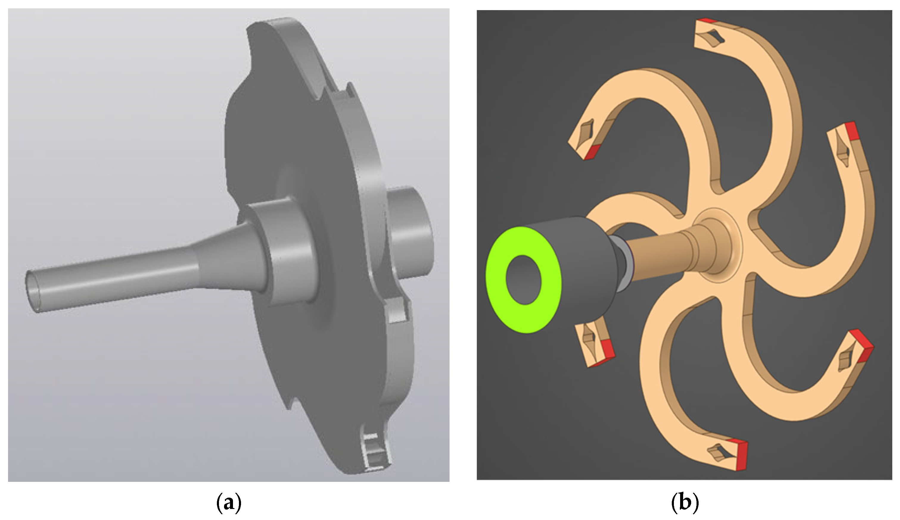
Numerical simulation of steam flow within the flow path of the JRT was performed using the ANSYS CFX software package.

A solid 3D model of the JRT impeller is shown in Figure 5a. The three-dimensional model of the computational domain of the investigated sample represents the internal volume of the JRT flow passage and is shown in Figure 5b. The domain is divided into stator and rotor regions, with a clearance gap separating them. The stator region is bounded at the inlet by a supply sleeve (green area in Figure 5b), while the rotor region begins downstream of the nozzle section of the rotor wheel (red areas in Figure 5b).

The overall geometric dimensions of the computational domain, which represent the actual dimensions of the JRT, are provided in

Table 3. Overall geometric dimensions.

Region	Geometric Dimensions, mm
Outer diameter of the rotor	267
Outer diameter of the stator	65
Axial length of the domain	223.8
Clearance between stator and rotor	0.7

.

A hybrid computational mesh was generated for the simulations, combining various types of elements selected based on the geometric complexity of different regions and the required modelling accuracy [14,15]. The mesh includes the following cell types:

• Tetrahedral elements: These four-faced elements are suitable for complex and irregular geometries. They provide high accuracy for domains with substantial shape variations, particularly in 3D geometries featuring numerous surfaces and edges.
• Wedge (prismatic) cells: These five-faced elements, composed of two triangular and three quadrilateral faces, are commonly used for simulating wedge-shaped regions. They effectively capture flow parameter variations in expanding or contracting channel sections.
• Pyramidal cells: These elements, also five-faced, are typically applied in transition zones between regions with different element types. They ensure a smooth transition between fine and coarse mesh areas, which is crucial for capturing flow gradients in critical zones, such as peripheral regions or areas with steep velocity and pressure changes.

Mesh refinement was applied in the boundary layer regions to enhance calculation accuracy (Figure 6a,b). It allowed for more accurate resolution of temperature, pressure, and velocity gradients near the domain walls. Additional local mesh refinement was applied around the thrust nozzles of the impeller (Figure 6c) to better capture the flow characteristics in this critical region. Furthermore, mesh densification was implemented in the clearance gap between the stator and rotor (Figure 6d).

Before initiating the numerical simulations, a mesh independence study was conducted to evaluate the effect of mesh resolution on result accuracy. Simulations were performed using four different mesh configurations with varying element counts, as presented in

Table 4. Mesh independence study results.

No.	Number of Cells, Millions of Pcs.			Mass Flow, kg/s			Torque, N·m	Min. Y+ Value	Min Mesh Quality	Average Orthogonal Quality
	Stator	Rotor	Total	Inlet	Outlet	Error, %
1	0.19	5.292	5.482	1.02918	1.01487	1.39	80.84	4.68	0.0013	0.677
2	1.56	10.33	11.89	1.03865	1.03052	0.78	82.17	2.17	0.0055	0.677
3	3.453	12.699	16.152	1.03851	1.03107	0.56	82.9	1.58	0.0225	0.794
4	4.187	17.44	21.627	1.03715	1.02917	0.57	82.95	1.53	0.0304	0.815

. As shown in Table 4, the four mesh variants ranged in total element count from 5.482 million to 21.627 million. Simulations using these variants yielded results of sufficient accuracy. However, as the mesh density increased, so did the computational complexity, potentially introducing additional numerical errors and significantly increasing the computation time.

The relative error of the mass flow rate and torque value was used to analyse the independence of the results from mesh quality. The input data for configuring the simulations were based on results obtained during full-scale experimental tests, which also enabled the evaluation of discrepancies between numerical and experimental torque values. Additional parameters to assess mesh independence included dimensionless mesh quality indicators: Min. Y⁺ value, Min Mesh Quality, and Average Orthogonal Quality.

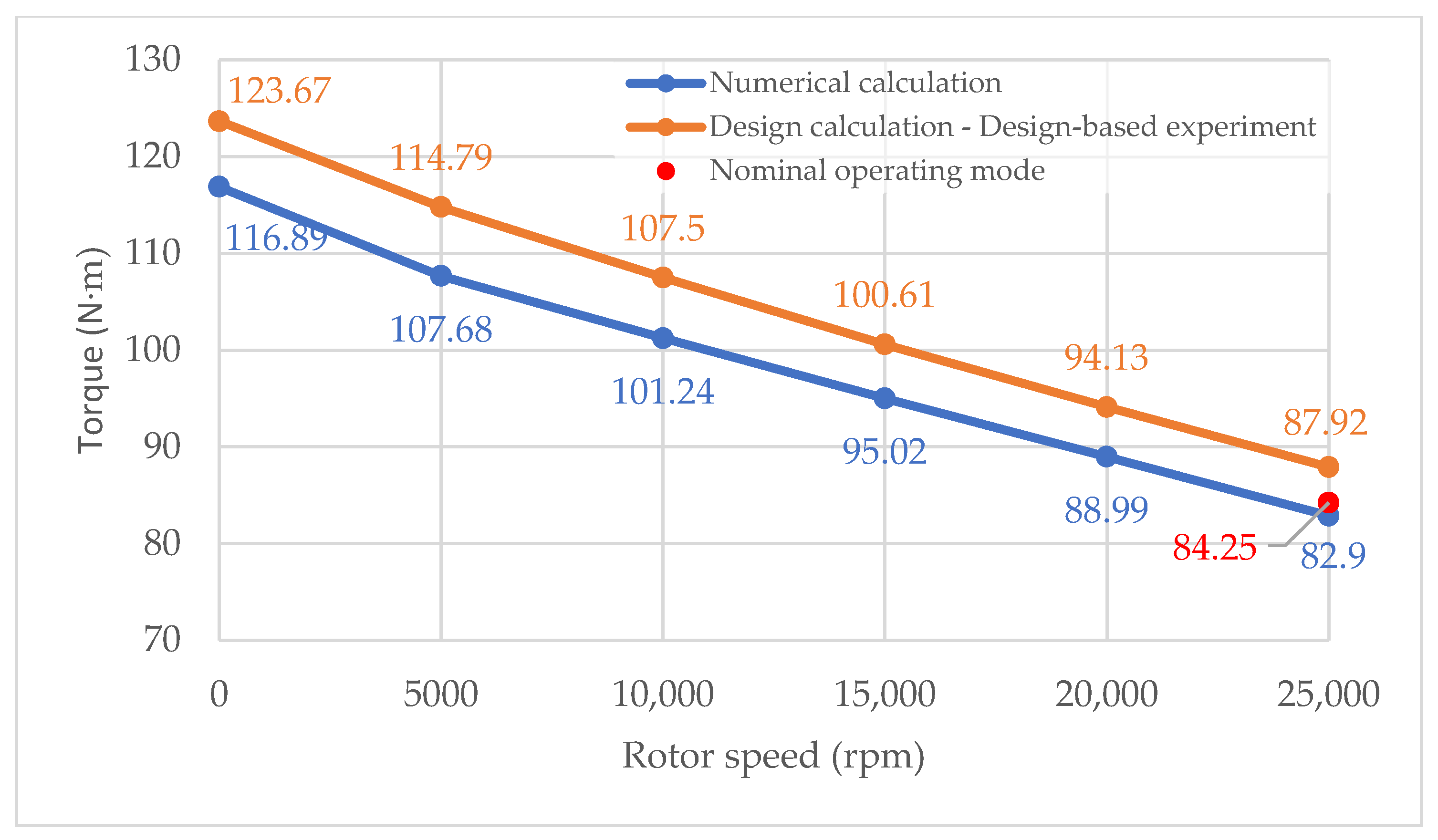
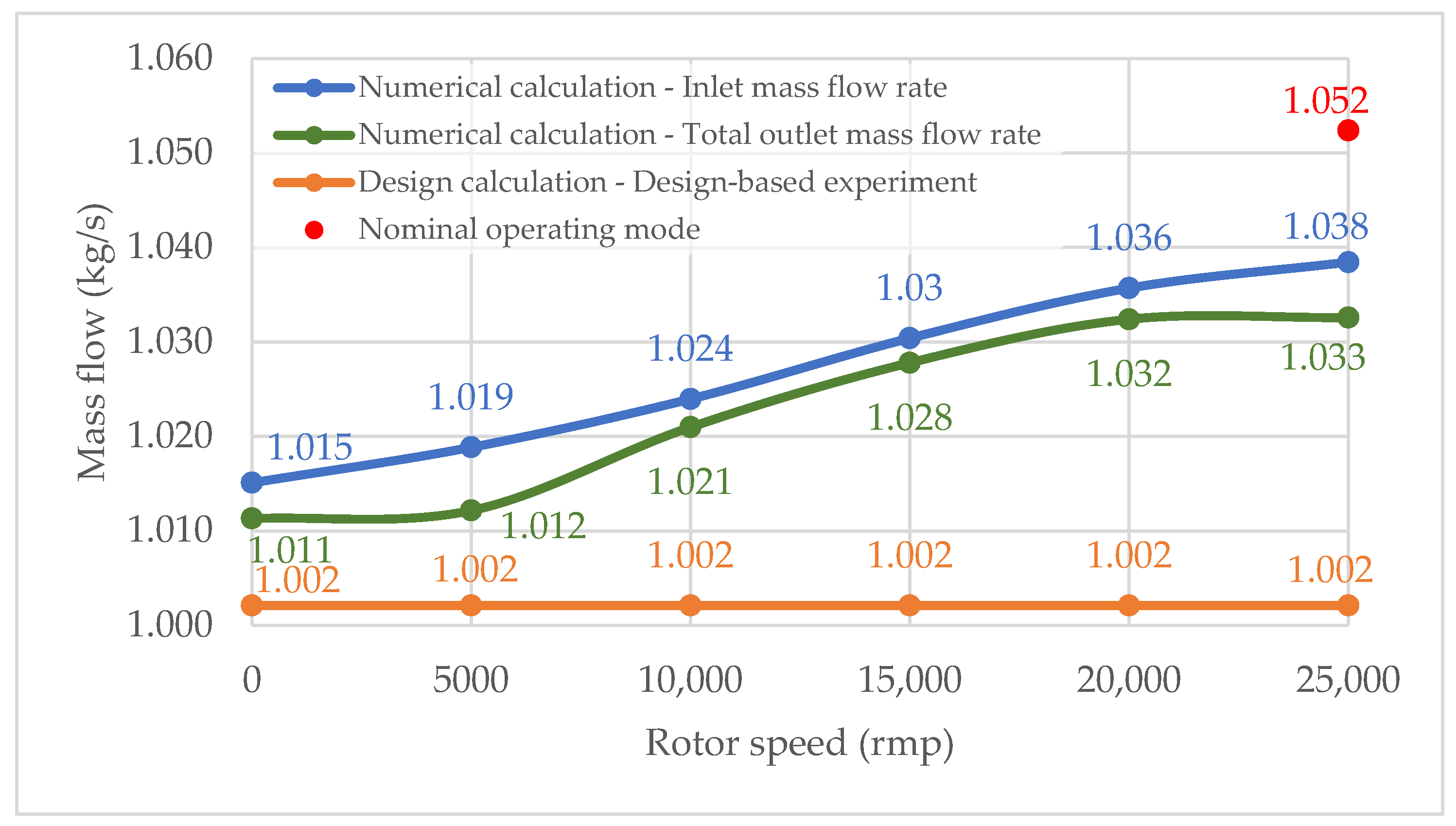
As shown in Table 4, the largest error in the calculated mass flow rate is observed for mesh variant 1, while the smallest errors are seen for variants 3 and 4. These variants also produce torque values closest to the experimental result (84.25 N·m), with a deviation not exceeding 1.6%. Additionally, for variants 3 and 4, the Min. Y⁺ value is less than 2, which is the lowest among all mesh configurations. The Average Orthogonal Quality exceeds 0.75, indicating high mesh quality.

For subsequent simulations, the mesh corresponding to Experiment No. 3 was selected, providing a mass flow rate error of 0.56% and a torque deviation of 1.6%. These values fall within the acceptable error margin and ensure an optimal balance between model accuracy and computational efficiency.

Detailed information about the computational mesh of the model is provided in

Table 5. Final mesh structure and cell counts.

Computational Region	Cell Type	Number of Cells, Millions of Pcs.
Stator	Tetrahedral	2.46
	Wedge (prism)	0.987
	Pyramidal	0.006
Rotor	Tetrahedral	2.573
	Wedge (prism)	10.113
	Pyramidal	0.013

.

The CFD simulation process comprises three main stages: pre-processing, processing, and post-processing. During the pre-processing stage, the computational domain is defined, and the input parameters for the simulation are specified, as summarised in

Table 6. Input parameters.

Parameter	Value
Machine type	Channel-type JRT
Working fluid	Steam
Reference pressure	151,325 kPa
Heat transfer model	Total Energy
Turbulence model	SST
Domain interface treatment	Frozen Rotor
Solver control > Advection scheme	High Resolution
Solver control > Timescale control	Auto timescale

. The numerical solution was carried out using ANSYS CFX software, while the CFD-Post module was used for post-processing and visualisation of the results.

Information about the thermophysical properties of the working fluid under initial conditions is provided in

Table 7. Thermophysical properties of the working fluid.

Property	Value
Density, kg/m3	7.620
Molar mass, kg/kmol	18.02
Specific heat capacity Cp, J/kg·K	2360
Specific heat capacity Cv, J/kg·K	1713
Thermal conductivity, W/m·K	0.04457
Dynamic viscosity, Pa·s	1.901·10−5

.

The use of the “Total Energy” heat transfer model enables accurate consideration of variations in density, temperature, and pressure typical of compressible flow.

The shear stress transport (SST) turbulence model was employed in this numerical study. This model combines the strengths of the k-ε and k-ω models to provide high accuracy in modelling the boundary layer. The SST model is particularly effective in predicting flow separation under adverse pressure gradients where turbulent flow dominates. By blending the two base models, SST accurately captures the entire boundary layer behaviour from the near-wall region to the outer edge. Moreover, it incorporates the Bradshaw assumption to improve separation prediction [16]. Its well-documented reliability and high accuracy justify the selection of the SST turbulence model in this study in simulating complex turbulent flows in turbomachinery, as well as its proven ability to accurately capture flow separation phenomena—a critical factor in hydrodynamic analysis of turbocompressors and other energy systems [17,18,19,20]. Its implementation enables the reliable prediction of flow behaviour, thereby enhancing the credibility of the simulation results for further analysis and design optimisation.

Moreover, in this study, a two-phase model is not required, as the steam remains superheated throughout the entire flow path of the turbine above the saturation point.

Following the results of the full-scale JRT tests described in Section 2, the boundary condition settings used in the simulation are provided in

Table 8. Boundary condition settings.

Boundary Condition	Boundary Type	Parameters
Inlet	Inlet	Total pressure—1.8224 MPa
		Total temperature—275.5 °C
Outlet	Opening	Static pressure—0 Pa
Gap	Opening	Static pressure—0 Pa
Stator and rotor walls	Wall	No Slip wall

.

3. Results

3.1. Experimental and Numerical Simulation Results

This section presents the results of the numerical investigation of a channel-type JRT operating with steam as the working fluid within the rotor speed range from 0 to 25,000 rpm. These results are compared with the design calculations across the entire speed range and the experimental data.

The unit was tested in generator mode, delivering electrical power to an external power grid with a voltage of 380 V and a frequency of 50 Hz. In this configuration, the grid determines the synchronous speed of the generator shaft, which corresponds to 3000 rpm. The gear reducer’s transmission ratio of 8.33 results in a turbine rotor speed of 25,000 rpm. As a result, the STGU parameters could only be measured at a synchronous generator speed of 3000 rpm, corresponding to a turbine rotor speed of 25,000 rpm. Therefore, data could only be recorded at this single rotor speed during testing. Any deviation of the generator shaft speed from the nominal value (3000 rpm) during the loaded operation may lead to an emergency and equipment failure.

The numerical simulations were performed across various rotor speeds, unlike the experimental tests. This approach ensured the stability of the numerical results, allowed verification against the design calculations, provided insight into the physical phenome-na occurring at different speeds, and enabled the assessment of the simulation’s validity by comparing the calculated data with experimental results obtained at 25,000 rpm.

The key calculated performance parameters are summarised in

Table 9. Key calculated characteristics.

Characteristic	Rotor Speed, rpm
	0	5000	10,000	15,000	20,000	25,000
Inlet mass flow rate, kg/s	1.01509	1.01884	1.02395	1.03038	1.03569	1.03843
Outlet mass flow rate, kg/s	0.95506	0.95727	0.96836	0.98089	0.9949	1.00785
Mass flow rate through gap, kg/s	0.05624	0.05489	0.05262	0.04689	0.03748	0.02471
Total outlet mass flow rate, kg/s	1.0113	1.01216	1.02098	1.02778	1.03238	1.03256
Relative error, %	0.37	0.65	0.29	0.25	0.32	0.56
Torque, N·m	116.89	107.68	101.24	95.02	88.99	82.9
Power, kW	0	56.35	105.97	149.18	186.29	216.92

.

The mechanical power can be calculated by Equation (6).

$$N={\displaystyle \frac{\pi \cdot M\cdot n}{30}},$$

(6)

where M is torque obtained from the numerical calculation (N·m); n is rotor speed (rpm).

To facilitate comparison with full-scale experimental data, the test results were recalculated considering the following factors:

• the steam turbine generator unit comprises two channel-type JRTs;
• the overall efficiency of the unit needs to be taken into account;
• mass flow rate needs to be converted from t/h to kg/s.

The power of a single JRT is determined using the following equation:

$${\mathrm{N}}_{\mathrm{J}\mathrm{R}\mathrm{T}}={\displaystyle \frac{{\mathrm{N}}_{\mathrm{U}}}{\mathrm{m}·{\mathsf{\eta }}_{\mathrm{e}\mathrm{x}\mathrm{t}}}},$$

(7)

where N_JRT is the total power of the unit (kW); m is the number of JRTs in the unit; and η_ext is the external efficiency of the unit.

External efficiency is the product of mechanical efficiency and the generator efficiency, defined as

$${\mathsf{\eta }}_{\mathrm{e}\mathrm{x}\mathrm{t}}={\mathsf{\eta }}_{\mathrm{m}\mathrm{e}\mathrm{c}\mathrm{h}}·{\mathsf{\eta }}_{gen},$$

(8)

where η_mech is the mechanical efficiency and η_gen is the generator efficiency.

The generator and mechanical efficiencies were taken as 0.935 and 0.98, respectively [21].

Figure 7 shows the relationship between shaft power and rotor speed. The maximum shaft power for both the design and numerical calculations is achieved at a rotor speed of 25,000 rpm, which corresponds to the synchronous rotational speed of the generator shaft. According to the design calculations, the power output reaches 230.06 kW, which exceeds the experimentally measured value by 9.61 kW, or 4.18%.

The numerical simulation yields a power output of 216.92 kW, which is 3.53 kW lower than the experimental result:

$$N_{JRT}={\displaystyle \frac{404}{2·0.935·0.98}}=220.45 \mathrm{k}\mathrm{W},$$

(9)

The deviation from the experimental result is 1.6%. The numerical and design results exhibit similar trends in their graphical representations.

The corresponding torque at the shaft, required to achieve a power output of 220.45 kW at a rotor speed of 25,000 rpm, is 84.25 N·m.

Figure 8 presents the torque–speed curve obtained from the numerical simulation and design calculation. The maximum torque occurs at 0 rpm (starting torque), amount-ing to 116.89 N·m for the numerical simulation and 123.67 N·m for the design calculation. As the rotor speed increases, the torque gradually decreases. At 25,000 rpm, the calculated torque is 82.9 N·m, which differs from the experimental value by 1.35 N·m, corresponding to a 1.6% deviation. According to the design calculation, the torque at 25,000 rpm is 87.92 N·m, resulting in a deviation of 4.18% from the experimental value.

During the STGU testing, the steam mass flow rate recorded was 7.577 t/h, which, when adjusted for a single JRT, corresponds to 1.05236 kg/s at the inlet. This flow rate is associated with a shaft power of 220.45 kW at 25,000 rpm.

Figure 9 illustrates the variation in mass flow rates with rotor speed. The deviation between the numerical and measured inlet mass flow rates does not exceed 1.34%, which is within the measurement error of the flow measurement device [22].

In addition, Figure 9 includes the curves of the total outlet mass flows, consisting of the flow through the gap and the flow through the outlet of the impeller. The maximum discrepancy between the inlet mass flow and the total outlet flow (gap and rotor outlet nozzles) observed in the simulation is 0.56%.

The inlet mass flow rate value obtained from the design calculation is 1.0021 kg/s, which is 5.02% lower than the value recorded during full-scale testing.

Figure 10 demonstrates the increase in the mass flow rate through the rotor outlet nozzles with increasing rotor speed. This flow increases by 5.4% at 25,000 rpm compared to the 0 rpm condition (start-up).

Figure 11 presents the variation in leakage mass flow through the gap between the rotor and stator as a function of rotor speed. The gap flow rate gradually decreases as the rotor speed increases.

3.2. Analysis and Visualisation of Numerical Simulation Results

As the working fluid moves through the channels from the centre to the periphery, a compressor effect arises due to the difference in circumferential velocities at various radii. The intensity of this effect depends on the rotational speed of the impeller. Due to the compressor effect in the radial part of the JRT during rotation, the pressure in the axial section of the rotor decreases compared to the start-up mode (Figure 12). This pressure reduction lowers the leakage flow through the rotor–stator gap (Figure 11) and increases the mass flow rate through the inlet nozzle (Figure 9). At start-up, the speed of sound is not reached across the entire outlet cross-section of the nozzle (Figure 13a). However, as the rotor speed increases, the average flow velocity in both the axial part of the rotor and at the outlet section of the inlet nozzle gradually rises, approaching the speed of sound (Figure 13b). A detailed analysis of the region surrounding the inlet nozzle (Figure 14a–f) across the entire rotor speed range revealed a consistent trend of a gradual increase in the working fluid velocity at the nozzle outlet as the rotor speed increases. For rotor speeds ranging from 0 to 15,000 rpm (Figure 14a–d), the flow velocity progressively approaches subsonic conditions (M < 1). At 20,000 rpm (Figure 14e) and 25,000 rpm (Figure 14f), the Mach number exceeds unity (M > 1), indicating the formation of supersonic flow regions near the nozzle exit and the entrance to the axial channel of the turbine rotor. As a result, the steam leakage through the gap decreases by more than 50% as the rotor speed increases from 0 to 25,000 rpm (Figure 11), while the inlet mass flow rate increases by 2.3%.

4. Conclusions

This study presents experimental data collected from full-scale tests of a steam turbogenerator unit based on a channel-type steam JRT. During testing, the system achieved an output power of 404 kW at a rotor speed of 25,000 rpm.

The results of the experimental testing provided reliable data on the actual operating parameters of the unit. These values aligned with the technical specifications and design-performance targets, making the experimental testing a crucial step in verifying the numerical modelling and evaluating the design’s efficiency.

The numerical simulations generated dependencies for power, torque, and mass flow rates (both through the clearance and at the impeller outlet) as functions of rotational speed.

To validate the numerical results against the actual turbine parameters, a comparative analysis was performed between the experimental data and CFD calculations at a rotor speed of 25,000 rpm. The key findings of the numerical study are as follows:

• Power. The simulated power of the JRT using ANSYS CFX was 216.92 kW, which is 3.53 kW lower than the experimental value of 220.45 kW. This 1.6% deviation demonstrates the high accuracy of the numerical model.
• Torque. The maximum calculated starting torque of the turbine was 116.89 N·m. The torque was 82.9 N·m at 25,000 rpm, while experimental measurements showed 84.25 N·m. The resulting difference of 1.35 N·m corresponds to a deviation of 1.6% from the experimental value.
• Mass flow rate. The simulated steam inlet mass flow rate was 1.0343 kg/s, while the experimental result was 1.05236 kg/s. The deviation of 1.34% remains within the acceptable measurement error margin, confirming the validity of the CFD model.

The numerical and design calculations, along with the torque and shaft power curves, exhibited similar trends and interrelations, supporting the consistency and reliability of the experimental results. However, the theoretical (design) calculation showed a greater deviation from the experimental data at 4.18% compared to only 1.6% for the numerical simulation.

Overall, the experimental results validated the design calculations and CFD model, demonstrating high accuracy in predicting turbine performance. Nonetheless, the design calculation methodology requires refinement to improve its predictive accuracy. The integrated approach, combining physical testing with numerical simulations in ANSYS CFX, enabled a comprehensive analysis of the flow phenomena within the JRT. This allowed the obtaining of a complete picture of the physical processes occurring in the flow part of the JRT and provided a solid foundation for further design optimisation to improve efficiency.

The novelty of this research lies in four key aspects:

• First-of-its-kind experimental data for this type of equipment: The design, construction, and operation of this full-scale test rig represent a significant achievement, providing experimental data previously unavailable in the scientific and technical literature for channel-type JRT turbines. The core contribution is validating a CFD model using experimental data obtained from full-scale testing of the steam turbine (STGU-JRT-475-24/0.5).
• New insight into flow characteristics: For the first time, the interdependence between the working fluid flow rate through the inlet nozzle, thrust nozzles, and axial clearance between the stator and rotor of the JRT has been studied and established as a function of rotor speed.
• Quantified improvement in predictive accuracy: A key engineering result of this study is demonstrating that the CFD model provides significantly higher predictive accuracy of turbine performance compared to classical theoretical methods. Specifically, the CFD-predicted power and torque deviated by no more than 1.6% from the experimental results, while the theoretical calculations showed a deviation of 4.18%. This critical finding confirms the feasibility of using CFD as a reliable and cost-effective tool for turbine design and optimisation, eliminating the need for expensive physical prototyping at each development stage.
• Bridging the gap between theory and practice: This research delivers a validated and reliable numerical tool that facilitates the transition from the theoretical concept of the JRT to its practical, industrial implementation. The developed model enables detailed analysis of internal flow dynamics and identification of key loss mechanisms along the JRT flow path, supporting further modernisation and improved unit efficiency and directly contributing to strategic goals in energy decentralisation and sustainable development.

The applied methodology has proven effective for turbine generator development and performance assessment, offering the potential to significantly reduce the costs associated with future experimental testing and design refinement through numerical modelling.

Moreover, the experimental results confirmed the stable operation of the turbine unit over a wide power output range (400 to 505 kW), confirming the system’s reliability and real-world viability. This opens up promising opportunities for implementing such systems in industrial and municipal cogeneration, particularly in the context of decentralised energy supply. These findings support the role of small-scale CHP systems in strengthening Ukraine’s energy independence and resilience.