Pre-Evaluation of Wave Energy Converter Deployment in the Baltic Sea Through Site Limitations Using CMEMS Hindcast, Sentinel-1, and Wave Buoy Data

Abstract

This study assesses the wave energy potential and spectral variability in the Väinameri—a semi-sheltered, island-filtered basin on Estonia’s west coast—by combining six months of high-resolution in situ wave spectra with deep learning-enhanced satellite retrievals. Directional spectra were recorded at Rohuküla Harbor using a wave-following LainePoiss buoy from June to December 2024. In parallel, one-dimensional wave spectra were reconstructed from Sentinel-1 SAR imagery using a long short-term memory (LSTM) neural network trained on more than 71,000 collocations with NORA3 WAM hindcasts. Spectral pairs matched within a ±1 h window exhibited strong agreement in the dominant 0.2–0.4 Hz frequency band, while systematic underestimation at higher frequencies reflected both the radar resolution limits and the short-period, wind–sea-dominated nature of the Baltic Sea. Our results confirm that LSTM-enhanced SAR retrievals enable robust bulk and spectral wave characterizations in data-sparse nearshore regions, and offer a practical basis for the site evaluation, device tuning, and survivability testing of pilot-scale wave energy converters under both typical and storm-driven forcing conditions.

1. Introduction

1.1. Importance of Resource Assessment

The share of renewable energy in the final gross energy consumption of the EU rose to 24.5% in 2023, more than double the 9.6% recorded in 2004. National shares varied significantly, from 66.4% in Sweden and 50.8% in Finland to just 11.6% in Luxembourg [1]. In the electricity sector, renewables supplied 45.3% of gross consumption, with wind and hydropower contributing 38.5% and 28.2%, respectively. Solar photovoltaics have seen rapid growth, rising from just 1% of the electricity mix in 2008 to over 20% in 2023 [1].

Despite these advances in renewable electricity and heating, ocean energy remains largely underexploited. Tidal energy, driven by the predictable gravitational forces of the moon and sun, offers a dependable and cyclical source of power [2]. Meanwhile, wave energy—generated by the constant motion of surface waves—holds the potential to deliver continuous, high-density power, enhancing the diversity of the renewable energy mix and providing a boost to coastal economies [3].

Renewable energy sources are particularly relevant for small countries [4], such as the Baltic states of Estonia, Latvia, and Lithuania, because they allow diversification of the energy portfolio and thus strengthen overall energy security [5]: a more varied mix is inherently harder to destabilize. In an era where fossil fuels have repeatedly proven to be instruments of geopolitical leverage, domestic power generation is of paramount importance [6]. However, the smaller the country, the greater the challenge of deploying a broad range of technologies, but the inherent scalability of renewables makes it possible to cover the majority of national energy demand [7]. Consequently, the search for new, untapped energy sources is critically important today: even if a given resource cannot deliver industrial-scale capacity, it can still serve local consumers or be integrated into a larger hybrid solution [8].

Wave energy resources depend intimately on local environmental and site conditions, so the rapid identification of suitable locations—particularly for wave energy—is a crucial prerequisite for effective deployment. A fundamental aspect of this initial phase is the recognition and assessment of the principal constraints, followed by the selection of areas where these limitations are minimized. As highlighted in our recent research on the Baltic Sea [9], such constraints include not only the variability of the wave energy resource itself but also hydrological conditions (e.g., salinity and ice coverage), marine traffic, and regulatory frameworks such as protected sea areas or the absence of open-access energy databases. Hence, identifying the technically and environmentally viable deployment zones represents the cornerstone of any successful wave energy implementation strategy.

Therefore, in this article, we investigate a potential deployment site for a wave energy converter in the Baltic Sea by applying three distinct methodological approaches and comparing their results. The study is grounded in the principle of constraint-based site selection, with particular emphasis on evaluating locations where environmental and operational limitations are minimized. Notably, the selected site represents a relatively understudied area [10,11] in terms of wave energy resource characterization, despite its favorable profile regarding key limiting factors. Wave energy in semi-enclosed seas like the Baltic is characterized by limited fetch, frequent calm spells, and a strong dependence on local wind forcing [12,13]. This makes accurate resource assessment critical for renewable energy production planning. While hindcast models and coarse satellite products have been used historically [14,15,16,17] and machine learning techniques were adapted for investigation of sea waves using satellite data [18,19,20,21], few studies combine high-resolution in situ spectra with satellite-derived spectra. This study fills that gap by comparing wave spectra from a coastal LainePoiss buoy [22] with those inferred from Sentinel-1 SAR imagery using a deep LSTM network trained on over 71,000 collocations [23].

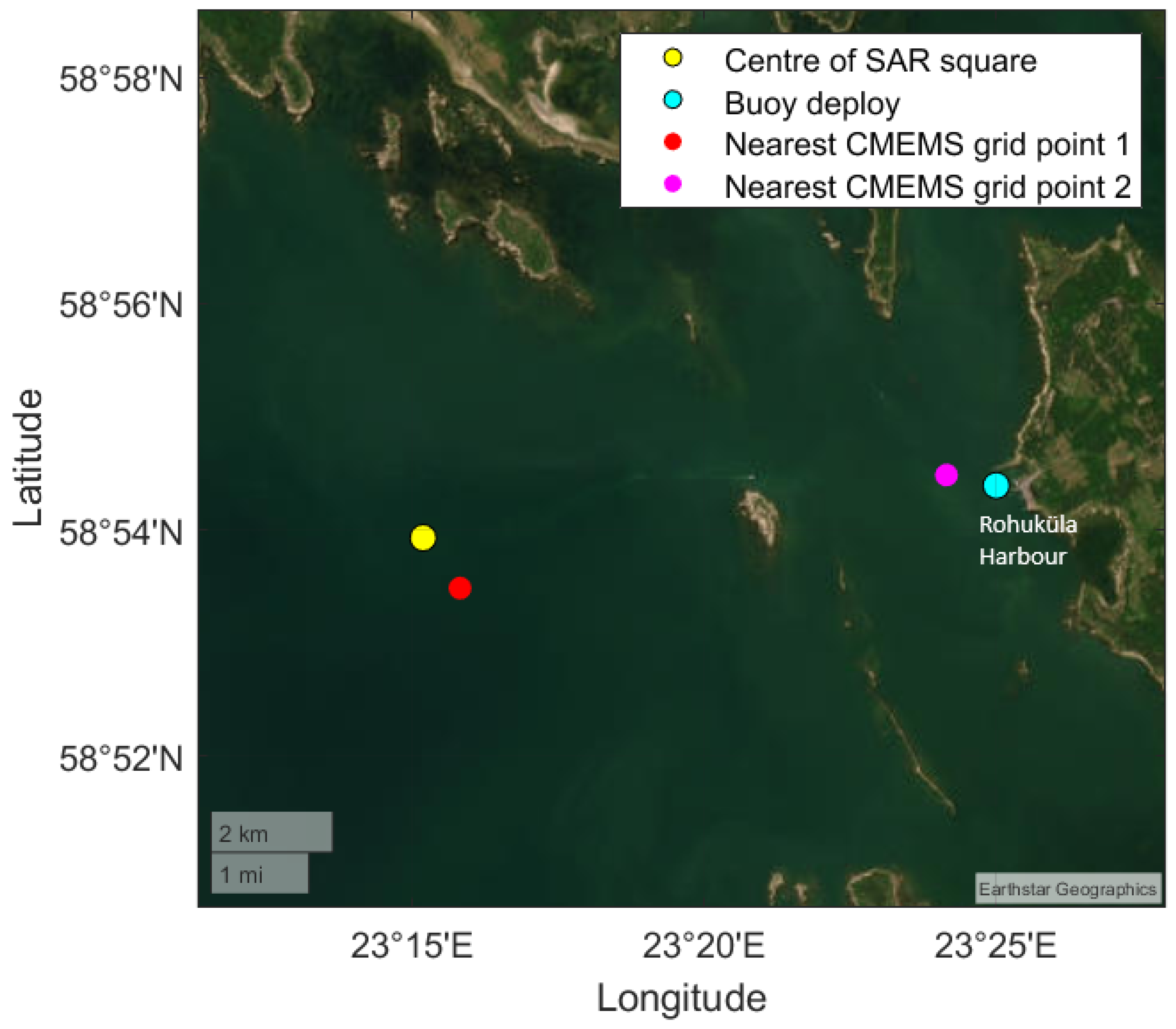
1.2. Study Area and Location Selection

Setting the scene of our analysis, we focused specifically on the territorial waters of Estonia in the Baltic Sea, with the objective of identifying a feasible location for the deployment and validation of wave energy converters (WECs). Our selection process systematically addressed the main development constraints outlined in previous research [9]—namely, limited wave resource intensity, seasonal ice cover, dense maritime traffic, regulatory complexity due to marine protection zones, the absence of open-access resource modeling tools, and sensitivity to public and stakeholder acceptance. Within this national maritime domain, the Väinameri sub-basin emerged as a geographically central and logistically appealing area, yet it is also heavily constrained by environmental regulations. The largest restriction in this region stems from the Natura 2000 network, which designates extensive portions of Väinameri as marine protected areas. However, our detailed spatial assessment revealed that the waters surrounding the port of Rohuküla constitute an important exception—they are located within Väinameri but lie outside of Natura 2000 protection boundaries. This local exemption, combined with the port’s existing infrastructure (mooring, access roads, and cabling), regulatory receptiveness, and proximity to Tallinn—ensuring rapid access for technical maintenance and institutional support—position Rohuküla as a uniquely qualified site for pilot-scale WEC deployment. While the wave energy potential here is moderate, the combination of minimized environmental and logistical constraints makes it one of the few viable nearshore test locations within Estonia’s exclusive maritime jurisdiction. The methodological framework presented in this study is thus not only technically sound but also explicitly adapted to the layered geographic, regulatory, and infrastructural realities of Estonia’s coastal zone (see Figure 1).

In this study, we therefore deployed a smart measurement buoy 100 m seaward of the main pier at Rohuküla harbor. According to our deployment records, the buoy was operational from 20 June 2024 through 8 December 2024 (approximately 172 days) (see Figure 2), allowing us to capture the period of highest wave activity and to recover the instrument just before ice formation in the harbor.

By comparing in situ wave spectra with coincident satellite-derived estimates, we demonstrate how targeted measurements at a single coastal location can support broader spatial assessments. This approach enables site-specific validation while illustrating the potential to extrapolate sparse point observations into reliable regional insights—an essential step toward efficient identification of viable wave energy locations across complex coastal areas.

For the satellite-derived spectra, we selected a grid cell centered approximately 10 km offshore from the buoy deployment site. Because satellite wave products inherently represent spatially aggregated cells rather than point measurements, we carefully delineated the extraction zone to exclude any portion of the shoreline or nearby islands. This precaution ensures that the satellite-derived wave statistics reflect true open-water conditions directly comparable to those recorded by our in situ buoy (see Figure 2).

Figure 2. A detailed description of the study area, near Rohuküla harbor.

Figure 2. A detailed description of the study area, near Rohuküla harbor.

To support the integration of satellite-derived wave spectra into our site-specific wave energy assessment, we selected two reference points within the CMEMS Baltic Sea wave model domain [24]: the location of a high-resolution point observation at the port of Rohuküla, and a manually defined Sentinel-1A SAR subscene. For each, we identified the nearest open-sea CMEMS grid point using geodesic distance. In the case of Rohuküla, we excluded the land-adjacent point and selected the second-nearest ocean-only node to avoid coastal contamination.

2. Materials and Methods

2.1. Measurements Data Preprocessing

Data from satellite missions, together with novel LSTM-based retrieval method (Appendix A) [23], enable wave-climate studies over vastly larger spatial domains than is practical with in situ buoys alone [25]. Because Sentinel-1 SAR and similar sensors have been acquiring data continuously for many years, these long time series make it possible to identify and characterize extreme wave energy peaks—events that are often missed by buoys due to their limited sampling duration and deployment windows (see Figure 3). By filling these temporal gaps, satellite-derived estimates can inform the tuning of wave-energy converters to the true maxima of the sea state, rather than only the more modest heights captured during short buoy deployments, significantly accelerating the acquisition of the required data compared to traditional wave-climate modeling.

Note that the satellite-derived significant wave height curve in Figure 3 does not approach zero. This is not due to frequency-domain filtering but rather a consequence of the training data: all instances with $H_s<0.3$ m were excluded from the supervised learning process to improve model stability. As a result, the model does not predict wave heights below this threshold. Although a low-frequency cutoff at $f_0=0.10$ Hz was applied during spectral preprocessing to suppress noise, its impact on integrated energy is minimal since most wave energy resides at higher frequencies. Conversely, Sentinel-1 SAR backscatter is not sensitive to short gravity waves with frequencies above approximately 0.5 Hz, which are effectively excluded from both training and prediction. The resulting $H_s$ values correspond to the zeroth spectral moment, computed as $H_s\sim 4\sqrt{m_0}=4\sqrt{{\int }_{f_0}^{f_{\max }}S\left(f\right)df}$, and are thus equivalent to the bulk parameter $H_{m0}$ used in in situ validation.

Figure 3. Sentinel-1A SAR and wave-following buoy LainePoiss measurements. Locations correspond to those shown in Figure 2.

Figure 3. Sentinel-1A SAR and wave-following buoy LainePoiss measurements. Locations correspond to those shown in Figure 2.

Measurements are recorded at very different measurement time steps: our wave-following LainePoiss buoy collects 22 min displacement time series at 50 Hz and, after spectral processing, yields a single significant wave height $H_{m0}$ roughly every 22 min on average, whereas Sentinel-1 IW acquisitions occur according to orbital cycles and are further constrained by wind speed, incidence angle and sea-state (in particular, images with $H_s<0.3$ m exhibit only sea clutter and are excluded as low-quality). To make the two records directly comparable, we temporally collocate them by taking each satellite-derived $H_{s\left(\mathrm{sat}\right)}$ timestamp and defining a $\pm 1$ h window around it; within that window we then select the buoy-measured $H_{m0\left(\mathrm{buoy}\right)}$ value whose absolute difference from $H_{s\left(\mathrm{sat}\right)}$ is smallest. These paired values—denoted $H_{s\left(\mathrm{sat}\right)}$ and $H_{m0\left(\mathrm{buoy}\right)}$—form the basis for all subsequent comparisons (see Figure 4).

By contrast, spectrum-to-spectrum comparisons are more nuanced. While our LSTM-predicted wave spectra exhibit strong frequency-to-frequency correlations exceeding 0.8 in the midband range [23] (0.2–0.4 Hz), the root mean square error (RMSE) varies significantly across the spectrum. In the low-frequency band, RMSE is elevated due to the greater natural variability in wave energy. At higher frequencies, however, the RMSE remains low—not because of enhanced model accuracy but rather because the true energy content is minimal and relatively stable. Moreover, the SAR signal saturates near the noise floor in this range, yielding consistently dark image patches that make it easier for the LSTM to infer low spectral energy.

Figure 4. Time-matching of satellite-derived $H_s$ and buoy-measured $H_{m0}$. For the bulk wave heights, our ±1 h pairing yields a Pearson correlation coefficient of r = 0.76 and a root mean square error of RMSE = 0.25 m.

Figure 4. Time-matching of satellite-derived $H_s$ and buoy-measured $H_{m0}$. For the bulk wave heights, our ±1 h pairing yields a Pearson correlation coefficient of r = 0.76 and a root mean square error of RMSE = 0.25 m.

2.2. CMEMS Product Usage

To support the comparative analysis of wave parameters derived from satellite and in situ sources, we incorporated model-based hindcast data from the CMEMS product BALTICSEA_MULTIYEAR_WAV_003_015. This dataset provides a 43+ year time series of hourly wave parameters for the Baltic Sea, generated by the WAve Model (WAM) cycle 4.7. The simulations are forced by ERA5 reanalysis wind fields, with boundary conditions taken from the ERA5 wave reanalysis at Skagerrak. Ice coverage is handled via gridded concentration maps from SMHI and FMI ice services [24].

The dataset includes integrated parameters from the total wave spectrum, including the spectral significant wave height (VHM0) and the spectral moment period VTM10, defined as $T_{\mathrm{m}-1,0}$. These were used to extract modeled wave conditions at the two primary locations of our study: (1) near the in situ deployment site at Rohuküla, and (2) at the central point of a selected Sentinel-1A acquisition subscene. The data enabled temporal and spatial comparisons of modeled wave height and period with corresponding values from satellite and buoy observations, under consistent hourly resolution and nautical-mile scale spatial detail.

The CMEMS hindcast data from BALTICSEA_MULTIYEAR_WAV_003_015 served multiple purposes in this study. First, the model output provided a consistent physical reference for comparing wave parameters such as significant wave height ($H_s$) and mean energy period $T_{\mathrm{m}-1,0}$ with in situ measurements and satellite-derived estimates (see Figure 5 and Figure 6). In total, 43 instances were identified where the wave buoy reported a mean wave period $T_{\mathrm{m}-1,0}$ exceeding 4 s (see Figure 6). In these cases, the significant wave height was dominantly below 1 cm, with only one instance reaching 2 cm. Such events likely represent rare sensor anomalies, potentially caused by sensitivity limitations under low-energy conditions or irregularities in signal processing. Some far-field vessel wake influence could also contribute.

Second, the model data were used to extract time series at two reference points: near the Rohuküla buoy location and the center of a selected Sentinel-1A SAR acquisition subscene. These comparisons allowed us to evaluate cross-platform consistency and assess the representativeness of both observed and modeled wave conditions in the Estonian nearshore environment. Unlike satellite-based products, the CMEMS hindcast fields offer uninterrupted hourly coverage over multiple decades, making them suitable as a climatological baseline.

2.3. Pairing Method for Satellite–Buoy Data Comparison

For initial comparison based on the temporal coverage described above, matched point pairs were created by selecting, for each satellite derived $H_{s\left(\mathrm{sat}\right)}$ timestamp, the nearest buoy-measured value $H_{m0\left(\mathrm{buoy}\right)}$ within a $\pm 1$ h window (i.e., up to one hour before or after the satellite overpass). These temporally collocated pairs—$\left(H_{s\left(\mathrm{sat}\right)},H_{m0\left(\mathrm{buoy}\right)}\right)$—were then plotted to illustrate their agreement (see Figure 7). The ±1 h tolerance was selected as a physically and statistically justified balance. The satellite footprint lies roughly 10–15 km offshore from the LainePoiss buoy, which implies a spatial separation that waves can bridge within one hour under typical group velocities (5–10 m s⁻¹) observed in the Baltic Sea for peak periods of 5–7 s [10]. This time window accommodates natural variability and propagation delays.

2.4. Wave Energy Calculation

To quantify the wave energy resource at both satellite-derived and in situ observation points, we applied a physics-based energy flux formulation appropriate for deep-water conditions. At each time step, the instantaneous wave power per meter of wave crest, $P\left(t\right)$, was computed using the well-established expression

$$P\left(t\right)={\displaystyle \frac{\rho g^2}{64\pi }}{H}_s^2\left(t\right)T_e\left(t\right),$$

(1)

where $\rho$ is the water density (typically in the Baltic Sea 1005–1014 $\mathrm{kg}/{\mathrm{m}}^3$ [26]), g is gravitational acceleration, $H_s\left(t\right)$ is the significant wave height, and $T_e\left(t\right)$ is the energy period. This formulation captures the dependence of wave power on both the height and period of the wave field, assuming a deep-water approximation.

To obtain the total (potential) wave energy resource over the full observation period, we numerically integrated the time series of $P\left(t\right)$ using the trapezoidal rule:

$$E={\int }_{t_0}^{t_1}P\left(t\right)\mathrm{d}t,$$

(2)

yielding energy in joules per meter of wave crest ($\mathrm{J}/\mathrm{m}$). The resulting values were subsequently converted to $\mathrm{MWh}/\mathrm{m}$ for ease of interpretation in an energy system context by dividing by $3.6\times {10}^9$. This methodology enables a consistent and comparable estimation of wave energy input at both satellite and buoy locations, forming the basis for further performance analysis of wave energy converters.

Wave energy flux $P\left(t\right)$ was computed for all three data sources—Sentinel-1 SAR, LainePoiss buoy, and the CMEMS hindcast product. However, the temporal resolution and availability of measurements vary significantly:

CMEMS model: The hindcast product provides wave parameters at regular 1 h intervals, allowing straightforward numerical integration using uniform time steps ($\Delta t=1$ h).

LainePoiss buoy: The buoy produces continuous spectra every 1310 s. Thus, for long-term integration over the full deployment period, a fixed time step of $\Delta t=1310/3600$ h can be assumed.

Sentinel-1 SAR: Satellite acquisitions occur irregularly due to orbital constraints and data filtering (e.g., scenes with $H_s<0.3$ m are excluded). Consequently, $\Delta t$ varies between observations, making it difficult to apply uniform integration. For SAR-based estimates, cumulative energy must be interpreted carefully, often relying on time-weighted averaging or focusing on instantaneous $P\left(t\right)$ values only.

These differences in temporal coverage directly affect the comparability of cumulative energy estimates and must be considered when interpreting energy flux results from mixed observation systems.

3. Results

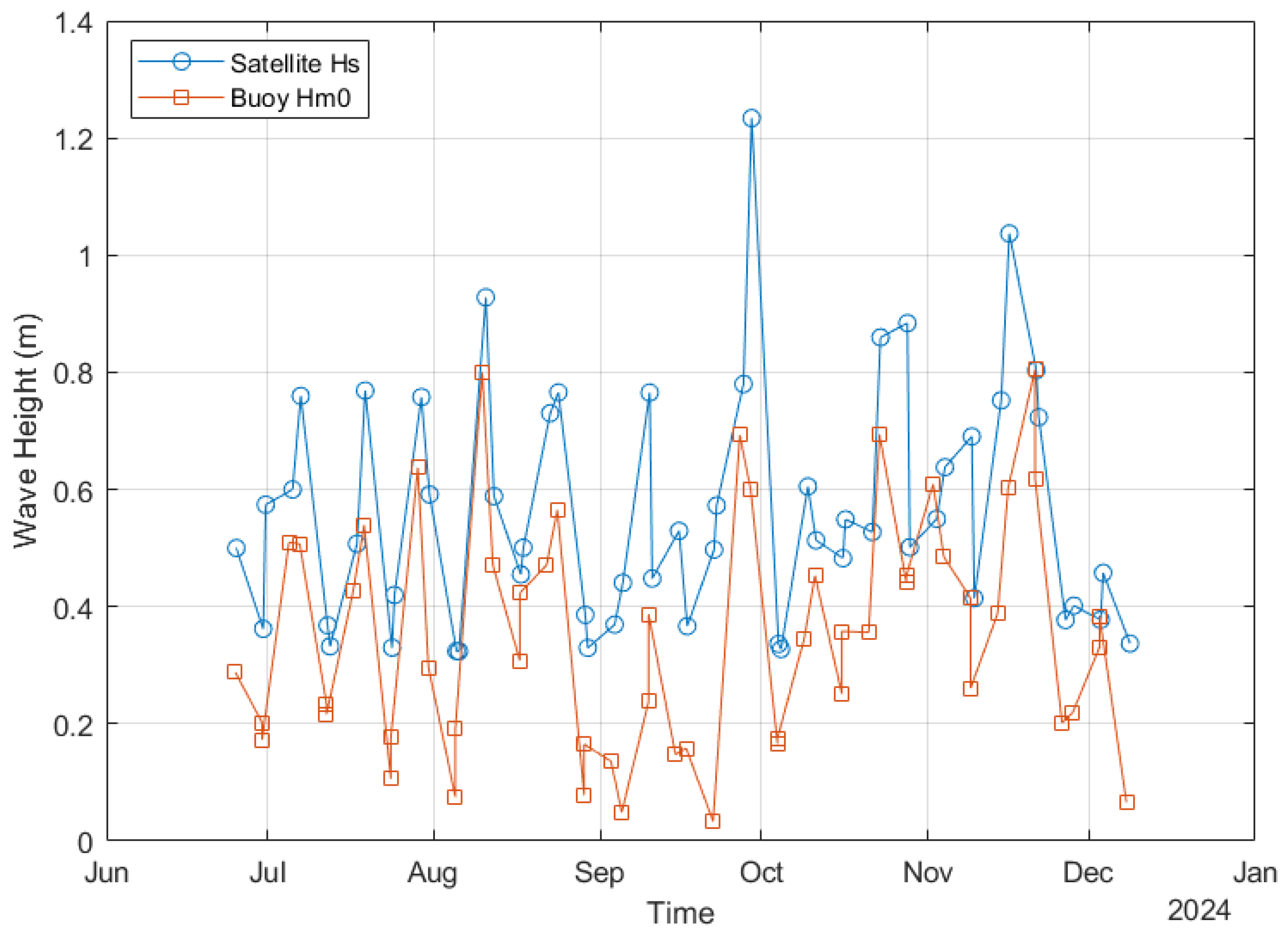
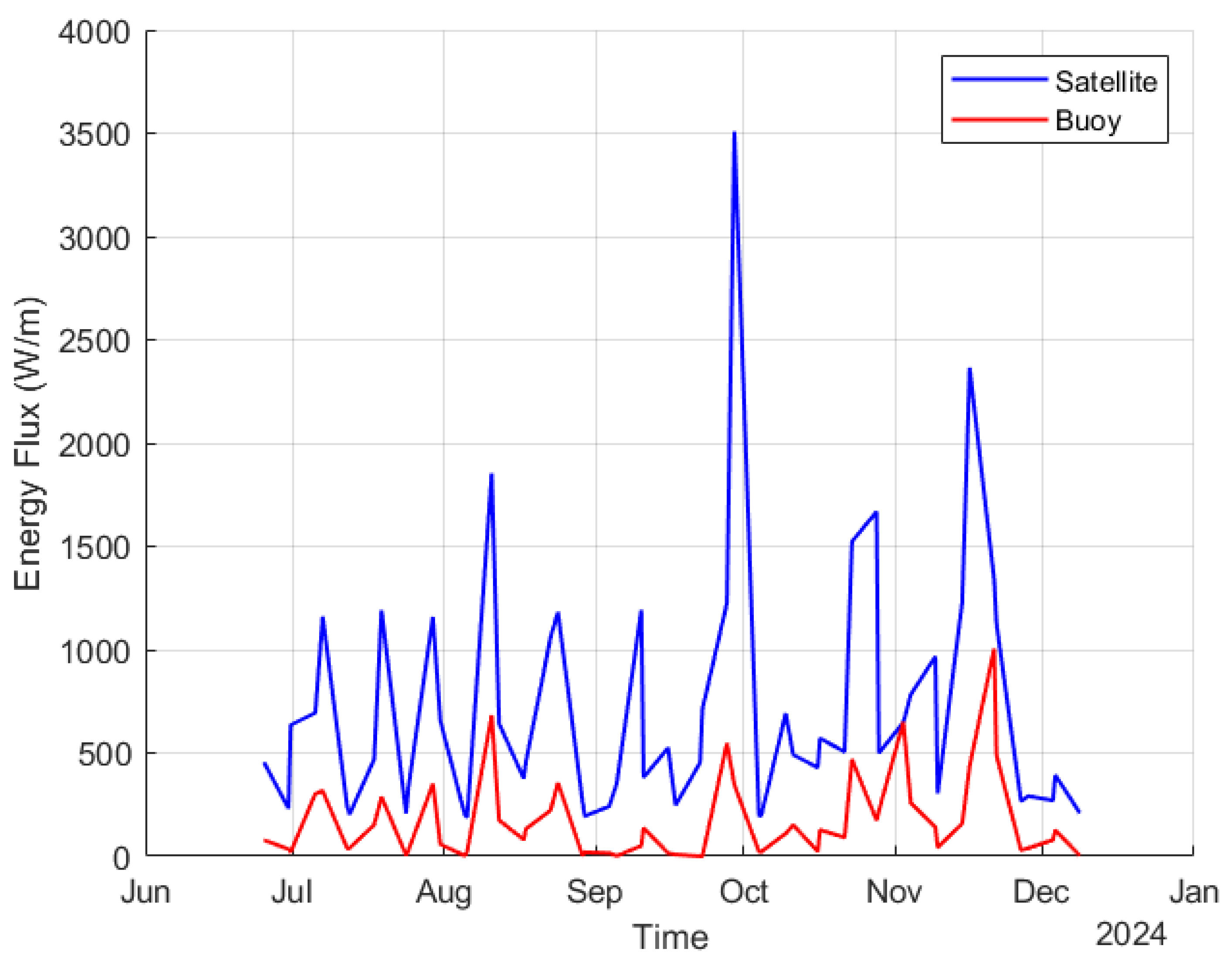
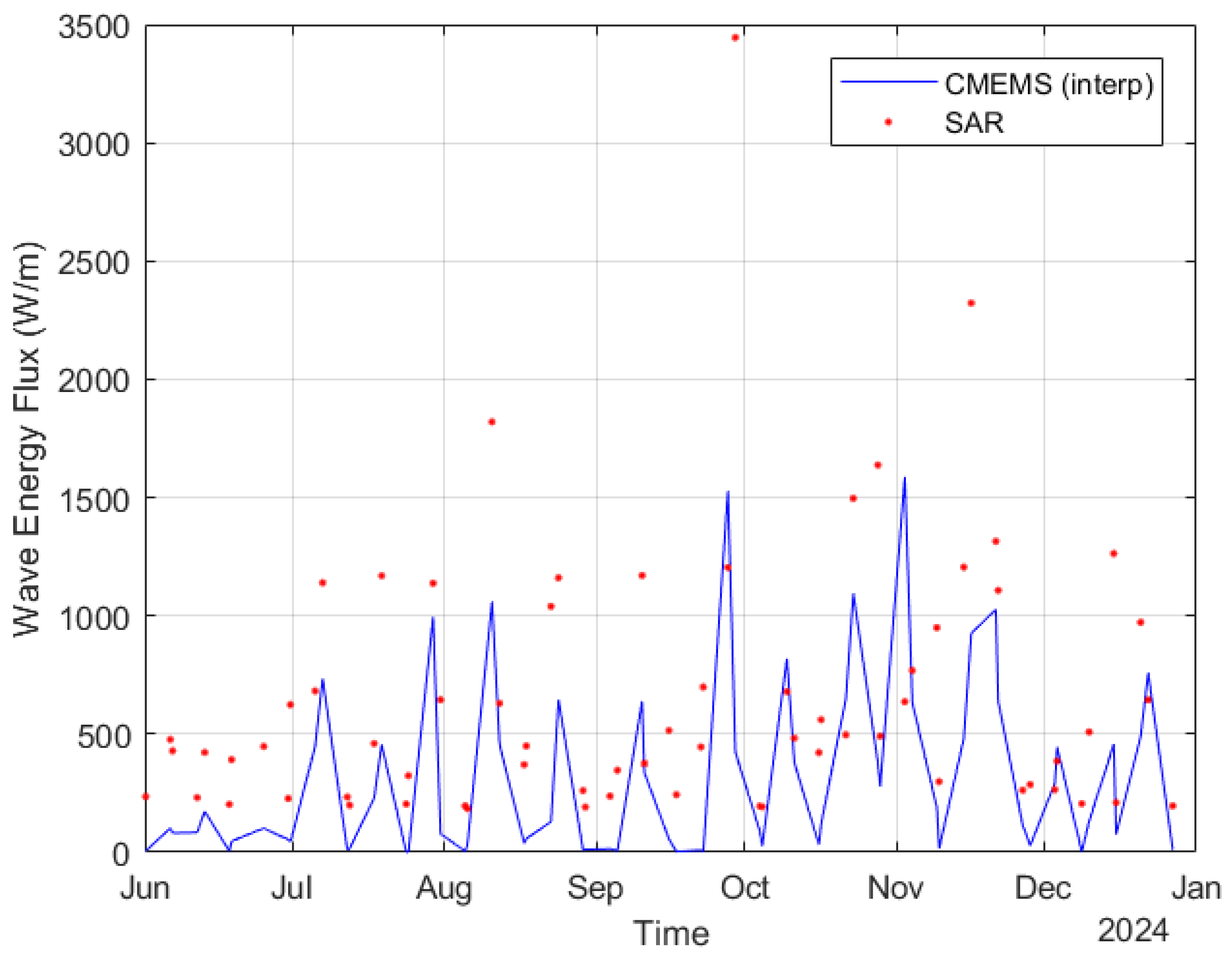
3.1. Wave Energy Conditions

We computed the wave energy resource at both satellite and in situ (“Buoy”) locations by first estimating the instantaneous energy flux per meter of wave crest using the deep-water approximation.

Figure 8 shows the temporal evolution of the wave energy flux $P\left(t\right)$ for both satellite-derived and buoy-derived observations over the full measurement period. For the buoy, only those values falling within a ±1 h window around each satellite acquisition were included, following the pairing approach illustrated in Figure 4 and Figure 7. The maximum instantaneous flux reaches approximately 3508 W/m in the satellite data, while the corresponding mean value is 706 W/m. These values highlight the pronounced differences in energy estimates depending on the data source. The sharp peaks in $P\left(t\right)$ coincide with individual storm events that dominate the seasonal energy input. Due to the irregular temporal sampling of the SAR acquisitions, cumulative energy from satellite data is not reported here. Full buoy and CMEMS statistics, including mean and total energy, are presented in the model–buoy comparison shown in Figure 10.

To evaluate the consistency of the CMEMS hindcast product with other observation sources, we compared the computed wave energy flux (P, in W/m) at two reference locations: (i) the SAR-based satellite acquisition points and (ii) the in situ measurement site at Rohuküla (LainePoiss buoy). Figure 9 shows the interpolated CMEMS fluxes (blue line) versus discrete SAR-derived estimates (red dots), resulting in a root mean square error (RMSE) of 573 W/m, a bias of −344 W/m, and a moderate correlation of 0.58. The substantial underestimation and scatter suggest limited temporal resolution and possible mismatch in the wave period representation in the SAR retrievals.

Figure 8. Time series of instantaneous wave energy flux $P\left(t\right)$ per meter of wave front, comparing satellite-derived (blue) and buoy-derived (red) estimates. The average flux over the analysis period is 706 W/m for the satellite data. Peaks in $P\left(t\right)$ reflect the storm-driven energy injections, while the time series highlight the differing energy capture characteristics of each observation method.

Figure 8. Time series of instantaneous wave energy flux $P\left(t\right)$ per meter of wave front, comparing satellite-derived (blue) and buoy-derived (red) estimates. The average flux over the analysis period is 706 W/m for the satellite data. Peaks in $P\left(t\right)$ reflect the storm-driven energy injections, while the time series highlight the differing energy capture characteristics of each observation method.

Figure 9. Energy flux: SAT together with CMEMS nearest grid point.

Figure 9. Energy flux: SAT together with CMEMS nearest grid point.

In contrast, Figure 10 compares the CMEMS hindcast values at the nearest grid point with hourly in situ buoy observations. The RMSE drops to 119 W/m, the bias is minimal (−41 W/m), and the correlation improves significantly to 0.85. This high agreement indicates that the hindcast model captures the temporal variability of wave energy flux well when compared with ground-truth observations, confirming its value for climatological and resource assessment purposes in the Estonian coastal context. The model data, sampled hourly, yield a mean flux of 78 W/m and a maximum of 799 W/m, corresponding to a total energy resource of 389 kWh/m. In contrast, the buoy data, sampled every 1310 s, exhibit a higher mean flux of 117 W/m and a peak value of 3301 W/m, resulting in a total of 482 kWh/m. These differences highlight both the variability captured by the high-frequency buoy and the broader spatial averaging inherent in the model output.

Unlike satellite-based observations, both the CMEMS model and the buoy dataset provide measurements at regular time intervals, which allows reliable numerical integration of the instantaneous energy flux to obtain cumulative energy estimates.

3.2. Satellite Spectra: LSTM and Sentinel-1

Sentinel-1 SAR imagery was first processed to extract wave number spectra using FFT-based methods. These spatial spectra, representing the distribution of wave energy across wave numbers, served as inputs to a long short-term memory (LSTM) model trained on co-located SAR and NORA3 hindcast spectra. The LSTM effectively learned to approximate the dispersion relation, producing estimated 1D frequency spectra in the range 0.09 to 0.55 Hz. Model inputs included polarization information, imaging geometry, and local bathymetry [23].

Figure 11 shows the 56 Sentinel-1 SAR wave spectra matched in time to the buoy measurements rather than being selected by an arbitrary quality screen. All spectra are plotted on linear axes over the 0.10–0.55 Hz frequency range, and these time-matched satellite spectra form the basis for our LSTM-based spectral reconstruction and comparison.

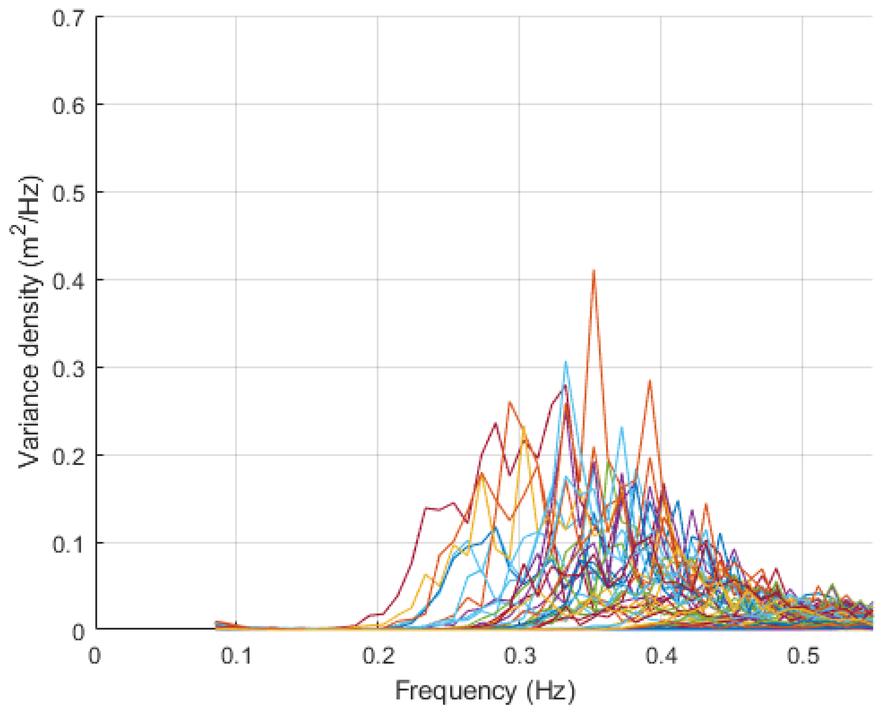
3.3. In Situ Spectra: LainePoiss Buoy

The LainePoiss buoy [22] deployed at Rohuküla harbor recorded continuously vertical and two horizontal accelerations in the Earth reference frame at 50 Hz (pitch, roll and yaw angles were also collected and saved on-board the buoys memory card at 50 Hz). After collecting 65,536 samples, the accelerations were low-pass FIR filtered for anti-aliasing (filter “biting” between 1.5625 Hz and 3.125 Hz) and then downsampled 16 times to yield 4096 data points (ca 22 min) with a sampling frequency of 3.125 Hz. The accelerations were then double integrated in Fourier space in order to reconstruct the vertical displacement time-series (from which, e.g., maximum wave height and other time-series parameters were determined) and to calculate wave variance spectra, from which significant wave height and spectral periods were calculated. The spectra were calculated by bin-averaging 13 neighboring elementary FFT points and tapering with a Hann window. This yielded a spectral resolution of 0.01 Hz; only the frequency range from 0.10 Hz to 0.58 Hz was retained in this study to match the frequency bandwidth of satellite-derived spectra. A total of 59 spectra were selected by matching each Sentinel-1 SAR acquisition to the closest buoy record within a ±1 h window. These time-aligned spectra form the in situ reference set for comparison with LSTM-estimated satellite spectra (see Figure 12).

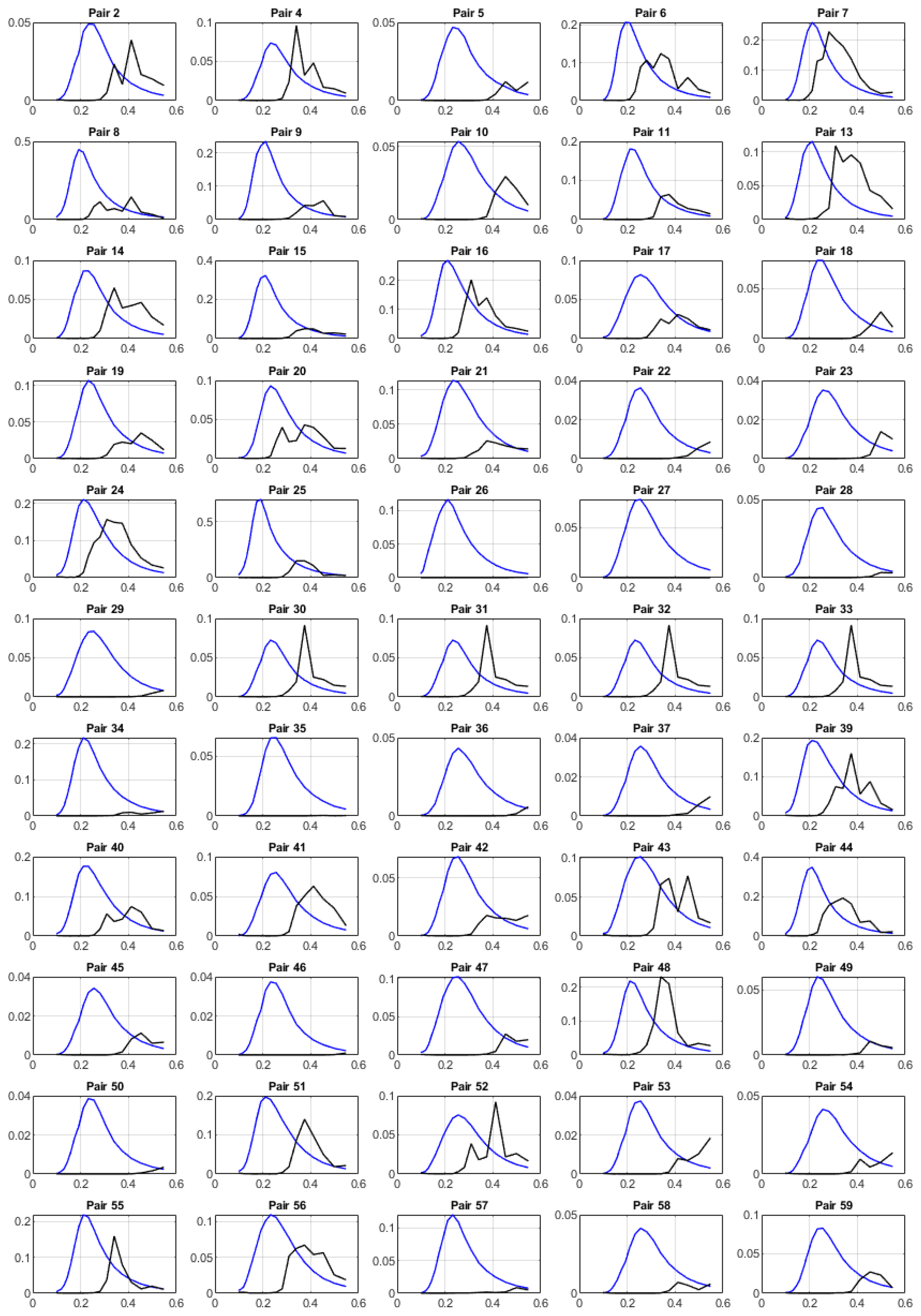
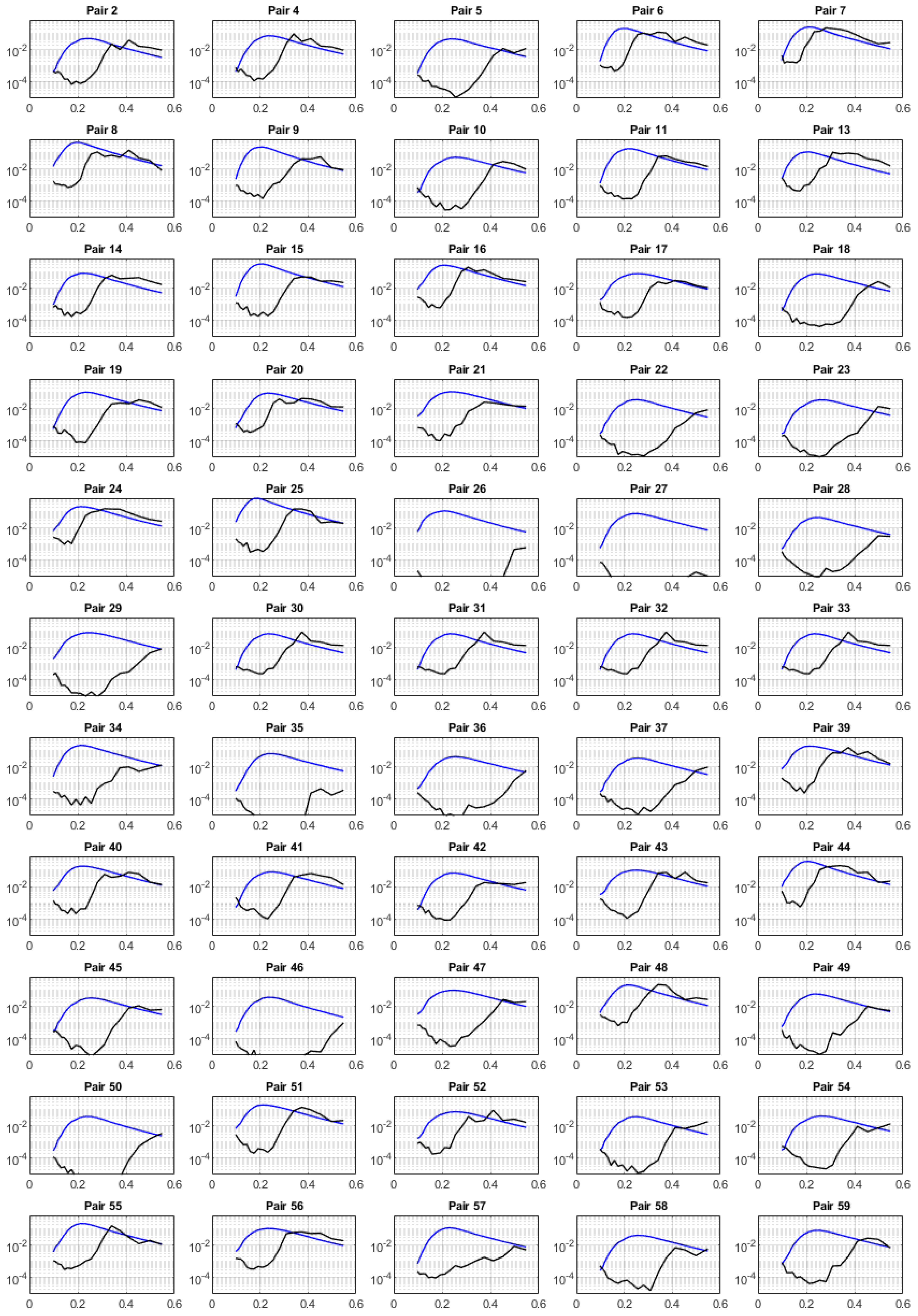
3.4. Spectral Comparison of C-Band SAR and Co-Located In-Situ Measurements

To assess the agreement between co-located spectral estimates, we constructed 56 spectral pairs $\left(S_{\mathrm{sat}}\left(f\right),S_{\mathrm{buoy}}\left(f\right)\right)$ by matching each satellite-derived spectrum to the buoy spectrum closest in time within a $\pm 1$ h window. All spectra were interpolated onto a common frequency grid ranging from 0.10 to 0.55 Hz. The pairwise spectral differences were evaluated using two standard metrics: root mean square error (RMSE) and Pearson correlation coefficient (Corr), both computed over the full frequency band. The resulting mean RMSE was 0.0631 ${\mathrm{m}}^2/\mathrm{Hz}$, and the mean correlation was $-0.25$, reflecting systematic shape discrepancies, particularly in the high-frequency tail. These metrics were aggregated from paired comparisons and are visualized in Figure 13 and Figure 14.

Figure 12. Time-matched buoy-derived wave spectra from the Rohuküla deployment. Colored lines represent different time instances at which buoy data was collocated.

Figure 12. Time-matched buoy-derived wave spectra from the Rohuküla deployment. Colored lines represent different time instances at which buoy data was collocated.

The negative mean correlation indicates a systematic mismatch in spectral shape, particularly in the low-frequency range ($f<0.2\mathrm{Hz}$), where natural variability is high and wave energy is concentrated. Surprisingly, the LSTM model tends to reproduce higher-frequency components ($f>0.4\mathrm{Hz}$) more consistently, despite these lying beyond the effective resolution of Sentinel-1 SAR and being dominated by noise in the raw imagery. While SAR-derived $H_s$ values align reasonably well with buoy measurements (RMSE = 0.25 m, $r=0.76$), the detailed spectral reconstruction remains challenging—highlighting the limitations of current SAR-to-spectrum learning frameworks. To further investigate these discrepancies, we present the same comparisons on logarithmic axes in Figure 14.

To quantify the agreement between C band synthetic aperture radar (SAR) derived wave spectra and co-located point observations (POI), we selected a 512 × 512-pixel subscene centered at 58.898° N, 23.252° E and matched each SAR acquisition to the nearest record in situ in time. All spectra were interpolated onto a common frequency grid and plotted using both linear and logarithmic vertical axes (Figure 13 and Figure 14). For each matched pair, we computed the root mean square error (RMSE) and the Pearson correlation coefficient across the full spectral band. The analysis yielded a mean RMSE of 0.063 ${\mathrm{m}}^2/\mathrm{Hz}$ and a mean correlation of −0.25.

While significant wave height $H_s$ is reproduced with acceptable accuracy, the SAR-based model systematically misestimates energy in the high-frequency tail (periods below approximately 3 s), resulting in poor spectral correlation. This short-period bias is consistent with the known limitations of SAR imaging: a 10 m × 10 m pixel grid (radar resolution 5 m × 20 m) imposes a hard cutoff on the smallest resolvable wavelengths, and nonlinear radar imaging effects further degrade the visibility of small-scale wave “structure”. In addition, the SAR footprint lies several kilometers from the buoy and some scenes exhibit ship-wake contamination, both of which contribute to residual discrepancies.

Figure 13. Pairwise comparison of time-matched wave spectra plotted on linear axes. For each matched pair, the satellite-derived spectrum $S_{\mathrm{sat}}\left(f\right)$ (blue, solid) is compared with the corresponding buoy-derived spectrum $S_{\mathrm{buoy}}\left(f\right)$ (black, solid). The x-axis shows frequency (Hz), and the y-axis represents variance density (${\mathrm{m}}^2/\mathrm{Hz}$). Spectra are plotted in physical units (${\mathrm{m}}^2/\mathrm{Hz}$) over the 0.10–0.55 Hz frequency band.

Figure 13. Pairwise comparison of time-matched wave spectra plotted on linear axes. For each matched pair, the satellite-derived spectrum $S_{\mathrm{sat}}\left(f\right)$ (blue, solid) is compared with the corresponding buoy-derived spectrum $S_{\mathrm{buoy}}\left(f\right)$ (black, solid). The x-axis shows frequency (Hz), and the y-axis represents variance density (${\mathrm{m}}^2/\mathrm{Hz}$). Spectra are plotted in physical units (${\mathrm{m}}^2/\mathrm{Hz}$) over the 0.10–0.55 Hz frequency band.

Figure 14. Pairwise comparison of time-matched wave spectra plotted on logarithmic axes to highlight differences in spectral shape, especially in the high-frequency tail. For each matched pair, the satellite-derived spectrum $S_{\mathrm{sat}}\left(f\right)$ (blue, solid) is compared with the corresponding buoy-derived spectrum $S_{\mathrm{buoy}}\left(f\right)$ (black, solid). The x-axis shows frequency (Hz), and the y-axis represents variance density (${\mathrm{m}}^2/\mathrm{Hz}$). Log-scale representation helps to visualize discrepancies at lower energy levels that are less apparent on linear axes.

Figure 14. Pairwise comparison of time-matched wave spectra plotted on logarithmic axes to highlight differences in spectral shape, especially in the high-frequency tail. For each matched pair, the satellite-derived spectrum $S_{\mathrm{sat}}\left(f\right)$ (blue, solid) is compared with the corresponding buoy-derived spectrum $S_{\mathrm{buoy}}\left(f\right)$ (black, solid). The x-axis shows frequency (Hz), and the y-axis represents variance density (${\mathrm{m}}^2/\mathrm{Hz}$). Log-scale representation helps to visualize discrepancies at lower energy levels that are less apparent on linear axes.

4. Discussion

4.1. Wave Energy Hotspot Definition and Site Evaluation

Drawing on the hotspot criteria of Soomere and Eelsalu (2014) and Kovaleva et al. (2017), we refine the definition for our semi-sheltered archipelago setting: a wave energy hotspot is any contiguous coastal segment of at least 5 km over which the long-term onshore-directed mean flux exceeds 1 kW m⁻¹ [10,11]. Our experimental site, centered at 58.907° N, 23.417° E within the Estonian archipelago, experiences fetch-limited, island-filtered wave climates. Applying the deep-water approximation to regularly sampled in situ and model data over July–December 2024 yields a cumulative energy of 482 kWh m⁻¹ for the buoy and 389 kWh m⁻¹ for the CMEMS hindcast, corresponding to mean onshore fluxes of 117 and 78 W m⁻¹, respectively. Both values fall below the 1 kW m⁻¹ hotspot threshold, confirming that the site does not qualify as a wave energy hotspot, though the flux remains sufficient for pilot-scale converter trials in protected Baltic waters. For reference, the mean flux derived from satellite observations over the same period is 706 W m⁻¹ but cumulative energy is not reported due to irregular temporal sampling.

Despite not meeting the 1 kW m⁻¹ threshold for classification as a wave energy hotspot, the Rohuküla archipelago site presents several features that make it well suited for the controlled testing of wave energy converters. First, the presence of a modest but persistent background energy level—evidenced by the buoy-derived mean flux of 0.15 kW m⁻¹ sustained over months—ensures regular forcing conditions that are sufficient for power take-off activation without subjecting the device to destructive loads. This mitigates early-stage deployment risks and supports continuous endurance testing. Second, the site occasionally experiences pronounced short-term surges in wave energy flux during storm events.

The buoy record shows peak onshore flux values reaching approximately 3300 W/m (Figure 10), while satellite-derived fluxes attain maxima of around 3508 W/m (Figure 8).

These storm-driven extremes offer real-world conditions for stress testing converter durability, even though the site’s long-term average remains below classical hotspot levels. These intermittent peaks simulate exposure to more energetic open-sea conditions, enabling the assessment of structural resilience and adaptive control strategies. Lastly, the semi-sheltered, island-filtered environment provides natural protection and logistical accessibility, which are essential for iterative design, monitoring, and retrieval. Altogether, this hybrid regime—low average flux punctuated by storm-driven surges—offers a unique real-world testbed for Baltic-optimized WEC development.

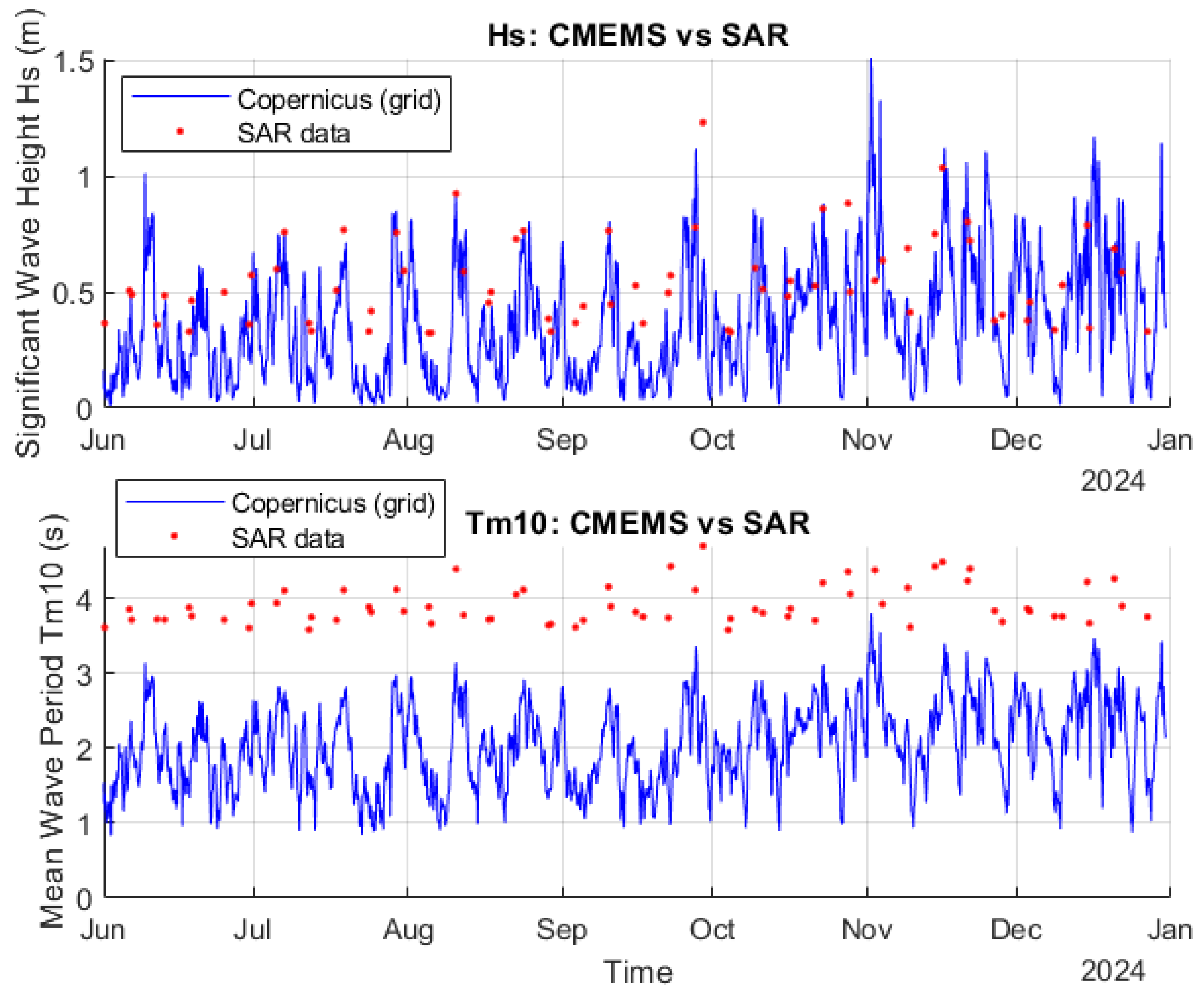
4.2. Satellite Derived Approach Validation and Key Limitation for Wave Energy Flux Prediction

The high fidelity of the satellite-derived spectra validates the LSTM model’s use in the Baltic. Key limitations include the inability to detect ultra-calm states and under-representation of short local waves in the training dataset. Nonetheless, the model offers a valuable tool for large-scale resource mapping. Our spectral comparisons between the satellite-based LSTM retrievals and in situ buoy measurements clearly indicate that, despite accurate predictions of bulk wave parameters such as significant wave height, SAR-based reconstructions face intrinsic limitations in resolving detailed spectral structures at short periods. These discrepancies primarily arise from fundamental SAR imaging constraints: the pixel resolution (10 × 10 m pixel, effectively 5 × 20 m radar resolution) sets a physical limit on detectable wavelengths, which inherently excludes the accurate characterization of high-frequency (short-period) wave fields. Furthermore, nonlinear radar backscatter effects further attenuate spectral fidelity at these scales, a phenomenon accentuated in sheltered environments like the Väinameri archipelago, where wave energy predominantly manifests as locally generated, high-frequency seas rather than clearly structured swell. Additionally, proximity to shipping routes introduces localized disturbances, further diminishing spectral accuracy. Recognizing these constraints, future SAR-based wave studies in the Baltic Sea should strategically target locations characterized by more developed, longer-period waves—such as open coastal stretches near Kõpu or Vilsandi—thus maximizing the inherent strengths of radar imaging techniques and providing a more robust dataset for model refinement.

4.3. Uncertainties, Limitations, and Future Directions

In this study, we have addressed several key uncertainties and limitations associated with deploying wave energy converters (WECs) in the Baltic Sea, many of which were initially outlined in earlier sections. Our assessment included an evaluation of wave resource variability, site-specific conditions, and operational constraints using a combination of CMEMS model hindcasts, Sentinel-1 SAR imagery enhanced by deep learning techniques, and precise in situ measurements obtained from a wave-following LainePoiss buoy [22].

The present findings align with and expand upon previous studies, such as Vidjajev et al. (2022) [9], which highlighted the key environmental, economic, and political constraints in the Baltic Sea region. These include limited wave resource intensity, seasonal ice coverage, dense maritime traffic, and complex regulatory frameworks due to the Natura 2000 protected areas network. The prior assessment underscores the significant differences between open-ocean environments, where devices such as the Pelamis WEC analyzed by Alireza Vakili et al. (2025) [27] operate effectively, and the more restricted wave climates characteristic of semi-enclosed seas like the Baltic Sea.

Indeed, open-ocean conditions provide a more consistent and higher-intensity wave energy resource, facilitating the operation of large-scale, high-capacity converters such as Pelamis. In contrast, the Baltic Sea, particularly regions such as Väinameri, features markedly lower wave heights and periods, substantially restricting the applicability of such large-scale converters. Consequently, the primary challenge in semi-enclosed seas lies not in optimizing energy capture but in identifying suitable locations that balance wave availability with minimal environmental and infrastructural constraints. This encompasses considerations such as proximity to existing infrastructure, the avoidance of protected areas, and the careful management of marine traffic.

One aspect that warrants further attention is the quantification of uncertainty in wave energy estimates derived from these different sources. While this study focused on establishing the methodological framework and demonstrating cross-validation potential, it did not formally assess the statistical uncertainty associated with the results. Given the observed variability between in situ, satellite, and model data, we recognize that incorporating such analysis is important for enhancing the reliability of energy planning and investment decisions. Future studies should thus aim to implement uncertainty quantification protocols to capture the range and confidence levels of derived wave energy values.

Infrastructural proximity is a critical factor highlighted by multiple studies and our current research. Although measurement buoys represent one of the most accurate tools for assessing local wave resources, their deployment is time-consuming, costly, and spatially limited. Consequently, the Baltic Sea region, with its numerous islands and intricate coastline, requires innovative alternatives capable of rapidly and extensively mapping wave resources over large areas. Historically, mathematical models have fulfilled this role; however, their accuracy can be challenged by complex coastlines and the presence of islands, as these conditions demand extensive calibration and validation periods. Our research, therefore, points toward satellite-based methods, particularly SAR imagery enhanced by machine learning models such as long short-term memory (LSTM) neural networks as highly promising for overcoming these limitations. The capability of SAR-derived spectra, combined with precise buoy measurements, represents a significant advancement, facilitating rapid and spatially extensive resource assessments. Future research directions should thus prioritize refining these satellite-based methodologies, improving their resolution, and integrating them into accessible, open-source tools to facilitate stakeholder decision-making.

This integrated approach—combining in situ measurements, advanced satellite retrieval techniques, and numerical models—offers the most feasible path forward. Developing user-friendly platforms that provide accurate, real-time assessments of wave energy potential can significantly accelerate the identification and development of optimal WEC deployment sites, particularly in complex environments like Väinameri. Future studies should also explore deeper cross-disciplinary collaborations, engaging stakeholders across regulatory, economic, and environmental sectors to comprehensively address these intertwined constraints.

5. Conclusions

Taken together, these findings highlight both the promise and current limitations of SAR-based wave spectral estimation in the Baltic Sea. Our results show that while C-band Sentinel-1 SAR imagery—when processed through a long short-term memory (LSTM) neural network—can robustly estimate integrated bulk wave parameters such as significant wave height ($H_s$), it faces greater challenges in reconstructing the full spectral shape, particularly in the low-frequency range where energy is concentrated and natural variability is high. In contrast, higher-frequency components are often estimated with surprising consistency, despite lying beyond the nominal sensitivity of SAR, likely due to their relatively stable and low-energy nature.

The trained LSTM model, based on over 71,000 co-located Sentinel-1 and hindcast spectra, achieved a mean $H_s$ RMSE of 0.39 m and frequency-to-frequency correlations exceeding 0.8 in the 0.2–0.4 Hz range. These performance levels are competitive with state-of-the-art empirical methods.

However, the SAR-based approach remains constrained by several factors intrinsic to both the radar imaging process and the semi-sheltered nature of the Baltic Sea. The effective resolution of SAR imagery limits the reliable detection of short-period waves with frequencies above 0.15 Hz, where the image spectra are increasingly dominated by noise. Additionally, nonlinear backscatter effects, frequent land interference, and the limited visibility of short-crested seas introduce systematic uncertainty in spectral reconstruction. Despite these limitations, the LSTM model outperforms traditional analytical inversion schemes, particularly under wind–sea-dominated conditions where directional swell components are absent.

Regarding practical deployment, our study underscores that while the Väinameri region—including our test site near Rohuküla—does not satisfy the classical wave energy hotspot threshold of 1 kW m⁻¹ in mean onshore flux, it remains well suited for pilot-scale wave energy converter (WEC) testing. The buoy-measured mean flux of 117 W m⁻¹ provides a steady background energy level suitable for endurance testing, while intermittent storm surges—reaching up to 3300 W m⁻¹—enable structural load validation. This hybrid regime of persistent low energy punctuated by short-duration peaks offers an ideal setting for developing WECs tailored to the constraints of the Baltic environment. Logistical accessibility, natural shelter, and fetch-limited wave climates further support the suitability of such test sites.

From a methodological standpoint, three classes of spectral estimation were evaluated: analytical transfer-function-based inversion, empirical bulk parameter regression, and LSTM-based learning from image spectra. Among these, the LSTM-based method proved to be the most robust across sea states, although its accuracy declined for wave periods below 3 s. Future improvements should aim at expanding training datasets with high-resolution in situ spectra during extreme conditions, incorporating directional information more effectively, and applying hybrid models that combine satellite and model data sources.

We recommend that future validation campaigns prioritize more open coastal sites—such as the Kõpu or Vilsandi peninsula regions—where longer-period wave systems dominate and SAR imaging performs more consistently. Ultimately, this study demonstrates that hybrid SAR–buoy approaches, powered by deep learning, can serve as scalable and transferable tools for spectral wave characterization across spatially complex and data-sparse marine domains like the Baltic Sea. These techniques hold promise not only for resource mapping but also for the siting, risk assessment, and adaptive operation of next-generation wave energy technologies.

References

1. Eurostat. Renewable Energy Statistics. 2025. Available online: https://ec.europa.eu/eurostat/statistics-explained/index.php?title=Renewable_energy_statistics (accessed on 1 March 2025).
2. Robins, P.E.; Neill, S.P.; Lewis, M.J.; Ward, S.L. Characterising the spatial and temporal variability of the tidal-stream energy resource over the northwest European shelf seas. Appl. Energy 2015, 147, 510–522. [Google Scholar] [CrossRef]
3. Clément, A.; McCullen, P.; Falcão, A.; Fiorentino, A.; Gardner, F.; Hammarlund, K.; Lemonis, G.; Lewis, T.; Nielsen, K.; Petroncini, S.; et al. Wave energy in Europe: Current status and perspectives. Renew. Sustain. Energy Rev. 2002, 6, 405–431. [Google Scholar] [CrossRef]
4. Lebedeva, K.; Borodinecs, A.; Palcikovskis, A.; Wawerka, R.; Skandalos, N. Estimation of LCOE for PV electricity production in the Baltic States—Latvia, Lithuania and Estonia until 2050. Renew. Sustain. Energy Transit. 2025, 7, 100110. [Google Scholar] [CrossRef]
5. Augutis, J.; Krikštolaitis, R.; Martišauskas, L.; Urbonienė, S.; Urbonas, R.; Ušpurienė, A.B. Analysis of energy security level in the Baltic States based on indicator approach. Energy 2020, 199, 117427. [Google Scholar] [CrossRef]
6. Fang, S.; Jaffe, A.M.; Loch-Temzelides, T.; Lo Prete, C. Electricity grids and geopolitics: A game-theoretic analysis of the synchronization of the Baltic States’ electricity networks with Continental Europe. Energy Policy 2024, 188, 114068. [Google Scholar] [CrossRef]
7. Laktuka, K.; Pakere, I.; Kalnbalkite, A.; Zlaugotne, B.; Blumberga, D. Renewable energy project implementation: Will the Baltic States catch up with the Nordic countries? Util. Policy 2023, 82, 101577. [Google Scholar] [CrossRef]
8. Saha, P.; Kar, A.; Behera, R.R.; Pandey, A.; Chandrasekhar, P.; Kumar, A. Performance optimization of hybrid renewable energy system for small scale micro-grid. Mater. Today Proc. 2022, 63, 527–534. [Google Scholar] [CrossRef]
9. Vidjajev, N.; Palu, R.; Terentjev, J.; Hilmola, O.P.; Alari, V. Assessment of the Development Limitations for Wave Energy Utilization in the Baltic Sea. Sustainability 2022, 14, 2832. [Google Scholar] [CrossRef]
10. Soomere, T.; Eelsalu, M. On the wave energy potential along the eastern Baltic Sea coast. Renew. Energy 2014, 71, 221–233. [Google Scholar] [CrossRef]
11. Kovaleva, O.; Eelsalu, M.; Soomere, T. Hot-spots of large wave energy resources in relatively sheltered sections of the Baltic Sea coast. Renew. Sustain. Energy Rev. 2017, 74, 424–437. [Google Scholar] [CrossRef]
12. Sokolov, A.; Chubarenko, B. Baltic sea wave climate in 1979–2018: Numerical modelling results. Ocean Eng. 2024, 297, 117088. [Google Scholar] [CrossRef]
13. Björkqvist, J.V.; Lukas, I.; Alari, V.; van Vledder, G.P.; Hulst, S.; Pettersson, H.; Behrens, A.; Männik, A. Comparing a 41-year model hindcast with decades of wave measurements from the Baltic Sea. Ocean Eng. 2018, 152, 57–71. [Google Scholar] [CrossRef]
14. Samlas, O.; Luik, S.T.; Korabel, V.; She, J.; Lips, U. Applicability of Copernicus marine service products for the eutrophication status assessment of the Baltic Sea. Mar. Pollut. Bull. 2025, 216, 117975. [Google Scholar] [CrossRef] [PubMed]
15. Pleskachevsky, A.; Tings, B.; Wiehle, S.; Imber, J.; Jacobsen, S. Multiparametric sea state fields from synthetic aperture radar for maritime situational awareness. Remote Sens. Environ. 2022, 280, 113200. [Google Scholar] [CrossRef]
16. Alday, M.; Lavidas, G. The ECHOWAVE Hindcast: A 30-years high resolution database for wave energy applications in North Atlantic European waters. Renew. Energy 2024, 236, 121391. [Google Scholar] [CrossRef]
17. Scala, P.; Manno, G.; Ingrassia, E.; Ciraolo, G. Combining Conv-LSTM and wind-wave data for enhanced sea wave forecasting in the Mediterranean Sea. Ocean Eng. 2025, 326, 120917. [Google Scholar] [CrossRef]
18. Leng, S.; Shao, W.; Nunziata, F.; Migliaccio, M. An Algorithm for One-dimensional Wave Spectrum Retrieval from Gaofen-3 by Deep Learning. J. Atmos. Ocean. Technol. 2025, 42, 621–636. [Google Scholar] [CrossRef]
19. Wu, K.; Li, X.M. Deep learning for retrieving omni-directional ocean wave spectra from spaceborne synthetic aperture radar. Remote Sens. Environ. 2024, 314, 114386. [Google Scholar] [CrossRef]
20. Daniljuk, M.; Lastovko, I.; Rikka, S.; Nõmm, S. Statistical Machine Learning Techniques for Wave Spectre Estimation in Coastal Seas. In Recent Challenges in Intelligent Information and Database Systems, Proceedings of the 17th Asian Conference, ACIIDS 2025, Kitakyushu, Japan, 23–25 April 2025; Springer Nature: Singapore, 2025. [Google Scholar] [CrossRef]
21. Tripathi, S.; Chapron, B.; Collard, F.; Guitton, G.; Lopez-Radcenco, M.; Mouche, A.; Fablet, R. Deep Learning Inversion of Ocean Wave Spectrum from SAR Satellite Observations. In Proceedings of the ICASSP 2024—2024 IEEE International Conference on Acoustics, Speech and Signal Processing (ICASSP), Seoul, Republic of Korea, 14–19 April 2024; pp. 8711–8715. [Google Scholar] [CrossRef]
22. Alari, V.; Björkqvist, J.V.; Kaldvee, V.; Mölder, K.; Rikka, S.; Kask-Korb, A.; Vahter, K.; Pärt, S.; Vidjajev, N.; Tõnisson, H. LainePoiss(R)—A Lightweight and Ice-Resistant Wave Buoy. J. Atmos. Ocean. Technol. 2022, 39, 573–594. [Google Scholar] [CrossRef]
23. Rikka, S.; Nõmm, S.; Alari, V.; Simon, M.; Björkqvist, J.V. Wave Density Spectra Estimation with LSTM from Sentinel-1 SAR in the Baltic Sea. In Proceedings of the IEEE/OES Thirteenth Current, Waves and Turbulence Measurement (CWTM), Wanchese, NC, USA, 18–20 March 2024; pp. 1–5. [Google Scholar] [CrossRef]
24. E.U. Copernicus Marine Service Information (CMEMS). Marine Data Store (MDS); In Baltic Sea Wave Hindcast; Finnish Meteorological Institute (FMI): Helsinki, Finland, 2025. [Google Scholar] [CrossRef]
25. O’Connell, R.; de Montera, L.; Peters, J.L.; Horion, S. An updated assessment of Ireland’s wave energy resource using satellite data assimilation and a revised wave period ratio. Renew. Energy 2020, 160, 1431–1444. [Google Scholar] [CrossRef]
26. Leppäranta, M.; Myrberg, K. Physical Oceanography of the Baltic Sea, 1st ed.; Springer Praxis Books; Springer: Berlin/Heidelberg, Germany, 2009; 378p. [Google Scholar] [CrossRef]
27. Vakili, A.; Pourzangbar, A.; Ettefagh, M.M.; Abdollahi Haghghi, M. Optimal control strategy for enhancing energy efficiency of Pelamis wave energy converter: A Simulink-based simulation approach. Renew. Energy Focus 2025, 53, 100685. [Google Scholar] [CrossRef]
28. Pleskachevsky, A.; Jacobsen, S.; Tings, B.; Schwarz, E. Estimation of sea state from Sentinel-1 Synthetic aperture radar imagery for maritime situation awareness. Int. J. Remote Sens. 2019, 40, 4104–4142. [Google Scholar] [CrossRef]
29. Li, X.M.; Huang, B. A global sea state dataset from spaceborne synthetic aperture radar wave mode data. Sci. Data 2020, 7, 261. [Google Scholar] [CrossRef] [PubMed]
Figure 1. Test site location in Europe: The left panel shows the broader Baltic Sea region, with the test area located in Estonian territorial waters (magenta marker), in the Väinameri sub-basin between the mainland and Hiiumaa island. The right panel provides a close-up of the site near Rohuküla harbor (cyan marker).
Energies 18 03843 g001
Figure 5. Significant wave height and wave mean period comparison from SAR and nearest CMEMS grid point.
Energies 18 03843 g005
Figure 6. Significant wave height and wave mean period comparison from Rohuküla buoy and nearest CMEMS grid point.
Energies 18 03843 g006
Figure 7. Temporally collocated pairs of satellite-derived significant wave heights H s ( sat ) and in situ buoy measurements H m 0 ( buoy ) . Each pair was matched by selecting, for every Sentinel-1 overpass, the closest available buoy value within a ± 1 h time window.
Energies 18 03843 g007
Figure 10. Instantaneous wave energy flux P ( t ) per meter of wave front from CMEMS (blue) and buoy (green) data over the full overlapping period. The average flux is 78 W/m for CMEMS and 117 W/m for the buoy, with respective totals of 389 and 482 kWh/m.
Energies 18 03843 g010
Figure 11. Time-matched Sentinel-1 SAR spectra used for LSTM-based spectral comparison. A total of 56 spectra were extracted from SAR acquisitions and paired with in situ buoy measurements within a ±1 h window. Each spectrum represents a 1D frequency distribution estimated via an LSTM model trained on co-located SAR and NORA3 wave spectra. Colored lines represent different time instances at which satellite data was collocated.
Energies 18 03843 g011
Disclaimer/Publisher’s Note: The statements, opinions and data contained in all publications are solely those of the individual author(s) and contributor(s) and not of MDPI and/or the editor(s). MDPI and/or the editor(s) disclaim responsibility for any injury to people or property resulting from any ideas, methods, instructions or products referred to in the content.