A Novel Back Propagation Neural Network Based on the Harris Hawks Optimization Algorithm for the Remaining Useful Life Prediction of Lithium-Ion Batteries

Abstract

Remaining useful life (RUL) serves as a pivotal metric for quantifying lithium-ion batteries’ state of health (SOH) in electric vehicles and plays a crucial role in ensuring their safety and reliability. In order to achieve accurate and reliable RUL prediction, a novel RUL prediction method which employs a back propagation (BP) neural network based on the Harris Hawks optimization (HHO) algorithm is proposed. This method optimizes the BP parameters using the improved HHO algorithm. At first, the circle chaotic mapping method is utilized to solve the problem of the initial value. Considering the problem of local convergence, Gaussian mutation is introduced to improve the search ability of the algorithm. Subsequently, two key health factors are selected as input features for the model, including the constant-current charging isovoltage rise time and constant-current discharging isovoltage drop time. The model is validated using aging data from commercial lithium iron phosphate (LiFePO₄) batteries. Finally, the model is thoroughly verified under an aging test. Experimental validation using training sets comprising 50%, 60%, and 70% of the cycle data demonstrates superior predictive performance, with mean absolute error (MAE) values below 0.012, root mean square error (RMSE) values below 0.017 and mean absolute percentage error (MAPE) within 0.95%. The results indicate that the model significantly improves prediction accuracy, robustness and searchability.

1. Introduction

Given the prominence of global energy crisis and growing concern for environmental issues, new energy vehicles, especially electric vehicles (EVs), are expected to replace traditional fuel vehicles to mitigate carbon emissions [1,2]. Lithium-ion batteries (LIBs), serving as the core energy storage component in EVs, have been widely utilized due to their high energy density, extended cycle life and low self-discharge rate [3]. However, as the number of operational cycles increases, LIBs inevitably undergo the aging process, resulting in a decline in available battery capacity and safety [4]. Therefore, accurate monitoring and estimation of battery state of health (SOH) are critical to maintaining the operational efficiency and reliability of EVs. Furthermore, evaluating the remaining useful life (RUL) of LIBs can effectively resolve battery recycling and secondary utilization problems. Such evaluations hold significant economic, resource conservation, and environmental protection value [5].

The methods for estimating SOH and predicting RUL of LIBs can be mainly classified into model-based and data-driven approaches [6,7]. The model-based method analyzes the inner relationship between battery capacity and cycle count by establishing accurate models, including an electrochemical model and an equivalent circuit model [8,9]. For instance, Bian et al. combined the open-circuit voltage model and incremental capacity analysis to estimate the SOH, under significant temperature changes, the method has high estimation accuracy [10]. Bartlett et al. also proposed a reduced-order electrochemical model based on the single-particle model (SPM), enhancing the model accuracy by incorporating liquid-phase diffusion dynamics into the traditional SPM [11]. While these model-based methods effectively demonstrate the physical and electrochemical characteristic of batteries, they are unable to deal with the complexity of internal principles and uncertainty of external operating conditions [12]. In contrast, the data-driven method, as a black-box algorithm, can extract health factors from charging and discharging data by training. Establishing mathematical relationship between input features and available battery capacity allows for the investigation of interactions between external parameters and internal states, thus eliminating the necessity of developing complex battery models. The continuous experimental data is used as the time sequence to describe the principles of data sequence, which can evaluate the SOH and is more applicable for online estimation [13]. Common data-driven methods mainly include statistical model, machine learning model, and deep learning model [14,15]. Feng et al. proposed a novel SOH evaluation model with an error compensation mechanism by integrating an autoregressive model, discharge time during the same voltage range, and a relevance vector machine model for LIBs with long cycles [16]. Chen et al. introduced a fusion model based on the autoregressive moving average (ARMA) model and the Elman neural network [17]. RUL prediction using statistical models is generally easy to understand and implement. However, it often assumes that the data follows a specific distribution, which can lead to poor performance when addressing nonlinear problems. Patil et al. developed a type of RUL prediction method based on support vector machine (SVM) learning, which involves extracting features from data such as voltage, current, and temperature curves for training, and performing real-time estimation of RUL [18]. Xue et al. utilized segmented charging voltage input into the relevance vector machine for RUL prediction, analyzing 21 voltage feature segments (VFS) of various voltage ranges to assess the impact of each voltage interval on capacity prediction [19]. Machine learning-based RUL prediction can accurately predict and monitor battery status using a large amount of historical battery data and real-time collected data, and it can quickly perform fault diagnosis and maintenance. Nonetheless, it requires a substantial amount of data to train the model, consuming considerable computational resources and time. Moreover, the model is prone to overfitting or underfitting issues. In recent years, deep learning methods have gradually emerged, offering significant advantages in handling big data. RUL prediction based on deep learning algorithms is achieved by monitoring battery parameters and analyzing historical data. Deep learning models possess flexibility and offer a perspective for integrating multiple algorithms, such as the fusion of algorithms with networks and the integration of different networks. Yang et al. combined convolutional neural networks (CNN) with bidirectional long short-term memory (Bi-LSTM) to discuss how different prediction starting points affect precision [20]. They compared the prediction accuracy with other models, confirming that this method demonstrates high reliability and prediction precision. Ma et al. employed an optimized particle swarm optimization algorithm to enhance the BP neural network, significantly improving the accuracy of RUL prediction [21]. Liu et al. developed a novel physics-guided Transfer Learning Long Short-term Memory (TL-LSTM) network that effectively integrates two critical naturally degraded physical properties to systematically guide the model training process. This innovative approach demonstrates superior performance in addressing the challenging task of early-stage battery degradation trajectory prediction [22]. Lu et al. introduced a groundbreaking heterogeneous federated transfer learning with knowledge distillation approach (HFTL-KD) for LIB RUL prediction, which leverages public dataset degradation patterns to optimize local models and employs adaptive distillation to integrate heterogeneous architectures. This approach enables collaborative training across distributed devices while ensuring data privacy, significantly enhancing federated learning efficacy in battery health management [23]. Shi et al. proposed a transfer learning framework integrated with neural networks to predict heat release behavior of lithium-ion batteries under thermal runaway conditions. By leveraging cross-domain knowledge and limited labeled data, their method significantly improves the reliability and generalizability of machine learning models in extreme safety scenarios, highlighting the potential of data-driven approaches for proactive battery safety management [24].

With the increasing deployment of LIBs in new energy applications, accurate prediction of their RUL is crucial for system reliability assessment. The BP neural network, characterized by its simple architecture, computational efficiency, and error backpropagation mechanism, offers distinct advantages for this application [25,26]. Its parameters can be adaptively adjusted through error minimization, thereby enhancing estimation accuracy, while its strong generalization capability makes it particularly suitable for addressing nonlinear problems for RUL prediction of LIBs. However, several significant challenges remain: (1) The inherent high nonlinearity and capacity regeneration characteristics in battery degradation data can cause prediction models to converge to local optima; (2) Traditional BP neural network algorithms are sensitive to initial weight selection and exhibit slow convergence, negatively impacting prediction robustness; (3) Hyperparameter tuning typically depends on empirical adjustment, lacking adaptive optimization mechanisms. Recently, meta-heuristic algorithms inspired by natural behaviors have provided innovative solutions for such optimization issues. Among these, the HHO algorithm effectively balances global exploration and local exploitation by emulating cooperative hunting behaviors observed in Harris hawks [27]. This algorithm leverages an adaptive “exploration–exploitation” transition mechanism and integrates tactics such as surprise attacks and siege behaviors. Compared to other methods like genetic algorithms and particle swarm optimization, HHO exhibits faster convergence rates, fewer required parameters, and a reduced likelihood of premature convergence. HHO has achieved notable success in areas including image segmentation and photovoltaic system scheduling. Nevertheless, existing research predominantly addresses conventional engineering optimization problems, with limited applications integrating meta-heuristics with neural networks for dynamic time-series forecasting, especially in battery RUL prediction.

This paper proposes a novel HHO–BP algorithm that combines HHO with BP neural networks. By optimizing the initial weights and thresholds of the BP neural network through HHO’s intelligent search capabilities, the proposed model aims to enhance prediction accuracy and generalization performance for battery RUL estimation. To improve the robustness and search ability of the global optimization algorithm, a circle chaotic mapping method is utilized to initialize the model parameters. Two exploration strategies are used to update the population position, and Gaussian mutation to maintain population diversity during exploitation phases.

The structure of the remaining sections of this article is as follows: Section 2 outlines the principle of the HHO algorithm and details the proposed enhancements. Section 3 describes the sources of the dataset and the extraction of health factors. Section 4 introduces the experimental results of the proposed model and conducts an analysis. Section 5 provides the conclusion of the work.

2. Methodology

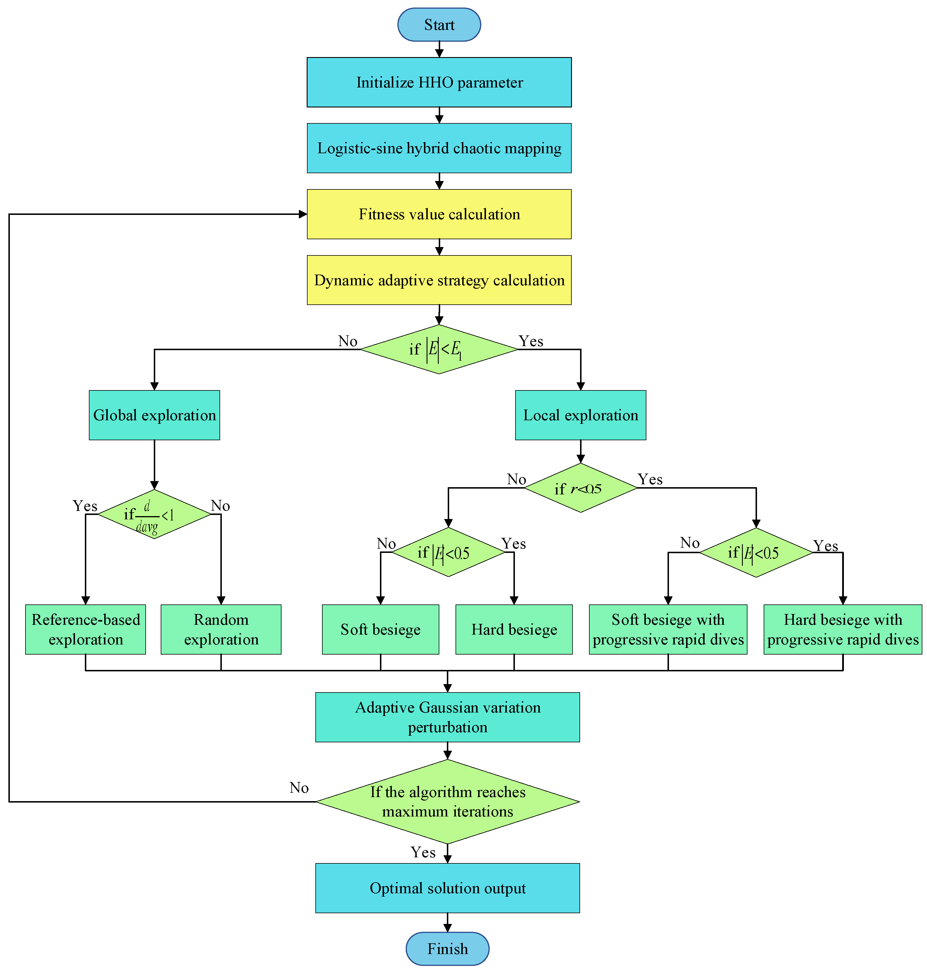
2.1. The Principle of the HHO Algorithm

The HHO algorithm which proposed by Heidari et al. is a novel intelligent optimization algorithm inspired by the foraging and hunting behaviors of Harris hawks that is the only social birds of hawks [26]. Unlike traditional algorithms, the HHO algorithm does not rely on the analytical properties of the objective function and imposes minimal constraints on the initial point. Compared to other intelligent algorithms such as Particle Swarm Optimization and Differential Evolution, HHO offers several advantages, including fewer parameters, simpler structure, faster convergence, and enhanced local search capability [28]. The algorithm simulates the foraging and hunting strategies of Harris hawks, treating prey as the optimal solution and the Harris hawks as the candidate solution, and is divided into exploration and exploitation phases [29].

2.1.1. Exploration Phase

The algorithm performs global exploration at this phase. Harris hawks are randomly distributed in the solution space to search for prey, updating their location according to two strategies: randomly perching on trees or positioning based on the location of other hawks and prey. The strategy is chosen based on random number $q$ and the position can be expressed as:

$$X\left(t+1\right)=\left\{\begin{array}{c}{X}_r\left(t\right)-c_1\left|X_r\left(t\right)-2\times c_{2}X\left(t\right)\right| q\ge 0.5\\ \\ \left(X_{prey}\left(t\right)-X_m\left(t\right)\right)-c_3\left(lb+c_4\left(ub-lb\right)\right) q<0.5\end{array}\right.$$

(1)

where $X(t+1)$ represents the next iteration position of the hawk, $X\left(t\right)$, $X_m\left(t\right)$, $X_r\left(t\right)$ and $X_{prey \left(t\right)}$ are the current position, average position, random position of hawk and the prey position, respectively. t is the current iteration number. $c_1$, $c_2$, $c_3$ and $c_4$ are the random numbers between 0 and 1. $ub$ and $lb$ represent the lower limit and upper limit of the solution space, respectively. The average position can be expressed as:

$$X_m\left(t\right)={\displaystyle \frac{1}{N}}\sum _{i=1}^N X_i\left(t\right)$$

(2)

In this case, $N$ is the population size and $X_i\left(t\right)$ is the position of the $i \mathrm{t}\mathrm{h}$ hawk in the current iteration.

2.1.2. Switch Between Exploration and Exploitation Phases

The switch between exploration and exploitation phases is governed by the energy $E_{prey}$ and is expressed as:

$$E_{prey}=2E_0\left(1-{\displaystyle \frac{t}{t_{max}}}\right)$$

(3)

where $t_{max}$ is the maximum number of iteration and $t$ is the current number of iterations. $E_0$ is a random number representing initial energy and $E_0\in (-\mathrm{1,1})$.

2.1.3. Exploitation Phase

The algorithm performs global exploration at this phase. The besiege strategy is chosen according to the energy of prey $E_{prey}$ and possibility of escaping $r$. If $\left|E\right|<0.5$ the hard besiege strategy is adopted; otherwise, the soft besiege strategy is applied. Additionally, if $r<0.5$, the prey successfully escapes, whereas for $r\ge 0.5$, the prey fails to escape. Consequently, there are four possible position-updating strategies.

(1)

Soft besiege

When $\left|E\right|\ge 0.5$ and $r\ge 0.5$, the prey retains enough energy and attempts random leaps to mislead the hawks but ultimately fail to escape. Consequently, the soft besiege strategy is deployed for a sudden attack. The current position of hawks can be updated as:

$$X\left(t+1\right)=X_{best}\left(t\right)-X\left(t\right)-E_{prey}\mid J{X}_{best}\left(t\right)-X\left(t\right)\mid$$

(4)

$J$ is the jumping intensity and can be expressed as:

$$J=2\left(1-c_5\right)$$

(5)

$c_5$ is a random number updated at each iteration, satisfying $C_5\in \left(\mathrm{0,1}\right)$.

(2)

Hard besiege

When $\left|E\right|<0.5$ and $r\ge 0.5$, the prey has low energy to escape besiege. Hawks hardly surrounds the prey but conducts a sudden attack. The position of hawks is updated as:

$$X\left(t+1\right)=X_{best}\left(t\right)-E_{prey}\mid X_{best}\left(t\right)-X\left(t\right)\mid$$

(6)

(3)

Soft besiege with progressive rapid dives

When $\left|E\right|\ge 0.5$ and $r<0.5$, the prey has sufficient energy to escape successfully. Hawks will adopt soft besiege with progressive rapid dives to narrow the distance of the prey. The mathematical model can be established as:

$$X\left(t+1\right)=\left\{\begin{array}{c}Y,F\left(Y\right)<F\left(X\right(t\left)\right)\\ \\ Z,F\left(Z\right)<F\left(X\right(t\left)\right)\end{array}\right.$$

(7)

$$Y=X_{best}\left(t\right)-E_{prey}\mid J{X}_{best}\left(t\right)-X\left(t\right)\mid$$

(8)

$$Z=Y+S\times Levy\left(dim\right)$$

(9)

Herein, $dim$ is the dimension of optimization problem, and $S$ represents a random vector with the dimension of $1\times dim$. $Levy\left(dim\right)$ is the Levy fling function which can be expressed as:

$$LF\left(x\right)=0.01\times {\displaystyle \frac{u\times \sigma }{|v{|}^{\frac{1}{\beta }}}}$$

(10)

μ and υ are random numbers between 0 and 1, β is a content which is empirically set to 1.5. σ can be calculated by:

$$\sigma ={\left({\displaystyle \frac{\mathsf{\Gamma }\left(1+\beta \right)\times \sin \left(\frac{\pi \beta }{2}\right)}{\mathsf{\Gamma }\left(\frac{1+\beta }{2}\right)\times \beta \times 2^{\left(\frac{\beta -1}{2}\right)}}}\right)}^{{\displaystyle \frac{1}{\beta }}}$$

(11)

(4)

Hard besiege with progressive rapid dives

When $\left|E\right|<0.5$ and $r<0.5$, the prey has insufficient energy, but still has a chance to escape. Therefore, the Harris eagle adopts a hard siege with progressive rapid dives to narrow the distance with the prey. Its mathematical model is shown as:

$$X\left(t+1\right)=\left\{\begin{array}{c}Y,F\left(Y\right)<F\left(X\right(t\left)\right)\\ \\ Z,F\left(Z\right)<F\left(X\right(t\left)\right)\end{array}\right.$$

(12)

$$Y=X_{best}\left(t\right)-E_{prey}\mid J{X}_{best}\left(t\right)-X_m\left(t\right)\mid$$

(13)

$$Z=Y+S\times Levy\left(dim\right)$$

(14)

2.2. The Optimization of the HHO Algorithm

The HHO algorithm is a novel swarm intelligence algorithm inspired by the cooperative hunting behavior of Harris hawks. While HHO benefits from a straightforward mechanism, fewer control parameters, and ease of implementation, it suffers from drawbacks including low convergence accuracy, slow convergence rate, and susceptibility to local optima [30]. To address these limitations, the paper proposes a novel HHO algorithm.

2.2.1. Circle Chaotic Mapping

Chaotic sequences can be deployed to initialize the hawk population positions in an HHO algorithm, effectively alleviating the issues such as overly dense individual aggregation and insufficient population diversity during the initial stage. Firstly, a set of chaotic sequences is generated by circular chaotic mapping to initialize the population positions, so that individuals are uniformly distributed in the search space and enhance the global exploration ability of the algorithm; subsequently, the decision variables are introduced into the chaotic variable space by nonlinear mapping. With the help of the ergodicity and randomness of chaos, the diversity of the initial population is further enhanced. Finally, the obtained chaotic variables are mapped back to the feasible solution space of the optimization problem by using linear transformation. This process effectively expands the distribution range of the initial solution and provides a better starting point for the subsequent evolutionary search. Compared to other common chaotic maps such as Logistic, Tent, or Sine maps, the Circle chaotic map exhibits better balance between randomness and distribution uniformity. It has a relatively simple structure but demonstrates excellent ergodicity and low correlation, which make it particularly effective in avoiding premature convergence and maintaining search diversity in high-dimensional spaces. In our tests, the Circle map achieved more uniform coverage of the solution space during initialization, leading to improved convergence stability of the HHO algorithm. Therefore, it was selected for initializing the hawk population in this study. The circle chaotic mapping is expressed as:

$$X(t+1)=\mathrm{m}\mathrm{o}\mathrm{d}\left(X\left(t\right)+K-\left({\displaystyle \frac{\mu }{2\pi }}\right)\sin \left(2\pi X\left(t\right)\right),1\right)$$

(15)

$K$ and $\mu$ are control parameters which are empirically set to 0.5 and 0.2, respectively.

2.2.2. Dynamic Adaptive Escape Energy

When the iteration number proceed, the prey energy $E_{prey}$ remains consistently below 1, causing the algorithm to become restricted to the exploration phase. In addition, $E$ changes in linear decrease ways which limit the balance ability between global optimization and local exploitation. This method introduces a dynamic adaptive weight strategy to increase the nonlinearity expression of prey escape energy, which enhances the global optimization and local exploitation accuracy. This method sets the parameter $E_1$ through a nonlinear decreasing mechanism and models the variation trend using the cosine function. When $E\ge E_1$, the algorithm adopts global exploration, otherwise it will conduct local exploitation phase. The adaptive escape energy can be expressed as:

$$E=E_0{E}_1$$

(16)

$$E_1=E_0\left({\displaystyle \frac{{\omega }_{max}-{\omega }_{min}}{2}}\cos \left({\displaystyle \frac{\pi t}{T}}\right)+{\displaystyle \frac{{\omega }_{max}+{\omega }_{min}}{2}}-{\omega }_{min}\right)$$

(17)

Herein, ${\omega }_{max}$ and ${\omega }_{min}$ are 2.1 and 0.1, respectively.

2.2.3. Improvement of Exploration Phase

The update law of individual position depends on the random number $q$ in the exploration phase. When $r\ge 0.5$, the algorithm employs a random exploration strategy, resulting in relatively large updates to individual positions, thereby effectively expanding the search space. When $r<0.5$, individuals implementing the reference exploration strategy exhibit limited update range. However, the following situation may occur during the exploration process: (1) The hawk is close to the prey but $r\ge 0.5$, (2) The hawk is far from the prey but $r<0.5$.

When the hawk population is close to the prey, more precise position update should be conducted based on the both the prey and other individuals to enhance the exploitation ability of the algorithm. However, due to the random number $r\ge 0.5$, individuals prefer random exploration strategy, resulting in excessively divergent behaviors. Conversely, when hawks are far from the prey, more effective besiege strategy should be adopted to enhance global exploration. In contrast, because of the $r<0.5$, individuals conducting the exploration strategy guided by the reference exhibit limited update range, which hinders the algorithm to escape from local optima. The conventional update method is prone to cause waste of exploration resource and affect the optimization efficiency due to the mismatch of individual status. The proposed method introduces information navigation based on average range in the exploration phase and adaptively selects update strategy according to the relative distance between the individual and the prey, in order to improve the search rationality and efficiency of the algorithm in different phases. In the new method, the random number $d_{a\nu g}$ is replace by $d\left(X_i\right)/d_{a\nu g}$. The update law can be expressed as:

$$X\left(t+1\right)=\left\{\begin{array}{c}{X}_r(t)-c_1\left|X_r\left(t\right)-2\times c_{2}X\left(t\right)\right| {\displaystyle \frac{d}{d_{a\nu g}}}\ge 1\\ \\ (X_{prey}(t)-X_m(t))-c_3\left(LB+c_4\left(ub-lb\right)\right){\displaystyle \frac{d}{d_{a\nu g}}}<1\end{array}\right.$$

(18)

Under this circumstance,$d_{a\nu g}$ is the average distance between the hawks and the prey. The $d\left(X_i\right)$ and $d_{a\nu g}$ can be calculated as:

$$d\left(X_i\right)=∥X_i-X_{prey}∥$$

(19)

$$d_{a\nu g}={\displaystyle \frac{1}{N}}\sum _{i=1}^N d\left(X_i\right)$$

(20)

2.2.4. Adaptive Mutation Strategy

In order to address the tendency of the HHO algorithm to become trapped in local optima, the proposed method deploys a Gaussian mutation mechanism to introduce a disturbance which incorporates with the normal distribution to the initial position. This approach generates a mutated position and tends to favor the solution in the vicinity of the original position, which enhances the local search capability of the algorithm. As a result, Gaussian mutation contributes to improving the optimization accuracy, mitigating premature convergence, and accelerating convergence speed. The Gaussian probability density function is expressed as:

$$g\left(x\right)={\displaystyle \frac{1}{\sqrt{2\pi }\sigma }}\exp \left(-{\displaystyle \frac{(x-\mu {)}^2}{2{\sigma }^2}}\right)$$

(21)

where $\mu$ and $\sigma$ are the mean and standard deviations, which are usually set to 0 and 1, that is, the standard normal distribution function. Therefore, a Gaussian calculation operator is proposed and can be shown as:

$$G_0=G\left(i\right)\left(X_{r1}-X_{r2}\right)$$

(22)

$G\left(i\right)$ is a random number generated by Gaussian density function. $X_{r1}$ and $X_{r2}$ are the two random individuals in the population.

Correspondingly, if the random number in the Gaussian mutation follows the uniform distribution, then the generated mutation strategy is called uniform mutation and is expressed as:

$$U_0=U\left(i\right)\left(X_{r1}-X_{r2}\right)$$

(23)

$U\left(i\right)$ is the position of hawk before mutation. By comparing the position of the two hawks and retaining the best position, the final position is shown as:

$$h\left(x\right)=\left\{\begin{array}{c}{\displaystyle \frac{1}{b-a}} a<x<b\\ 0 else\end{array}\right.$$

(24)

where the $a$ and $b$ are the fitness functions which render $h\left(x\right)$ become uniform distribution.

The article proposes an adaptive mutation strategy where the new position after mutation is shown as:

$$X_{new}=\left\{\begin{array}{c}{U}_0+X_{old} \left|E\right|\ge E_1\\ G_0+X_{old} \left|E\right|<E_1\end{array}\right.$$

(25)

where $X_{old}$ is the hawk position before mutation. The final position is determined by comparing the position of two hawks and can be expressed as:

$$X\left(t+1\right)=\left\{\begin{array}{c}{X}_{new},f\left(X_{new}\right)<f\left(X_{old}\right)\\ X_{old},f\left(X_{new}\right)\ge f\left(X_{old}\right)\end{array}\right.$$

(26)

$f(·)$ is the fitness function.

In the adaptive mutation strategy, when the prey escape energy satisfies $\left|E\right|\ge E_1$, the uniform mutation is adopted, otherwise the Gaussian mutation dominantes. Therefore, the novel HHO algorithm achieves a broader global exploration by deploying uniform mutation at the early stage of the search. In the later stage of the search, Gaussian mutation not only allows the algorithm to escape the local optima, but also ensures a relatively high convergence rate. Compared to other perturbation strategies such as polynomial mutation or Cauchy mutation, Gaussian mutation offers a balanced trade-off between local exploitation and computational simplicity. Polynomial mutation tends to generate broader perturbations, which is useful for exploration but may reduce fine-tuning precision in later stages. Cauchy mutation, although capable of generating long jumps, often introduces instability due to heavy-tailed distribution. In contrast, Gaussian mutation produces moderate, normally distributed variations that concentrate around the current solution, making it more suitable for enhancing exploitation without significantly disturbing convergence. In our experiments, Gaussian mutation exhibited better stability and faster convergence when integrated with the HHO framework, especially during the local exploitation phase where precise refinement is needed. Therefore, it was chosen as the dominant mutation strategy in the proposed adaptive mechanism.

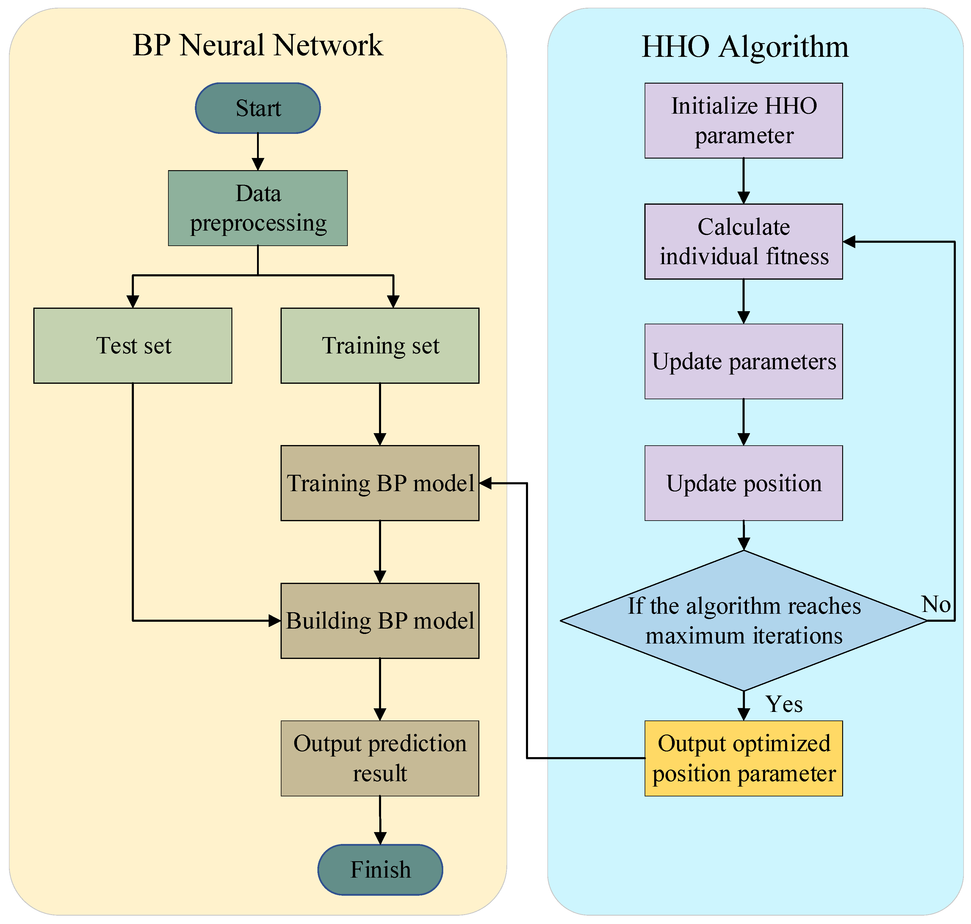
2.3. BP Neural Network Based on the Novel HHO Algorithm

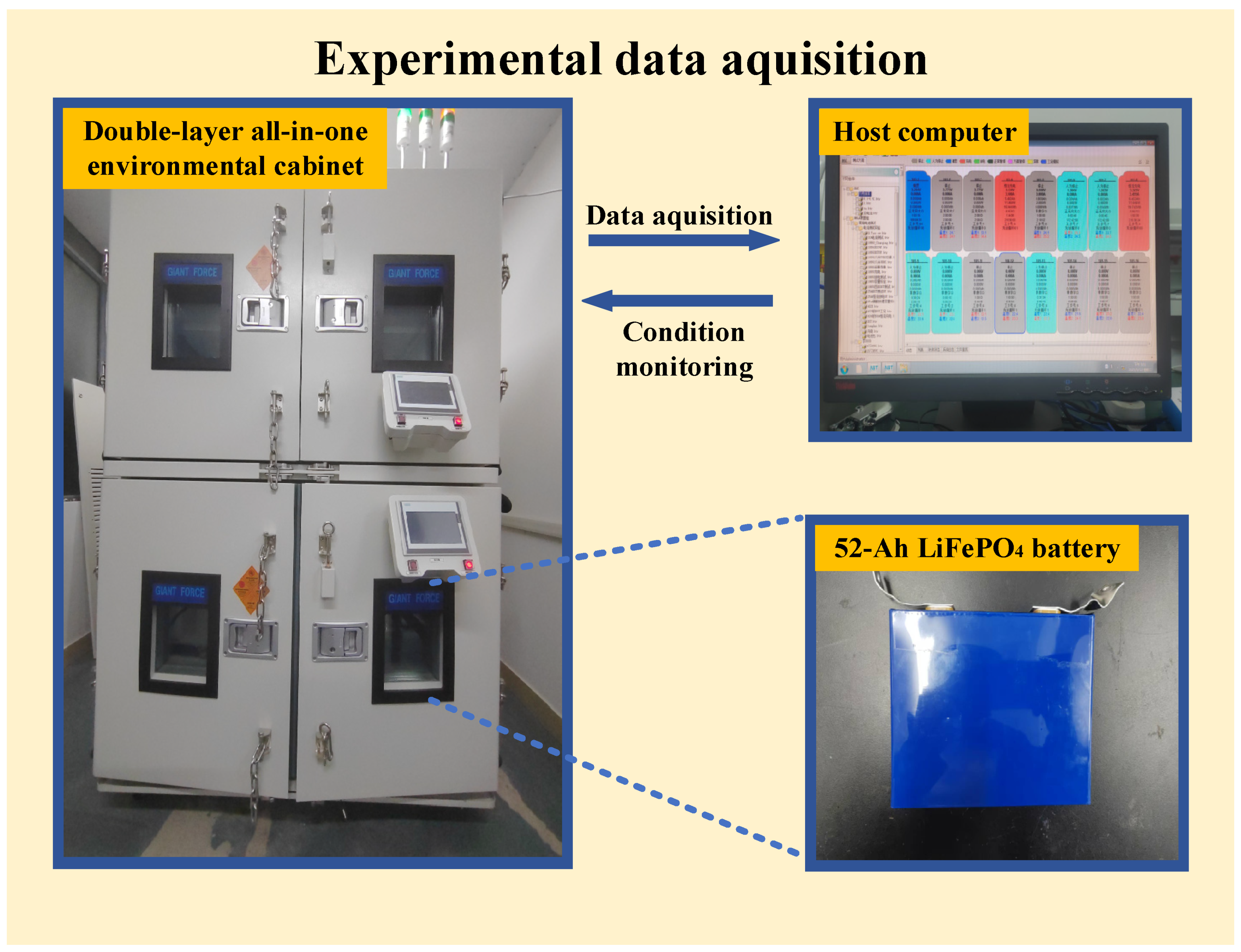
The BP neural network is a multi-layer feedforward network characterized by forward signal propagation and backward error correction through gradient descent [31]. By learning the data mapping relationships during training, it exhibits strong generalization capability and effectively captures the nonlinear degradation behavior of battery capacity over its entire lifecycle. However, the BP neural network also suffers from limitations, particularly with respect to sensitivity to initial parameter settings. To address this issue, a novel HHO–BP algorithm is employed in this study to optimize the weights and biases of the BP neural network. Based on this enhancement, an improved BP neural network model for RUL prediction is developed. The corresponding framework is illustrated in Figure 1.

3. Experiment

3.1. Evaluation of Health Factors

Common parameters used to characterize battery aging include capacity and impedance, which are considered direct health factors and play a critical role in predicting the remaining useful life of batteries. Although capacity can theoretically be estimated by measuring discharge time under constant current, this is difficult to achieve in real-world scenarios. In practical applications, maintaining a stable constant current over the entire usable capacity range is often infeasible due to dynamic load conditions, safety constraints, or time limitations. Similarly, measuring internal resistance accurately requires specialized equipment such as electrochemical impedance spectroscopy or pulse testing, which is costly and not feasible for online monitoring.

Given these limitations, it becomes essential to identify features that are easy to obtain during regular electrochemical operations and can serve as reliable proxies for capacity. Among indirect health indicators, incremental capacity analysis and internal resistance are widely used. However, incremental capacity analysis relies on high-resolution data and is extremely sensitive to noise and temperature fluctuations, limiting its applicability in online or embedded systems. Internal resistance measurement also requires dedicated test procedures, which are difficult to implement under standard operating conditions of electric vehicles.

In contrast, the time it takes for battery voltage to rise or fall between two predefined voltage thresholds under constant current conditions can be easily extracted from routine charge and discharge data. This type of time-based feature requires no additional hardware, fits seamlessly with real-world operating profiles, and is less affected by environmental disturbances. Experimental results and grey relational analysis confirm that these time indicators strongly correlate with battery capacity and aging behavior. Therefore, they provide a practical, cost-effective, and reliable alternative for online health estimation in real-world applications

To ensure that health factors accurately represent battery capacity, grey relational analysis is utilized to examine the correlation between these factors and capacity. This method assesses the inter-element correlation by quantitatively analyzing various indicators and deriving the grey relational degree. The specific calculation steps are as follows:

(1)

Determine the analysis series: Designate the battery capacity as the reference sequence $y\left(k\right)$, and the extracted health factors as the comparative sequences $x_i\left(k\right)$;

(2)

Calculate the correlation coefficients:

$${\xi }_i\left(k\right)={\displaystyle \frac{\underset{i}{min} \underset{k}{min} \left|y\left(k\right)-x_i\left(k\right)\right|+\rho \underset{i}{max} \underset{k}{max} \left|y\left(k\right)-x_i\left(k\right)\right|}{\left|y\left(k\right)-x_i\left(k\right)\right|+\rho \underset{i}{max} \underset{k}{max} \left|y\left(k\right)-x_i\left(k\right)\right|}}$$

(27)

where $\rho$ is resolution coefficient and usually set to 0.5;

(3)

Calculate the correlation degrees.

The value of the correlation coefficient indicates the relationship between each health factor and capacity across various cycles, which makes an overall comparison challenging. Hence, it is essential to aggregate these values and compute their mean. In that case, a single metric can be utilized to evaluate the association between health factors and capacity. The formula for the correlation degree $r_i$ is as follows:

$$r_i={\displaystyle \frac{1}{n}}\sum _{k=1}^n{\xi }_i\left(k\right)$$

(28)

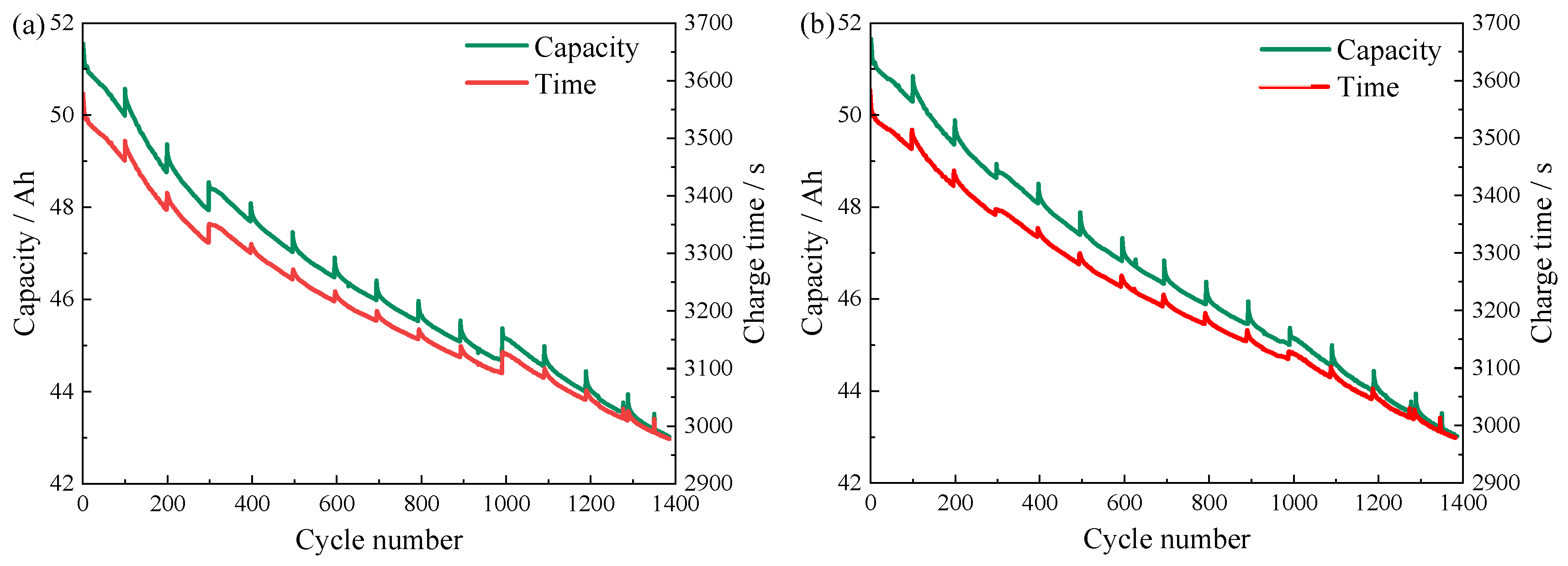
3.2. Battery Aging Data and Health Factor Extraction

The experimental battery adopts a commercial 52-Ah LiFePO₄ battery with a rated voltage of 3.2 V. And the detailed parameters are shown in

Table 1. Basic parameters of the experimental cell.

Parameters	Value/Composition
Geometric dimensions L × W × H (mm × mm × mm)	148 × 27 × 115
Rated voltage/V	3.2
Rated capacity/Ah	52
Operating Voltage/V	2.5~3.65
Anode	Graphite
Cathode	LiFePO4

. The testing setup comprises a battery testing system, an LW-150 high- and low-temperature test chamber, and a supervisory computer, as depicted in Figure 2.

At a set temperature of 25 °C, the new battery is first charged at a constant current of 1 C until the voltage reaches 3.65 V. After 20 min, the battery is discharged with a constant current of 1 C until the voltage achieves 2 V. The charge–discharge steps are repeated until the battery capacity declines to 80% of its rated capacity, at which point the test is terminated.

Although the operating voltage specified in Table 1 is 2.5–3.65 V, the lower cut-off voltage was intentionally set to 2.0 V during the aging experiment. This decision was made to accelerate the degradation process and shorten the experimental duration, which is a common practice in battery aging studies. Extending the depth of discharge increases the electrochemical stress on electrode materials, allowing capacity fade mechanisms to manifest more rapidly. While this does exceed the nominal range, the approach remains within the tolerable limits for experimental purposes and does not compromise the validity of the observed aging trends.

During the charging process, the battery voltage may reach the preset cut-off value before lithium ions are fully intercalated into the electrode materials, resulting in a discrepancy between the surface and actual states of charge. Implementing a resting period after charging allows additional time for lithium ions to diffuse uniformly toward the electrode surfaces, thereby achieving a state closer to full charge. This process also mitigates the effects of transient overvoltage caused by the differing transport rates of ions and electrons, reduces polarization, and helps to stabilize the electrochemical state of the battery prior to the subsequent charge–discharge cycle. Meanwhile, during the rapid charging and discharging processes, the battery temperature will rise. Leaving it on hold helps the battery dissipate heat, allowing the temperature to return to a level close to the environment and preventing further temperature accumulation that could affect the safety of the experiment or the reliability of the data. This manifests as a slight capacity rebound, which is often observed in long-term cycling studies, particularly under controlled temperature and fixed cycling conditions. The high regularity of these spikes may result from the thermal management and shelving design used in the experiment, which provides a consistent opportunity for internal relaxation and recovery approximately every 100 cycles. Importantly, these spikes do not disrupt the overall downward trend of capacity degradation and are considered part of the natural fluctuation behavior during aging. Due to the relaxation effect during this rest period, the open-circuit voltage typically rose to around 3.15 V. Therefore, although the discharge cut-off was set to 2 V, the actual charging process under constant current started from the relaxed voltage of ~3.15 V up to 3.65 V. Finally, in actual use, batteries are not always in a working state. On the contrary, they often have idle states such as standby or backup. Adding a shelving stage in the experiment helps to better simulate the actual working conditions and improve the representativeness of the experimental data.

During the constant-current charging process, the voltage curve exhibits a relatively smooth and stable time when it rises from 2 V to 3.65 V, indicating consistent behavior across charge cycles. This stability makes the corresponding time interval a suitable candidate for healthy indicator. Accordingly, the time required for the voltage to increase from 2 V to 3.65 V under constant charging current is selected as a health factor to characterize battery capacity. Figure 3 shows the charging time difference and capacity attenuation of batteries B1 and B2 at the same voltage rise. As the number of charge–discharge cycles increases, the battery undergoes aging, resulting in a gradual decline in the battery available capacity. Under the constant-current charging condition, this reduction in capacity leads to a corresponding decrease in charging time. Ideally, under strict constant current (CC) conditions, the capacity can be computed as the product of current and time, implying a direct proportionality between charging time and capacity. However, in practice, several factors such as changes in internal resistance, side reactions, cut-off thresholds, and measurement noise introduce deviations from perfect proportionality. This explains why, although the green and red curves in Figure 3 (charging time vs. capacity) show high correlation, they are not strictly proportional.

During the constant current discharge stage, the battery voltage exhibited a gradual and relatively stable decline from 3.65 V to 2 V, indicating consistent discharge behavior across multiple cycles. The stable voltage reduction interval provides a robust basis for battery health assessment. Consequently, the time required for the voltage to decrease from 3.65 V to 2 V under constant current discharge conditions was selected as the health indicator reflecting the battery’s capacity state. As is shown in Figure 4, the discharge time curve of batteries B1 and B2 closely align with their respective capacity degradation curves. Especially during the stage of capacity regeneration, both curves maintain a consistent trend. Again, although discharge time is theoretically proportional to capacity under ideal CC discharge, practical inconsistencies due to real-world aging effects and system dynamics can lead to slight mismatches. Nevertheless, the high correlation validates its use as a reliable health indicator. This indicates that discharge time can effectively reflects changes in capacity and can serve as a key indicator for accessing battery health status.

The grey correlation degree analysis is conducted between charging (discharging) time during the same voltage range and the battery capacity, based on the aging test data of the batteries. The results are shown in

Table 2. Correlation of relevant health factor.

Variable	B1 Charging Time/s	B1 Discharging Time/s	B2 Charging Time/s	B2 Discharging Time/s
GRA	0.954	0.954	0.951	0.951

. The correlation meets the requirements, indicating that the selected health factors can well characterize the battery capacity.

The charging and discharging time during the same voltage range of the battery were taken as input variables, where the normalized data was subjected to polynomial regression fitting for the battery capacity. The resulting fitting curves for charging (discharging) time during the same voltage range under the constant current versus battery capacity are shown in Figure 3 and Figure 4, respectively. The overall fitting effectiveness is evaluated using the accommodation coefficient ($R^2$) and the root mean square error (RMSE). The formula for $R^2$ is as follows:

$$R^2=1-{\displaystyle \frac{\sum _{i=1}^n{\left(y\left(x_i\right)-\widehat{y}\left(x_i\right)\right)}^2}{\sum _{i=1}^n{\left(y\left(x_i\right)-\overline{y}\left(x_i\right)\right)}^2}}$$

(29)

The true values and fitted values are denoted by $y\left(x_i\right)$ and $\widehat{y}\left(x_i\right)$, respectively. The average of true values is represented by $\overline{y}\left(x_i\right)$.

Figure 5 illustrates the fitting curve for constant-current charge (discharge) time and battery capacity. The fitted curves closely match the original capacity curves, as illustrated in

Table 3. Fitting of relevant health factor correlation.

Variable	B1 Charging Time/s	B1 Discharging Time/s	B2 Charging Time/s	B2 Discharging Time/s
$R^2$	0.99	0.99	0.99	0.99
RMSE	0.028	0.0042	0.026	0.0069

. Specifically, the linear fitting between constant-current charging time and capacity achieved an R² of 0.99 with RMSE of 0.028 and 0.0042, and the fitting for constant-current discharge voltage drop time versus capacity produced an R² of 0.99 with RMSE of 0.026 and 0.0069. The results indicate a strong linear correlation between battery capacity and both the constant-current charging time, and the constant-current discharge drop time. These time-based features exhibit a high degree of correlation with capacity degradation and can be effectively used as health indicators to characterize battery aging and performance attenuation. In general, the proposed two health factors effectively characterize battery capacity, exhibiting low error in linear fitting with battery capacity and maintaining consistency with the battery capacity degradation curve.

3.3. RUL Prediction Process

The complete workflow of RUL prediction model, based on the BP neural network optimized by the novel HHO algorithm, is illustrated in Figure 6. The methodology includes the following steps: (1) Data preprocessing is conducted by utilizing raw data from aging tests of 52-Ah LiFePO₄ batteries. Charge–discharge data is extracted from the original dataset, after which the data is segmented into training and testing subsets. (2) Health factor extraction is performed. Health indicators are derived from key parameters collected during battery charging, including voltage, current, temperature, and charging duration. The extracted factors undergo correlation assessment using grey relational analysis to form an optimized input feature set. (3) A prediction model is constructed. The weights and biases of the BP neural network serve as optimization targets, optimized through the improved HHO algorithm to enhance prediction performance. (4) RUL prediction is realized by feeding the constructed input feature set into the optimized neural network, which outputs predicted RUL of the battery. The accuracy and effectiveness of the proposed model are validated through standard evaluation metrics.

4. Results and Discussion

4.1. Verification Setup

In order to verify the effectiveness of the proposed algorithm, the experiments are carried out by comparing the performance of BP neural network, HHO–BP neural network and the novel HHO–BP neural network. The two healthy factors are set as the input and the battery RUL is the output of the neural network. The first 50~70% of the cycle data is used as the training set while the rest are the testing sets for RUL estimation. To evaluate the estimation performance, three metrics are employed, namely mean square error (MAE), root mean square error (RMSE) and mean absolute percentage error (MAPE). These metrics serve as the evaluation functions, and their respective formulations are given as:

$$MAE={\displaystyle \frac{1}{N}}\sum _{i=1}^N \left|y_i-{\widehat{y}}_i\right|$$

(30)

$$RMSE=\sqrt{{\displaystyle \frac{1}{N}}\sum _{i=1}^N (y_i-{\widehat{y}}_i{)}^2}$$

(31)

$$MAPE={\displaystyle \frac{1}{N}}\sum _{i=1}^N \left|{\displaystyle \frac{y_i-{\widehat{y}}_i}{y_i}}\right|\times 100\%$$

(32)

$N$ is the battery total cycle number, $y_i$ is the real value of RUL and ${\widehat{y}}_i$ is the estimation value.

4.2. Experimental Result Analysis

For ease of expression, the four optimization strategies in Section 3.2 are, respectively, denoted as “Scheme 1” to “Scheme 4”, and the naming conventions of the corresponding optimization models are shown in

Table 4. Optimization strategy combination.

Optimization Scheme	Model Name
Scheme 1	N1
Scheme 1 and Scheme 2	N2
Scheme 1, Scheme 2, and Scheme 3	N3
Full optimization	N4

.

The RUL estimation results of different model considering the battery aging process are shown in Figure 7.

As illustrated in Figure 7 and Figure 8, and

Table 5. Comparison of evaluation indexes of different models.

Battery	Training Set	Model	RMSE	MAPE	MAE	Run Time/s
B1	70%	BP	0.0649	0.0282	0.0467	6.115
		HHO–BP	0.0575	0.0261	0.0411	287.120
		N1	0.0404	0.0273	0.0341	276.670
		N2	0.0279	0.0165	0.0187	292.691
		N3	0.0273	0.0137	0.0231	227.668
		N4	0.0164	0.0044	0.0114	231.555
	60%	BP	0.0884	0.0507	0.0375	6.002
		HHO–BP	0.0684	0.0315	0.0289	291.332
		N1	0.0436	0.0236	0.0242	256.989
		N2	0.0331	0.0259	0.0161	236.518
		N3	0.0262	0.0142	0.0106	243.107
		N4	0.0095	0.0089	0.0044	225.454
	50%	BP	0.0888	0.0282	0.0524	6.897
		HHO–BP	0.0771	0.0261	0.0462	279.639
		N1	0.0429	0.0273	0.0393	256.132
		N2	0.0340	0.0171	0.0187	282.197
		N3	0.0191	0.0199	0.0231	238.428
		N4	0.0069	0.0095	0.0114	236.733
B2	70%	BP	0.0686	0.0414	0.0455	6.638
		HHO–BP	0.0551	0.0292	0.0406	284.092
		N1	0.0375	0.0218	0.0423	274.322
		N2	0.0322	0.0169	0.0248	294.510
		N3	0.0177	0.0106	0.0240	221.563
		N4	0.0158	0.0069	0.0093	230.143
	60%	BP	0.0885	0.0676	0.0576	6.217
		HHO–BP	0.0748	0.0312	0.0422	290.848
		N1	0.0336	0.0245	0.0238	259.163
		N2	0.0410	0.0267	0.0293	258.164
		N3	0.0273	0.0106	0.0224	229.888
		N4	0.0116	0.0031	0.0060	228.334
	50%	BP	0.0772	0.0251	0.0548	5.845
		HHO–BP	0.0465	0.0265	0.0421	283.726
		N1	0.0375	0.0316	0.0252	293.523
		N2	0.0376	0.0169	0.0366	257.839
		N3	0.0245	0.0184	0.0245	231.567
		N4	0.0135	0.0094	0.0096	234.888

, the novel HHO–BP neural network demonstrates superior performance in predicting the RUL under varying training dataset proportions. Under a 70% training dataset proportion, the MAE for predicted values of batteries B1 and B2 are less than 0.012, the RMSE are maintained below 0.017, and the MAPE are approximately 0.7%. Relative to the traditional BP neural network, the proposed model achieves reductions in MAE by approximately 0.035, RMSE by 0.050, and MAPE by 2.4% and 3.5%, respectively. Compared with the HHO–BP neural network, the novel HHO–BP method further decreases MAE by 0.029 and 0.031, RMSE by 0.041 and 0.053, and MAPE by 2.2% and 2.3% for B1 and B2, respectively. Traditional BP neural networks are constrained by inherent gradient optimization limitations, leading to significantly higher prediction errors and lower stability compared to optimized models. Although the HHO–BP model partially addresses parameter convergence through its global search mechanism, challenges persist in computational efficiency and local optimization accuracy. The systematic integration of strategies N1 through N4 progressively strengthens the overall performance of the model. Strategy N1 employs chaotic mapping to effectively enhance search space coverage and mitigate biases in population initialization. Strategy N2 introduces a dynamic adaptive escape energy mechanism that accelerates convergence and reduces oscillation by balancing exploration and exploitation phases adaptively. Strategy N3 optimizes parameter updating pathways through refined decision-making, significantly enhancing the capability to escape local extrema. Finally, strategy N4 incorporates an adaptive mutation mechanism to further improve the adaptability to non-stationary characteristics such as capacity regeneration, thus achieving simultaneous enhancements in prediction accuracy and robustness.

For the 60% training dataset proportion, the MAE for both B1 and B2 remain below 0.006, with RMSE values contained within 0.012 and MAPE under 0.9%. Compared to the conventional BP neural network, MAE reductions are 0.033 and 0.051, RMSE reductions are 0.079 and 0.077, and MAPE improvements reached 4% and 6% for B1 and B2, respectively. Furthermore, relative to the HHO–BP neural network, the proposed method yields reductions in MAE of 0.024 and 0.036, RMSE by 0.059 and 0.063, and MAPE by 2.3% and 2.8% for B1 and B2, respectively. Data reduction exacerbates overfitting risks in traditional BP neural networks, resulting in substantial increases in prediction error fluctuations. While the fundamental HHO–BP model mitigates initial value dependencies through multi-agent cooperative optimization, its fixed population update rules tend to converge prematurely under small-sample conditions. The hierarchical optimization provided by strategies N1–N4 significantly improves model adaptability under data scarcity. Strategy N1 increases population diversity to enhance noise suppression capability. Strategy N2 dynamically adjusts search intensity to alleviate convergence instability caused by insufficient data. Strategy N3 optimizes local search path weights, thereby improving parameter updating efficiency. Strategy N4 employs an adaptive mutation mechanism to effectively capture early degradation features, maintaining high generalization performance even with limited data.

At a 50% training dataset proportion, the MAE for B1 and B2 predictions was consistently below 0.012, RMSE values are less than 0.014, and MAPE remained within 0.95%. Compared to traditional BP neural network predictions, the MAE decreased by 0.051 and 0.045, RMSE reductions are approximately 0.081 and 0.064, and MAPE improved by 1.9% and 1.5%, respectively. Compared with the conventional HHO–BP neural network, the novel HHO–BP method shows additional MAE reductions of 0.035 and 0.033, RMSE reductions of 0.070 and 0.033, and a MAPE decrease of approximately 1.7%. Small-sample scenarios reveal inherent deficiencies of traditional BP and HHO–BP models; the former suffers from amplified prediction bias due to gradient vanishing, and the latter struggles with adaptability to highly uncertain degradation trajectories due to fixed optimization strategies. Under such constraints, the coordinated optimization strategies N1–N4 demonstrate substantial engineering value. The global search optimization of Strategy N1 effectively prevents models from falling into local suboptimal solutions. Strategy N2 expedites convergence and suppresses iterative oscillations, thereby reducing computational resource consumption. Strategy N3 finely adjusts the exploration–exploitation balance to enhance parameter optimization accuracy. Lastly, strategy N4 incorporates a dynamic mutation mechanism, improving the model’s sensitivity to nonlinear degradation patterns and maintaining stable prediction performance under conditions of highly limited data.

Moreover, the proposed novel HHO–BP neural network method demonstrates significant computational efficiency advantages. The overall convergence time is reduced by approximately 50 s compared to the traditional HHO–BP neural network, underscoring its high operational efficiency and stability while maintaining predictive accuracy.

The model achieves low RMSE, MAE, and MAPE in SOH prediction mainly because of several reasons. The selected features have strong physical correlations with SOH, which helps the neural network establish effective input–output mappings. The model structure is well matched to the data characteristics, with an appropriate parameter dimension that avoids overfitting or underfitting. The training data come from consistent operating conditions or battery types, resulting in relatively stable sequences that make it easier for the model to learn underlying patterns. Additionally, preprocessing techniques such as normalization were applied during training to improve numerical stability. These factors together contribute to the model’s low errors across multiple evaluation metrics.

Although the model achieves low RMSE, MAE, and MAPE in SOH prediction, some residual errors remain due to several factors: noise in experimental data such as sensor inaccuracies and environmental fluctuations affects feature extraction and prediction; the BP neural network is prone to local minima, and although the HHO algorithm alleviates this issue, convergence to suboptimal solutions in high-dimensional parameter spaces is still possible; additionally, numerical precision limitations in computations can cause minor cumulative errors. These factors together contribute to the residual prediction errors observed.

In order to further verify the performance of proposed novel HHO–BP neural network, the result of the model is compared with those of models proposed in the relevant literature. The comparison is shown in

Table 6. Comparison with previous reported works.

Model	MAE	RMSE	MAPE
HHO–BP	0.012	0.016	0.007
ER-BP [32]	0.48	0.609	0.0055
MC-LSTM [33]	0.0173	0.0209	0.0125
HT-LSTM [34]	0.0159	0.0246	0.0103
IMS-TN-FNN [35]	0.0588	0.0699	0.0888

.

Table 6 indicates that Zhang et al. utilized incremental capacity analysis-based BP neural network optimized by elbow rule (ER) algorithm to predict remaining capacities of LIBs, achieving a MAPE of merely 0.55%, although with relatively high MAE and RMSE of 0.48 and 0.609, respectively [32]. Park et al. proposed a multi-channel structure long short-term memory (MC-LSTM), which is flexible for various input types and significantly reduce the number of parameters for better generalization [33]. The prediction errors, measured by MAE, RMSE, and MAPE, are 0.073, 0.0209, and 1.25%, respectively. Rao et al. proposed a hyperparameter-tuned LSTM (HT-LSTM) model for automatic incremental capacity curve analysis and extracted meaningful degradation information, achieving prediction errors (MAE, RMSE, and MAPE) of 0.0159, 0.0246, and 1.03%, respectively [34]. Additionally, Ma et al. developed a transformer network with improved multi-head self-attention (IMS-TN) mechanism to capture the dependencies between features at different positions and a feed-forward neural network (FNN) with fully connected layers and a prediction layer is deployed to estimate the RUL, obtaining prediction errors (MAE, RMSE, and MAPE) of 0.0588, 0.0699, and 8.88%, respectively [35].

Comparatively, the proposed prediction model integrated with a novel HHO algorithm and BP neural network utilizes charging (discharging) time during the same voltage range under the constant current as health indicators, demonstrating superior predictive performance. Additionally, the data acquisition process for the prediction model is simpler in practical engineering applications.

5. Conclusions

In this paper, a prediction model integrating the optimized HHO algorithm with the BP neural network is proposed to address the challenge of accurately predicting the RUL of LIBs. The main contributions of this research are summarized as follows:

(1)

Four optimization strategies are introduced, significantly enhancing both the optimization efficiency and prediction accuracy compared to conventional methods. Specifically, circle chaotic mapping is employed to enhance global search capability. Meanwhile, a dynamic adaptive escape energy mechanism improves convergence speed and stability. Furthermore, an improved exploration phase decision strategy optimizes path selection, thereby increasing convergence accuracy. Lastly, an adaptive mutation strategy enhances adaptability to complex nonlinear problems of the model.

(2)

Using gray relational analysis, the correlations between battery capacity and two critical health indicators, namely charging and discharging time during the same voltage range at the constant current, are quantified, both yielding correlation coefficients greater than 0.95. Employing these indicators as input features effectively addresses practical challenges associated with direct battery capacity measurement, significantly enhancing virtual applicability.

(3)

Comparative experiments utilizing training datasets comprising 50%, 60%, and 70% of battery cycling data confirm the robustness and high accuracy of the proposed model. The results demonstrate the MAE values consistently maintain below 0.012, RMSE values keep below 0.017, and MAPE preserve within 0.95%. Compared to existing benchmark models, the proposed approach offers substantial advantages in accuracy, robustness, and generalization capability.

While the proposed method shows excellent performance under the tested conditions, further studies are needed to explore its applicability across different battery chemistries, ambient temperatures, and higher charge–discharge rates. These factors may influence voltage response and degradation behavior, thereby affecting feature reliability. Future work will aim to validate the model under diverse real-world operating scenarios, which is essential to ensure its robustness and scalability in practical applications.

In summary, the proposed method presents a highly efficient, reliable, and accurate solution for health assessment and RUL prediction of LIBs, showing significant promise for practical engineering applications.

References

1. Zhu, Z.; Chai, X.; Xu, L.; Quan, L.; Yuan, C.; Tian, S. Design and performance of a distributed electric drive system for a series hybrid electric combine harvester. Biosyst. Eng. 2023, 236, 160–174. [Google Scholar] [CrossRef]
2. Zhu, Z.; Zeng, L.; Chen, L.; Zou, R.; Cai, Y. Fuzzy Adaptive Energy Management Strategy for a Hybrid Agricultural Tractor Equipped with HMCVT. Agriculture 2022, 12, 1986. [Google Scholar] [CrossRef]
3. Sun, H.; Jiang, H.; Gu, Z.; Li, H.; Wang, T.; Rao, W.; Wang, Y.; Pei, L.; Yuan, C.; Chen, L. A novel multiple kernel extreme learning machine model for remaining useful life prediction of lithium-ion batteries. J. Power Sources 2024, 613, 234912. [Google Scholar] [CrossRef]
4. Li, T.; Jiao, Y. Revealing the Thermal Runaway Behavior of Lithium Iron Phosphate Power Batteries at Different States of Charge and Operating Environment. Int. J. Electrochem. Sci. 2022, 17, 221030. [Google Scholar] [CrossRef]
5. Zuo, H.; Liang, J.; Zhang, B.; Wei, K.; Zhu, H.; Tan, J. Intelligent estimation on state of health of lithium-ion power batteries based on failure feature extraction. Energy 2023, 282, 128794. [Google Scholar] [CrossRef]
6. Demirci, O.; Taskin, S.; Schaltz, E.; Demirci, B.A. Review of battery state estimation methods for electric vehicles-Part II: SOH estimation. J. Energy Storage 2024, 96, 112703. [Google Scholar] [CrossRef]
7. Liu, Y.; Tian, Y.; Liu, D.; Li, H.; Yi, A.; Wang, Y.; Wang, N.; Pei, L.; Wang, Z.; Jiang, H. A novel dual gated recurrent unit neural network based on error compensation integrated with Kalman filter for the state of charge estimation of parallel battery modules. J. Power Sources 2025, 635, 236508. [Google Scholar] [CrossRef]
8. Zhang, F.; Xu, Z.X.; Wang, M.H. State of health estimation for Li-ion battery using characteristic voltage intervals and genetic algorithm optimized back propagation neural network. J. Energy Storage 2023, 57, 106277. [Google Scholar] [CrossRef]
9. Wang, S.; Takyi-Aninakwa, P.; Fan, Y.; Yu, C.; Jin, S.; Fernandez, C.; Stroe, D.-I. A novel feedback correction-adaptive Kalman filtering method for the whole-life-cycle state of charge and closed-circuit voltage prediction of lithium-ion batteries based on the second-order electrical equivalent circuit model. Int. J. Electr. Power Energy Syst. 2022, 139, 108020. [Google Scholar] [CrossRef]
10. Bian, X.; Wei, Z.G.; Li, W.; Pou, J.; Sauer, D.U.; Liu, L. State-of-Health Estimation of Lithium-ion Batteries by Fusing an Open-Circuit-Voltage Model and Incremental Capacity Analysis. IEEE Trans. Power Electron. 2021, 37, 2226–2236. [Google Scholar] [CrossRef]
11. Bartlett, A.; Marcicki, J.; Onori, S.; Rizzoni, G.; Yang, X.G.; Miller, T. Electrochemical Model-Based State of Charge and Capacity Estimation for a Composite Electrode Lithium-Ion Battery. IEEE Trans. Control Syst. Technol. 2015, 24, 384–399. [Google Scholar] [CrossRef]
12. Qiang, H.; Zhang, W.; Ding, K. A Prediction Framework for State of Health of Lithium-Ion Batteries Based on Improved Support Vector Regression. J. Electrochem. Soc. 2023, 170, 110517. [Google Scholar] [CrossRef]
13. Maures, M.; Capitaine, A.; Delétage, J.-Y.; Vinassa, J.-M.; Briat, O. Lithium-ion battery SoH estimation based on incremental capacity peak tracking at several current levels for online application. Microelectron. Reliab. 2020, 114, 113798. [Google Scholar] [CrossRef]
14. Chen, Z.; Zhao, H.; Zhang, Y.; Shen, S.; Shen, J.; Liu, Y. State of health estimation for lithium-ion batteries based on temperature prediction and gated recurrent unit neural network. J. Power Sources 2022, 521, 230892. [Google Scholar] [CrossRef]
15. Ahmed, S.; Qiu, B.; Ahmad, F.; Kong, C.-W.; Xin, H. A State-of-the-Art Analysis of Obstacle Avoidance Methods from the Perspective of an Agricultural Sprayer UAV’s Operation Scenario. Agronomy 2021, 11, 1069. [Google Scholar] [CrossRef]
16. Feng, H.; Yan, H. State of health estimation of large-cycle lithium-ion batteries based on error compensation of autoregressive model. J. Energy Storage 2022, 52, 104869. [Google Scholar] [CrossRef]
17. Chen, Z.; Xue, Q.; Xiao, R.; Liu, Y.; Shen, J. State of Health Estimation for Lithium-ion Batteries Based on Fusion of Autoregressive Moving Average Model and Elman Neural Network. IEEE Access 2019, 7, 102662–102678. [Google Scholar] [CrossRef]
18. Patil, M.A.; Tagade, P.; Hariharan, K.S.; Kolake, S.M.; Song, T.; Yeo, T.; Doo, S. A novel multistage Support Vector Machine based approach for Li ion battery remaining useful life estimation. Appl. Energy 2015, 159, 285–297. [Google Scholar] [CrossRef]
19. Xue, Q.; Li, J.; Xu, P. Machine learning based swift online capacity prediction of lithium-ion battery through whole cycle life. Energy 2022, 261, 125210. [Google Scholar] [CrossRef]
20. Yang, H.; Wang, P.; An, Y.; Shi, C.; Sun, X.; Wang, K.; Zhang, X.; Wei, T.; Ma, Y. Remaining useful life prediction based on denoising technique and deep neural network for lithium-ion capacitors. eTransportation 2020, 5, 100078. [Google Scholar] [CrossRef]
21. Ma, Y.; Yao, M.; Liu, H.; Tang, Z. State of Health estimation and Remaining Useful Life prediction for lithium-ion batteries by Improved Particle Swarm Optimization-Back Propagation Neural Network. J. Energy Storage 2022, 52, 104750. [Google Scholar] [CrossRef]
22. Liu, Q.; Shang, Z.; Lu, S.; Liu, Y.; Liu, Y.; Yu, S. Physics-guided TL-LSTM network for early-stage degradation trajectory prediction of lithium-ion batteries. J. Energy Storage 2022, 106, 114736. [Google Scholar] [CrossRef]
23. Lu, S.; Gao, Z.-W.; Liu, Y. HFTL-KD: A new heterogeneous federated transfer learning approach for degradation trajectory prediction in large-scale decentralized systems. Control Eng. Pract. 2024, 153, 106098. [Google Scholar] [CrossRef]
24. Shi, C.; Zhu, D.; Zhang, L.; Song, S.; Sheldon, B.W. Transfer learning prediction on lithium-ion battery heat release under thermal runaway condition. Nano Res. Energy 2024, 3, e9120147. [Google Scholar] [CrossRef]
25. Wen, J.; Chen, X.; Li, X.; Li, Y. SOH prediction of lithium battery based on IC curve feature and BP neural network. Energy 2022, 261, 125234. [Google Scholar] [CrossRef]
26. Sun, J.; Kainz, J. State of health estimation for lithium-ion batteries based on current interrupt method and genetic algorithm optimized back propagation neural network. J. Power Sources 2024, 591, 233842. [Google Scholar] [CrossRef]
27. Heidari, A.A.; Mirjalili, S.; Faris, H.; Aljarah, I.; Mafarja, M.; Chen, H. Harris hawks optimization: Algorithm and applications. Future Gener. Comput. Syst. 2019, 97, 849–872. [Google Scholar] [CrossRef]
28. Birogul, S. Hybrid Harris Hawk Optimization Based on Differential Evolution (HHODE) Algorithm for Optimal Power Flow Problem. IEEE Access 2019, 7, 184468–184488. [Google Scholar] [CrossRef]
29. Fu, W.; Shao, K.; Tan, J.; Wang, K. Fault Diagnosis for Rolling Bearings Based on Composite Multiscale Fine-Sorted Dispersion Entropy and SVM With Hybrid Mutation SCA-HHO Algorithm Optimization. IEEE Access 2020, 8, 13086–13104. [Google Scholar] [CrossRef]
30. Attiya, I.; Elaziz, M.A.; Xiong, S. Job Scheduling in Cloud Computing Using a Modified Harris Hawks Optimization and Simulated Annealing Algorithm. Comput. Intell. Neurosci. 2020, 2020, 3504642. [Google Scholar] [CrossRef] [PubMed]
31. Wang, C.; Wang, S.; Zhou, J.; Qiao, J. A Novel BCRLS-BP-EKF Method for the State of Charge Estimation of Lithium-ion Batteries. Int. J. Electrochem. Sci. 2022, 17, 220431. [Google Scholar] [CrossRef]
32. Zhang, L.; Xing, B.; Gao, Y.; Yao, L.; Zhao, D.; Ding, J.; Li, Y. Data-Driven Prediction Methods for Lithium-Ion Battery State of Health Based on Elbow Rule. IEEE Access 2024, 12, 183581–183595. [Google Scholar] [CrossRef]
33. Park, K.; Choi, Y.; Choi, W.J.; Ryu, H.-Y.; Kim, H. LSTM-Based Battery Remaining Useful Life Prediction With Multi-Channel Charging Profiles. IEEE Access 2020, 8, 20786–20798. [Google Scholar] [CrossRef]
34. Rao, K.D.; Ramakrishna, A.; Ramesh, M.; Koushik, P.; Dawn, S.; Pavani, P.; Ustun, T.S.; Cali, U. A Hyperparameter-Tuned LSTM Technique-Based Battery Remaining Useful Life Estimation Considering Incremental Capacity Curves. IEEE Access 2024, 12, 127259–127271. [Google Scholar] [CrossRef]
35. Ma, Y.; Li, J.; Hu, Y.; Chen, H. A Battery Prognostics and Health Management Technique Based on Knee Critical Interval and Linear Complexity Self-Attention Transformer in Electric Vehicles. IEEE Trans. Intell. Transp. Syst. 2024, 25, 10216–10230. [Google Scholar] [CrossRef]
Figure 1. Control scheme of the HHO algorithm.
Energies 18 03842 g001
Figure 2. Experimental platform.
Energies 18 03842 g002
Figure 3. The charging time difference and capacity attenuation of batteries B1 and B2 at the same voltage rise. (a) Charge time and capacity degradation curve of battery B1. (b) Charge time and capacity degradation curve of battery B2.
Energies 18 03842 g003
Figure 4. The discharging time difference and capacity attenuation of batteries B1 and B2 at the same voltage decrease. (a) Discharge time and capacity degradation curve of battery B1. (b) Discharge time and capacity degradation curve of battery B2.
Energies 18 03842 g004
Figure 5. True and fitting curves of constant-current charge (discharge) time and battery capacity. (a) Constant current charging of B1. (b) Constant current charging of B2. (c) Constant current discharging of B1. (d) Constant current discharging of B2. (Note: “*” denotes multiplication.)
Energies 18 03842 g005
Figure 6. Flowchart for novel HHO–BP neural network prediction.
Energies 18 03842 g006
Figure 7. Prediction results and errors of different models for batteries B1. (a) Prediction result of 70% training set. (b) Error of 70% training set. (c) Prediction result of 60% training set. (d) Error of 60% training set. (e) Prediction result of 50% training set. (f) Error of 50% training set.
Energies 18 03842 g007
Figure 8. Prediction results and errors of different models for batteries B2. (a) Prediction result of 70% training set. (b) Error of 70% training set. (c) Prediction result of 60% training set. (d) Error of 60% training set. (e) Prediction result of 50% training set. (f) Error of 50% training set.
Energies 18 03842 g008