Capacity Forecasting of Lithium-Ion Batteries Using Empirical Models: Toward Efficient SOH Estimation with Limited Cycle Data

Abstract

Accurate prediction of lithium-ion battery capacity degradation is crucial for reliable state-of-health estimation and long-term performance assessment in battery management systems. This study presents an empirical modeling approach based on experimental data collected from four lithium iron phosphate (LFP) battery packs cycled over 75 to 100 charge–discharge cycles. Several mathematical models—including linear, quadratic, single-exponential, and double-exponential functions—were evaluated for their predictive accuracy. Among these, the linear and single-exponential models demonstrated strong performance in early-cycle predictions. It was found that using 30 to 40 cycles of data is sufficient for reliable forecasting within a 100-cycle range, reducing the mean absolute error by over 80% compared to using early-cycle data alone. Although these models provide reasonable short-term predictions, they fail to capture the nonlinear degradation behavior observed beyond 80 cycles. To address this, a modified linear model was proposed by introducing an exponentially decaying slope. The modified linear model offers improved long-term prediction accuracy and robustness, particularly when data availability is limited. Capacity forecasts based on only 40 cycles yielded results comparable to those using 100 cycles, demonstrating the model’s efficiency. End-of-life estimates based on the modified linear model align more closely with typical LFP specifications, whereas conventional models tend to underestimate the cycle life. The proposed model offers a practical balance between computational simplicity and predictive accuracy, making it well suited for battery health diagnostics.

1. Introduction

Lithium-ion batteries have emerged as indispensable components in modern energy systems due to their high energy density, long cycle life, and efficiency across a range of applications, including electric vehicles, consumer electronics, and stationary energy storage systems. Despite these advantages, lithium-ion batteries face critical safety challenges, notably thermal runaway, which can lead to fire or explosion under abusive conditions [1,2]. Moreover, battery power output is highly sensitive to temperature, increasing by approximately 3% per °C, which necessitates precise thermal control for reliable operation [3,4]. In addition to these concerns, lithium-ion batteries are subject to progressive degradation over time, primarily due to electrochemical aging phenomena such as solid electrolyte interphase (SEI) formation, loss of active materials, lithium plating, and increased internal resistance. These mechanisms contribute to capacity fade and impedance rise, ultimately limiting the battery’s service life and reliability [5,6,7,8]. The state of health (SOH) is a key parameter for quantifying the degradation state of lithium-ion batteries, commonly defined as the ratio of the battery’s current capacity to its nominal rated capacity. While SOH is central to evaluating long-term battery performance, other parameters also contribute valuable diagnostic information. Micro-health parameters, which reflect the condition of active materials and electrolytes, provide insight into the internal physicochemical degradation processes [9]. Furthermore, accurate estimation of state of charge (SOC) and temperature is equally important for safe and reliable battery operation. Recent studies have demonstrated that ultrasonic reflection waves can be used to non-invasively estimate both SOC and temperature in real time, offering a promising tool for advanced battery monitoring systems [10].

Accurate estimation and prediction of SOH are crucial for ensuring safe operation, optimizing usage, and planning maintenance within battery management systems (BMSs). However, SOH cannot be measured directly during normal operation, necessitating indirect estimation methods based on measurable quantities such as voltage, current, temperature, and impedance. Various SOH estimation methodologies have been proposed in the literature, which can broadly be categorized into empirical, model-based, and data-driven approaches [11,12,13,14,15]. Empirical methods directly measure specific battery parameters like internal resistance, fully discharged voltage, or impedance characteristics to estimate SOH. For instance, Electrochemical Impedance Spectroscopy (EIS) methods allow rapid and non-invasive estimation of battery health based on impedance profiles. F. Luo et al. [16] have demonstrated that the parameter Q2, derived from equivalent circuit fitting within the 75–95% state-of-charge (SOC) interval, serves as a reliable SOH indicator when fitted using second-order polynomial functions. Notably, SOH prediction errors under constant current discharge conditions remain below 2% across various discharge durations, with a 5 min discharge yielding the lowest maximum error of 1.21%, thereby highlighting its practicality and accuracy for implementation. Regression methods utilizing measurable aging parameters have also been applied to predict battery life efficiently, supported by strong correlations among SOH-related data. Analysis of SOH profiles reveals that degradation is non-uniform across the cycle range: SOH declines gradually between 100 and 600 cycles, followed by a sharp decrease beyond 600 cycles. At this stage, SOH values approach 80%, indicating imminent end-of-life (EOL) conditions for the batteries [17].

Model-based approaches utilize physical representations of the battery system, including equivalent circuit models (ECMs) and electrochemical models, to capture the underlying degradation processes. These methods often integrate mathematical representations of battery dynamics with state estimation techniques, such as Extended Kalman Filters (EKFs) and recursive algorithms. The RC equivalent circuit model with EKF has demonstrated robust performance in combined SOC and SOH estimations [18]. Additionally, simplified methods based on open circuit voltage characteristics have shown practicality for online estimation in dynamic environments [19]. While these models offer valuable insights into the internal state dynamics, they often require complex parameter identification and may be sensitive to external operating conditions. More recently, a single-particle model incorporating electrolyte dynamics was integrated with a novel Pade approximation and least squares method [20], followed by the implementation of a mapping particle filter (MPF). This approach achieved a life prediction error of approximately 2%, significantly outperforming the standard particle filter (SPF), which exhibited an error of 7%. Finally, data-driven techniques—particularly those employing machine learning algorithms such as neural networks [21,22], support vector machines [23,24], Gaussian process regression [25,26,27], and deep learning methods [28]—have attracted considerable attention due to their ability to model complex degradation behaviors without requiring explicit physical models. J. Wang et al. [29] introduced a multi-scale convolutional neural network (MSCNN) using health indicators from charging data, reporting an MAE < 0.67%, an MAPE < 0.37%, and an RMSE < 0.74%. Y. Wei [30] introduced an attention-based model guided by a health index, and S. Hemavathi [31] combined EIS with neural networks, achieving rapid convergence in under 10 epochs. Although both model-based and data-driven methods can achieve high predictive accuracy, their dependence on large datasets and computational complexity may limit their practical implementation.

Therefore, this study focuses on developing an empirical modeling approach capable of accurate SOH prediction using limited cycle data. To achieve this, experimental data were obtained from four lithium iron phosphate (LFP) battery packs. Multiple models were evaluated and compared in terms of accuracy, with a proposed modified linear model introduced to address limitations of conventional models under nonlinear degradation. The goal is to provide a practical model suitable for early-cycle prediction in battery management applications. This paper is organized as follows: Section 2 describes the experimental setup, data collection from LFP batteries, and the mathematical models evaluated. Section 3 presents and analyzes the empirical modeling outcomes, compares model performances, and introduces a modified linear model for improved long-term predictions. Finally, Section 4 summarizes key findings, emphasizing the advantages of the modified linear model and recommending optimal data requirements for accurate predictions.

2. Materials and Methods

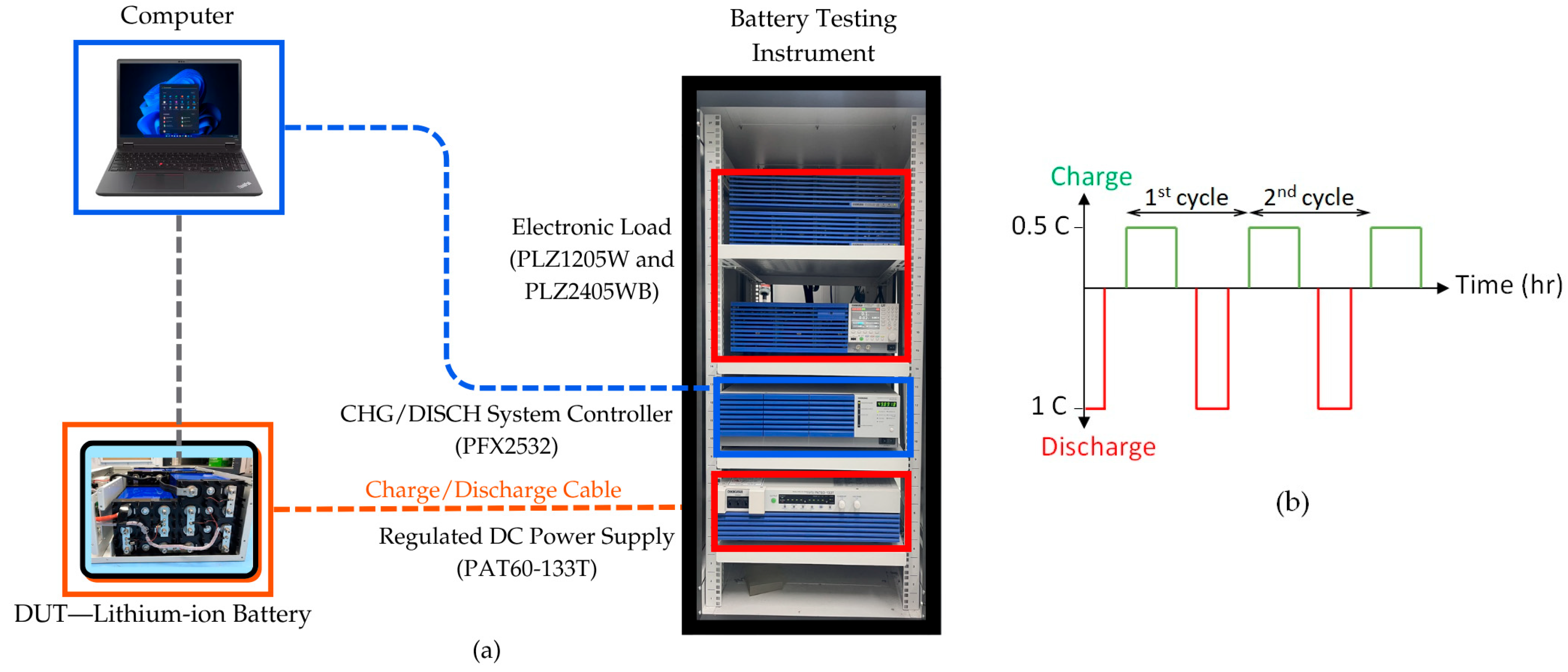
This study examined four packs of 48 V 100 Ah LFP batteries. The batteries were charged with a constant current until the terminal voltage reached the cutoff voltage; then, the batteries were rested for a while to reduce the internal temperature of the battery. The battery was then discharged at a constant current of 100 A (1 C). The discharge operation was terminated once the discharge cutoff voltage was reached. The batteries were rested again before the subsequent charge cycle. All cycling measurements were conducted at a constant room temperature of 25 °C. The BMS was configured to trigger an alarm at 55 °C and to initiate a cutoff at 60 °C. To eliminate the influence of temperature as a variable, the ambient temperature was consistently maintained at 25 °C, and the battery temperature did not exceed 55 °C during any of the tests. Similarly, the LFP battery packs used in this study are intended for stationary communication systems and are housed in temperature-controlled enclosures during real-world operation, ensuring consistency with the laboratory conditions and minimizing the influence of ambient thermal variability. This setup ensures that the analysis focuses solely on non-thermal factors affecting the SOH of the lithium-ion battery. The experimental setup is illustrated in Figure 1a. The charge–discharge testing procedure consists of four steps, as outlined below:

Step1: The compatibility between the device under test (DUT) and the battery testing instruments must first be assessed to ensure proper interaction with the BMS of the lithium-ion battery. If the BMS exhibits abnormal behavior—such as the DUT being unable to charge or discharge using the testing equipment—adjustments must be made by the provider before proceeding to the next step.

Step2: Once the DUT is confirmed to function properly with the battery testing instruments, testing parameters are configured to reflect practical operating conditions. These parameters include charging/discharging currents, voltage limits, and cutoff conditions.

Step3: Prior to full-scale testing, a single charge–discharge cycle is conducted to evaluate the initial condition of the DUT. BMS parameters are set using the BMS programming interface. The criteria for passing the pre-test include the following: (1) the DUT must undergo a discharge at 1 C with a discharge time exceeding one hour, and (2) no alarms or protections must be triggered during the test.

Step4: If the DUT passes the pre-test cycle, it is subjected to a 100-cycle charge–discharge test. During this phase, the DUT is charged at rates ranging from 0.2 C to 1 C, as specified by the manufacturer, and discharged at a constant rate of 1 C. Figure 1b presents a schematic diagram illustrating the conventional charge/discharge switching sequence used in battery testing. The performance degradation of the lithium-ion battery is assessed by comparing the discharge duration of the 1st and the 100th cycle.

Table 1. Items of equipment used in the charge–discharge testing setup and their respective functions.

Equipment Description	Function
Regulated DC Power Supply (PAT60-133T)	Supplies direct current (DC) voltage and current following a constant current–constant voltage (CC–CV) profile for charging the battery.
CHG/DISCH System Controller (PFX2532)	Controls and manages the charging/discharging process and interfaces with other devices.
Electronic Load (PLZ1205W and PLZ2405WB)	Extracts energy from the battery at a constant current during discharging to simulate load.
DUT—Lithium-ion Battery	Stores energy during charging and releases energy during discharging. The battery packs used in this study are as follows: LMU48100 A01 (Pack 1), FHSMARTLi48100 (Pack 2), LFP48-100 (Pack 3), and TBL48100 (Pack 4).
Computer	Monitors and controls the experiment, logs data, and communicates with the controller.

presents the key components of the experimental setup used for lithium-ion battery charge–discharge testing, along with a brief description of each component’s function within the system. The charge and discharge processes were performed repeatedly using a set of parameters summarized in

Table 2. Battery charging and discharging parameters.

LFP Battery	Charge			Discharge			Max. Cycle
	Vcutoff (V)	Current (A)	Rest Time (min)	Vcutoff (V)	Current (A)	Rest Time (min)
Pack 1	52	20 (0.2 C)	30	40	100 (1 C)	30	75
Pack 2	53	20 (0.2 C)	30	39	100 (1 C)	60	100
Pack 3	54	50 (0.5 C)	60	41	100 (1 C)	60	100
Pack 4	52	50 (0.5 C)	90	40	100 (1 C)	90	100

. All batteries were discharged at 1 C, delivering a constant current of 100 A until their voltages reached the specified cutoff values. In contrast, the charging rates varied (0.2 C, 0.5 C) among batteries according to the specifications provided by the manufacturer. The capacity of the battery can be calculated from the Coulomb Counting formula as

$$C={\int }_0^{t}I\left(t\right)dt$$

(1)

To analyze and model the degradation of battery capacity over time, this study investigates four mathematical models, namely, linear, quadratic, single-exponential, and double-exponential models, using MATLAB. The linear and quadratic models provide simple representations of uniform and accelerating degradation trends, respectively. Meanwhile, the single-exponential model captures capacity fade with fast initial drop followed by saturation, and the double-exponential model combines two degradation phases which can offer a more comprehensive fit across different aging stages. The four are expressed as follows:

$$\mathrm{Linear}: C=a_{1}N+a_2$$

(2)

$$\mathrm{Quadratic}: C=b_1{N}^2+b_{2}N+b_3$$

(3)

$$\mathrm{Single-Exponential}: C=c_1{e}^{-c_{2}N}$$

(4)

$$\mathrm{Double-Exponential}: C=d_1{e}^{-d_{2}N}+d_3{e}^{-d_{4}N}$$

(5)

where $C$ denotes the battery capacity, $N$ represents the number of discharge cycles, and $a_i,b_i,c_i,d_i$ are the respective model coefficients.

This work developed and evaluated a modeling approach using lithium iron phosphate (LFP) battery packs. However, two key limitations should be noted. First, the model should be extended and validated across diverse chemistries and configurations, as nonlinear degradation phenomena—such as SEI formation—vary with electrode materials, cell formats, and operating conditions. Second, since the analysis was based on data collected under controlled temperature conditions, future research should evaluate the model’s performance in environments with variable thermal profiles.

3. Results and Discussion

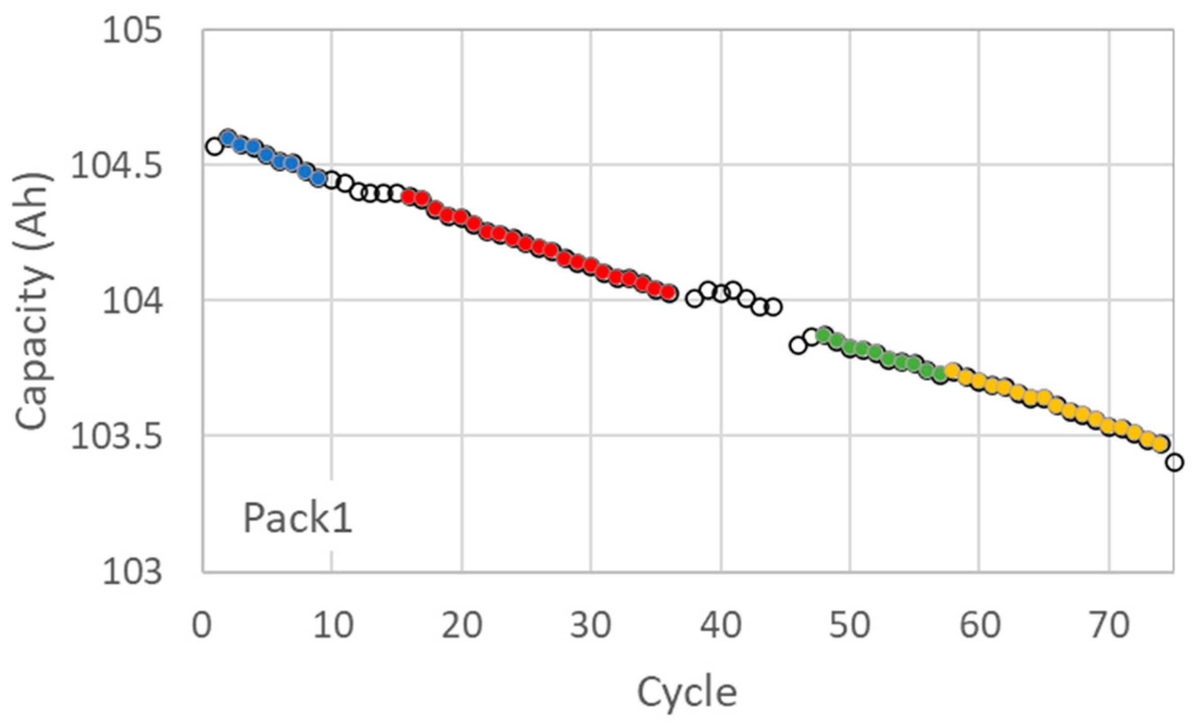
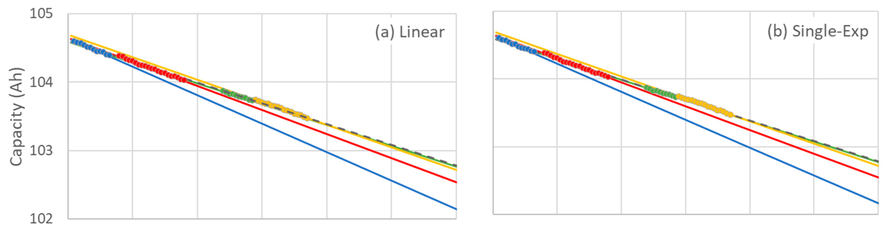
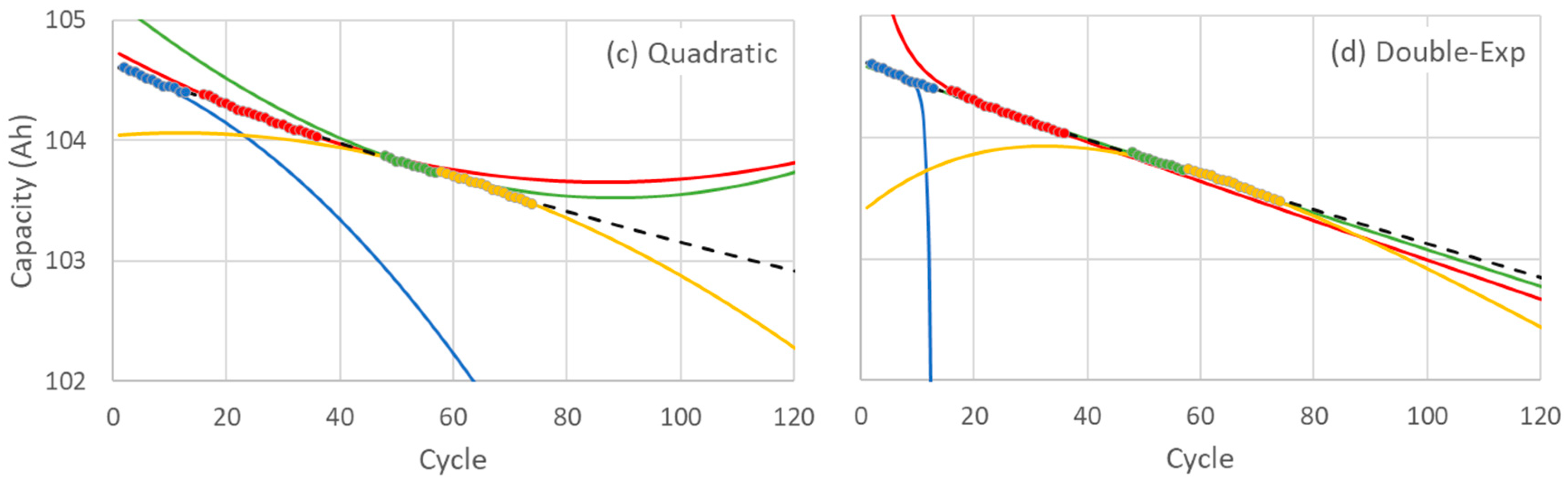
Experimental data, including discharge current, terminal voltage, and temperature, were obtained from the battery testing process. These data were used to estimate battery capacity using the Coulomb Counting method, which integrates the discharge current over time to evaluate capacity fade. Figure 2 presents the capacity degradation profile of the LFP battery pack (Pack 1), in which four distinct datasets (indicated by different colors) are used as inputs for the four predictive models. The linear and single-exponential models produce consistent trendlines across all datasets (Figure 3a,b), whereas the quadratic and double-exponential models exhibit noticeable deviations from the observed degradation behavior (Figure 3c,d). To quantitatively assess model performance, the Akaike Information Criterion (AIC), Bayesian Information Criterion (BIC), and adjusted coefficient of determination (adjusted R²) are computed, as summarized in

Table 3. Akaike Information Criterion (AIC), Bayesian Information Criterion (BIC), and adjusted coefficient of determination (adjusted R²) of the four models evaluated over 100 cycles.

Model	Dataset	AIC	BIC	Adjust R2
Linear	cycles 2–13 (blue)	−112.261	−107.071	0.128
	cycles 16–36 (red)	−141.68	−136.49	0.352
	cycles 48–57 (green)	−148.244	−143.054	0.394
	cycles 58–74 (yellow)	−144.704	−139.514	0.372
Single-Exp	cycles 2–13 (blue)	−113.915	−108.725	0.143
	cycles 16–36 (red)	−142.046	−136.856	0.355
	cycles 48–57 (green)	−148.272	−143.082	0.394
	cycles 58–74 (yellow)	−144.598	−139.408	0.371
Quadratic	cycles 2–13 (blue)	135.463	143.249	−9.541
	cycles 16–36 (red)	−134.751	−126.965	0.312
	cycles 48–57 (green)	−127.330	−119.545	0.259
	cycles 58–74 (yellow)	−130.220	−122.434	0.280
Double-Exp	cycles 2–13 (blue)	2.841 × 104	2.842 × 104	−1.246 × 10125
	cycles 16–36 (red)	−118.777	−108.396	0.199
	cycles 48–57 (green)	−144.272	−133.891	0.381
	cycles 58–74 (yellow)	−96.170	85.790	−0.006

. These values are evaluated over a 100-cycle range. A model with lower AIC and BIC values, and an adjusted R² closer to 1, is considered to provide a better fit. The results indicate that the red, green, and yellow datasets provide better fits when using the linear and single-exponential models. In contrast, the quadratic and double-exponential models exhibit poor fitting performance, with substantial deviations observed at both the initial and later cycle ranges. Notably, the blue curve—corresponding to the dataset comprising the earliest cycle points—shows a rapid decline in the fitted capacities and yields significantly high AIC and BIC values. Although utilizing data from the intermediate cycling stage (red, green, and yellow datasets) improves the fit, as reflected by more favorable AIC, BIC, and adjusted R² values, it also introduces instability at higher cycle counts, as evidenced by the divergence of the fitted curves beyond 100 cycles in Figure 3c,d. This instability limits their applicability for long-term capacity prediction. Consequently, this study focuses subsequent analysis on the linear and single-exponential models due to their robustness and suitability for accurate capacity forecasting using limited cycle data.

3.1. Evaluation of Data Point Requirements for Reliable Linear Capacity Prediction

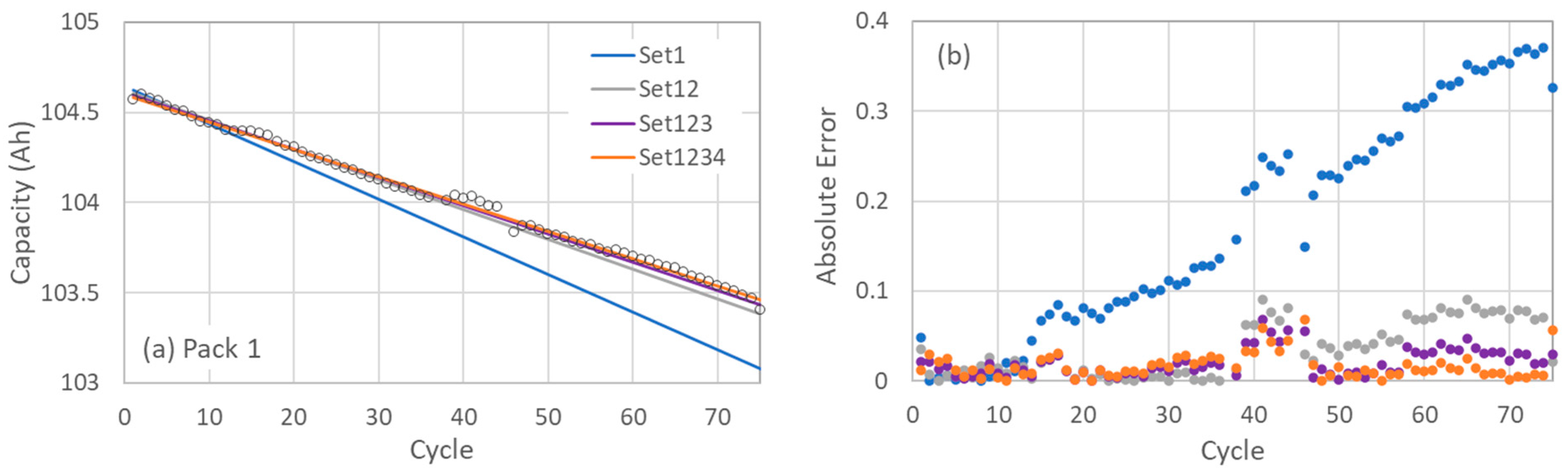
To ensure the reliability of capacity prediction using a linear model, an adequate number of data points must be considered. As illustrated in Figure 2, four distinct datasets were utilized in the modeling process: set1 (blue dots), set2 (red dots), set3 (green dots), and set4 (yellow dots). In this section, the number of points used for linear fitting was progressively increased by combining additional datasets into set1 to assess the effect of data quantity on prediction accuracy. These combined sets are denoted as set12, set123, and set1234 in Figure 4. Set1, which spans cycles 2 to 13, initially demonstrates a satisfactory fit; however, its associated prediction error increases considerably at higher cycle numbers, indicating that data from the first ten cycles alone is insufficient for accurate long-term prediction. As illustrated in Figure 4a, the combined datasets yield improved fits compared to using Set1 alone. The linear fits derived from the combined datasets deviate from the experimental values by less than 0.1 in all cases, as shown in Figure 4b. The prediction errors were quantitatively assessed using the mean absolute error (MAE) and root mean square error (RMSE), defined as

$$MAE={\displaystyle \frac{1}{m}}{\sum }_{i=1}^m\left|y_i-{\widehat{y}}_i\right|$$

(6)

$$RMSE=\sqrt{{\displaystyle \frac{1}{m}}{\sum }_{i=1}^m{\left(y_i-{\widehat{y}}_i\right)}^2}$$

(7)

For set1, the MAE and RMSE values were calculated to be 0.171 and 0.211, respectively. In contrast, the combined set12, which includes 28 data points from the first 36 cycles, yielded significantly reduced MAE and RMSE values of 0.034 and 0.046, respectively. Further improvement was observed with set123 (38 data points from the first 57 cycles) and set1234 (55 data points from the first 74 cycles), achieving MAE (RMSE) values of 0.020 (0.025) and 0.016 (0.021), respectively. These results confirm that increasing the number of data points significantly improves prediction accuracy. Notably, using the first 36 cycles (combined set12) reduces the prediction error by approximately a factor of five compared to set1, indicating that this subset may be sufficient for reliable modeling.

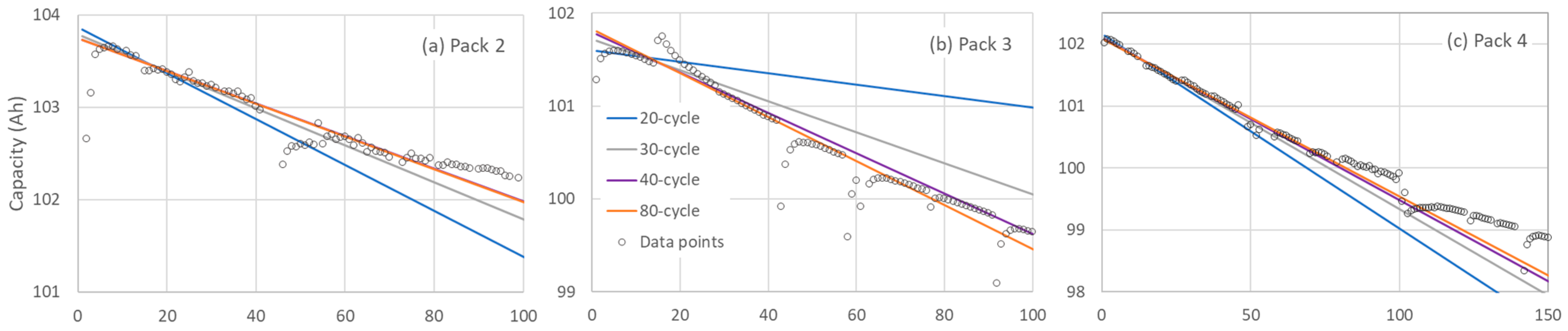
To further investigate the number of data points required for capacity prediction within a 100-cycle aging range, linear fits were performed using the first 20, 30, 40, and 80 cycles in three battery cases (two with 100 cycles and one with 150 cycles). The results, presented in Figure 5 reveal that increasing the number of data points from 20 to 30 cycles substantially reduces the prediction error by half. Additional improvements were noted when using 40 cycles; however, the increase from 40 to 80 cycles did not yield a significant reduction in error. These findings suggest that approximately 30 to 40 discharge cycles are adequate for accurate capacity prediction within the first 100 cycles of battery aging.

3.2. Estimation of Capacity Degradation Slopes Through Curve Fitting

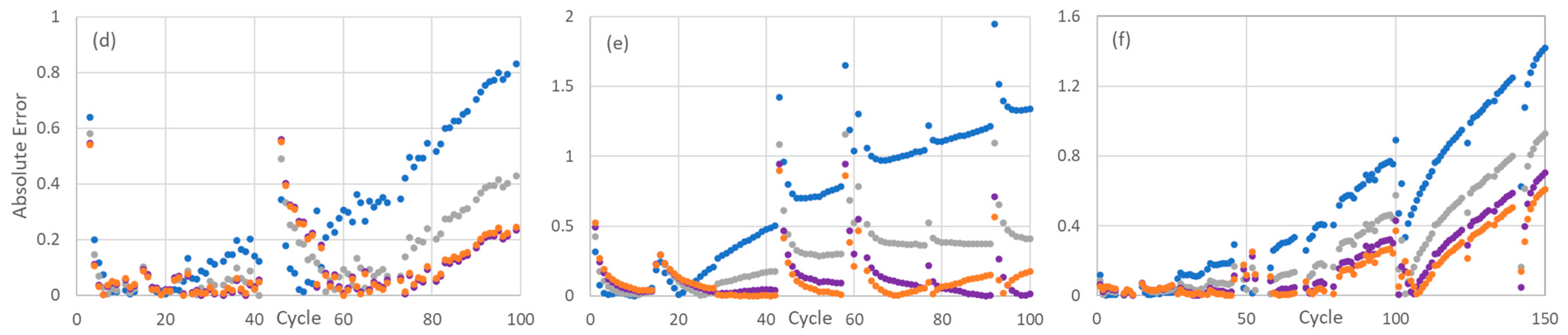
In this section, the nonlinearity of capacity degradation is considered, as a noticeable increase in deviation is observed beyond the 80th cycle. This trend is also reflected in the rising prediction errors shown in Figure 5d–f after the 80th cycle. Although the battery packs were cycled under slightly different charging conditions, all exhibited a similar nonlinear degradation pattern beginning around the 80th cycle, suggesting a consistent underlying aging mechanism. This nonlinear trend may be attributed to electrochemical processes such as SEI growth saturation, the onset of lithium plating, or the progressive loss of active material. These phenomena typically result in a degradation profile characterized by an initial rapid capacity drop, followed by a slower and more stable decline over prolonged cycling [8]. To capture this behavior more accurately, it is appropriate to incorporate an exponential decay term into the linear model, allowing the slope to gradually decrease and reflect the transition from early-stage to long-term degradation. The equation is in the following form:

$$C=e^{-\beta N}{a}_{1}N+a_2$$

(8)

where the term $e^{-\beta N}$ introduces a decreasing slope with the decay rate governed by the parameter $\beta$, capturing a rapid initial decline in capacity followed by a more gradual degradation. However, this modified equation exhibits a turning point at $N=1/\beta$, beyond which the capacity function increases as illustrated in Figure 6, leading to an unphysical prediction. Furthermore, as $e^{-\beta N}$ asymptotically approaches zero for large values of $N$, the capacity function converges to the constant $a_2$. 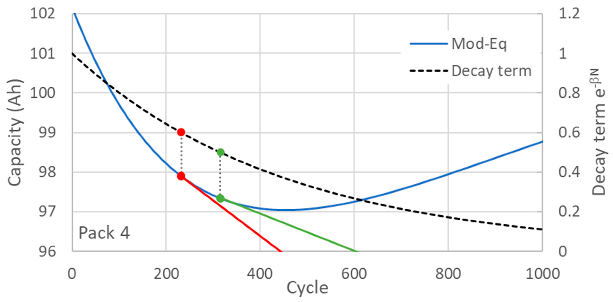To prevent unphysical increases in capacity resulting from slope reversal—i.e., when the exponential term becomes too small—a cutoff cycle is introduced. Beyond this point, the model reverts to a conventional linear decay using the final slope prior to the cutoff (see green and red lines in Figure 6). This hybrid approach ensures physical realism while preserving predictive flexibility. Figure 6 illustrates the behavior of the exponential term and the corresponding capacity function, highlighting the turning point. Specifically, the exponential term $e^{-\beta N}$ reaches the turning point (approximately 0.37) around the 450th cycle, after which the capacity function begins to increase, violating physical expectations. Thus, the cutoff should be selected above this threshold. The selection of the decay rate $\beta$ is also critical, as it directly influences the prediction accuracy of the model. In this study, the value of $\beta$ is chosen to minimize the absolute error between the model predictions and the experimental data.

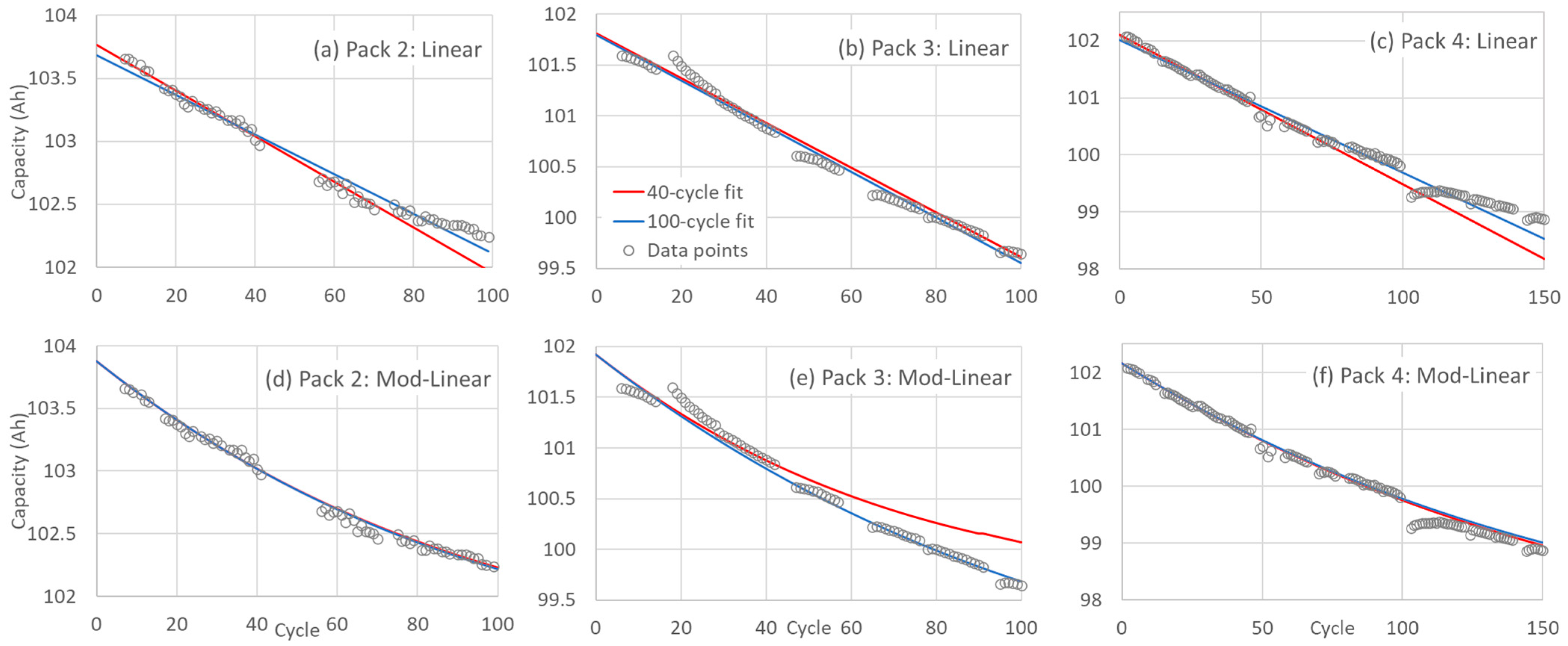
Figure 7 presents the capacity predictions from the linear model (Figure 7a–c) and the modified linear model with a cutoff value of 0.6 (Figure 7d–f). The fits for cutoff values of 0.5 and 0.7 are very similar to the 0.6 case over the 100-cycle range. The single-exponential model is excluded from the figure because its fitting line does not significantly differ from the linear fit in the given range. Two cases are evaluated: a 40-cycle fit (red line) and a 100-cycle fit (blue line). In the 40-cycle case, the first 40 cycles of experimental capacity data are used to fit the linear and single-exponential models. For the modified linear model, two parameters are determined: the initial slope is calculated using the first 20 cycles, and the decay factor $\beta$ is determined using the first 40 cycles. The 100-cycle case follows the same procedure, with the decay factor $\beta$ determined from the first 100 cycles instead. The results indicate that for the linear model, prediction accuracy improves with the 100-cycle dataset.

However, for the modified linear model, increasing the dataset from 40 to 100 cycles does not substantially affect accuracy, as evidenced by the close overlap between the red and blue lines. This suggests that the 40-cycle dataset is sufficient for accurate long-term prediction in most cases. It is noted that abrupt anomalies in the cycling data can significantly affect model performance, particularly in early-stage predictions. For instance, Pack 3 exhibits a sudden increase in capacity at the 18th cycle. Under these conditions, the 40-cycle fit fails to capture the long-term trend, leading to substantially higher errors—more than double the MAE and RMSE compared to the linear and single-exponential models. When the 100-cycle dataset is used, the prediction accuracy improves markedly, with the MAE (RMSE) decreasing from 0.1790 (0.2078) to 0.0666 (0.0844) Ah, as shown in

Table 4. MAE and RMSE of the linear, single-exponential, and modified linear (cutoff = 0.6) models.

LFP Battery	Parameter $\mathit{\beta }$ (Cycle−1)	MAE (Ah)			RMSE (Ah)
		Linear	Single-Exp	Mod-Linear	Linear	Single-Exp	Mod-Linear
The 40-cycle fit
Pack 1	0.0044	0.0239	0.0232	0.0255	0.0298	0.0288	0.0346
Pack 2	0.0044	0.0738	0.0721	0.0336	0.0982	0.0952	0.0394
Pack 3	0.0057	0.0657	0.0676	0.1671	0.0749	0.0768	0.1924
Pack 4	0.0024	0.1994	0.1844	0.0596	0.2707	0.2492	0.0717
The 100-cycle fit
Pack 1	0.0039	0.0280	0.0275	0.0248	0.0309	0.0304	0.0322
Pack 2	0.0043	0.0545	0.0540	0.0328	0.0618	0.0612	0.0374
Pack 3	0.0038	0.0528	0.0525	0.0666	0.0635	0.0634	0.0844
Pack 4	0.0025	0.0921	0.0874	0.0679	0.1198	0.1132	0.0849

. This sensitivity highlights a potential limitation of the model when applied to datasets containing irregular degradation patterns. Incorporating anomaly detection or data pre-processing techniques may help mitigate these effects in future implementations, thereby enhancing the robustness and reliability of long-term forecasting. Additionally, for battery Pack 1, which includes only 75 cycles, all three models yield relatively similar MAE and RMSE values. This is likely because degradation remains nearly linear within this limited range. Thus, the modified linear model does not yield significant advantages under short-cycle conditions.

3.3. Cycle Life Prediction Based on Degradation Models

From Table 4, the performance of the linear and single-exponential models is compared with that of the proposed modified linear model over a 100-cycle test range. The extension of testing to 150 cycles for Pack 4 further highlights the suitability of the modified linear model in capturing nonlinear degradation behavior over extended cycling.

Table 5. MAE comparison between proposed models (40-cycle fits) and data-driven models from Refs. [29,30].

Literature	Model	Average MAE (Ah)	Description	Advantages
Ref. [29]	LSTM	0.0050	Processes time-series data capturing temporal dependencies.	Effective for tracking degradation over cycles.
	CNN	0.0061	Convolutional neural network capturing localized features.	Simple and efficient; originally designed for image data.
	MSCNN	0.0034	Uses varied kernel sizes to extract multi-scale features.	Captures complex, nonlinear degradation patterns effectively.
Ref. [30]	LSTM	0.0303	Processes time-series data capturing temporal dependencies.	Effective for tracking degradation over cycles.
	ALSTM	0.0121	LSTM enhanced with attention mechanism.	Focuses on important time steps, improving accuracy.
	HI-LSTM	0.0405	LSTM with an explicit health index input.	Adds interpretability through physically meaningful HI.
	HI-ALSTM	0.0103	Combines attention and health index.	Achieves highest prediction accuracy and robustness.
Our work	Linear	0.0907	Assumes uniform capacity fade over cycles.	Simple and effective for early-cycle predictions with limited data.
	Single-Exp	0.0868	Models fast initial drop and slow stabilization in degradation.	Improves short-term prediction with slight added complexity.
	Mod-Linear	0.0715	Linear model with exponentially decaying slope and cutoff.	Captures nonlinear behavior; robust long-term predictions using limited data.

summarizes the key characteristics, modeling approaches, and advantages of both empirical and data-driven models for SOH prediction of lithium-ion batteries. Among data-driven methods, CNN and MS-CNN extract spatial and multi-scale features from raw signals, enhancing the modeling of complex degradation. LSTM captures temporal dependencies in cycle data, while ALSTM, HI-LSTM, and HI-ALSTM improve upon LSTM by incorporating attention mechanisms and health indices to emphasize relevant features and add physical interpretability. The modified linear model, which incorporates a continuously decaying slope through an exponential function, was found to yield a MAE slightly higher than that of advanced machine learning methods. While data-driven models generally provide superior accuracy, empirical approaches—particularly the modified linear model—offer greater practicality in scenarios where data availability or computational resources are constrained.

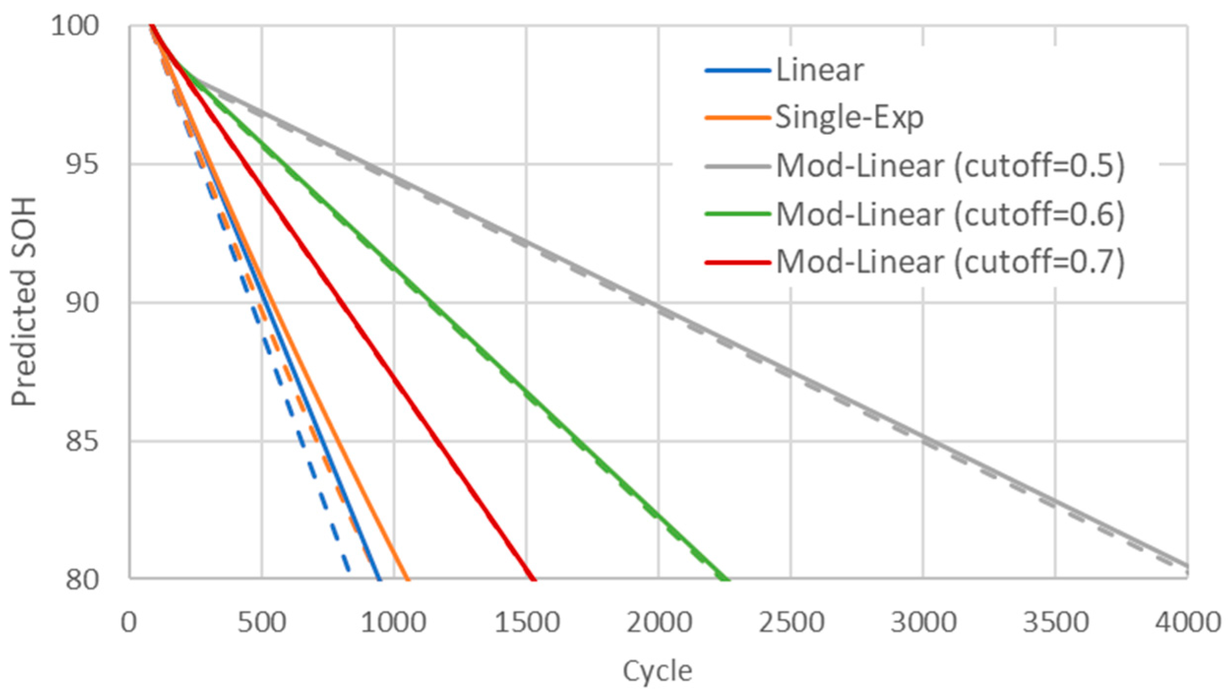
To assess long-term prediction capability, the SOH forecast is extended to 5000 cycles, thereby revealing the limitations of the linear and single-exponential models in accurately modeling capacity degradation. In general, the EOL is considered to occur when the battery retains only 80% of its initial capacity. In this study, SOH is calculated using the Coulomb Counting method, defined as

$$SOH={\displaystyle \frac{C_c}{C_0}}\times 100\%$$

(9)

where $C_c$ is the current capacity and $C_0$ is the initial capacity. The predicted SOH values derived from the linear, single-exponential, and modified linear models are illustrated in Figure 8, while the corresponding EOL predictions are summarized in

Table 6. End of battery life (SOH = 80%) predicted from the linear, single-exponential, and modified linear equations.

LFP Battery	Linear (Cycle)	Single-Exp (Cycle)	Mod-Linear (Cutoff = 0.7) (Cycle)	Mod-Linear (Cutoff = 0.6) (Cycle)	Mod-Linear (Cutoff = 0.5) (Cycle)
Pack 1	1317/1489	1465/1649	2280/2265	3447/3395	6429/6364
Pack 2	1147/1319	1274/1459	1768/1750	2660/2634	4933/4954
Pack 3	927/910	1030/1004	1351/1330	2033/1988	3802/3659
Pack 4	780/878	865/967	1402/1405	2051/2066	3691/3737

Note: Values in the format X/Y indicate EOL from the 40-cycle (X) and 100-cycle (Y) fits.

, providing further insights into model performance across different data quantities and battery packs. To examine the influence of the cutoff on model performance, cutoff values of 0.5, 0.6, and 0.7 were selected for analysis. These values were chosen to ensure that the cutoff occurred prior to the turning point of the exponential decay term, thereby maintaining physical plausibility while allowing assessment of the model’s sensitivity to the cutoff position. The results indicate that the modified linear model with the cutoff values of 0.5, 0.6, and 0.7 yields similar SOH predictions for both 40-cycle and 100-cycle fits, demonstrating greater robustness when data are limited. The linear and single-exponential models exhibit a more rapid decline in SOH, whereas the modified linear model reflects a slower degradation trend. Lower cutoff values result in slower predicted degradation. According to typical LFP battery specifications, the cycle life at 80% SOH is generally in the range of 2000–4000 cycles [32], depending on factors such as cycling depth, temperature, and charging strategy. Therefore, the EOL predictions from the linear and single-exponential models—nearly twice as early as those from the modified linear model—can be considered underestimations of the actual cycle life. In contrast, the modified linear model with a 0.5 cutoff value slightly overestimates battery life in the case of Pack 1 and Pack 2. Overall, cutoff values between 0.5 and 0.7 in the modified linear model provide reliable SOH and EOL predictions, making them suitable when early-cycle data are limited.

4. Conclusions

This work proposes and evaluates empirical mathematical models for the prediction of lithium-ion battery capacity degradation and SOH estimation. Through controlled experiments on four LFP battery packs, the linear and single-exponential models were found to provide reliable short-term capacity predictions over 100 cycles. The results show that data from the first 30 cycles are sufficient to achieve acceptable prediction accuracy, and extending the dataset to 40 cycles reduces the MAE and RMSE by approximately 50%. However, a notable nonlinearity in the degradation trend emerges beyond 80 cycles, as the rate of capacity fade slows significantly. To better capture this behavior, a modified linear model was introduced, incorporating an exponential decay term in the slope with an appropriate cutoff strategy. Comparative analysis of 40-cycle and 100-cycle fits reveals that the modified linear model offers consistent and stable predictions, even in long-term forecasts. In contrast, although the accuracy of the linear and single-exponential models improves with a larger dataset, they fail to capture the nonlinear degradation observed at extended cycle counts. This limitation is most evident in Pack 4, which exhibits the highest MAE and RMSE values among all tested packs—0.1994 (0.1844) and 0.2707 (0.2492), respectively, for the linear (single-exponential) model using a 40-cycle fit. Consequently, the predicted EOL is 780 cycles for the linear model and 865 cycles for the single-exponential model, both of which underestimate the expected cycle life of approximately 2000–4000 cycles as specified by the manufacturer. Even when using a 100-cycle fit, the predicted EOL remains below the specification range, a trend that is similarly observed in Packs 1–3. These findings highlight the importance of selecting an appropriate degradation model and cutoff parameter, especially for long-term SOH and EOL forecasting in BMS. Accurate predictions are essential for optimizing charging strategies, ensuring operational reliability, and avoiding premature battery replacement or unexpected failures.