Abstract
With the large-scale integration of new power systems and distributed generators (DGs), cable fault detection and localization face numerous challenges, where artificial intelligence (AI) techniques demonstrate significant advantages. This review first outlines the causes of cable faults and traditional methods for fault detection and localization. Subsequently, it comprehensively analyzes the applications of both conventional machine learning and deep learning approaches in this field, elaborating on their application scenarios, strengths, defects, and successful case studies, providing valuable references for researchers and professionals. Additionally, the paper discusses the strengths and limitations of current AI techniques, along with the impacts introduced by DG integration. Finally, it highlights future development trends and potential research directions for advancing AI-based solutions in cable fault detection and localization.
1. Introduction
In the future, countries around the world must fully implement the new development philosophy and accelerate the construction of a new-type power system. This involves actions such as optimizing and strengthening the main grid framework, increasing the proportion of new energy electricity in transmission channels, and developing system-friendly new energy stations. Additionally, the continuous development of new infrastructure projects—including 5G technology, artificial intelligence (AI) combined with the Internet of Things (IoT), and big data integrated with AI—aims to meet requirements such as high-speed transmission, memory expansion, high power density, and high stability in power systems. These efforts require stable and efficient power transmission [1,2,3]. As shown in Figure 1, the distribution network plays a critical role in the overall performance of power systems by receiving electricity from the grid and transmitting and distributing it to consumers.
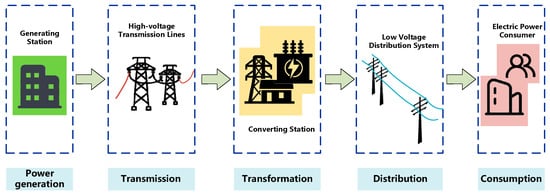
Figure 1.
Power system structure.
Cables, as a critical component of urban distribution networks, have been widely adopted during the urbanization process. However, due to the current concentration of cable installations in urban core areas, numerous medium- and low-voltage cables, as well as some high-voltage cables, are deeply buried underground in tunnels, as shown in Figure 2. The internal environment of cable trenches is complex and riddled with hidden dangers, which significantly compromise cable installation quality and operational effectiveness, potentially leading to cable operation accidents such as partial discharge and flashover faults. These early-stage faults are characterized by a short duration and recurrence, making them prone to evolve into permanent failures. Some cable lines have experienced overload conditions or excessive fault currents, even resulting in thermal breakdown and electric arcs that ultimately lead to cable fires. Cable operation faults not only cause substantial economic losses but also endanger personal safety and damage the social reputation of power companies. This situation poses severe challenges for grid system operation and maintenance departments.
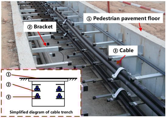
Figure 2.
Schematic diagram of cable trench.
Taking China as an example, its rapidly evolving power grid system has integrated numerous renewable energy sources, such as photovoltaic power generation, wind power, hydropower, and biomass power generation, with renewable electricity production steadily increasing, as illustrated in Figure 3. Data from the National Energy Administration of China indicates that by December 2024, the national renewable energy power generation reached 3.46 trillion kWh, representing an increase of 541.9 billion kWh compared to the same period last year, accounting for approximately 86% of the total incremental electricity consumption in society. The principles of renewable energy power generation and the composition of operational control methods differ significantly from traditional power systems, leading to distinct fault characteristics that make fault analysis in the new grid system increasingly complex. Under these circumstances, traditional approaches for cable fault detection and location have demonstrated certain limitations, including difficulties in data processing, high manual workload, and slow response times. In recent years, with rapid advancements in computer technology, artificial intelligence (AI) methods have been applied to the field of cable fault detection and localization, effectively addressing the challenges faced by conventional techniques. As a crucial branch of artificial intelligence, deep learning [4] focuses on constructing deep neural network models to automatically learn hierarchical feature representations from massive datasets. This approach, extended from artificial neural network architectures, employs multilayer nonlinear transformations to model intrinsic data patterns. Through activation functions and gradient descent algorithms, these models can progressively optimize their parameter spaces, achieving superior performance in tasks such as image recognition [5], natural language processing [6], and speech analysis [7]. Some researchers have applied deep learning techniques to cable fault detection and localization, aiming to leverage their capabilities in handling the vast data volumes of next-generation power systems. These methods have already demonstrated unparalleled advantages in terms of accuracy, speed, and adaptability compared to traditional approaches.
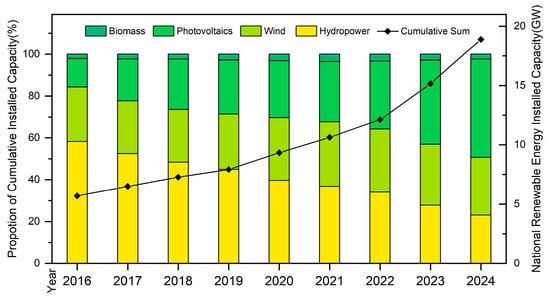
Figure 3.
Chart of China’s cumulative installed capacity of renewable energy power generation (2016–2024).
Based on the above content, this paper presents a comprehensive review of cable fault identification. The research contributions include (a) surveying the latest research status of cable fault identification and location methods in distribution networks; (b) providing a detailed review of the application of machine learning, particularly the latest deep learning algorithms, in cable fault detection and location; and (c) analyzing and comparing relevant techniques to clarify research trends and limitations. Compared to previous studies, this work places greater emphasis on the application of diverse deep learning models for cable fault detection and localization.
This paper comprehensively analyzes existing methods for cable fault detection and localization, with the organizational structure outlined as follows: Section 2 introduces the causes of cable failures. Section 3 presents conventional approaches for cable fault detection and localization. Section 4 and Section 5 systematically review the applications of traditional machine learning and deep learning techniques in cable fault detection, identification, and localization, respectively, while evaluating their effectiveness and accuracy. Section 6 systematically reviews the advantages and limitations of artificial intelligence methods in related fields and discusses the impact of distributed generation (DG) integration on fault analysis. Finally, Section 7 provides a summary and outlook for future research directions in this domain.
2. Analysis of Cable Fault Causes
After installation and operation, power cables are subjected to comprehensive impacts from electrical, thermal, mechanical, and environmental factors, leading to insulation aging, reduced operational reliability, and severe cases of breakdown accidents. Based on influencing environmental factors, fault causes can be categorized into three types: local overheating, insulation moisture, and mechanical damage.
2.1. Local Overheating
During cable operation, localized overheating represents one of the most common fault triggers, primarily manifesting as abnormal temperature elevation in specific cable regions beyond material endurance limits, which subsequently causes insulation performance deterioration or conductor melting. According to IEC 60502-1:2004 standards [8], the long-term maximum operating temperature for cross-linked polyethylene (XLPE) insulation is 90 °C. When cables continuously operate above their rated current capacity, Joule heating generated by conductor resistance significantly intensifies, accelerating thermal aging of insulation layers. Research [9] has demonstrated that breakdown strength rapidly declines during initial thermal aging stages—after 48 h of thermal aging at 160 °C, the breakdown voltage decreases from 80.48 kV/mm to 74.15 kV/mm. From a microstructural perspective, thermal aging disrupts the crystalline structure of XLPE, increasing the number of interfaces between crystalline and amorphous regions, thereby inducing structural damage and dielectric performance degradation [10]. Additionally, when an increase in contact resistance occurs at cable joints or terminations due to issues such as oxidation or loosening, local hot spots will form in the insulation layer. Certain installation environment problems—such as ruptured hot water pipes near cables, water accumulation in cable trenches, poor ventilation, or dense cable arrangements—can also impede heat dissipation, causing heat accumulation. These ultimately lead to the insulation degradation of the cables.
2.2. Insulation Moisture
Moisture ingress in cables primarily results from inadequate sealing at cable ends during installation and physical damage caused by external forces, leading to water penetration. Insulation moisture infiltration can significantly reduce dielectric strength, serving as a critical factor in cable breakdown failures. When external sheath cracks develop due to mechanical damage or material aging, moisture gradually penetrates longitudinally through ports or defects into the insulation layer. This process occurs slowly without immediate fault manifestation, but prolonged moisture exposure exacerbates aging progression and induces water tree discharges, eventually resulting in insulation breakdown. The breakdown experiments [11] demonstrate that moisture-affected XLPE samples exhibit breakdown voltages reduced to between 85% and 94% of normal conditions.
2.3. Mechanical Damage
Mechanical stress directly compromises cable structural integrity by forming microvoids that can trigger partial discharges and treeing structures, ultimately leading to operational failures. Typically, mechanical damage originates from excessive traction forces or insufficient bending radius during installation, which may cause metal shield layer fractures or insulation wrinkles, disrupting the aggregated structure of insulation materials. External pressures such as road construction activities and geological subsidence can further induce compression deformation, resulting in conductor eccentricity or uneven insulation thickness. Animal activities, such as gnawing by rodents or bioerosion by marine organisms, may also cause sheath damage, subsequently leading to compromised structural integrity. Accelerated mechanical aging tests on XLPE/CSPE insulation [12] reveal that cable insulation hardness increases progressively with aging, indicating the severe degradation of insulation and sheath materials due to cross-linking, dehydrochlorination, and oxidation processes. Afia et al. [13] compared Shore D hardness variations between thermally aged and thermo-mechanically aged samples, finding that mechanical stress significantly elevates cable hardness beyond pure thermal stress effects, thereby constituting a primary contributor to polymer material degradation in cables.
3. Traditional Cable Fault Detection and Localization Methods
In distribution network management, the effective implementation of timely preventive maintenance strategies enables the early detection and localization of incipient cable faults, thereby delivering significant operational advantages to utility companies and reducing societal losses. From the utility perspective, the proactive monitoring and diagnosis of potential cable defects can substantially decrease the probability of unexpected failures, enhancing power supply reliability and consumer satisfaction. From a safety standpoint, early fault detection reduces electrical accident risks caused by insulation aging, partial discharges, or short circuits, thus ensuring personnel and public safety during cable operations. Conventional fault detection methods primarily analyze electrical quantities such as traveling waves, grounding currents, and zero-sequence currents in time or frequency domains, deriving diagnostic conclusions through corresponding calculations and comparisons of these parameters.
3.1. Traditional Cable Fault Detection Methods
When transmission lines experience faults, power systems must detect failures to clear them before they escalate system damage. Early engineering applications of cable fault detection were based on electrical characteristics, characterized by rapid computation speed and high efficiency. One of the most common fault detection methods employs the traveling wave principle [14]. Al Hassan et al. [15] proposed a terminal surge arrival detection method using a wave propagation decoupling approach for high-voltage direct current voltage source converter (HVDC-VSC) systems, establishing an equivalent cable model in PSCAD/EMTDC to validate algorithm accuracy. In 2022, Verrax et al. [16] proposed a model to describe grid transient behavior based on previous work. This model employs a simplified traveling wave description to characterize the physical properties of power grids, comprehensively incorporating the effects of soil resistivity and cable shield resistance on the physical model to establish a voltage evolution model for traveling wave propagation across different line segments. Shi et al. [17] introduced a novel method for assessing the health status of individual distribution feeders by integrating power-frequency electrical information and traveling wave information. They argue that when insulation degradation occurs in distribution network cable feeders, the power-frequency signals will remain identical to those of healthy feeders, while traveling waves will emerge in the distribution system. A portable partial discharge (PD) detection and localization system for online insulation condition assessment of inter-array cables in wind farms was proposed in 2023 [18]. This system implements an improved double-ended traveling wave PD detection methodology, which incorporates a pulse-based bidirectional interaction process to enable GPS-triggered pulse synchronization and propagation velocity estimation while eliminating synchronization errors. Table 1 presents a detailed comparison between the developed system and widely adopted offline PD measurement systems, demonstrating the advantages of the new system in portability, time efficiency, labor cost reduction, and improved cost-effectiveness.

Table 1.
Comparison of the development system and the commercial offline PD measurement systems.
With the rapid advancement of signal processing and wireless communication technologies, a new power system concept—the smart grid—has emerged. ZigBee technology is commonly employed to enhance the reliability and stability of intelligent distribution systems. Rajpoot et al. [19] proposed the SUGPDS model, which integrates ZigBee technology with a detection-isolation algorithm for identifying and classifying various underground power cable faults. The identification workflow follows the process illustrated in Figure 4. Experimental results demonstrate the system’s excellent detection and recognition capabilities for open-circuit faults, short-circuit faults, and ground faults in power cables. In 2022, Peng et al. [20] introduced a novel fault-awareness algorithm implemented at edge nodes, which utilizes only the grounding line current from the local terminal of the cable to achieve rapid and reliable fault detection. Compared with [21,22,23], this method requires only grounding line current acquisition with a minimum sampling rate of 3.2 kHz, making it more convenient for measurement. A modal signal decoupling algorithm has been further developed to establish a fault cable identification criterion for MVdc distribution cables. RTDS experiments validate that this approach achieves a fault detection accuracy as high as 99% while maintaining applicability to arc faults.
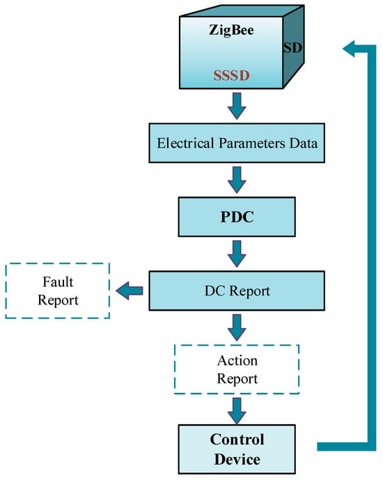
Figure 4.
Flowchart of the process followed by SUGPDS.
However, due to the precision and sensitivity of electrical measurement instruments being affected by on-site interferences, achieving ideal diagnostic performance remains challenging. Many researchers have focused on cable fault detection through equivalent cable modeling and analysis of fault currents, voltages, and impedance spectra. Samet et al. [24] established a fault detection method based on an arc model, which employs similarity analysis of voltage signals combined with cross-correlation function (CCF) and sinusoidal curve fitting. This two-phase approach detects incipient faults while being capable of effectively distinguishing capacitor switching, load variations, and other similar events. According to Table 2, the proposed method maintains a detection accuracy exceeding 98% across various arc fault models. Zhang et al. [25] constructed an electrical model incorporating electromagnetic coupling effects between multiple conductors and photovoltaic (PV) integration, introducing a fault section identification method based on amplitude and polarity feature differences in grounding wire current (GWC) at the source end. This approach achieves identification accuracy approaching 100% while remaining largely unaffected by three-phase imbalance, measurement errors, or cable parameter variations. Building upon this, Zhang et al. [26] established a field-circuit equivalent cable model that comprehensively accounts for multi-conductor electromagnetic coupling impacts on GWC. They proposed a fault detection methodology leveraging periodic variations in GWC frequency components. Fault simulations demonstrate that the amplitude difference in GWC between low and high PV penetration scenarios remains within 10%, with a 98% fault detection rate observed even under 20 dB white noise interference, confirming the method’s strong robustness. Both references [25,26] reveal that GWC exhibits immunity to transient disturbances, noise interference, and fault condition variations, highlighting the broad application potential of GWC-based fault detection in future three-core cable engineering.
Table 2.
The results of the proposed approach in the detection of incipient faults by different arc models and similar events.
3.2. Traditional Cable Fault Location Methods
Cable fault location serves as a critical technique in the power industry, enabling the rapid and accurate identification of fault locations within cables for timely maintenance and ensuring normal power system operation. Traveling wave methods represent one of the most established distance measurement theories, with recent advancements proposed by multiple researchers. Deng et al. [27] introduced a novel traveling wave representation in a 3D subspace, which establishes a direct correspondence between fault locations and complete waveform characteristics from single-terminal measurements. This approach supports a fault location algorithm based on single-ended traveling waves. The algorithm’s workflow, as shown in Figure 5, comprises two stages: offline and online processing. Simulations demonstrate their low sampling frequency requirement (as low as 50 kHz) while maintaining high sensitivity under this sampling rate. Rezaei et al. [28] proposed an alternative single-ended traveling wave fault location algorithm that determines wave arrival times through angle analysis of fitted linear segments. Their simulations across various fault scenarios achieve absolute error margins below 0.086. Compared with HHT and WT-db4-Sc2 methods, the proposed algorithm demonstrates superior performance when fault inception angles (FIA) are small. Double-ended traveling wave ranging shows reduced sensitivity to system operating conditions and thus provides more reliable location results than single-ended approaches. An optimized dual-ended traveling wave fault location solution [29] employs the discrete wavelet transform (DWT) to detect transient traveling wave fronts. Through simulations under various fault conditions, this model demonstrates rapid fault detection and localization within 0.01 s. In the same year, Xie et al. [30] developed an improved dual-terminal fault location algorithm that applies extreme-point symmetric mode decomposition-Teager energy operator (ESMD-TEO) to initial fault traveling wave signals, achieving enhanced robustness against wave velocity variations and line parameter uncertainties. Huang et al. [31] incorporated modal decomposition and the Hilbert–Huang transform to improve the location accuracy of dual-ended traveling wave methods. Simulations demonstrated that this approach enables the precise localization of tree flash faults with absolute error margins below 0.116 per kilometer.
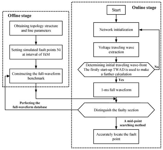
Figure 5.
Fault location algorithm flowchart.
Applying signal processing techniques for filtering, denoising, and feature extraction of fault data can provide enhanced fault-characterizing characteristics for an accurate fault location. Hasanvand et al. [32] compared the fault location accuracy of S-transform and continuous wavelet transform (CWT) in hybrid distribution networks combining overhead lines and cables. The simulation results demonstrated that the S-transform achieves higher-frequency resolution accuracy and greater robustness in fault location applications. Chen et al. [33] employed empirical wavelet transform (EWT) combined with multi-resolution singular value decomposition (MRSVD) to denoise sheath current traveling waves, determining the faulted section through instantaneous polarity analysis of detected traveling waves at each measurement point. However, this method heavily relies on high-frequency current transformers (HFCT), resulting in significant initial investment costs. In frequency domain approaches, Cifuentes et al. [34] utilized an offline system to identify transient mid-frequency responses of fault systems, followed by fault location in online systems through fast Fourier transform (FFT), with the specific methodology illustrated in Figure 6. This method maintained location errors below 3.3% across diverse simulation scenarios. Song et al. [35] introduced numerical Laplace transform (NLT) to establish bidirectional equivalence between frequency-domain analytical solutions and time-domain transient waveforms by incorporating real components of complex frequencies, enabling precise calculation of voltage distribution along cables for accurate fault location. The maximum location error in simulations reached 0.6%, demonstrating superior positioning accuracy. Time-domain fault location research remains relatively limited, exemplified by Bretas et al. [36], who developed a time-domain system model for early-stage single-phase ground faults in underground shielded cables, transforming the problem into linear equations solved by non-negative weighted least squares estimators (NNWLSE) to determine unknown parameters and estimate fault distances.
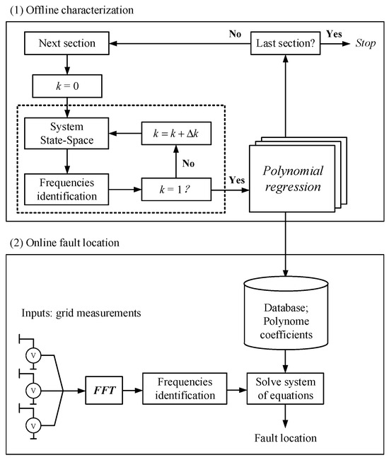
Figure 6.
Schematic diagram of a novel cable fault location method based on transient medium-frequency response.
The aforementioned literature represents established fault location methodologies characterized by straightforward implementation and simple operation, with many approaches already implemented in practical power systems engineering. These techniques typically employ signal processing for sample signal conditioning or rely on modeling-based calculations, thereby achieving significantly reduced implementation costs and low maintenance requirements, which collectively favor their adoption in engineering practices.
3.3. Limitations of Traditional Methods
The methodologies in the aforementioned literature primarily rely on traveling wave techniques, time-frequency domain analysis, and sensor measurements, with some approaches incorporating equivalent modeling of power cables while comprehensively considering multiple critical operational factors. However, as power grid systems grow increasingly large-scale, precise modeling becomes progressively challenging. The massive integration of distributed power sources exacerbates uncertainties and nonlinearities in monitoring data, further amplifying the limitations of these conventional methods. These limitations manifest in three key aspects, as outlined in the following subsections.
3.3.1. Modeling Challenges and Accuracy Issues
With the expanding scale of power grids, complex distribution networks exhibit multiple line branches and intricate topologies, significantly increasing the difficulty of accurate modeling. Traditional methods struggle to precisely characterize line parameters and electrical properties that reflect real-world conditions, leading to deviations in fault detection and location estimation.
3.3.2. Insufficient Data Processing Capability
The integration of distributed power sources intensifies data uncertainties and nonlinearities. Conventional methods face challenges in extracting fault features from monitoring data containing abundant harmonics and fluctuations, compromising location accuracy. Additionally, the massive data volume in large-scale grids may exceed the computational efficiency of traditional techniques, failing to meet real-time requirements and prolonging fault location times.
3.3.3. Limited Adaptability
Traditional approaches are often built upon specific assumptions and conditions, exhibiting poor adaptability when grid structures or operational modes change. Following grid expansion and distributed power integration, operational scenarios become more complex and dynamic. These methods may struggle to automatically adjust to new conditions or require manual recalibration, substantially reducing their universal applicability.
The aforementioned limitations predominantly impact the accuracy of fault detection/localization, computational efficiency, and robustness, necessitating further improvements.
4. Cable Fault Detection and Localization Methods Based on Traditional Machine Learning
With the growing demand for data in power systems, the requirements for efficiency in data processing and analysis have become increasingly higher, leading to the application of a series of machine learning algorithms in cable fault detection and localization methods. Machine learning algorithms primarily refer to the steps and procedures that solve optimization problems through mathematical and statistical approaches. To address different cable model requirements, appropriate machine learning algorithms can be selected to overcome the limitations of traditional methods, which struggle with handling large volumes of data and adapting to the complexities of modern power grids.
4.1. Application of Traditional Machine Learning in Cable Fault Detection
4.1.1. Multilayer Neural Pattern Recognition Algorithms
Multilayer Neural Pattern Recognition Algorithms are inspired by biological neural networks, processing input data through a multi-layered node structure. The input layer receives raw features, while hidden layers perform nonlinear transformations via weight matrices, progressively extracting abstract features. The output layer generates classification or prediction results. During training, the backpropagation algorithm computes gradients based on loss functions, iteratively updating weights to minimize errors. Their core strength lies in hierarchical feature extraction: lower-level neurons identify simple patterns while higher layers integrate complex features. Ledesma et al. [37] proposed a high-impedance fault identification method for distribution networks based on a two-level neural network and synchronous measurements, effectively addressing fault identification challenges in complex distribution network environments while considering issues like DG integration and network reconfiguration. The simulation results show that the trained ANN achieves an accuracy rate of no less than 97.6% for fault identification when network reconfiguration, high-impedance faults, and DG integrations are simultaneously considered. In 2023, Gogula et al. [38] proposed a fault detection method for high-impedance faults by integrating the DWT and Neural Network with Radial Basis Function (NNRBF) algorithm. This method employs DWT to decompose fault currents and extract corresponding eigenvalues, which are then used as inputs for NNRBF. Simulation tests across varying fault resistances demonstrated a detection accuracy of up to 100% for this approach. Bindi et al. [39] developed a predictive method for preventing catastrophic failures in medium-voltage underground cables using Power Line Communication (PLC) technology and an MLMVN-based neural classifier. This method is capable of detecting cable overheating issues. It achieves a fault classification accuracy of 96.03% within the frequency range of 95–450 kHz, and maintains a classification accuracy of over 80% even when the signal-to-noise ratio (SNR) of white noise reached approximately 23 dB.
4.1.2. Support Vector Machine
The Support Vector Machine (SVM) [40] is a supervised machine learning algorithm whose core principle is to find a hyperplane in the feature space that maximizes the margin between samples of different classes, satisfying the following constraint conditions:
where ω represents the weight vector, b denotes the bias, represents the slack variable, and C signifies the regularization function. For linearly separable data, the optimal hyperplane resides precisely at the midpoint of the margin boundaries between the two classes of samples. The sample points lying on these boundaries are termed support vectors. For nonlinear problems, a kernel function K(x, xi) is employed to map the input space into a high-dimensional feature space, rendering the data linearly separable in this new space. Linear SVM is then applied for classification. The final decision function is given by:
In this equation, αi represents the Lagrange multipliers. The objective of SVM training is to solve a convex optimization problem that minimizes the sum of structural risk and empirical risk. In cable fault identification, SVM is commonly used to process feature vectors extracted from cable monitoring data, such as time-domain statistical quantities and frequency-domain energy distributions. The kernel function is selected based on a comprehensive consideration of computational efficiency and the degree of feature nonlinearity, enabling SVM to distinguish between normal operating states and various fault types.
Abu-Rub et al. [41] applied the SVM algorithm to analyze PD signal patterns, enabling the identification and classification of internal insulation defects in cables, thereby improving fault detection accuracy. This method achieves a defect identification accuracy of up to 95.8% and a classification accuracy exceeding 92% for single internal defects, validating SVM’s promising application prospects in cable fault detection. Saad et al. [42] proposed an improved SVM-based fault diagnosis method for medium-voltage cables, utilizing a multi-class support vector machine (MCSVM) in the fractional Fourier domain. The specific algorithm workflow, illustrated in Figure 7, employs one-versus-one (OVO) SVMs to generate all possible pairwise classifiers, effectively reducing computational complexity. The simulation results show this approach achieved a fault detection accuracy of 99.8% with an execution time as low as 0.01 s, outperforming other algorithms such as kNN, PNN, and MLP. Regarding intermittent grounding faults in medium-voltage (MV) distribution networks, Razmi et al. [43] applied five algorithms—SVM, DT, LSTM, RNN, and MLP—for fault classification. As shown in Table 3, SVM demonstrates exceptional performance with an accuracy of 98.9% during the testing phase, proving its effectiveness in handling high-dimensional nonlinear data.
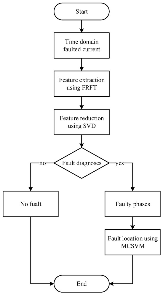
Figure 7.
Flowchart of the proposed method.
Table 3.
Supervised algorithm performance.
4.1.3. Adaptive Neuro-Fuzzy Inference System
The Adaptive Neuro-Fuzzy Inference System (ANFIS) integrates the adaptive learning ability of neural networks with the linguistic reasoning advantages of fuzzy logic, achieving nonlinear mapping by constructing a fuzzy rule base and optimizing membership functions [44]. Its core structure includes an input layer receiving raw features, a fuzzification layer converting inputs into membership degrees, a rule layer associating fuzzy sets through “if–then” rules, and a defuzzification layer transforming fuzzy outputs into crisp values. During training, it combines backpropagation and the least squares method to iteratively adjust the parameters of the membership functions in order to minimize prediction error. When establishing fuzzy rules, expert knowledge is used to preset fault rules, and the rule weights are optimized through training with historical data.
In 2018, Veerasamy et al. [45] proposed a method for detecting and classifying high-impedance faults in medium-voltage (MV) distribution networks based on DWT and ANFIS, where the standard deviation (SD) of fault current signals served as input features. Compared to traditional Fuzzy Logic Systems (FLS), their ANFIS-based method demonstrates a 33.37% higher accuracy in identifying high-impedance faults and a 15% improvement in classifying disturbance types within radial distribution systems. Building on this work, Veerasamy et al. [46] compared the application of ANFIS with SVM, Fuzzy, MLP, and Bayes algorithms in fault classification. The simulation results show that the ANFIS method performed the best in indicators such as discrimination rate, mean absolute error (MAE), root mean square error (RMSE), and kappa statistic.
For high-voltage direct current (HVDC) transmission lines, Peddakapu et al. [47] employed three ANFIS modules to identify faults, distinguish fault sections, and detect fault poles. The implementation workflow, illustrated in Figure 8, demonstrates reduced sampling frequency requirements and eliminates the need for additional communication links while enabling fault section identification within a single cycle. In an adaptive protection scheme for AC microgrids [48], an approach combining ANN and ANFIS was proposed. This method utilizes DWT and ANN for data preprocessing to generate inputs for ANFIS. Under the feeder isolation framework, the ANFIS-based algorithm achieves a training accuracy of 92.3% and a response time of 0.02 ms, validating its engineering application potential.
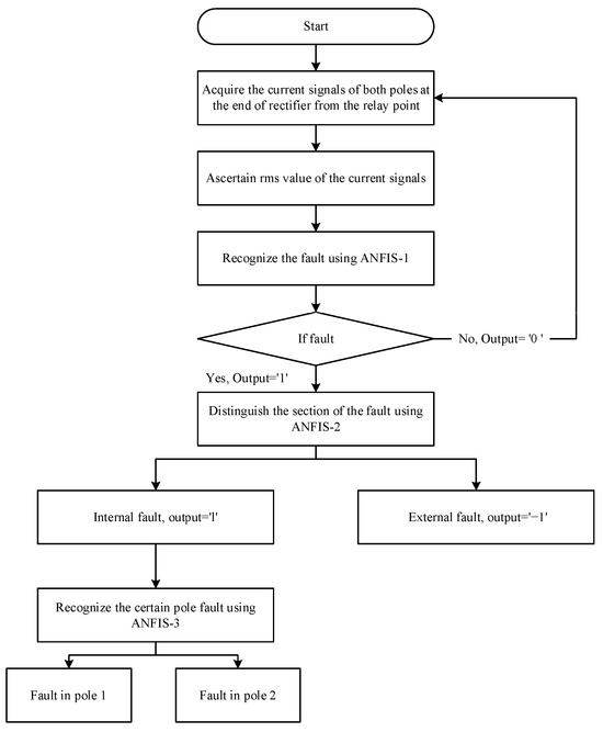
Figure 8.
The flowchart of the suggested method.
4.2. Application of Traditional Machine Learning in Cable Fault Localization
4.2.1. Artificial Neural Network
ANNs demonstrate strong performance in cable fault localization, with numerous researchers integrating them into diverse power system models. Farzad et al. [49] applied an ANN to an IEEE 34-bus test feeder incorporating two constant-speed wind turbines, proposing a fault location method for unbalanced distribution networks with DG integration. Figure 9 reveals that the global input yielded lower estimation errors than the local input. When the DG injection power is low, the ANN achieves low test errors even with local input alone. Furthermore, retraining the ANN with input data containing measurement errors maintained test errors within acceptable limits. In the following year, Farias et al. [50] introduced a novel HIF localization approach combining time-domain current-voltage equation solving with an online-trained ANN. This method utilizes fourth-order polynomial modeling and online ANN parameter estimation, eliminating reliance on additional measurement equipment or threshold adjustments. It achieves 2.3% maximum error for a 60 A base current fault located 10 km from the substation.
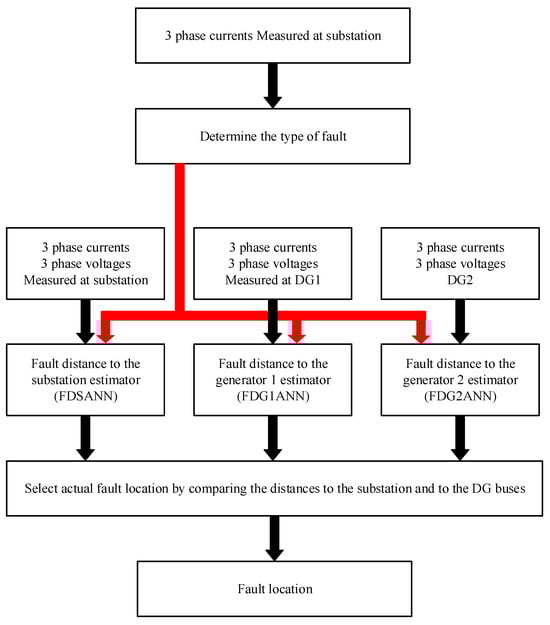
Figure 9.
Flowchart of the proposed fault location method.
In recent years, Hamidi et al. [51] utilized a multilayer perceptron (MLP) model to analyze the attenuation of traveling wave frequency components, incorporating principal component analysis (PCA) for feature dimensionality reduction. This approach offers advantages such as single-ended measurement, the elimination of communication infrastructure, and independence from time synchronization. To address the research gap in fault localization for AC microgrids, Jayasinghe et al. [52] employed an ANN for the rapid identification and localization of symmetrical and asymmetrical faults in AC microgrid distribution networks. The method achieves an MAE of 0.2122 in fault localization, demonstrating superior accuracy. Additionally, the proposed scheme generates outputs within a short response time, enabling rapid fault isolation to minimize potential damage to microgrids, which indicates promising prospects for real-time applications in AC microgrids.
4.2.2. Support Vector Machine
SVM has also been applied to cable fault localization. As early as 2014, Livani et al. [53] proposed a hybrid fault location method for transmission lines using an SVM classifier. The literature points out that inductance variations caused by aging degrade traveling wave velocity estimation, thereby deteriorating algorithm performance. To address this, a correction factor was introduced to convert cable parameter variations into velocity variations. Gashteroodkhani et al. [54] optimized SVM parameters with particle swarm optimization (PSO) to enhance classification accuracy, subsequently determining fault positions through Bewley lattice diagram analysis, as shown in Figure 10. The workflow is illustrated in the corresponding figure. The simulation results demonstrate that the proposed TT-SVM-PSO method achieves higher accuracy than the SVM-Wavelet approach in fault localization, while showing slightly slower computational speed. Recently, to tackle the difficulty in capturing wavefronts of traveling waves in submarine cables, Shuai et al. [55] developed a piecewise mapping model between time-domain features and fault distances using least squares SVM regression (LSSVR). This algorithm exhibits low data sample requirements, computational simplicity, and high precision, with robustness against varying fault resistances, measurement noise, and distributed cable parameters. Experimental validation on an RT-LAB-based hardware-in-the-loop platform confirms that the trained fault location model remains applicable to cable parameter variations in real systems.
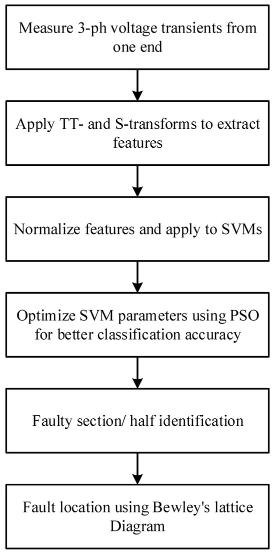
Figure 10.
Schematic diagram of the proposed method.
4.2.3. Genetic Algorithm
Genetic algorithms (GAs) are heuristic optimization algorithms that simulate the biological evolutionary process, efficiently searching for global optimal solutions within the solution space by mimicking mechanisms of natural selection, genetic mutation, and population mating. Their fundamental concept involves encoding problem solutions as chromosomes, constructing an initial population, evaluating individual fitness based on a fitness function, and iteratively refining the solution set through genetic operations such as selection, crossover, and mutation. Here, chromosomes are strings representing proposed solutions to the problem. Depending on the specific problem, a chromosome can be a string of discrete variables, binary values, or continuous values. The design of the chromosome and its parameters depends on the specific requirements of the problem being solved. This algorithm features characteristics like parallel search and strong robustness, making it particularly suitable for solving optimization problems involving complex nonlinear data in power systems.
Liang et al. [56] proposed a novel single-phase grounding fault localization method for distribution networks based on zero-sequence component distribution characteristics, transforming the fault location problem into optimizing the maximum value of the zero-sequence voltage drop (ZVD) function. The method solves this optimization using GA and achieves precise fault location. Simulation validations demonstrate its strong robustness under various fault conditions, with maximum location error below 0.22%. To address the bidirectional power flow caused by DG integration, Mohajer et al. [57] introduced a distribution time-domain line model-based fault localization method where fault distances and resistances were discretized and optimized via GA. The implementation workflow is detailed in Figure 11. The results show that localization accuracy remains minimally affected by fault distances, resistances, and inception angles, with improved precision observed alongside increasing DG penetration. In 2023, Psaras et al. [58] presented a fault localization technique for HVDC grids combining GA with reconstructed frequency-domain voltage profiles. For DC cable simulations, this method achieves maximum and average errors of 0.326% and 0.070%, respectively, across all fault scenarios, demonstrating excellent adaptability to long transmission lines and measurement noise while maintaining strong engineering applicability. Hardware-in-the-loop experiments on PSCAD/EMTDC confirm the trained model’s effectiveness against cable parameter variations in real systems.
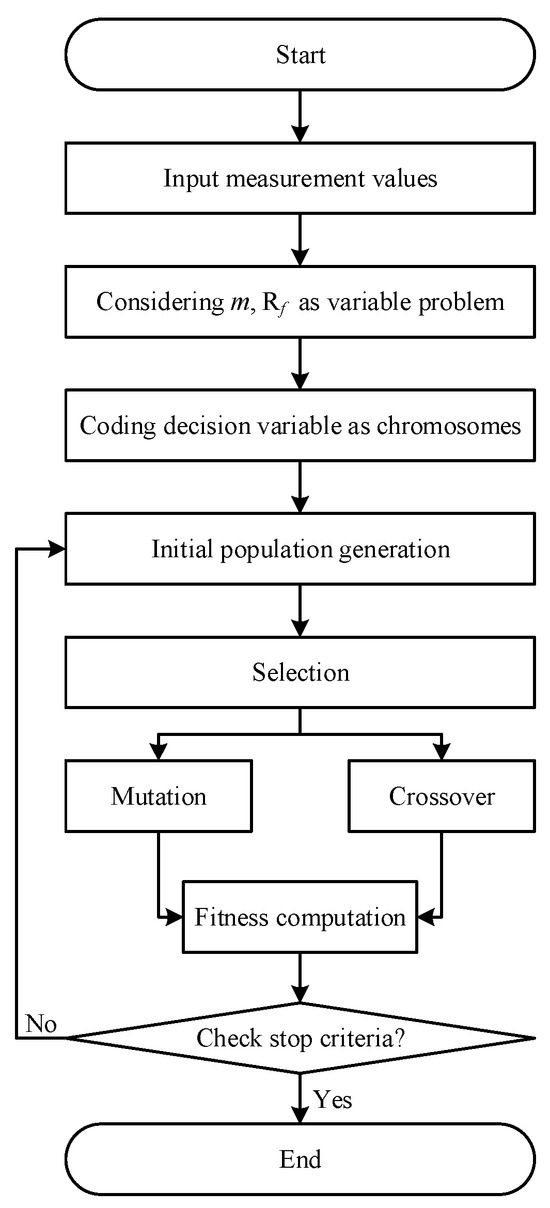
Figure 11.
Flowchart of GA for optimization problems.
5. Methods for Cable Fault Detection and Localization Based on Deep Learning
In recent years, the breakthroughs in computational capabilities have enabled deep learning (DL) to be applied in large-scale data domains such as image recognition and big data mining analysis. The continuous advancement of smart grids has driven the deployment of more intelligent devices and sensors within power systems, while the large-scale integration of DG exacerbates the uncertainty and nonlinearity of monitoring data. Therefore, DL demonstrates strong compatibility with cable fault detection, identification, and localization tasks, emerging as a powerful solution for addressing the complexities of modern smart grids.
5.1. Application of Deep Learning in Cable Fault Detection
5.1.1. Attention Mechanism
The attention mechanism originates from the selective focus of the human visual system on key information [59]. Its core principle is to enable the model to concentrate on task-relevant features by calculating the weight distribution among elements in the input sequence. Mathematically, its essence is a weighted summation process involving the Query and Key-Value. First, the input is mapped into three sets of vectors: Query, Key, and Value. Weights are then generated by calculating the similarity between the Query and the Key, and the output is obtained by performing a weighted aggregation of the Value. A schematic diagram of this process is shown in Figure 12. Typically, a set of queries computing the attention function is designated as matrix Q, while the Key and Value are designated as matrices K and V, respectively. The output matrix is then calculated as follows:
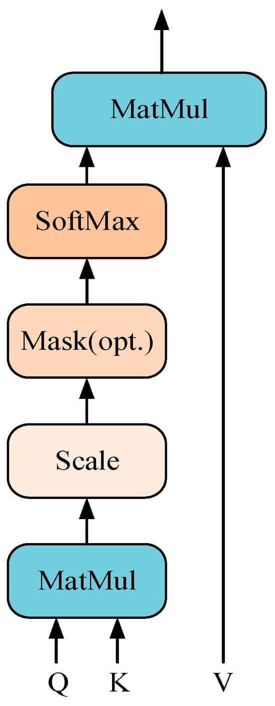
Figure 12.
Attention mechanism diagram.
In the equation, dk is the dimension of K. Scaling by stabilizes gradient updates during training.
Recently, researchers have begun applying attention mechanisms to cable fault detection. Peng et al. [60] developed an attention-based intelligent detection technique for grounding hazards in substation OPGW optical cables. Their approach integrates a convolutional block attention module (CBAM) into the backbone network of YOLOv5, incorporating both channel and spatial attention mechanisms, as illustrated in Figure 13. Simulation results reveal an error margin below 1%, demonstrating superior accuracy and stability in fault detection. It should be further noted that the more advanced YOLOv12 framework currently exists and has reached practical applicability. In future research, consideration could be given to replacing the existing network framework by introducing this more advanced YOLO framework, in order to explore its performance and application potential in relevant task scenarios.
Figure 13.
CBAM module.
Transformer is a deep neural network architecture based on a self-attention mechanism. Li et al. [61] proposed a PD pattern recognition method for power cables using Swin Transformer, introducing a cosine annealing learning rate scheduling mechanism to regulate the learning rate, termed Swin Transformer II. By partitioning windows and shifting computations to calculate local window attentions, Swin Transformer reduces computational complexity while capturing richer global information compared to conventional Vision Transformer. Experimental results demonstrate that the optimized Swin Transformer algorithm achieves higher accuracy in small-sample classification tasks, suitable for real-time PD diagnosis and enabling predictive maintenance in smart grids. Shu et al. [62] adopted an alternative framework called CSCRFAM-Transformer for fault identification in transmission lines through traveling wave measurements. The CSCRFAM module extracts features across channel and spatial dimensions, while the self-attention mechanism in Transformer reweights feature maps to enhance feature extraction precision, providing support for traveling wave acquisition devices in smart grid applications.
5.1.2. Convolutional Neural Network
Convolutional Neural Networks (CNNs) achieve hierarchical feature extraction through local connections, weight sharing, and pooling operations. Input data is first processed by convolutional layers, where different convolutional kernels compute inner products with local regions to extract low-level features such as edges and textures. Typically, for a single-channel input, the processing formula for a convolutional layer is as follows:
In the equation, k is the convolutional kernel size, i and j represent the output position, and b is the bias term. Pooling layers reduce parameter dimensionality through downsampling, enhancing feature translation invariance. After alternating multiple convolutional and pooling layers, a fully connected layer integrates the features and outputs classification or regression results. Specifically, the convolution operation leverages the properties of local receptive fields and weight sharing to capture spatial local patterns in the input data layer by layer, while nonlinear activation functions enhance representational capacity. Pooling layers compress feature dimensions to improve computational efficiency and translation invariance. During backpropagation, the error is propagated layer by layer through the network, updating the convolutional kernel weights and biases. In cable fault detection, CNNs can directly process time-frequency representations of signals, using convolutional kernels to capture high-frequency components of waveforms while suppressing noise through pooling operations.
Researchers have increasingly leveraged CNNs’ image recognition capabilities for cable fault detection, identification, and diagnosis. Wang et al. [63] integrated DWT, the Lorenz chaotic system, and a CNN to identify cable insulation faults, where DWT-denoised partial discharge signals are processed by the Lorenz system to generate dynamic error scatter plots, followed by CNN-based feature extraction for image prediction and classification. This model achieves 97.5% accuracy in identifying cable insulation fault types, significantly improving maintenance efficiency for power equipment. Li et al. [64] proposed an online insulation monitoring system for distribution network cables based on line conduction characteristics combined with a CNN algorithm. The system automatically learns and identifies insulation degradation trends and latent faults through data analysis, providing scientific decision-making support for power utilities.
Residual network (ResNet) is an innovative architecture addressing gradient vanishing and degradation issues in deep CNN training. Its core mechanism introduces shortcut connections within residual blocks, adding the output of convolutional layers to the original input, thereby enforcing residual mapping learning instead of direct target function approximation. Ding et al. [65] developed a tri-core cable fault line identification method combining ground current analysis with BiGRU-ResNet-MA, with the workflow illustrated in Figure 14. The BiGRU component extracts temporal features from ground current signals, while ResNet18 captures MTF image characteristics. A multi-head attention module reduces feature dimensionality and computational complexity by integrating multi-branch information to enhance model performance and robustness. Comparative experiments show that BiGRU-ResNet-MA achieves 100% training accuracy, outperforming GRU and CNN networks. In radial distribution network and IEEE-13 bus model testing, fault identification accuracy reaches 100% and 99.3%, respectively.
Figure 14.
Faulted identification model based on BiGRU-ResNet-MA.
5.1.3. Deep Belief Network
A Deep Belief Network (DBN) is a generative deep learning model formed by stacking multiple layers of Restricted Boltzmann Machines (RBMs), possessing capabilities for both unsupervised pre-training and supervised fine-tuning [66]. An RBM, in turn, is a generative stochastic artificial neural network that learns the probability distribution of its input dataset. As shown in the simplified RBM model in Figure 15, we assume the number of nodes in the visible layer is m and the number of nodes in the hidden layer is n. The energy function of a standard RBM is then defined as:
Figure 15.
Simplified model diagram of RBM.
In the equation, θ is the training dataset of the energy function, ω is the weight between the courseware node j and the hidden node i, and a and b are the offsets of the visible node j and the hidden node i, respectively. The core principle of DBN is to realize hierarchical abstraction of features through greedy layer-by-layer training of RBM: the bottom RBM takes the input data as the visible layer, models the probability dependency relationship between the visible layer and hidden layer through the energy function, and learns the initial feature representation of the data; the upper RBM then takes the output of the bottom hidden layer as input, iteratively extracts more abstract high-level features, and ultimately forms a mapping chain from raw data to abstract semantics. After pre-training is completed, supervised fine-tuning is performed on the entire network through backpropagation to optimize classification or regression objectives.
Qin et al. [67] established an underground distribution system containing 16 cable groups and proposed a DBN-based fault recognition model, achieving identification accuracy between 90 and 99% for grounding, short-circuit, and open-circuit faults, with open-circuit faults showing the highest recognition rate. As shown in Table 4, compared to traditional shallow networks such as BP neural network, annealed chaotic competitive learning network (ACCLN), and SVM, DBN attains an average fault identification accuracy of 97.8%, surpassing conventional methods and demonstrating its effectiveness in handling large-scale cable fault data. In 2023, Wan et al. [68] exploited DBN’s strong generalization and feature extraction capabilities for efficient and accurate cable fault recognition. This approach utilizes cable head-end input impedance spectra and time-frequency domain impedance spectra as identification features, achieving 99.27% fault recognition accuracy. The experimental results validate its practical applicability in smart-grid scenarios.
Table 4.
Average correct cable fault recognition rate (%).
5.2. Application of Deep Learning in Cable Fault Localization
5.2.1. Convolutional Neural Network
Cable fault localization primarily employs a one-dimensional convolutional neural network (1D-CNN). This sequence-oriented deep learning model utilizes sliding one-dimensional convolution kernels along temporal sequences to extract local features, combined with pooling operations for dimensionality reduction and robustness enhancement, demonstrating efficiency and lightweight advantages in sequential modeling. Wu et al. [69] implemented a hybrid architecture integrating a sparse autoencoder (SAE) with CNN, with the workflow depicted in Figure 16. The system employs D-CNN for output aging probabilities for cable segments and L-CNN to determine aging start/end positions and severity levels, with maintenance or monitoring strategies subsequently formulated based on combined model outputs. Said et al. [70] proposed a 1D-CNN-binary SVM (BSVM) coupled framework for fault classification and localization in nuclear plant underground cables. Using three-phase current data for prediction, the model maintains a maximum processing time below 0.15 s and maximum localization error within 0.095% across varying fault types, resistances, and initiation angles, validating its high-precision localization performance and real-time applicability.
Figure 16.
Flowchart of the proposed aged segment detection and location framework.
To reduce measurement costs, Lan et al. [71] proposed a data-efficient high-voltage cable fault localization framework that employs a CNN to identify coaxial wave arrival times, selects the most frequently occurring result as the final wave arrival time, and calculates fault distance based on the time difference of coaxial mode wave propagation to both terminals. The experimental results demonstrate that this approach requires fewer sensors, achieves high localization accuracy under multiple fault conditions, and successfully resolves the conflict between localization precision and measurement costs. Tsotsopoulou et al. [72] exploited CNN’s image processing capabilities by extracting image features from spectrograms to estimate fault positions along superconducting cables (SCs). Comparative studies validate that the CNN-based scheme outperforms LSTM-based approaches in fault localization accuracy, highlighting its practical advantages for real-world cable monitoring applications.
5.2.2. Long Short-Term Memory Network
The Long Short-Term Memory network (LSTM) is an improved variant of the RNN [73]. It addresses the long-distance dependency and gradient vanishing problems inherent in traditional RNNs through a gating mechanism. Its working principle is specifically illustrated in Figure 17. Its core unit is the memory cell, where the forget gate, input gate, and output gate collaboratively control information flow: the forget gate determines which historical information in the cell state needs to be discarded, the input gate processes new information at the current timestep and updates the cell state, and the output gate determines the current output based on the cell state and the hidden layer output. The specific process is as follows: the input sequence is first filtered by the forget gate to remove irrelevant historical information; the input gate generates update quantities via the sigmoid and tanh functions; these are then element-wise multiplied with the original cell state to complete the state iteration; finally, the output gate combines the cell state and the hidden layer activation value to generate the output for the current timestep.
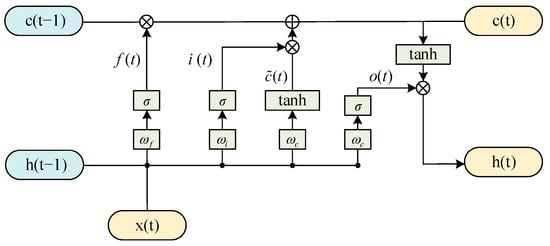
Figure 17.
Schematic diagram of LSTM working principle.
Current research leverages LSTM’s capability to manage short- and long-term memory in time-series data processing, often integrating it with other algorithms. Swaminathan et al. [74] proposed a CNN-LSTM deep learning framework for underground cable fault localization, taking two-dimensional data containing three-phase voltage and current signals as input, where LSTM layers and fully connected layers are employed to predict fault positions. Compared with other models, the CNN-LSTM-based approach better captures system nonlinearity and demonstrates superior performance. To resolve challenges of traditional time–frequency domain reflectometry (TFDR) in detecting cable joint faults, Chang et al. [75] introduced an unsupervised neural model combining LSTM and variational autoencoder (VAE). This model achieved fault localization errors of 1.774% and 1.015% for cable defects and joint defects, respectively, with experimental results validating the effectiveness of the proposed anomaly scoring method. Fu et al. [76] developed an LSTM-based approach integrated with resonance frequency analysis for fault detection and localization in underground power cables. After collecting fault current and resonance frequency data, the LSTM network processes the data to predict fault locations, with the specific algorithmic workflow illustrated in Figure 18. The results demonstrate that this method achieves high localization accuracy, with an average error of 0.6% and a maximum error of 1.8%, while exhibiting strong robustness across diverse fault scenarios.
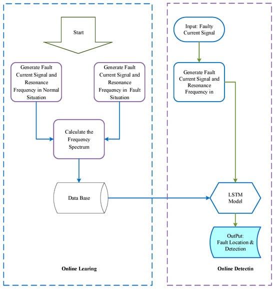
Figure 18.
Flowchart of the proposed algorithm.
5.2.3. Graph Convolutional Network
The Graph Convolutional Network (GCN) is a deep learning model for processing graph-structured data. Its core lies in jointly modeling the topological structure and node features to achieve information propagation. Its principle is based on the graph’s adjacency matrix A and node feature matrix X. By leveraging spectral decomposition of the Laplacian matrix or spatial domain neighborhood aggregation, it extends the convolution operation to non-Euclidean space. The propagation formula for a typical layer is:
In the equation, σ is the activation function, is the adjacency matrix with self-loops, is the corresponding degree matrix, and and are the node representation and trainable weight matrix of the lth layer, respectively. The normalization operation ensures stable feature aggregation for nodes with different degrees. Through multi-layer stacking, GCN enables each node to progressively aggregate feature information from k-hop neighbors, achieving an integrated representation of topological structure and node attributes. In power systems, GCN can map grid nodes to graph nodes and lines to edges. By combining node features with the network topology, it effectively captures the topological dependencies during cable faults.
Hu et al. [77] developed an MLP-GCN hybrid approach for fault localization in urban distribution networks by integrating MLP with GCN. This model demonstrates adaptability to network topology variations and exhibits fault tolerance for unknown data compared to conventional methods, while reducing dependency on fault current and voltage data through its enhanced practical performance. To address increased localization difficulty caused by massive distributed energy integration, Ma et al. [78] proposed a GCN-based fault localization framework for high-penetration DG distribution networks in 2024, which effectively captures spatial dependencies between nodes with strong robustness. As shown in Table 5, the simulation results validate that the model’s comprehensive performance surpasses both RF and CNN models across five metrics: accuracy, training time, F1-score, AUC value, and single inference time.
Table 5.
Fault location and electrical parameters.
6. Discussion
The above provides a detailed analysis of various methods for cable fault detection and localization. This section will summarize the advantages and disadvantages of these AI methods and elaborate on the challenges brought by DG access.
6.1. Advantages of AI Methods
Table 6 and Table 7 list and summarize all parameters of artificial intelligence technology in fault detection and localization methods. Comparative analysis of these studies reveals that next-generation AI technologies consistently demonstrate improved recognition accuracy, reduced localization error rates, and enhanced applicability to increasingly complex operational scenarios. This advancement stems from AI’s capability to perform real-time, rapid processing of large-scale data while conducting comprehensive analysis of multiple features, thereby exhibiting strong adaptability to diverse fault types.
Table 6.
Summary of fault detection methods based on AI (N/A: Information not available in the reference paper).
Table 7.
Summary of fault localization methods based on AI. (N/A: Information not available in the reference paper).
6.1.1. Nonlinear Feature Extraction
Cable fault signals typically manifest as traveling waves, zero-sequence currents/voltages, or partial discharge patterns, characterized by high dimensionality, nonstationarity, and significant noise interference. Traditional methods heavily rely on handcrafted features, making it challenging to capture complex signal patterns. AI introduces nonlinear transformations through activation functions, theoretically enabling the approximation of any continuous function complexity via the universal approximation theorem. Unlike conventional linear regression models constrained by superposition principles, MLP [51] constructs high-order feature interactions through cascading operations of hidden layer nodes, effectively decoupling nonlinear interdependencies between variables, while LSTM-based temporal models [74,75] decode dynamic evolution patterns of fault signals by modeling nonlinear temporal dependencies via gated mechanisms. These algorithms demonstrate powerful capabilities in processing nonlinear fault signals, thereby enhancing data analysis effectiveness and reliability.
6.1.2. Efficient Processing of Complex Data
With the rapid advancement of smart grid development, the volume of data generated by power grids has exhibited exponential growth. This explosive data expansion stems from both the inherent complexity of modern power systems and significant advancements in data acquisition technologies. The increasing scale and diversity of data impose higher demands on cable fault detection, identification, and localization. Artificial intelligence addresses these challenges through parallel computing capabilities. Specifically, AI leverages the tensor cores in graphics processing units and parallel computing architectures to accelerate matrix operations by orders of magnitude. Transformer-based models [61,62] enable parallel computation via multi-head attention mechanisms, while distributed training frameworks dramatically reduce the training time for deep residual networks on large-scale datasets [65]. Consequently, AI-driven methodologies can process massive grid data in real time, enabling rapid response and analysis for smart grids. This enhances operational agility in anomaly handling and ensures secure, stable system performance across dynamic operating environments.
However, significant differences exist in computational complexity and resource requirements among various AI technologies. These differences directly impact their practical applicability and computational efficiency when processing power grid data. Table 8 provides a comparative analysis of the computational complexity and resource demands for the five deep learning algorithms discussed in this paper. Consequently, given the multi-source nature of cable fault data and stringent real-time processing requirements, it is imperative to conduct a fine-grained analysis of an algorithm’s computational complexity and resource consumption based on the specific application scenario. This analysis is essential for constructing AI solutions that effectively balance accuracy and efficiency.
Table 8.
Summary of computational complexity and resource requirements for partial deep learning algorithms.
6.1.3. Adaptive Learning and Dynamic Optimization
With DG integration, associated fault signals exhibit uncertainty and intermittency, making fixed thresholds or empirical rules insufficient for adapting to grid dynamics. AI demonstrates technical superiority in adaptive learning and dynamic optimization, primarily through algorithmic architectures with real-time responsiveness to evolving environments and intelligent parameter space exploration mechanisms. GCN [77,78] enables non-Euclidean space modeling through graph structure encoding, while CNN [72] leverages translational invariance of regular grids by incorporating offset learning via deformable convolution for parameter optimization. This optimization breaks through the limitations of traditional approaches in cable fault feature extraction and correlation analysis, minimizing manual processing while enhancing decision-making efficiency and accuracy to better meet grid security requirements under complex operating conditions.
6.2. Limitations of AI Methods
While AI has enhanced the efficiency and automation of power systems in cable fault detection, identification, and localization, its development faces several limitations.
6.2.1. High Data Dependency
AI methods rely on data-driven training, yet practical scenarios suffer from the limited availability of fault samples and the severe class imbalance across fault types. Current solutions, such as augmenting data through noise addition, stretching, and translation, fail to fundamentally improve sample diversity. The accurate labeling of fault types and locations requires manual expertise or simulation tools, which are time-consuming and labor-intensive. Laboratory-generated simulation data often deviate from real-world conditions in noise levels and grounding resistance ranges, degrading model generalization. Consequently, the lack of high-quality fault signal data hinders progress in AI-based cable fault diagnosis.
To address this challenge, future research in related fields can systematically integrate the following strategies: at the data collection level, active exploration of multi-source data fusion pathways should be pursued, including (1) deepening collaboration with grid operators to establish long-term, standardized field fault signal acquisition mechanisms covering broader grounding resistance ranges and noise environments; (2) constructing high-standard, multi-condition cable fault physical simulation platforms [79] to generate synthetic data closely replicating real electromagnetic transient characteristics and noise spectra; and (3) promoting cross-regional, inter-institutional fault data sharing consortia under strict desensitization and compliance protocols to integrate fragmented small-sample resources. Moreover, advanced preprocessing and enhancement frameworks urgently require development, such as (1) implementing in-depth cleaning tailored to cable signal characteristics [80] for the accurate identification and repair of distorted segments and (2) applying joint time–frequency domain enhancement through random scaling and frequency band perturbation on S-transform or HHT spectra.
6.2.2. Poor Dynamic Environment Adaptability
AI models are typically trained on fixed topological structures, whereas cable operational topologies may dynamically shift over time or under environmental stress. For instance, humid conditions can degrade sensor signal fidelity, while equipment aging-induced shifts in cable traveling wave propagation characteristics may occur. Failure to update models in response to these variations risks performance degradation and erroneous judgments. Therefore, real-time model adaptation is essential during deployment to address evolving operational conditions, further enhancing grid operational stability and economic efficiency.
6.2.3. Limited Decision Trustworthiness
The ‘black-box’ nature of AI algorithms, particularly in deep learning models like CNNs, LSTMs, and DBNs, undermines interpretability. These models extract high-dimensional features through nonlinear transformations, obscuring decision logic and reducing operator trust in fault identification results. Trustworthiness challenges also manifest in precision validation. Traditional physics-based fault localization relies on quantifiable electromagnetic theory, while AI predictions depend on training data distributions. Deviations between training data and real-world conditions may cause localization errors exceeding engineering tolerances. Future research should prioritize hybrid frameworks integrating knowledge-driven and data-driven approaches to balance accuracy, efficiency, and transparency.
Current research in the field of cable fault identification and location is witnessing a progressive increase in studies concerning explainable AI (XAI) [81]. Explainability not only enhances users’ understanding and trust in AI models but also assists users in refining and optimizing these models upon identifying their shortcomings. To overcome these limitations, signal processing methods and physical mechanism modeling approaches represent two widely utilized methodologies [82]:
- Networks designed based on domain-specific signal processing knowledge require designers to possess expert experience; they utilize signal processing tools to extract signal patterns and prior knowledge from data, which are then translated into network architectures and optimization objectives. However, the acquisition of signal priors heavily relies on expert experience, and unreasonable signal priors can severely impair network performance; furthermore, some designs focus solely on network inputs and outputs, leaving the internal network structure unexplainable. Such studies remain relatively scarce and are primarily applied in fault diagnosis [83].
- Integrating physical models with deep network technology represents a highly promising developmental direction. Specifically, network architectures can be mapped to experimental data, and existing physical models can be fused with data-driven approaches. However, the design of network structures under this paradigm typically depends on the specific model structure, while different application scenarios demand tailored network architectures; moreover, it imposes stringent requirements on the physical model’s structure, making the use of complex physical models challenging. This paradigm has already been applied to solving fault identification [84] and fault location [85] problems.
6.3. Impact of DG Integration
After integrating DGs into the distribution grid, their operation may result in current reversal, transforming the network from a passive structure to an active one with diverse power source locations, thereby altering the original power flow distribution and fault current paths. Additionally, DGs can be reconfigured via Remote Control Switches (RCS), with flexible connection modes, locations, and operational strategies that significantly modify system topology. This leads to intermittent and temporal output signals, degrading their inherent features and properties and increasing challenges in fault detection and localization.
Among these DG models, those with stable outputs, such as diesel and gas turbine generators, have well-established reliability frameworks. In contrast, DGs like wind, solar, and energy storage systems exhibit notable volatility [86]. For instance, wind power generation correlates with wind speed, while photovoltaic output depends on solar irradiance and temperature, which vary considerably across different times of the day and display strong temporal characteristics. These factors collectively complicate DG output power modeling, creating inconsistencies in fault detection and localization approaches. Electric vehicle charging units, as typical nonlinear DGs, possess power electronic switching characteristics that induce current waveform distortion, leading to issues such as THD exceedance, three-phase imbalance, and voltage flicker [87]. Furthermore, the fluctuating outputs from PV and wind DGs combined with uncoordinated EV charging behaviors may exacerbate voltage fluctuations and frequency deviations in microgrids, impairing feature signal extraction. Currently, AI integration has provided effective solutions, with adaptive protection systems and advanced communication infrastructure supporting the dynamic behaviors of these DG units. Looking forward, more emphasis will be placed on integrating artificial intelligence into these fields to enhance fault detection and management capabilities.
7. Conclusions
This review introduces traditional machine learning and deep learning approaches in cable fault detection and localization, summarizing their respective advantages, disadvantages, and recent advancements. As distribution networks become increasingly complex and intelligent, integrating artificial intelligence algorithms into existing methods is critical to ensure broad adaptability across diverse power systems. Based on the analysis presented, current cable fault detection and localization techniques can be enhanced in three key areas:
- (1)
- Recent studies on fault line selection have achieved progress, particularly with adjustments to traditional methods in response to widespread DG integration. However, most existing research relies on simulated signal data derived from cable and power system models, neglecting the influence of actual cable installation conditions and environmental factors on current signals. This oversight leads to suboptimal performance in real-world applications. Future efforts should focus on developing fault feature computation models for active distribution networks, exploring topology identification strategies for DG-integrated grids, and incorporating cable structural impacts on fault currents to enhance the reliability of fault line selection.
- (2)
- Expanding the integration of advanced AI techniques. With the evolution of AI and deep learning, adopting next-generation AI for cable fault detection and localization has become inevitable. Sophisticated deep learning models leveraging convolutional or attention mechanisms can better handle nonlinear features and adaptively address complex grid operational states, enabling in-depth extraction and accurate identification of fault characteristics. Their self-learning and optimization capabilities also allow protective relaying systems to dynamically adapt to grid changes, improving robustness and flexibility. However, limited fault sample data and severe class imbalance in distribution networks often result in misjudgments when directly applying deep learning. To address this, generating synthetic datasets reflecting real-world conditions and enriching training data for AI-based line selection methods will be essential.
- (3)
- Current distribution networks typically rely on advanced measurement systems such as fault recorders, traveling wave detectors, and phasor measurement units to capture high-quality steady-state or transient electrical signals. These systems enable high precision and speed in identifying grounding or interphase faults. However, the vast and branched structure of China’s distribution grid, combined with DG integration, creates highly variable operational scenarios. Deploying such measurement systems incurs significant costs, posing challenges for practical engineering applications. Future research should prioritize optimizing measurement device placement based on grid topology to minimize installation numbers while balancing economic efficiency and computational effectiveness.
Author Contributions
Validation, S.F. and Z.Z.; investigation, Q.S., Z.F., S.F. and Z.M.; data curation, S.F., Z.Z. and F.L.; writing—original draft preparation, Q.S., F.L. and Z.M.; writing—review and editing, Q.S., Z.F. and P.L.; visualization, S.F., Z.Z. and P.L.; supervision, Q.S. and P.L.; project administration, F.L. and Z.M.; funding acquisition, Z.F. All authors have read and agreed to the published version of the manuscript.
Funding
This research was funded by the Key Scientific and Technical Funds of Sichuan Electric Power Corporation, The Rapid Isolation and Transfer Technology for Single-Phase Ground Faults in Cable Lines, grant number 52199723002N.
Conflicts of Interest
The authors declare no conflict of interest.
Abbreviations
The following abbreviations are used in this manuscript:
| AI | Artificial intelligence |
| IoT | Internet of Things |
| XLPE | Cross-linked polyethylene |
| HVDC-VSC | High-voltage direct current voltage source converter |
| PD | Partial discharge |
| PV | Photovoltaic |
| GWC | Grounding wire current |
| FIA | Fault inception angles |
| DWT | Discrete wavelet transform |
| CWT | Continuous wavelet transform |
| EWT | Empirical wavelet transform |
| MRSVD | Multi-resolution singular value decomposition |
| HFCT | High-frequency current transformers |
| FFT | Fast Fourier transform |
| NLT | Numerical Laplace transform |
| ANN | Artificial neural network |
| NNRBF | Neural Network with Radial Basis Function |
| PLC | Power Line Communication |
| SNR | Signal-to-noise ratio |
| SVM | Support Vector Machine |
| MCSVM | Multi-class support vector machine |
| OVO | One-versus-one |
| MV | Medium-voltage |
| ANFIS | Adaptive Neuro-Fuzzy Inference System |
| SD | Standard deviation |
| FLS | Fuzzy Logic Systems |
| MAE | Mean absolute error |
| RMSE | Root mean square error |
| HVDC | High-voltage direct current |
| MLP | Multilayer perceptron |
| PSO | Particle swarm optimization |
| LSSVR | Least squares SVM regression |
| GA | Genetic algorithm |
| ZVD | Zero-sequence voltage drop |
| DL | Deep learning |
| CBAM | Convolutional block attention module |
| CNN | Convolutional neural network |
| ResNet | Residual network |
| DBN | Deep belief network |
| ACCLN | Annealed chaotic competitive learning network |
| SAE | Sparse autoencoder |
| SC | Superconducting cable |
| LSTM | Long Short-Term Memory |
| TFDR | Time-frequency domain reflectometry |
| VAE | Variational autoencoder |
| GCN | Graph Convolutional Network |
References
- Dondi, P.; Bayoumi, D.; Haederli, C.; Julian, D.; Suter, M. Network integration of distributed power generation. J. Power Sources 2002, 106, 1–9. [Google Scholar] [CrossRef]
- Dehghanian, P.; Aslan, S.; Dehghanian, P. Maintaining Electric System Safety Through An Enhanced Network Resilience. IEEE Trans. Ind. Appl. 2018, 54, 4927–4937. [Google Scholar] [CrossRef]
- Choi, M.S.; Lee, S.J.; Lim, S.I.; Lee, D.S.; Yang, X. A Direct Three-Phase Circuit Analysis-Based Fault Location for Line-to-Line Fault. IEEE Trans. Power Deliv. 2007, 22, 2541–2547. [Google Scholar] [CrossRef]
- Mohammed, A.; Kora, R. A comprehensive review on ensemble deep learning: Opportunities and challenges. J. King Saud Univ.-Comput. Inf. Sci. 2023, 35, 757–774. [Google Scholar] [CrossRef]
- Archana, R.; Jeevaraj, P.S.E. Deep learning models for digital image processing: A review. Artif. Intell. Rev. 2024, 57, 11. [Google Scholar] [CrossRef]
- Zhang, Y.F.; He, Z.T.; Li, J.X.; Lin, J.F.; Guan, Q.F.; Yu, W.H. MapGPT: An autonomous framework for mapping by integrating large language model and cartographic tools. Cartogr. Geogr. Inf. Sci. 2024, 51, 717–743. [Google Scholar] [CrossRef]
- Metzger, S.L.; Littlejohn, K.T.; Silva, A.B.; Moses, D.A.; Seaton, M.P.; Wang, R.; Dougherty, M.E.; Liu, J.R.; Wu, P.; Berger, M.A.; et al. A high-performance neuroprosthesis for speech decoding and avatar control. Nature 2023, 620, 1037–1046. [Google Scholar] [CrossRef]
- IEC 60502-1:2004; Power Cables with Extruded Insulation and Their Accessories for Rated Voltages from 1 kV (Um = 1.2 kV) up to 30 kV (Um = 36 kV)—Part 1: Cables for Rated Voltages from 1 kV (Um = 1.2 kV) up to 6 kV (Um = 7.2 kV). International Electrotechnical Commission: Geneva, Switzerland, 2004.
- Li, G.; Wang, Z.; Lan, R.; Wei, Y.; Nie, Y.; Li, S.; Lei, Q. The Lifetime Prediction and Insulation Failure Mechanism of XLPE for High-Voltage Cable. IEEE Trans. Dielectr. Electr. Insul. 2023, 30, 761–768. [Google Scholar] [CrossRef]
- Li, Y.M.; Peng, Z.W.; Xu, D.G.; Huang, S.Y.; Gao, Y.F.; Li, Y. Research on the Thermal Aging Characteristics of Crosslinked Polyethylene Cables Based on Polarization and Depolarization Current Measurement. Energies 2024, 17, 2274. [Google Scholar] [CrossRef]
- Li, H.C.; Cai, J.; Chen, P.; Zhang, J.C.; Guo, W.; Pan, Z.H.; Qian, M.D. Effect of moisture on the electric field and breakdown voltage of XLPE cable interconnectors. AIP Adv. 2024, 14, 115221. [Google Scholar] [CrossRef]
- Afia, R.S.A.; Ehtasham, M.; Tamus, Z.Á. Electrical and Mechanical Condition Assessment of Low Voltage Unshielded Nuclear Power Cables Under Simultaneous Thermal and Mechanical Stresses: Application of Non-Destructive Test Techniques. IEEE Access 2021, 9, 4531–4541. [Google Scholar] [CrossRef]
- Afia, R.S.A.; Mustafa, E.; Tamus, Z.A. Comparison of Mechanical and Low-Frequency Dielectric Properties of Thermally and Thermo-Mechanically Aged Low Voltage CSPE/XLPE Nuclear Power Plant Cables. Electronics 2021, 10, 2728. [Google Scholar] [CrossRef]
- Karasin Pathirannahalage, A.N.P. Travelling Wave Based DC Line Fault Location in VSC HVDC Systems; University of Manitoba: Winnipeg, MB, Canada, 2013. [Google Scholar]
- Hassan, H.A.A.; Grainger, B.M.; McDermott, T.E.; Reed, G.F. Fault location identification of a hybrid HVDC-VSC system containing cable and overhead line segments using transient data. In Proceedings of the 2016 IEEE/PES Transmission and Distribution Conference and Exposition (T&D), Dallas, TX, USA, 3–5 May 2016; pp. 1–5. [Google Scholar]
- Verrax, P.; Alglave, N.; Bertinato, A.; Kieffer, M.; Raison, B. Low-complexity graph-based traveling wave models for HVDC grids with hybrid transmission lines: Application to fault identification. Electr. Power Syst. Res. 2022, 205, 107710. [Google Scholar] [CrossRef]
- Shi, S.; Hu, Z.; Ma, Z.; Dong, X. Travelling waves-based identification of sub-health condition of feeders in power distribution system. IET Gener. Transm. Distrib. 2018, 12, 1067–1073. [Google Scholar] [CrossRef]
- Yan, Y.; Zhao, Y.; Zhao, K.; Trinchero, R.; Stievano, I.S.; Li, H. A high-efficiency portable system for insulation condition assessment of wind farm inter-array cables with double-sided partial discharge detection and localisation. IET Gener. Transm. Distrib. 2023, 17, 2523–2534. [Google Scholar] [CrossRef]
- Rajpoot, S.C.; Pandey, C.; Rajpoot, P.S.; Singhai, S.K.; Sethy, P.K. A Dynamic-SUGPDS Model for Faults Detection and Isolation of Underground Power Cable Based on Detection and Isolation Algorithm and Smart Sensors. J. Electr. Eng. Technol. 2021, 16, 1799–1819. [Google Scholar] [CrossRef]
- Peng, N.; Liu, X.; Liang, R.; Tang, Z.; Ren, X.; Hu, Y.; Li, G. Edge Computing Based Fault Sensing of the Distribution Cables Based on Time-Domain Analysis of Grounding Line Current Signals. IEEE Trans. Power Deliv. 2022, 37, 4404–4417. [Google Scholar] [CrossRef]
- Dashti, R.; Sadeh, J. Fault section estimation in power distribution network using impedance-based fault distance calculation and frequency spectrum analysis. IET Gener. Transm. Distrib. 2014, 8, 1406–1417. [Google Scholar] [CrossRef]
- Daisy, M.; Dashti, R. Single phase fault location in electrical distribution feeder using hybrid method. Energy 2016, 103, 356–368. [Google Scholar] [CrossRef]
- Adewole, A.C.; Tzoneva, R.; Behardien, S. Distribution network fault section identification and fault location using wavelet entropy and neural networks. Appl. Soft Comput. 2016, 46, 296–306. [Google Scholar] [CrossRef]
- Samet, H.; Khaleghian, S.; Tajdinian, M.; Ghanbari, T.; Terzija, V. A similarity-based framework for incipient fault detection in underground power cables. Int. J. Electr. Power Energy Syst. 2021, 133, 107309. [Google Scholar] [CrossRef]
- Zhang, P.; Jin, M.; Liang, R.; Tang, Z.; Hou, M.; Peng, N.; Li, J. Faulty Cable Segment Identification of Low-Resistance Grounded Active Distributions via Grounding Wire Current-Based Approach. IEEE Trans. Ind. Inform. 2024, 20, 7708–7718. [Google Scholar] [CrossRef]
- Zhang, P.; Hou, M.; Liang, R.; Tang, Z.; Li, J.; Jin, M.; Sun, Z.; Peng, N. Incipient Fault Detection of Medium-Voltage Distribution Cable Systems Using Time-Frequency Analysis of Grounding Wire Currents. IEEE Trans. Smart Grid 2025, 16, 74–86. [Google Scholar] [CrossRef]
- Deng, F.; Zeng, X.; Tang, X.; Li, Z.; Zu, Y.; Mei, L. Travelling-wave-based fault location algorithm for hybrid transmission lines using three-dimensional absolute grey incidence degree. Int. J. Electr. Power Energy Syst. 2020, 114, 105306. [Google Scholar] [CrossRef]
- Rezaei, D.; Gholipour, M.; Parvaresh, F. A single-ended traveling-wave-based fault location for a hybrid transmission line using detected arrival times and TW′s polarity. Electr. Power Syst. Res. 2022, 210, 108058. [Google Scholar] [CrossRef]
- Tariq, R.; Alhamrouni, I.; Rehman, A.U.; Tag Eldin, E.; Shafiq, M.; Ghamry, N.A.; Hamam, H. An Optimized Solution for Fault Detection and Location in Underground Cables Based on Traveling Waves. Energies 2022, 15, 6468. [Google Scholar] [CrossRef]
- Xie, L.W.; Luo, L.F.; Ma, J.J.; Li, Y.; Zhang, M.M.; Zeng, X.J.; Cao, Y.J. A novel fault location method for hybrid lines based on traveling wave. Int. J. Electr. Power Energy Syst. 2022, 141, 108102. [Google Scholar] [CrossRef]
- Huang, Z.; Fang, C.; Jiang, Q.; Hu, T.; Lv, J. Research on Tree Flash Fault Localization of Hybrid Overhead–Underground Lines Based on Improved Double-Ended Traveling Wave Method. Appl. Sci. 2024, 14, 4739. [Google Scholar] [CrossRef]
- Hasanvand, H.; Parastar, A.; Arshadi, B.; Zamani, M.R.; Bordbar, A.S. A comparison between S-transform and CWT for fault location in combined overhead line and cable distribution networks. In Proceedings of the 2016 21st Conference on Electrical Power Distribution Networks Conference (EPDC), Karaj, Iran, 26–27 April 2016; pp. 70–74. [Google Scholar]
- Haohao, C.; Jing, L.; Ping, C. Design of fault location algorithm based on online distributed travelling wave for HV power cable. PLoS ONE 2024, 19, e0296513. [Google Scholar] [CrossRef]
- Cifuentes, N.; Pal, B.C. A New Approach to the Fault Location Problem: Using the Fault’s Transient Intermediate Frequency Response. IEEE Open Access J. Power Energy 2021, 8, 510–521. [Google Scholar] [CrossRef]
- Song, G.; Yan, J.; Chang, Z.; Zhang, C.; Gao, X. A Frequency-Domain Fault Location Method for Underground Cables in MMC-HVdc Systems. IEEE Trans. Instrum. Meas. 2024, 73, 1–12. [Google Scholar] [CrossRef]
- Bretas, A.S.; Herrera-Orozco, A.R.; Orozco-Henao, C.A.; Iurinic, L.U.; Mora-Flórez, J. Incipient fault location method for distribution networks with underground shielded cables: A system identification approach. Int. Trans. Electr. Energy Syst. 2017, 27, e2465. [Google Scholar] [CrossRef]
- Ledesma, J.J.G.; do Nascimento, K.B.; de Araujo, L.R.; Penido, D.R.R. A two-level ANN-based method using synchronized measurements to locate high-impedance fault in distribution systems. Electr. Power Syst. Res. 2020, 188, 106576. [Google Scholar] [CrossRef]
- Gogula, V.; Edward, B. Fault detection in a distribution network using a combination of a discrete wavelet transform and a neural Network’s radial basis function algorithm to detect high-impedance faults. Front. Energy Res. 2023, 11, 1101049. [Google Scholar] [CrossRef]
- Bindi, M.; Luchetta, A.; Lozito, G.M.; Carobbi, C.F.M.; Grasso, F.; Piccirilli, M.C. Frequency Characterization of Medium Voltage Cables for Fault Prevention Through Multi-Valued Neural Networks and Power Line Communication Technologies. IEEE Trans. Power Deliv. 2023, 38, 3227–3237. [Google Scholar] [CrossRef]
- Hearst, M.A.; Dumais, S.T.; Osuna, E.; Platt, J.; Scholkopf, B. Support vector machines. IEEE Intell. Syst. Their Appl. 1998, 13, 18–28. [Google Scholar] [CrossRef]
- Abu-Rub, O.H.; Khan, Q.; Refaat, S.S.; Nounou, H. Cable Insulation Fault Identification Using Partial Discharge Patterns Analysis. IEEE Can. J. Electr. Comput. Eng. 2022, 45, 31–41. [Google Scholar] [CrossRef]
- Saad, M.H.; Said, A. Machine learning-based fault diagnosis for research nuclear reactor medium voltage power cables in fraction Fourier domain. Electr. Eng. 2023, 105, 25–42. [Google Scholar] [CrossRef]
- Razmi, P.; Pashaei, M.; Karimi, M.; Kauhaniemi, K.; Simoes, M.G. Data-Driven Intermittent Earth Fault Detection in Compensated and Isolated MV Networks. In Proceedings of the 2024 International Workshop on Artificial Intelligence and Machine Learning for Energy Transformation (AIE), Vaasa, Finland, 20–22 May 2024; pp. 1–6. [Google Scholar]
- Laib, A.; Melit, M.; Nekhoul, B.; Boudjefdjouf, H.; Bouchekara, H. Localisation of faults in wiring networks using time domain reflectometry and adaptive neuro-fuzzy inference system. Electron. Lett. 2017, 53, 600–601. [Google Scholar] [CrossRef]
- Veerasamy, V.; Abdul Wahab, N.I.; Ramachandran, R.; Mansoor, M.; Thirumeni, M.; Lutfi Othman, M. High Impedance Fault Detection in Medium Voltage Distribution Network Using Discrete Wavelet Transform and Adaptive Neuro-Fuzzy Inference System. Energies 2018, 11, 3330. [Google Scholar] [CrossRef]
- Veerasamy, V.; Abdul Wahab, N.I.; Ramachandran, R.; Thirumeni, M.; Subramanian, C.; Othman, M.L.; Hizam, H. High-impedance fault detection in medium-voltage distribution network using computational intelligence-based classifiers. Neural Comput. Appl. 2019, 31, 9127–9143. [Google Scholar] [CrossRef]
- Peddakapu, K.; Srinivasarao, P.; Mohamed, M.R.; Liu, X.N.; Kishore, D.J.K. Faults identification in high voltage direct current transmission lines using adaptive neuro-fuzzy inference system. Int. J. Model. Simul. 2023, 43, 813–831. [Google Scholar] [CrossRef]
- Kumari, R.; Naick, B.K. Enhancing protection in AC microgrids: An adaptive approach with ANN and ANFIS models. Comput. Electr. Eng. 2024, 115, 109103. [Google Scholar] [CrossRef]
- Dehghani, F.; Khodnia, F.; Dehghan, E. Fault location of unbalanced power distribution feeder with distributed generation using neural networks. CIRED 2017, 2017, 1134–1137. [Google Scholar] [CrossRef]
- Farias, P.E.; de Morais, A.P.; Rossini, J.P.; Cardoso, G. Non-linear high impedance fault distance estimation in power distribution systems: A continually online-trained neural network approach. Electr. Power Syst. Res. 2018, 157, 20–28. [Google Scholar] [CrossRef]
- Hamidi, S.M.; Ameli, A.; Ghafouri, M.; Lopes, F.V. A Learning-Based Framework for Locating Faults on Power Grid Lines Based on Distortion of Traveling Waves. IEEE Trans. Instrum. Meas. 2022, 71, 1–15. [Google Scholar] [CrossRef]
- Jayasinghe, J.A.R.R.; Malindi, J.H.E.; Rajapaksha, R.M.A.M.; Logeeshan, V.; Wanigasekara, C. Classification and Localization of Faults in AC Microgrids Through Discrete Wavelet Transform and Artificial Neural Networks. IEEE Open Access J. Power Energy 2024, 11, 303–313. [Google Scholar] [CrossRef]
- Livani, H.; Evrenosoglu, C.Y. A Machine Learning and Wavelet-Based Fault Location Method for Hybrid Transmission Lines. IEEE Trans. Smart Grid 2014, 5, 51–59. [Google Scholar] [CrossRef]
- Gashteroodkhani, O.A.; Majidi, M.; Etezadi-Amoli, M.; Nematollahi, A.F.; Vahidi, B. A hybrid SVM-TT transform-based method for fault location in hybrid transmission lines with underground cables. Electr. Power Syst. Res. 2019, 170, 205–214. [Google Scholar] [CrossRef]
- Shuai, Z.; Wu, L.; He, L.; Wan, J.; Wang, W.; Li, Y.; Zhou, Q.; He, Z.; Xu, Q. Fault Location Method Using Local Incipient Current Features for Submarine DC Power Systems. IEEE Trans. Instrum. Meas. 2025, 74, 1–15. [Google Scholar] [CrossRef]
- Rui, L.; Nan, P.; Zhi, Y.; Zare, F. A novel single-phase-to-earth fault location method for distribution network based on zero-sequence components distribution characteristics. Int. J. Electr. Power Energy Syst. 2018, 102, 11–22. [Google Scholar] [CrossRef]
- Mohajer, F.; Sadeh, J. Accurate fault location method for distribution network in presence of DG using distributed time-domain line model. IET Gener. Transm. Distrib. 2022, 16, 1305–1318. [Google Scholar] [CrossRef]
- Psaras, V.; Tzelepis, D.; Burt, G. HVDC grid fault location method using genetic algorithm on reconstructed frequency-domain voltage profiles. Int. J. Electr. Power Energy Syst. 2023, 144, 108429. [Google Scholar] [CrossRef]
- Tian, H.Y.; Wang, J.X.; Zhang, W.K.; Liu, H.; Song, Y.X.; Chen, W.G. 110 kV Power Cable External Disturbance Optical Fiber Sensing Detection and Identification Method Based on ResNeXt and Attention Mechanism. IEEE Trans. Instrum. Meas. 2025, 74, 1–11. [Google Scholar] [CrossRef]
- Peng, L.; Wang, S.; Yuan, J.; Pan, L.; Wang, M. Intelligent detection technology of potential grounding trouble of OPGW cable in substation based on attention model. Opt. Fiber Technol. 2025, 93, 104151. [Google Scholar] [CrossRef]
- Li, Y.; Gong, C.; Deng, T.; Jia, Z.; Wang, F.; Zhao, Q.; Zhang, J. Partial Discharge Pattern Recognition Based on Swin Transformer for Power Cable Fault Diagnosis in Modern Distribution Systems. Processes 2025, 13, 852. [Google Scholar] [CrossRef]
- Shu, H.; Liu, H.; Tang, Y.; Su, X.; Han, Y.; Dai, Y. Fault Identification Method for Measured Travelling Wave of Transmission Line Based on CSCRFAM-Transformer. Prot. Control Mod. Power Syst. 2025, 10, 69–82. [Google Scholar] [CrossRef]
- Wang, M.H.; Lu, S.D.; Liao, R.M. Fault Diagnosis for Power Cables Based on Convolutional Neural Network With Chaotic System and Discrete Wavelet Transform. IEEE Trans. Power Deliv. 2022, 37, 582–590. [Google Scholar] [CrossRef]
- Li, H.; Shao, H.; Niu, S. Online Monitoring Technology for Cable Insulation in Distribution Networks Based on Line Conduction Characteristics. Int. J. Inf. Technol. Syst. Approach 2024, 17, 1–17. [Google Scholar] [CrossRef]
- Ding, C.; Wang, F.; Li, S.; Jiang, C.; Ma, P. Three-Core Cable Fault Line Identification Based on Ground Wire Current and BiGRU-ResNet-MA. IEEE Access 2024, 12, 136120–136130. [Google Scholar] [CrossRef]
- Chen, Y.S.; Zhao, X.; Jia, X.P. Spectral-Spatial Classification of Hyperspectral Data Based on Deep Belief Network. IEEE J. Sel. Top. Appl. Earth Obs. Remote Sens. 2015, 8, 2381–2392. [Google Scholar] [CrossRef]
- Qin, X.; Zhang, Y.; Mei, W.; Dong, G.; Gao, J.; Wang, P.; Deng, J.; Pan, H. A cable fault recognition method based on a deep belief network. Comput. Electr. Eng. 2018, 71, 452–464. [Google Scholar] [CrossRef]
- Wan, Q.; Li, Y.; Yuan, R.; Meng, Q.; Li, X. Fault Identification and Localization of a Time−Frequency Domain Joint Impedance Spectrum of Cables Based on Deep Belief Networks. Sensors 2023, 23, 684. [Google Scholar] [CrossRef]
- Wu, Y.; Zhang, P.; Lu, G. Detection and Location of Aged Cable Segment in Underground Power Distribution System Using Deep Learning Approach. IEEE Trans. Ind. Inform. 2021, 17, 7379–7389. [Google Scholar] [CrossRef]
- Said, A.; Hashima, S.; Fouda, M.M.; Saad, M.H. Deep Learning-Based Fault Classification and Location for Underground Power Cable of Nuclear Facilities. IEEE Access 2022, 10, 70126–70142. [Google Scholar] [CrossRef]
- Lan, T.; Mazhari, S.M.; Teimourzadeh, H.; Chung, C.Y. An Online Data-Efficient HV Cable Fault Localization Approach Via an AI-Enabled Recognition of Modal Wavefront in Sheath Current. IEEE Trans. Power Deliv. 2023, 38, 1977–1989. [Google Scholar] [CrossRef]
- Tsotsopoulou, E.; Karagiannis, X.; Papadopoulos, T.; Chrysochos, A.; Dyśko, A.; Hong, Q.; Tzelepis, D. Advanced fault location scheme for superconducting cables based on deep learning algorithms. Int. J. Electr. Power Energy Syst. 2023, 147, 108860. [Google Scholar] [CrossRef]
- Cheng, J.; Dong, L.; Lapata, M. Long short-term memory-networks for machine reading. arXiv 2016, arXiv:1601.06733. [Google Scholar]
- Swaminathan, R.; Mishra, S.; Routray, A.; Swain, S.C. A CNN-LSTM-based fault classifier and locator for underground cables. Neural Comput. Appl. 2021, 33, 15293–15304. [Google Scholar] [CrossRef]
- Chang, S.J.; Kwon, G.Y. Anomaly Detection for Shielded Cable Including Cable Joint Using a Deep Learning Approach. IEEE Trans. Instrum. Meas. 2023, 72, 1–10. [Google Scholar] [CrossRef]
- Fu, H.; Qiu, L.; Ai, Y.; Tu, J.; Yan, Y. Deep learning-based fault detection and location in underground power cables using resonance frequency analysis. Electr. Eng. 2025, 107, 4051–4062. [Google Scholar] [CrossRef]
- Hu, Y.; Chen, J.; Ye, H.; Liu, Y.; Zhang, J.; Li, Y. Fault Location Method of Complex Urban Distribution Network Based on MLP-GCN. In Proceedings of the 2022 IEEE/IAS Industrial and Commercial Power System Asia (I&CPS Asia), Shanghai, China, 8–11 July 2022; pp. 1580–1585. [Google Scholar]
- Ma, X.P.; Zhen, W.X.; Ren, H.D.; Zhang, G.R.; Zhang, K.; Dong, H.Y. A Method for Fault Localization in Distribution Networks with High Proportions of Distributed Generation Based on Graph Convolutional Networks. Energies 2024, 17, 5758. [Google Scholar] [CrossRef]
- Sheng, W.X.; Liu, K.Y.; Liang, Y. Comprehensive fault simulation method in active distribution network with the consideration of cyber security. IET Cyber-Phys. Syst. Theory Appl. 2021, 6, 27–40. [Google Scholar] [CrossRef]
- Zhang, W.Z.; Cheng, D.B.; Lu, G.Q.; Zhou, B.; Li, J.Y.; Zhang, S.C. Efficient Adaptive Label Refinement for label noise learning. Neurocomputing 2025, 639, 130305. [Google Scholar] [CrossRef]
- Xu, C.; Liao, Z.; Li, C.; Zhou, X.; Xie, R. Review on Interpretable Machine Learning in Smart Grid. Energies 2022, 15, 4427. [Google Scholar] [CrossRef]
- Yan, R.; Shang, Z.; Wang, Z.; Xu, W.; Zhao, Z.; Wang, S.; Chen, X. Challenges and Opportunities of XAI in Industrial Intelligent Diagnosis: Priori-empowered. J. Mech. Eng. 2024, 60, 1–20. [Google Scholar]
- Kim, S.G.; Ryu, S.; Kim, H.; Jin, K.; Cho, J. Enhancing the Explainability of AI Models in Nuclear Power Plants with Layer-wise Relevance Propagation. In Proceedings of the Transactions of the Korean Nuclear Society Virtual Autumn Meeting, Jeju, Republic of Korea, 21–22 October 2021. [Google Scholar]
- Wali, S.; Khan, I. Explainable Signature-based Machine Learning Approach for Identification of Faults in Grid-Connected Photovoltaic Systems. In Proceedings of the 2022 IEEE Texas Power and Energy Conference (TPEC), College Station, TX, USA, 28 February–1 March 2022; pp. 1–6. [Google Scholar]
- Liu, Y.; Zhang, N.; Wu, D.; Botterud, A.; Yao, R.; Kang, C. Searching for Critical Power System Cascading Failures With Graph Convolutional Network. IEEE Trans. Control Netw. Syst. 2021, 8, 1304–1313. [Google Scholar] [CrossRef]
- Peddakapu, K.; Mohamed, M.R.; Harika, R.P.; Srinivasrao, P.; Licari, J. Climate-adaptive battery solutions for renewable microgrids: A case study in Indian coastal and inland regions. Energy 2024, 308, 132930. [Google Scholar] [CrossRef]
- Gholami, M.; Sanjari, M.J. Optimal Operation of Multi-microgrid System Considering Uncertainty of Electric Vehicles. Int. J. Eng. 2023, 36, 1398–1408. [Google Scholar] [CrossRef]
Disclaimer/Publisher’s Note: The statements, opinions and data contained in all publications are solely those of the individual author(s) and contributor(s) and not of MDPI and/or the editor(s). MDPI and/or the editor(s) disclaim responsibility for any injury to people or property resulting from any ideas, methods, instructions or products referred to in the content. |
© 2025 by the authors. Licensee MDPI, Basel, Switzerland. This article is an open access article distributed under the terms and conditions of the Creative Commons Attribution (CC BY) license (https://creativecommons.org/licenses/by/4.0/).