Coupled Productivity Prediction Model for Multi-Stage Fractured Horizontal Wells in Low-Permeability Reservoirs Considering Threshold Pressure Gradient and Stress Sensitivity

Abstract

Multi-stage fractured horizontal wells (MSFHWs) represent a crucial development approach for low-permeability reservoirs, where accurate productivity prediction is essential for production operations. However, existing models suffer from limitations such as inadequate characterization of complex flow mechanisms within the reservoir or computational complexity. This study subdivides the flow process into three segments: matrix, fracture, and wellbore. By employing discretization concepts, potential distribution theory, and the principle of potential superposition, a productivity prediction model tailored for MSFHWs in low-permeability reservoirs is established. Moreover, this model provides a clearer characterization of fluid seepage processes during horizontal well production, which aligns more closely with the actual production process. Validated against actual production data from an offshore oilfield and benchmarked against classical models, the proposed model demonstrates satisfactory accuracy and reliability. Sensitivity analysis reveals that a lower Threshold Pressure Gradient (TPG) corresponds to higher productivity; a production pressure differential of 10 MPa yields an average increase of 22.41 m³/d in overall daily oil production compared to 5 MPa, concurrently reducing the overall production decline rate by 26.59% on average. Larger stress-sensitive coefficients lead to reduced production, with the fracture stress-sensitive coefficient exerting a more significant influence; for an equivalent increment, the matrix stress-sensitive coefficient causes a production decrease of 1.92 m³/d (a 4.32% decline), while the fracture stress-sensitive coefficient results in a decrease of 4.87 m³/d (a 20.93% decline). Increased fracture half-length and number enhance production, with an initial productivity increase of 21.61% (gradually diminishing to 7.1%) for longer fracture half-lengths and 24.63% (gradually diminishing to 5.22%) for more fractures; optimal critical values exist for both parameters.

1. Introduction

As offshore oilfield development advances, diminishing economic returns from medium-high permeability reservoirs occur due to high water cuts and resource depletion. Conversely, offshore low-permeability reservoirs demonstrate a rising proportion (exceeding 20% globally and reaching 28% in China), gradually becoming primary development targets [1,2,3,4,5]. For low-permeability reservoirs featuring poor petrophysical properties and limited fluid flow pathways, diverse development methods are employed (e.g., cyclic pressure stimulation, gas injection miscible flooding, and horizontal well sweet spot drilling). Among these, extended-reach horizontal wells represent one of the most prevalent techniques for offshore low-permeability reservoirs. To address substantial near-wellbore flow resistance, hydraulic fracturing along the horizontal section is implemented to enhance near-wellbore flow conditions and expand reservoir contact area, thereby increasing productivity [6,7,8,9].

For low-permeability reservoir development, accurate productivity evaluation of post-fracturing horizontal wells is critical, as it not only governs the rationality of hydraulic fracturing design and economic evaluation but also directly impacts fracturing operation success and effectiveness. A precise productivity evaluation system serves as the cornerstone for formulating low-permeability reservoir development strategies, and establishing an engineering-adaptive prediction methodology holds significant theoretical value [10,11]. Current academic research has established a multidimensional modeling framework, but they all have different limitations: Liu X et al. [12] established a productivity model for multi-fractured horizontal wells with complex fracture networks in shale oil reservoirs by utilizing conformal transformations, fractal theory, and the principle of pressure superposition. Li Z et al. [13] developed a productivity model for fractured horizontal wells that considers the time-dependent nature of fracture permeability, revealing that declining fracture conductivity over time causes significant alterations in reservoir flow fields. Sun R et al. [14] established a productivity model for horizontal wells with multiple fractures, highlighting that microfractures substantially enhance seepage flow and well productivity; however, they noted that microfracture permeability exhibits a critical threshold beyond which the enhancement effect diminishes. Sun R et al. [15] considered the elliptical flow of crude oil within the matrix and the near-radial flow within the fractures and derived a productivity prediction formula for fractured horizontal wells in tight oil reservoirs. However, most of these models neglect the impact of stress sensitivity and wellbore effects on horizontal well production; Gao X et al. [16] introduced stress sensitivity and actual physical properties to develop a multi-fracture productivity model accounting for fracture closure effects. Tian F et al. [17] established a multi-stage non-steady-state model incorporating stress sensitivity, employing the boundary element method and Green’s function to achieve a semi-analytical solution, thereby offering a novel approach for dynamic analysis of fractured horizontal wells. Zhang H Y et al. [18] devised a steady-state model constrained by multi-fracture interference and wellbore pressure drop, providing novel mathematical tools for fracture parameter optimization. Hu J et al. [19] constructed a dual-media numerical simulation platform incorporating TPGs based on dual-horizontal-well flow characteristics. Liu S et al. [20] created a tri-zone flow simulator under stress-sensitive constraints through coupled fractal geometry and fracture elastoplastic deformation modeling. However, these models are primarily bilinear flow models, which offer insufficient characterization of fluid seepage dynamics within the reservoir matrix; Chen L et al. [21] raised a method of production forecast taking advantage of the straight line feature in the (Q, lg q) coordinate system; it has good promotional value in terms of engineering. Zhang R et al. [22] established a pressure propagation prediction model for unsteady-state flow by integrating Warren-Root dual-porosity theory. Zhang Y et al. [23] developed a convolutional neural network-based intelligent productivity prediction system using deep learning architectures. While these model predictions demonstrate greater accuracy, they necessitate substantial volumes of actual production data for support.

Regarding current horizontal well productivity prediction models, shortcomings include neglecting fracture heterogeneity and spatial interference, as well as wellbore effects, coupled with significant model complexity and computational difficulty [24,25,26]. This study therefore proposes a novel productivity prediction model for multi-stage fractured horizontal wells in low-permeability reservoirs. The model integrates three-segment flow mechanisms (matrix–fracture–wellbore systems) and spatial effects based on fracture discretization, potential distribution theory, and the potential superposition principle. By establishing a wellbore flow model and coupling fluid transport processes across the three segments, it provides the most realistic reflection to date of multi-stage fracture and wellbore dynamics in low-permeability reservoirs. Validation was performed using field data from a representative offshore oilfield, with subsequent sensitivity analysis of productivity-influencing factors.

2. Mathematical Model for Productivity of Multi-Stage Fractured Horizontal Wells

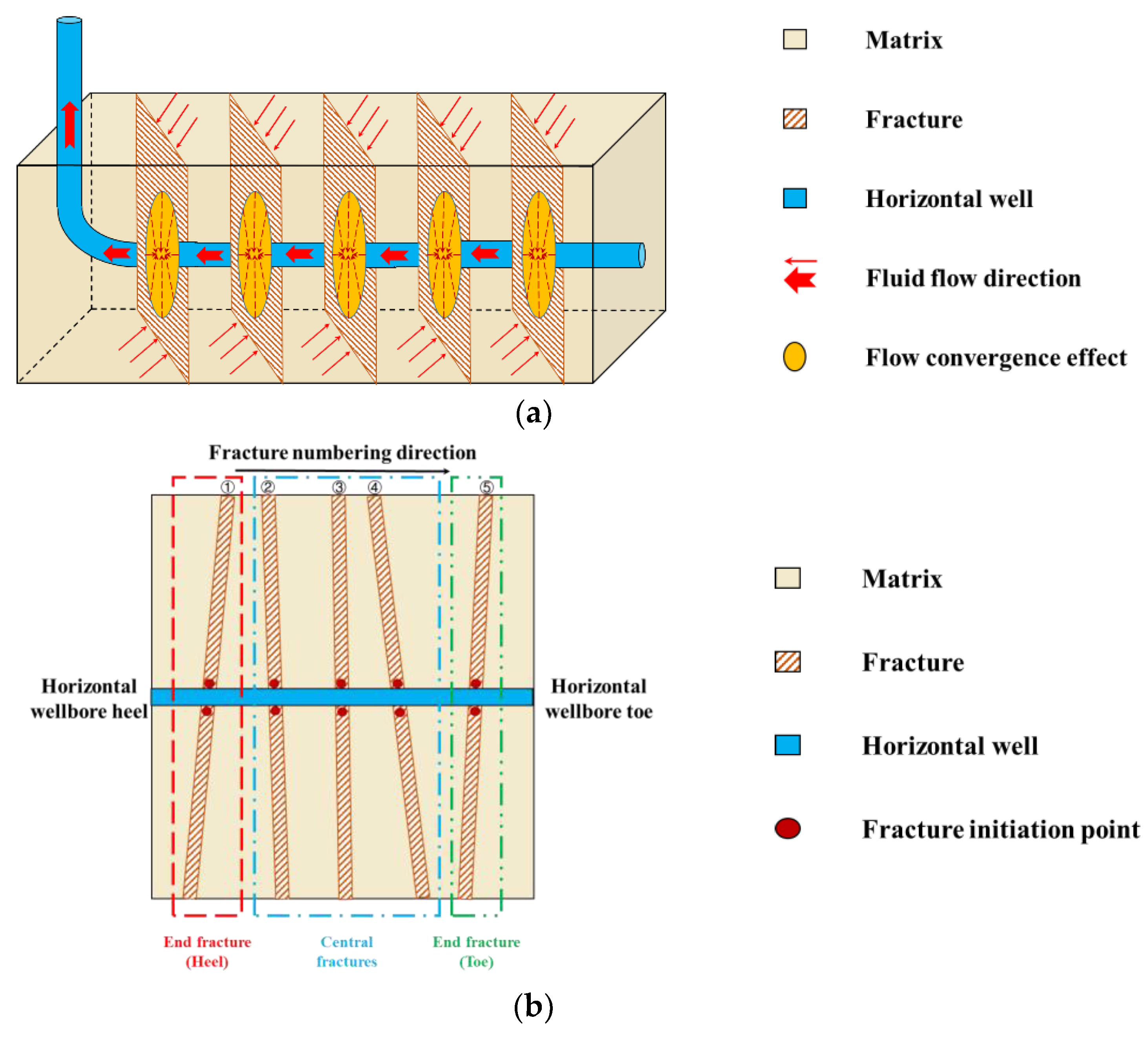
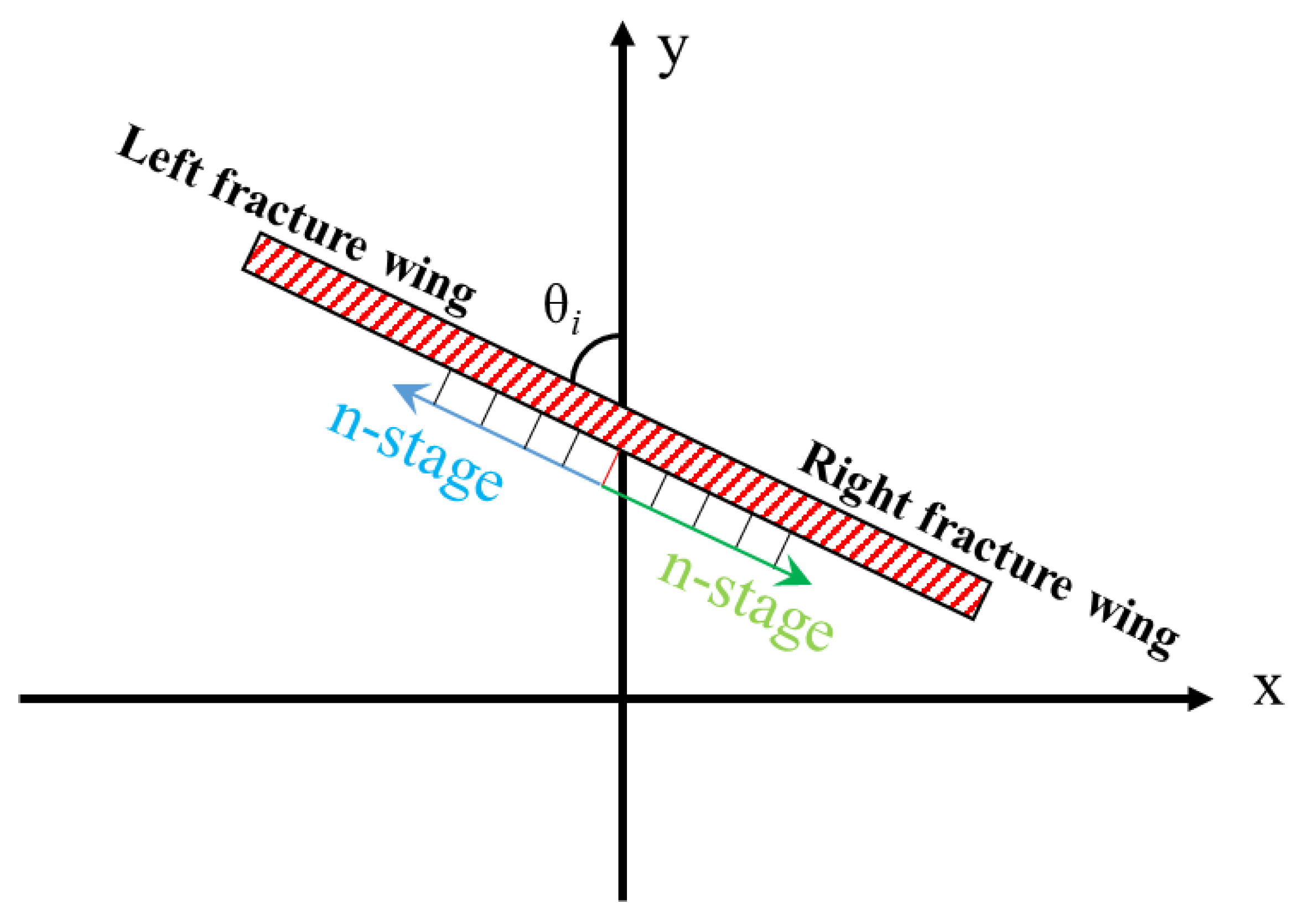
2.1. Physical Model and Assumptions

When reservoir formations are buried to certain depths, the vertical stress significantly exceeds horizontal stresses, leading hydraulic fractures to propagate perpendicular to the minimum principal stress direction, thus predominantly forming vertically oriented fractures. In most low-permeability reservoirs, post-fracturing operations reveal pronounced heterogeneity and poor pore-throat connectivity. Consequently, microfractures and pore channels within the matrix exhibit substantially lower seepage efficiency than hydraulic fractures—where fracture permeability exceeds matrix permeability by 10 to 10⁴ times or even orders of magnitude—justifying the neglect of direct matrix-to-wellbore fluid flow [27,28]. Furthermore, to achieve uniform fracture distribution and mitigate interference during production, diverting fracturing technology employing chemical diverters is routinely implemented. This technique redirects fluid flow within formations, controlling in-plane diversion or unidirectional fracture propagation, thus resulting in non-intersecting fractures propagating unidirectionally from initiation points [29]. Based on these assumptions, a triple-coupled matrix–fracture–wellbore physical model is established as illustrated in Figure 1a. Furthermore, as shown in Figure 1b, fractures are sequentially numbered from the horizontal wellbore heel (starting point) to the toe (endpoint). Fractures near the heel and toe are designated as end fractures, while others are categorized as central fractures.

The physical model for matrix–fracture–wellbore systems in fractured horizontal wells within low-permeability reservoirs is based on the following assumptions:

(1) The reservoir comprises a homogeneous, infinitely extended rectangular parallelepiped formation bounded by impermeable top and bottom strata, exhibiting negligible vertical flow, and the initial formation pressure corresponds to the average formation pressure; (2) Single-phase isothermal transient flow occurs within both reservoir and fractures, with capillary and gravitational forces excluded; (3) Fluid flow is segmented into three distinct stages: first from the matrix into fractures, then from fractures to the wellbore, and finally from the wellbore to surface production, disregarding direct connectivity between the matrix and wellbore; (4) All hydraulic fractures fully penetrate the reservoir vertically, with fracture heights matching formation thickness; (5) No hydraulic fractures intersect spatially.

2.2. Matrix–Fracture Flow Model

(1)

Pressure Drop Model at Any Point in the Matrix

The total production period is discretized into n infinitesimal computational segments, enabling oil production rates within each interval to be approximated as constant during numerical simulations [30]. Consequently, the matrix pressure drop within each interval can be approximated using the point-source pressure drop equation for a homogeneous infinite formation, expressed as follows:

$$\mathrm{\Delta }p\left(x,y,t\right)=p_i-p\left(x,y,t\right)={\displaystyle \frac{q\mu B}{4\pi K_{o}h}}\left[\ln {\displaystyle \frac{1}{\psi }}-0.5772+\psi -{\displaystyle \frac{{\psi }^2}{2\times 2!}}+{\displaystyle \frac{{\psi }^3}{3\times 3!}}-\dots +{(-1)}^{(n+1)}{\displaystyle \frac{{\psi }^2}{n\times n!}}\right]$$

(1)

where

$$\psi ={\displaystyle \frac{{\left(x-x_0\right)}^2+{\left(y-y_0\right)}^2}{4\eta t}}$$

(2)

$$K_o=V_k{\sigma }_k$$

(3)

where p_i is initial reservoir pressure, MPa; p(x, y, t) is formation pressure at point (x, y) at time t, MPa; q is volumetric flow rate at the point source, m³/s; (x₀, y₀) is point source coordinates; μ is reservoir oil viscosity, mPa·s; B is reservoir oil formation volume factor, dimensionless; K₀ is initial formation permeability, mD; V_k represents the coefficient of variation for reservoir permeability, quantifying the degree of permeability heterogeneity. A smaller value indicates stronger homogeneity, while a larger value corresponds to increased heterogeneity and this parameter is dimensionless; σ_k denotes the standard deviation of permeability and is likewise dimensionless; h is reservoir thickness, m; η is hydraulic diffusivity, m²·MPa/(MPa·s); and t is production time, s.

To simplify the formulation, we set the following:

$$\Re =\ln {\displaystyle \frac{1}{\psi }}-0.5772+\psi -{\displaystyle \frac{{\psi }^2}{2\times 2!}}+{\displaystyle \frac{{\psi }^3}{3\times 3!}}-\dots +{(-1)}^{(n+1)}{\displaystyle \frac{{\psi }^2}{n\times n!}}$$

(4)

Equation (1) can then be simplified as follows:

$$\mathrm{\Delta }p\left(x,y,t\right)=={\displaystyle \frac{q\mu B}{4\pi K_{o}h}}\Re$$

(5)

Given the low-porosity and low-permeability characteristics of low-permeability reservoirs, fluid flow deviates from steady-state Darcy’s law, primarily manifesting TPG and stress sensitivity effects. Incorporating TPG, the pressure drop equation becomes the following:

$$\mathrm{\Delta }p\left(x,y,t\right)-\lambda Gr={\displaystyle \frac{q\mu B}{4\pi K_{o}h}}\Re$$

(6)

where G is TPG, MPa/m, and λ is a dimensionless TPG correction factor, with a value range of 0 to 1.

Meanwhile, reservoir stress sensitivity affects the expansion of fractured joints and can even impact the stability of wellbore production [31]. The conventional stress-sensitive characterization equation is often obtained using the Terzaghi effective stress formula, which is not applicable to dense rocks and has a limited range of application. Conversely, the Biot modified effective stress formula can reflect different reservoir types or media using different Biot numbers, and it can be degraded to the stress-sensitive characterization equation obtained by Terzaghi effective stress [32]. The characterization equation is as follows:

$$K_p=K_0{\mathrm{e}}^{-{\alpha }_{\mathrm{k}}\beta (p_i-p)}$$

(7)

where K_p is represents matrix permeability under current pressure, mD; α_k is denotes the stress sensitivity coefficient, MPa⁻¹; β is the Biot coefficient (dimensionless, ranging from 0 to ~1); p is the current formation pressure, MPa.

Since the pressure at each point sink directly influences the current formation pressure and consequently affects matrix permeability, the pressure drop equation is reformulated as follows:

$$\mathrm{\Delta }p\left(x,y,t\right)-\lambda Gr={\displaystyle \frac{q\mu B}{4\pi K_{p}h}}\Re ={\displaystyle \frac{q\mu B}{4\pi K_0{\mathrm{e}}^{-{\alpha }_{\mathrm{k}}\beta (p_i-p)}h}}\Re$$

(8)

A Cartesian coordinate system is established with the horizontal well toe as the origin, where the y-axis aligns with the wellbore axis and the x-axis is perpendicular to it. The angle between fractures and the wellbore is designated as θ_i (0° ≤ θ_i ≤ 90°) (Figure 2). Each fracture wing is equidistantly divided into n segments. As n approaches infinity, each segment can be approximated by its centroid coordinates, thereby treating each subdivision as an independent point source.

Given the substantial volumetric dominance of horizontal wellbores over fractures in practical operations, the intersection of the i-th fracture with the wellbore is defined as its initiation point, with coordinates (0, y_i). Let L_i = L_li + L_ri be the total length of the i-th fracture, L_li the left wing length, and L_ri the right wing length.

The coordinates of the j-th point source on the left wing (negative direction) of the i-th fracture are given by Equation (9), where j = 1 corresponds to the left wing apex, written as follows:

$$\left(x_{ij},y_{ij}\right)=\left(-{\displaystyle \frac{1}{2}}\left({\displaystyle \frac{2n-2j+1}{n}}\right)L_{li}\sin {\theta }_i,y_i-{\displaystyle \frac{1}{2}}\left({\displaystyle \frac{2n-2j+1}{n}}\right)L_{li}\cos {\theta }_i\right)$$

(9)

Similarly, the coordinates of the j-th point source on the right wing (positive direction) of the i-th fracture are given by Equation (10), where j = 1 corresponds to the right wing apex, written as follows:

$$\left(x_{ij}^{\prime },y_{ij}^{\prime }\right)=\left({\displaystyle \frac{1}{2}}\left({\displaystyle \frac{2n-2j-1}{n}}\right)L_{ri}\sin {\theta }_i,y_i-{\displaystyle \frac{1}{2}}\left({\displaystyle \frac{2n-2j-1}{n}}\right)L_{ri}\cos {\theta }_i\right)$$

(10)

Substituting the coordinates of the j-th point source on both wings of the i-th fracture into Equation (8) and applying the potential superposition principle, the cumulative pressure drop at time t induced by the i-th fracture at any location is as follows:

$$\left(\mathrm{\Delta }p(x,y,t)-\lambda Gr\right){|}_i=\sum _{j=1}^n{\displaystyle \frac{q_{ij}\mu B}{4\pi K_0{\mathrm{e}}^{-{\alpha }_{\mathrm{k}}\beta (p_i-p)}h}}{\Re }_{ij}+\sum _{j=1}^n{\displaystyle \frac{q_{ij}^{\prime }\mu B}{4\pi K_0{\mathrm{e}}^{-{\alpha }_{\mathrm{k}}\beta (p_i-p)}h}}{\Re }_{ij}^{\prime }$$

(11)

where

$$\left\{\begin{array}{l}{\psi }_{ij}={\displaystyle \frac{{\left(x-x_{ij}\right)}^2+{\left(y-y_{ij}\right)}^2}{4\eta t}}\\ {\psi }_{ij}^{\prime }={\displaystyle \frac{{\left(x-x_{ij}^{\prime }\right)}^2+{\left(y-y_{ij}^{\prime }\right)}^2}{4\eta t}}\end{array}\right.$$

(12)

Integrating the pressure drop equations for both wings of a single fracture yields the total pressure drop at any point (x, y) in the formation matrix at time t when m fractures produce simultaneously, written as follows:

$$\left(\mathrm{\Delta }p(x,y,t)-\lambda Gr\right){|}_m={\displaystyle \sum _{i=1}^m\left\{\sum _{j=1}^n\frac{q_{ij}\mu B}{4\pi K_0{\mathrm{e}}^{-{\alpha }_{\mathrm{k}}\beta (p_i-p)}h}{\Re }_{ij}+\sum _{j=1}^n\frac{q_{ij}^{\prime }\mu B}{4\pi K_0{\mathrm{e}}^{-{\alpha }_{\mathrm{k}}\beta (p_i-p)}h}{\Re }_{ij}^{\prime }\right\}}$$

(13)

where m is the total number of fractures; q_ij is the oil production rate at the j-th point on the left wing of the i-th fracture, m³/d; and q_ij′ represents the rate at the corresponding right-wing point, m³/d.

(2)

Matrix–Fracture Flow Model

Substituting the left-wing apex coordinates (x_lki, y_lki) of the i-th fracture into Equation (13), the pressure drop between all point sources and the left-wing apex at time t under simultaneous production from m fractures is written as follows:

$$\left(p_i-p_{li}-\lambda Gr\right){|}_{\mathrm{m}}=\sum _{k=1}^{\mathrm{m}}\left\{\sum _{j=1}^n{\displaystyle \frac{q_{lij}\mu B}{4\pi K_0{\mathrm{e}}^{-{\alpha }_{\mathrm{k}}\beta (p_i-p)}h}}{\Re }_{lki}+\sum _{j=1}^n{\displaystyle \frac{q_{lij}^{\prime }\mu B}{4\pi K_0{\mathrm{e}}^{-{\alpha }_{\mathrm{k}}\beta (p_i-p)}h}}{\Re }_{lki}^{\prime }\right\}$$

(14)

where p_li is the pressure at the left-wing apex of the i-th fracture, Pa; (x_ki, y_ki) is the coordinates of the j-th point source on the left wing of the k-th fracture, and (x_ki′, y_ki′) corresponds to the right-wing point source.

Similarly, substituting the right-wing apex coordinates into Equation (13) yields the following:

$$\left(p_i-p_{ri}-\lambda Gr\right){|}_{\mathrm{m}}=\sum _{k=1}^{\mathrm{m}}\left\{\sum _{j=1}^n{\displaystyle \frac{q_{rij}\mu B}{4\pi K_0{\mathrm{e}}^{-{\alpha }_{\mathrm{k}}\beta (p_i-p)}h}}{\Re }_{rki}+\sum _{j=1}^n{\displaystyle \frac{q_{rij}^{\prime }\mu B}{4\pi K_0{\mathrm{e}}^{-{\alpha }_{\mathrm{k}}\beta (p_i-p)}h}}{\Re }_{rki}^{\prime }\right\}$$

(15)

Given the equidistant fracture distribution and infinite homogeneous formation, the apex pressure of each fracture can be approximated as the average of its left- and right-wing apex pressures. Combining Equations (14) and (15), the equilibrium pressure equation at time t for all point sources across m fractures is established as follows:

$$p\left(x_i,y_i,t\right)={\displaystyle \frac{p_{li}+p_{ri}}{2}}=p_i-\lambda Gr=-{\displaystyle \frac{1}{2}}\left\{\begin{array}{l}{\displaystyle \sum _{k=1}^{\mathrm{m}}}\left[{\displaystyle \sum _{j=1}^n}{\displaystyle \frac{q_{lij}\mu B}{4\pi K_0{\mathrm{e}}^{-{\alpha }_{\mathrm{k}}\beta (p_i-p)}h}}{\Re }_{lki}+{\displaystyle \sum _{j=1}^n}{\displaystyle \frac{q_{lij}^{\prime }\mu B}{4\pi K_0{\mathrm{e}}^{-{\alpha }_{\mathrm{k}}\beta (p_i-p)}h}}{\Re }_{lki}^{\prime }\right]\\ +{\displaystyle \sum _{k=1}^{\mathrm{m}}}\left[{\displaystyle \sum _{j=1}^n}{\displaystyle \frac{q_{rij}\mu B}{4\pi K_0{\mathrm{e}}^{-{\alpha }_{\mathrm{k}}\beta (p_i-p)}h}}{\Re }_{rki}+{\displaystyle \sum _{j=1}^n}{\displaystyle \frac{q_{rij}^{\prime }\mu B}{4\pi K_0{\mathrm{e}}^{-{\alpha }_{\mathrm{k}}\beta (p_i-p)}h}}{\Re }_{rki}^{\prime }\right]\end{array}\right\}$$

(16)

Let the oil production rate of the i-th fracture be q_i, with all fluid uniformly influxing from the matrix along the fracture plane. The production rates of the left and right wings of the i-th fracture can be expressed proportionally to their respective lengths, written as follows:

$$q_{li}={\displaystyle \frac{L_{li}}{L_i}}{q}_i$$

(17)

$$q_{ri}={\displaystyle \frac{L_{ri}}{L_i}}{q}_i$$

(18)

where q_li and q_ri denote the production rates of the left and right wings of the i-th fracture, respectively, m³/d.

When the left and right wings are symmetric (L_li = L_ri = L_(s) = L_i/2), and each fracture is divided into n equal segments, the number of subdivisions per wing becomes n/2. Assuming identical production rates for all point sinks on both wings and it is q_i(s), we derive the following:

$$q_i(s)=q_{li}=q_{ri}={\displaystyle \frac{q_i}{2n{L}_i}}$$

(19)

The pressure drop model at any point in the matrix is thus simplified as follows:

$$\begin{array}{ll}\hfill \mathrm{\Delta }p\left(x_i,y_i,t\right)-\lambda Gr& =-{\displaystyle \sum _{k=1}^{\mathrm{m}}}\left[{\displaystyle \sum _{j=1}^n}{\displaystyle \frac{q_{ki}(s)\mu B}{4\pi K_0{\mathrm{e}}^{-{\alpha }_{\mathrm{k}}\beta (p_i-p)}h}}{\Re }_{ij}+{\displaystyle \sum _{j=1}^n}{\displaystyle \frac{q_{ki}(s)\mu B}{4\pi K_0{\mathrm{e}}^{-{\alpha }_{\mathrm{k}}\beta (p_i-p)}h}}{\Re }_{ij}^{\prime }\right]\hfill \\ & =-{\displaystyle \sum _{k=1}^{\mathrm{m}}}\left[{\displaystyle \sum _{j=1}^n}{\displaystyle \frac{q_{ki}\mu B}{8\pi n{K}_0{\mathrm{e}}^{-{\alpha }_{\mathrm{k}}\beta (p_i-p)}h{L}_i}}\left({\Re }_{ij}+{\Re }_{ij}^{\prime }\right)\right]\hfill \end{array}$$

(20)

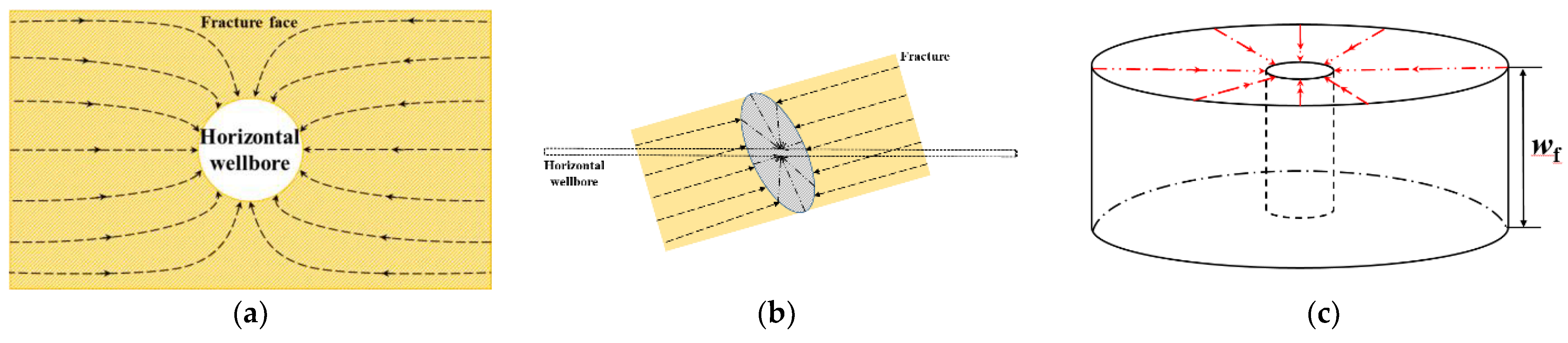
2.3. Fracture–Wellbore Flow Model

Compared with low-permeability formations, fractures generally have much higher conductivity. The flow process in the fracture–wellbore system can be divided into two stages: linear flow within the fracture away from the wellbore and radial flow in the near-wellbore region. Due to fluid flow within the fracture, the TPG need not be considered. However, as reservoir pressure declines, the effective stress increases, causing the proppant within the fracture to gradually fail and the fracture to progressively close. Consequently, the stress sensitivity of the fracture must be accounted for. In the coupled flow analysis of the artificial fracture system and the wellbore system, given the premise that the fracture possesses the structural characteristic of fully penetrating the formation layer, and considering that its half-length parameter holds orders of magnitude advantage relative to both the vertical scale of the reservoir and the radial dimension of the wellbore, the seepage process of crude oil flowing from the fracture edge into the horizontal wellbore can be simplified to a planar radial flow mode under the condition of neglecting the effects of gravity and capillary forces, as illustrated in Figure 3.

Therefore, based on the above analysis of fluid flow in the fracture–wellbore system, the following preconditions are specified:

(1) The boundary pressure for the fracture–wellbore flow model is the endpoint pressure p(x_i, y_i, t) at the top of the i-th fracture. (2) The pressure at the initiation point of the i-th crack is p_wfi, and the pressure at the initiation point of the (i − 1)-th crack is p_wf(i-1). (3) The effective reservoir thickness is taken equal to the width of the i-th fracture w_f. (4) The flow area is taken equal to the fracture area.

$$R_i=\sqrt{{\displaystyle \frac{\left(L_{li}+L_{ri}\right)h}{\pi }}}=\sqrt{{\displaystyle \frac{L_{i}h}{\pi }}}=\sqrt{{\displaystyle \frac{A_f}{\pi }}}$$

(21)

where A_f is the effective drainage area of the fracture, m².

Consequently, the fluid flow process from the i-th fracture to the horizontal wellbore can be described as an equivalent microscale planar radial flow process, written as follows:

$$p\left(x_i,y_i,t\right)-p_{wfi}={\displaystyle \frac{q_{fi}\mu B}{2\pi K_f{w}_{fi}}}\ln \left({\displaystyle \frac{R_i}{r_w}}+S_c\right)$$

(22)

where q_fi is the production rate of the i-th fracture, m³/s; k_i is the permeability of the i-th fracture, mD; w_fi is the width of the i-th fracture, m; h is the reservoir thickness, m; S_c is the fracture convergence skin factor; and r_w is the radius of the horizontal wellbore, m.

Considering stress sensitivity effects in hydraulic fractures, we obtain the following:

$$K_f=K_{fo}{\mathrm{e}}^{-{\alpha }_k\beta (p_i-p)}$$

(23)

where k_f is the fracture permeability under current pressure, mD, and k_fo is the initial fracture permeability, mD.

By combining Equation (20) with Equation (22), the total pressure drop equation for the i-th fracture can be derived. This equation comprehensively accounts for pressure losses occurring both in the matrix–fracture interaction and the fracture–wellbore flow pathway.

$$p_i-p_{wfi}-\lambda Gr=\begin{array}{c}-{\displaystyle \sum _{k=1}^{\mathrm{m}}}\left[{\displaystyle \sum _{j=1}^n}{\displaystyle \frac{q_{ki}\mu B}{8\pi n{K}_0{\mathrm{e}}^{-{\alpha }_{\mathrm{k}}\beta (p_i-p)}h{L}_i}}\left({\Re }_{ij}+{\Re }_{ij}^{\prime }\right)\right]+{\displaystyle \frac{q_{fi}\mu B}{2\pi K_{fi}{w}_{fi}}}\ln \left({\displaystyle \frac{R_i}{r_w}}+S_c\right)\end{array}$$

(24)

Considering inter-fracture interference effects, the skin factor S_c can be determined using the following expression:

$$S_{\mathrm{c}}={\displaystyle \frac{Kh}{K_{fi}{w}_{f\mathrm{i}}}}\left(\ln \left({\displaystyle \frac{h}{2r_{\mathrm{w}}}}\right)-{\displaystyle \frac{\pi }{2}}\right)={\displaystyle \frac{Kh}{K_{foi}{\mathrm{e}}^{-{\alpha }_{\mathrm{k}}\beta (p_i-p)}{w}_{f\mathrm{i}}}}\left(\ln \left({\displaystyle \frac{h}{2r_{\mathrm{w}}}}\right)-{\displaystyle \frac{\pi }{2}}\right)$$

(25)

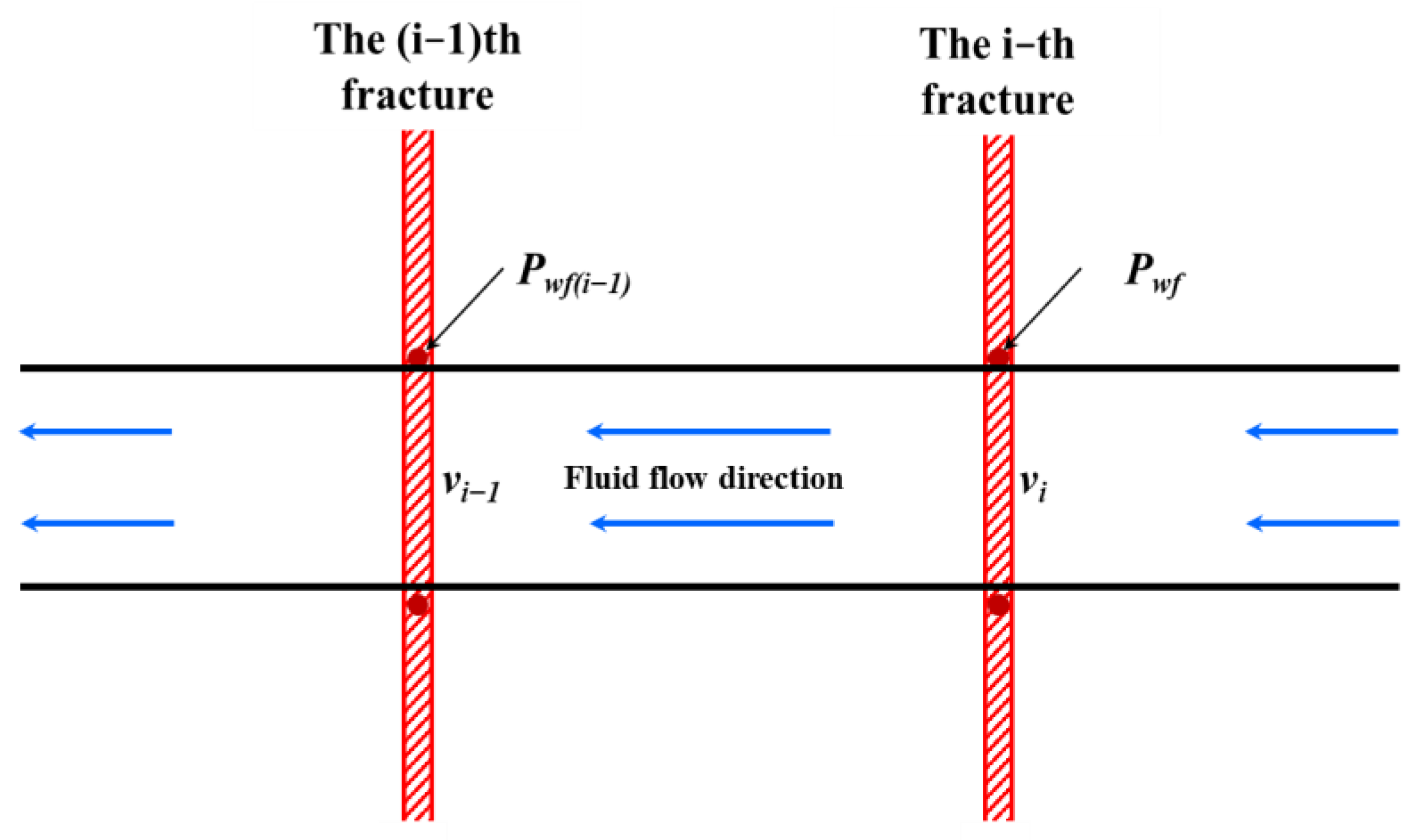
2.4. Wellbore Fluid Flow Model

Fluid inflow from fractures into the wellbore incurs measurable pressure losses due to wellbore friction and flow convergence effects, substantially impacting actual productivity in fractured horizontal wells. Utilizing the aforementioned coordinate system, we analyze pressure drop behavior within the wellbore.

Similarly, the wellbore segment between the i-th and (i − 1)-th fractures (designated as segment k where k = 1, 2, …, m) is analyzed as shown in Figure 4. The fluid influx velocity from the i-th fracture into the wellbore is v_i, decreasing to velocity v_i-1 at the (i − 1)-th fracture. Consequently, the wellbore pressure drop between these fractures comprises frictional losses and acceleration-induced components.

The shear stress exerted on the wellbore wall induces frictional pressure losses in the fluid flow. This frictional component is calculated as follows:

$$\mathsf{\Delta }{p}_{w\mathrm{i}}=p_{wfi}-p_{wf(i-1)}={\displaystyle \frac{{\tau }_{wk}\pi D\left(y_i-y_{i-1}\right)}{A}}={\displaystyle \frac{f_k\rho v_k^2\left(y_i-y_{i-1}\right)}{4r_w}}$$

(26)

$${\tau }_{wk}={\displaystyle \frac{f_k\rho v_k^2}{8}}$$

(27)

where τ_wk is the shear stress on the wellbore wall, MPa; D is the wellbore diameter, m; f_k is the friction coefficient of the k-th section of the wellbore wall, dimensionless; ρ is the density of crude oil, g/m³; A is the wellbore cross-sectional area, m²; v_k is the fluid velocity in the k-th section of the wellbore, m/s.

At the same time, we obtain the following:

$$v_k={\displaystyle \frac{q_k}{A}}={\displaystyle \frac{q_k}{\pi r_w^2}}$$

(28)

$$\left\{\begin{array}{l}{q}_k=q_{fi}+q_{f(i+1)}(k=1,2,\dots ,m-1)\\ q_k=q_{fi}(k=m)\end{array}\right.$$

(29)

where q_k is the flow rate of the fluid in the k-th wellbore segment, m³/s.

Substituting Equation (28) into Equation (26) yields the following:

$$\mathsf{\Delta }{p}_{w\mathrm{i}}={\displaystyle \frac{{\tau }_{wk}\pi D\left(y_i-y_{i-1}\right)}{A}}={\displaystyle \frac{f_k\rho q_k^2\left(y_i-y_{i-1}\right)}{4\pi r_w^5}}$$

(30)

The friction coefficient of the k-th section of the wellbore wall is given by the following:

$$\left\{\begin{array}{l}{f}_k={\displaystyle \frac{64}{R{e}_k}}\left({\mathrm{Re}}_k\le 2000\right)\\ {\displaystyle \frac{1}{\sqrt{f_k}}}=1.14-2\ln \left({\displaystyle \frac{e}{2r_w}}+{\displaystyle \frac{21.25}{R{e}_k^{0.9}}}\right)\left(R{e}_k\ge 4000\right)\end{array}\right.$$

(31)

where

$$R{e}_k={\displaystyle \frac{2\rho v_k{r}_w}{\mu }}={\displaystyle \frac{2\rho q_k}{\mu \pi r_w}}$$

(32)

where e is the absolute roughness of the wellbore wall, m, and R_ek is the Reynolds number for the k-th wellbore segment, used to determine the fluid flow regime within this segment.

The flow regime is laminar when Re ≤ 2000, turbulent when Re ≥ 4000, and transitional when 2000 < Re < 4000. In actual production scenarios, constrained by reservoir properties and drilling technology limitations, the flow regime in the wellbore is predominantly transitional. Therefore, f_k is calculated as the weighted average of the laminar and turbulent flow values.

$$f_k=ƛf_1+(1-ƛ)f_2$$

(33)

where f₁ and f₂ are the friction coefficients for laminar and turbulent flow, respectively, dimensionless; and $ƛ$ is the weighting ratio between the two, typically ranging from 0.1 to 0.3.

During the production process of horizontal fracturing wells, fluid continuously flows into the wellbore through the fractures. This leads to an increase in fluid mass within the wellbore, causing an acceleration pressure drop. Since fluid only flows into the wellbore through the fractures under the aforementioned assumptions, the acceleration pressure drop occurs exclusively at the fractures, yielding the following equation:

$$\left\{\begin{array}{l}\mathsf{\Delta }{p}_{\alpha i}=\rho \left({\nu }_{(i-1)}^2-{\nu }_i^2\right)={\displaystyle \frac{\rho \left(q_k^2-q_{(k+1)}^2\right)}{{\pi }^2{r}_w^4}}(i=1,2,\dots ,m-1)\\ \mathsf{\Delta }{p}_{\alpha i}=0(i=m)\end{array}\right.$$

(34)

At the same time, since the width of the fracture is much smaller than that of the wellbore, and since the acceleration pressure drop only occurs at the fracture, the acceleration pressure drop of the i-th fracture can be approximated as the average value of the acceleration pressure drop.

$$\mathsf{\Delta }{p}_{\alpha fi}={\displaystyle \frac{1}{2}}\mathsf{\Delta }{p}_{\alpha i}$$

(35)

Therefore, the pressure p at the bottom of the i-th fracture is obtained as follows:

$$\left\{\begin{array}{l}{p}_{wfi}=p_{wf1}+\mathsf{\Delta }{p}_{w1}+\mathsf{\Delta }{p}_{afi}\left(i=1\right)\\ p_{wfi}=p_{wf(i-1)}+\mathsf{\Delta }{p}_{wi}+\left[\mathsf{\Delta }{p}_{af(i-1)}+\mathsf{\Delta }{p}_{afi}\right]\left(i=2,3,\dots ,m\right)\end{array}\right.$$

(36)

Finally, since only the inflow of formation fluid into the wellbore through the fractures is considered and not the direct inflow of fluid from the matrix, according to the law of mass conservation, the total production of the entire fractured horizontal well is the sum of the productions of all the fractures. Solving Equations (24) and (36) simultaneously determines the production of each fracture. Assuming there are m fractures, the production of the fractured horizontal well is written as follows:

$$Q={\displaystyle \sum _{i=1}^m{q}_i}$$

(37)

To improve computational efficiency, this study employs Python programming and solves the model in MATLAB^® software R2023b. The specific solution procedure is illustrated in Figure 5.

3. Model Validation

Existing productivity prediction models for fractured horizontal wells each possess specific applicability conditions. Considering both the parameter acquisition context in this study and model relevance, the horizontal well productivity prediction model from Reference [15] can serve as the validation benchmark (It was subsequently referred to as the comparison model).

Table 1. Reservoir and fractured horizontal well parameters in an offshore oilfield.

Parameter Name	Value	Parameter Name	Value
Reservoir Thickness1/2, m	25/33.5	Wellbore Radius, m	0.1
Formation Permeability1/2, mD	1.5/14.4	Fracture Width, m	0.005
Formation Porosity1/2, %	12/15.8	Angle between Fracture and Horizontal Well, °	90
Compressibility Coefficient, MPa−1	8 × 10−5	TPG Coefficient1/2	0.82/0.53
Formation Pressure1/2, MPa	29.05/45.34	TPG1/2, MPa/m	0.005/0.003
Bottomhole Flowing Pressure1/2, MPa	19.05/25.34	Number of Fractures	6
Horizontal Well Length1/2, m	400/500	Fracture Half-Length, m	100
Crude Oil Viscosity1/2, mPa·s	1.29/0.21	Fracture Permeability, mD	100
Density of Crude Oil, g/cm3	0.68/0.59	Biot Number	0.8
Volume Coefficient1/2	1.34/1.84	Matrix Stress Sensitivity Coefficient1/2, MPa−1	0.02/0.01
Absolute Roughness of the Wellbore Wall	0.00002	Fracture Stress Sensitivity Coefficient, MPa−1	0.01

presents fundamental parameters for two distinct offshore reservoir blocks and their corresponding fractured horizontal wells (differing values for identical parameters are distinguished as Parameter1/Parameter2). These basic parameters are substituted into the production capacity prediction model and the comparison model, and the production capacity of the horizontal well and the production capacity of each fracture along the horizontal well are calculated. The calculated production capacity is then compared with the actual production capacity of the well (due to the difficulties in production and development of offshore oilfields, relevant initial production test data cannot be provided stably, so the actual production data within 360 days after production stabilization is used as the actual production capacity of the well). The datasets for the two wells are designated as Horizontal Well 1 and Horizontal Well 2, respectively.

Figure 6 demonstrates that the overall model’s calculated productivity consistently exceeds actual values. This discrepancy primarily arises from the substantial heterogeneity in the actual low-permeability reservoir and the complex seepage dynamics of formation fluids, leading to theoretical model outputs exceeding field production data. Furthermore, since the benchmark models fail to account for wellbore fluid pressure losses, this results in overestimated productivity predictions for the fractured horizontal wells in both reservoir blocks. Although the present model exhibits minor deviations from actual production during initial stages, it achieves strong alignment with field productivity during mid-to-late stages. Notably, Horizontal Well 2 experienced a decline in production capacity due to an insufficient energy supply during actual production. This resulted in significant fluctuations in production data during the mid-term period and poor agreement between the model’s calculated results and actual data during that time. The overall average error between the model’s results and the actual production data was 6.98% for Horizontal Well 1 and 5.87% for Horizontal Well 2, indicating small errors and confirming the accuracy and reliability of the model.

Table 2. Computed productivity of individual fractures along the horizontal well.

Horizontal Well Zone	Fracture-Contributed Production (m3/d)							Fieldwide Total Production (m3/d)	Actual Production (m3/d)
	Fracture ID	1	2	3	4	5	6
Horizontal well 1	The comparison model	9.28	8.87	8.69	8.70	8.89	9.26	53.69	44.3
	The proposed model	9.65	8.87	7.05	6.8	8.05	9.43	49.85
Horizontal well 2	The comparison model	15.03	14.93	14.89	14.91	14.91	15.06	89.73	77.74
	The proposed model	14.9	13.98	12.98	13.06	14.04	14.9	83.86

presents calculated productivity values for individual fractures distributed along the horizontal well, using Day 1 daily oil production as the representative case. The modeling results reveal higher production from fractures near the well extremities and lower output from mid-well fractures. This distribution pattern arises from fracture interference due to competitive propagation during hydraulic fracturing. Notably, the comparison model calculates uniformly higher fracture productivities while exhibiting wider production differentials between fractures—particularly between terminal and central fractures. However, actual production data demonstrates that fracture interference typically yields less pronounced productivity variations. This overestimation of differentials constitutes a primary factor in the comparison model’s significant overprediction of total productivity. Conversely, the present model generates narrower productivity differentials among fractures, resulting in total production predictions that align closely with actual values. This consistency provides further compelling validation of the model’s accuracy and reliability.

4. Sensitivity Analysis of Productivity Influencing Factors

Based on the reservoir parameters provided in Table 1 (Take the relevant parameters of oil reservoir block 1 as an example.), the established productivity model for fractured horizontal wells was utilized to conduct sensitivity analysis on key productivity-influencing factors, primarily including reservoir characteristics (TPG and stress sensitivity coefficients) and fracture characteristics (fracture half-length and number of fractures).

4.1. Threshold Pressure Gradient

By exclusively varying the TPG while maintaining other parameters constant, the influence of this factor on fractured horizontal well productivity under different drawdown pressures was systematically analyzed. Figure 7 presents the resulting daily oil production curves of the fractured horizontal well and the comparative productivity profiles of individual fractures along the wellbore under a 10 MPa drawdown pressure.

As shown in Figure 7, the TPG significantly impacts the production capacity of horizontal fractured wells. As the initial pressure gradient increases, the overall production capacity of the horizontal well and the production capacity of each fracture gradually decrease at an increasing rate. When G ≤ 0.01 MPa/m, the average production decline rates for the two production pressure differentials are 11.62% (production pressure differential of 5 MPa) and 6.36% (production pressure differential of 10 MPa), respectively. When G > 0.01 MPa/m, the respective average production decline rates were 62.08% and 14.15%. This is primarily because the initial pressure gradient affects fluid flow conditions: the greater the pressure gradient, the greater the fluid flow resistance and the more difficult the flow becomes. Additionally, as Figure 7b shows, when the initial pressure gradient is large, most of the production from a horizontal well originates from the fractures at both ends of the well. The difference in production capacity between the central fracture and the end fractures also increases significantly (e.g., Fractures 1 and 3). Furthermore, when the production pressure differential is 10 MPa, the horizontal well’s daily oil production is, on average, 22.41 m³/d higher than when the production pressure differential is 5 MPa, representing an average reduction of 26.59%. Clearly, increasing the production pressure differential can effectively mitigate the adverse effects of the initial pressure gradient on horizontal well production.

4.2. Stress Sensitivity Coefficients

By independently varying stress sensitivity coefficients (categorized into matrix and fracture stress sensitivity coefficients, with one parameter altered while the other remained constant as per Table 1), the daily oil production curves of the fractured horizontal well and comparative productivity profiles of individual fractures along the wellbore (using fracture stress sensitivity coefficient variations as an example) were obtained, as illustrated in Figure 8.

The production of the fractured horizontal well decreases with increasing stress sensitivity coefficients, with distinct impacts observed between matrix and fracture stress sensitivity effects. The matrix stress sensitivity coefficient exhibits a relatively minor influence, causing an average production decline of 1.92 m³/d (4.32% reduction). In contrast, the fracture stress sensitivity coefficient significantly impacts productivity, resulting in an average production drop of 4.87 m³/d (20.93% reduction), with more pronounced declines observed in individual fracture contributions.

This disparity fundamentally stems from the limited effective flow pathways within the low-permeability reservoir matrix system, whereas hydraulic fractures dominate as preferential conduits for oil migration toward the wellbore. During production, continuous increases in effective stress induce progressive fracture closure, leading to geometric compression of preferential flow channels and dynamic attenuation of conductivity. This permeability degradation, driven by geomechanical damage mechanisms, exhibits an irreversible nature. Therefore, the production of the same fracture varies significantly under different fracture stress sensitivity coefficients, especially for fractures located at both ends (e.g., the average production difference for Fracture 1 is 3.37 m³/d). This demonstrates that stress sensitivity constitutes a critical influencing factor that cannot be neglected in the productivity evaluation of horizontal wells in low-permeability reservoirs.

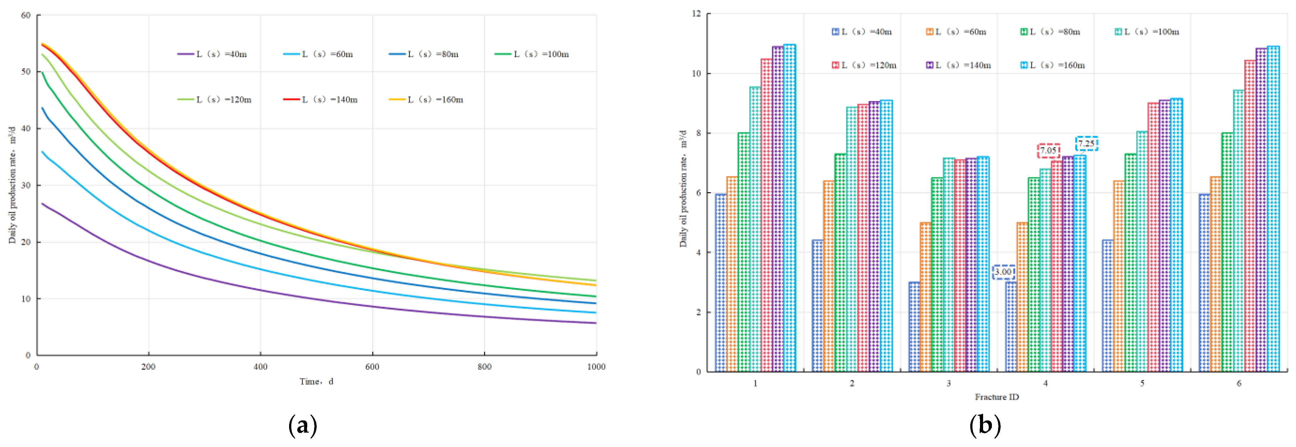
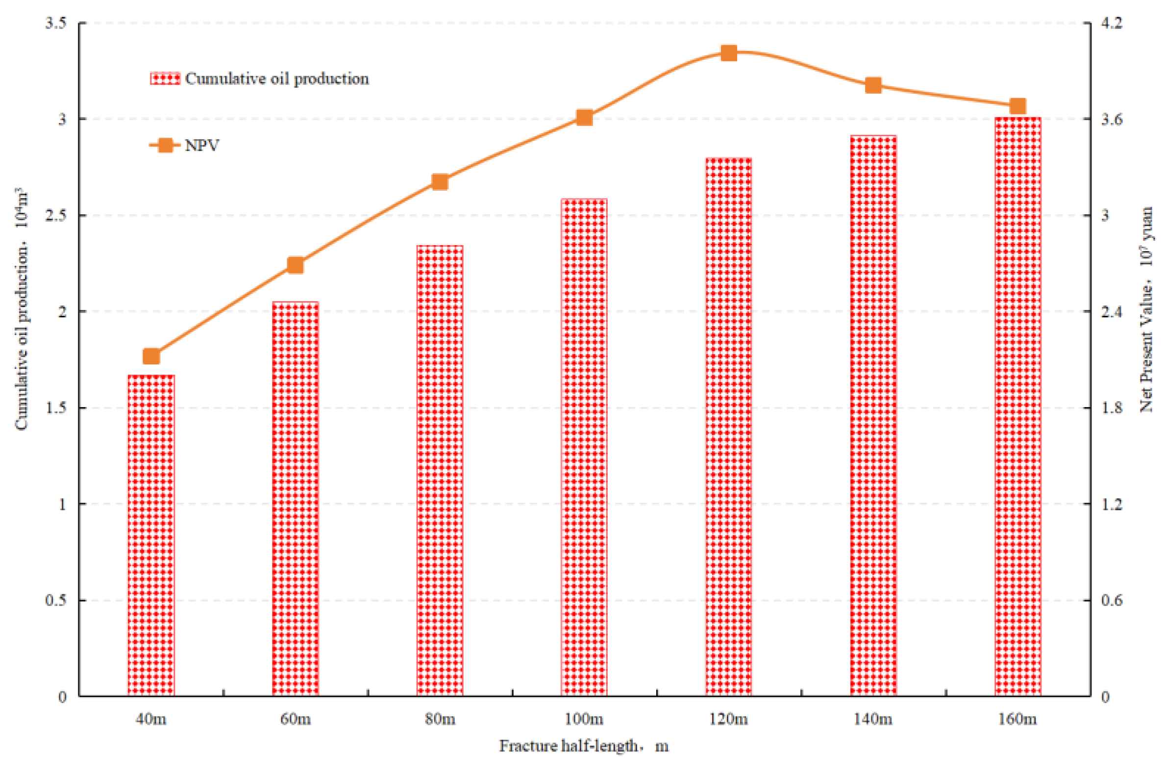
4.3. Fracture Half-Length

By exclusively varying fracture half-length while maintaining other parameters constant and incorporating transient flow behavior characteristic of actual horizontal well production, the productivity evolution of the fractured horizontal well was analyzed over a continuous operational period. Figure 9 presents the daily oil production curves and comparative productivity profiles of individual fractures along the wellbore (using Day 1 production rates under varying fracture half-lengths as an example).

Overall, the productivity of horizontal wells increases with fracture half-length, exhibiting a positive relationship. When the fracture half-length is small (L(s) ≤ 100 m), increasing the fracture half-length significantly enhances the overall productivity of horizontal wells, with an average increase reaching 21.61%. For individual fractures, taking Fracture 4 as an example, the maximum production increase reaches 4.05 m³/d. However, when the fracture half-length exceeds a certain threshold (L(s) > 100 m)—where fractures exhibit finite conductivity due to limitations in reservoir properties and fracturing techniques—the productivity enhancement effect of fracture half-length diminishes. The overall average increase is only 7.1%, and the production increase for individual fractures decreases even more markedly, with this effect being most pronounced for central fractures (again taking Fracture 4 as an example, the maximum production increase is merely 0.2 m³/d). As production progresses into the decline phase, large-scale artificial fractures experience closure under the dual effects of proppant performance degradation and in situ stress field reconfiguration, leading to geometric contraction of preferential flow paths.

During the production decline phase, large-scale hydraulic fractures undergo closure due to the combined effects of proppant performance degradation and in situ stress field redistribution, leading to geometric contraction of dominant flow pathways. Consequently, wells with initially high-production long fractures experience accelerated late-stage productivity declines. Furthermore, excessively long fractures escalate investment costs and technical demands, necessitating optimization of fracture half-length in low-permeability reservoirs to balance economic viability with production efficiency.

Taking into account the economic factors that oilfield companies must consider during production, such as drilling investments, fracturing costs, and sales profits, the net present value (NPV) method was used to analyze the relationship between fracture half-length and the technical–economic balance. The NPV analysis results are presented in Figure 10. There is a positive correlation between the cumulative oil yield and the fracture half-length, but the NPV shows that the fracture half-length has a limiting optimal value, which shows a trend of first increasing and then decreasing. A comprehensive techno-economic evaluation reveals that the technical optimum occurs at L(s) = 160 m, corresponding to maximum reservoir production, whereas the economic optimum is achieved at L(s) = 120 m, where NPV reaches its peak values. Consequently, the reservoir attains optimal cost–benefit equilibrium at L(s) = 120 m through integrated modeling and economic analysis.

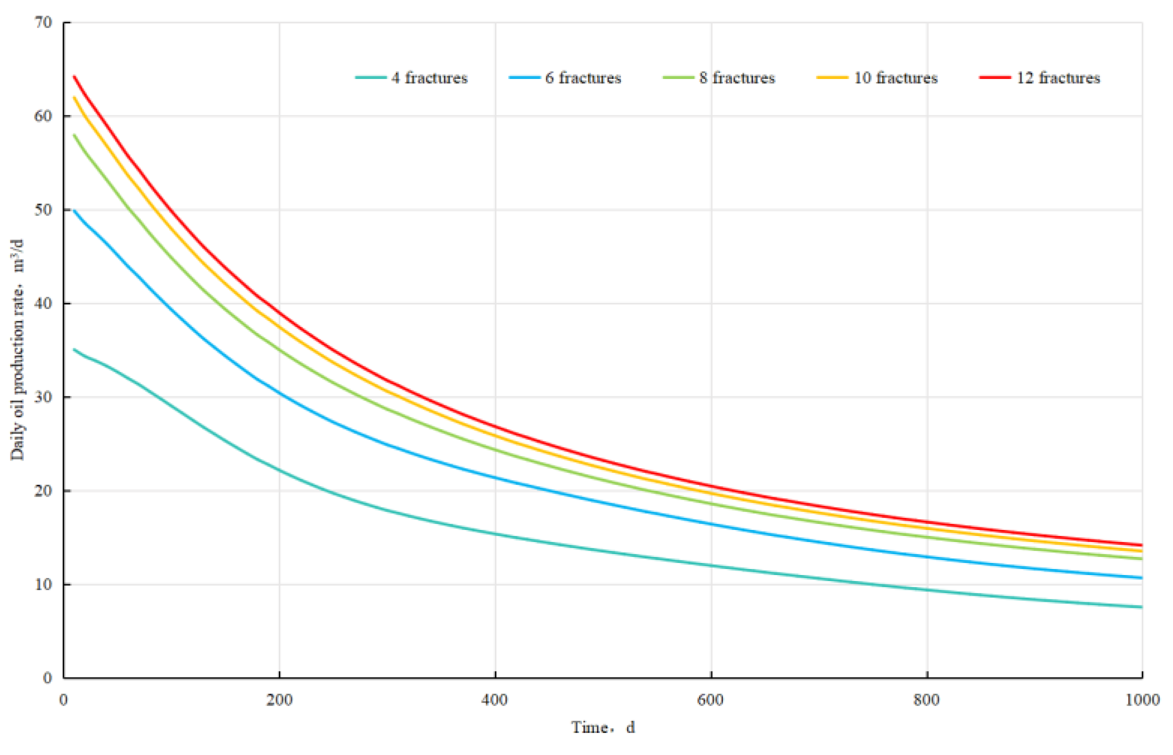
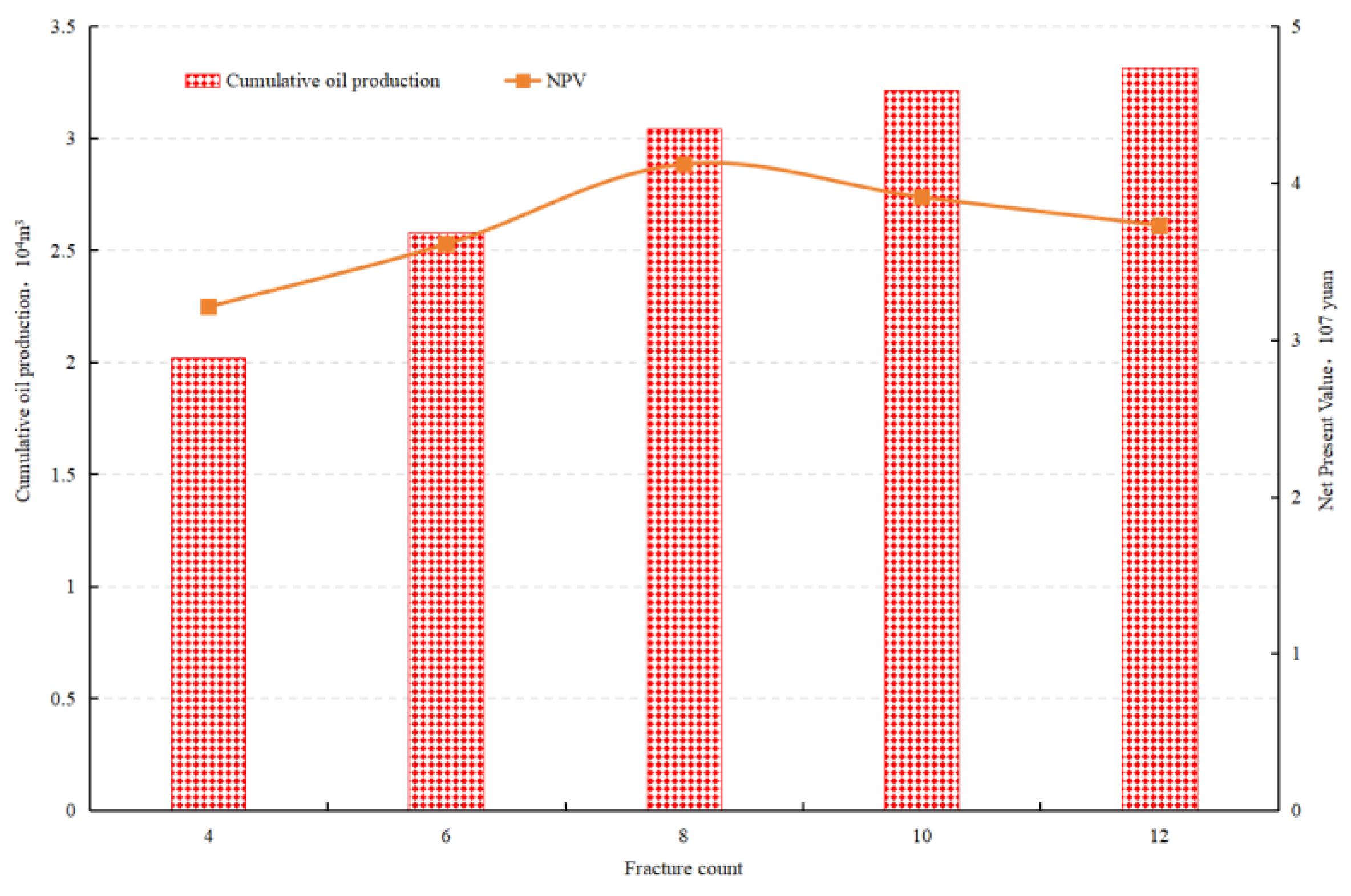
4.4. Number of Fractures

By exclusively varying the number of fractures while maintaining other parameters constant, the productivity response of the fractured horizontal well was systematically investigated, with corresponding production trends illustrated in Figure 11.

Increased fracture density significantly enhances well productivity, primarily due to the expansion of dominant flow pathway networks and drainage area coverage within the reservoir, thereby improving crude oil migration efficiency. However, under constrained completion interval lengths, reduced fracture spacing intensifies stress interference effects, resulting in diminishing marginal productivity gains. When the number of fractures m ≤ 6, the average overall production increase of horizontal wells reaches 24.63%. However, when m > 6, the average production increase decreases significantly to 5.22%.

Similarly, a techno-economic equilibrium analysis of varying fracture quantities reveals the NPV optimization results illustrated in Figure 12. The overall cumulative oil production, net present value (NPV), and number of fractures all show similar trends to those of the aforementioned fracture half-lengths. Considering both technical and economic factors, it is concluded that when the number of fractures is m = 12, the technical optimal condition is achieved, maximizing reservoir production; when m = 8, the economic optimal condition is achieved, with the NPV maximized. Therefore, based on the results of the above model calculations and economic analysis, it is concluded that when the number of fractures is eight, the reservoir can achieve relatively good production efficiency at a reasonable cost.

5. Conclusions

Unlike conventional models, this model decomposes reservoir fluid seepage into a three-segment matrix–fracture–wellbore system based on fracture discretization methodology and potential superposition theory. It accounts for fracture heterogeneity and spatial interference while introducing the TPG and its correction coefficient, along with the matrix/fracture stress sensitivity coefficients and their correction coefficients, to characterize non-uniform flow dynamics within complex fracture networks in low-permeability reservoirs. The model further delineates multi-fracture distribution and interference effects and establishes a wellbore seepage model to characterize wellbore influences. Through coupling matrix–fracture–wellbore seepage processes, an unsteady-state productivity prediction model for fractured horizontal wells in low-permeability reservoirs is developed, capable of resolving diverse fracture propagation scenarios. This model provides clearer characterization of fluid seepage during production, aligns more closely with actual seepage physics, and reduces computational complexity. Validation against actual field data and benchmark models confirms its predictive accuracy and engineering applicability (overall average errors: 6.97% and 3.75% for the two wells, respectively). Furthermore, based on the established productivity prediction model, we conducted sensitivity analysis on a series of factors influencing the productivity of fractured horizontal wells, including the TPG, stress sensitivity coefficient, fracture half-length, and fracture number. The following conclusions were obtained:

(1) As the TPG increases, flow resistance intensifies, leading to continuous declines in both overall well productivity and individual fracture contributions with accelerating reduction rates. The productivity attenuation of mid-wellbore fractures is particularly pronounced. However, increasing the production pressure differential can significantly mitigate this adverse effect. On average, the overall daily oil production can be increased by 22.41 m³/d when the production differential pressure is 10 MPa compared to 5 MPa, and the overall production decline rate is reduced by an average of 26.59%.

(2) As the stress sensitivity coefficient increases, the total production of horizontal wells decreases with an intensifying difference. Among them, the stress sensitivity of fractures is much higher than that of the matrix. Since fractures serve as the main flow conduits, fracture closure and contraction lead to a reduction in channels and a significant loss of productivity. For the same increment, the stress sensitivity of fractures has a more significant impact on the productivity of horizontal wells (the average decrease in horizontal well production is 2.95 m³/d higher than that caused by matrix stress sensitivity, and the average decline rate is 16.61% higher), with the difference in production from a single fracture being particularly pronounced. Therefore, stress sensitivity effects constitute a critical factor that cannot be neglected in productivity evaluations of horizontal wells in low-permeability reservoirs.

(3) The production capacity of horizontal wells increases with the increase in fracture half-length, but the gain rate slows down once the threshold is exceeded, especially for fractures in the middle of horizontal wells. In the middle and late stages, due to the increase in confining pressure or proppant failure, long fractures close, leading to a decline in production. The average increase rate of production capacity before exceeding the threshold is 21.61%, while it decreases to 7.1% after exceeding the threshold. Furthermore, excessively long fractures increase costs and complicate the fracturing process. By balancing costs against production gains, the optimal fracture half-length can be determined.

(4) Due to the enhanced reservoir flow efficiency from expanding fluid flow channels, a significant positive correlation exists between horizontal well productivity and fracture number. However, under constraints of limited wellbore length, denser spatial distribution of fractures increases costs while exacerbating fracture interference, resulting in a diminished production increase in horizontal wells. On average, the production capacity increased by 24.63% before exceeding the threshold, after which the increase rate dropped to 5.22%. In development, a reasonable number of fractures can be selected by comprehensively calculating the cost and production capacity so as to balance production capacity and interference.

References

1. Han, D. Status and challenges for oil and gas field development in China and directions for the development of corresponding technologies. Strateg. Study CAE 2010, 12, 51–57. [Google Scholar]
2. Fan, T. Development process, key technologies and research directions of China’s offshore low-permeability oil and gas fields. China Offshore Oil and Gas 2024, 36, 95–109. [Google Scholar]
3. Chen, H.; Liu, Q.; Sun, L.; Yu, H. Status and prospects of low carbon development in offshore oil and gas industry. Pet. Reserv. Eval. Dev. 2024, 14, 981–989. [Google Scholar]
4. Miller, B.; Paneitz, J.; Yakely, S.; Evans, K. Unlocking tight oil: Selective multi-stage fracturing in the bakken shale G. In Proceedings of the SPE Annual Technical Conference and Exhibition, Denver, CO, USA, 21–24 September 2008; SPE 116105. pp. 1–5. [Google Scholar]
5. Zhu, J. Practice and reflection on the strategy of engineering technology to cope with the regional development of offshore oil and gas fields. China Offshore Oil Gas 2014, 26, 35–39. [Google Scholar]
6. Yang, Z.; Chen, Q.; Li, X. A Method to Predict Productivity of Multi -stage Multi-cluster Fractured Horizontal Wells in Tight Oil Reservoirs. Spec. Oil Gas Reserv. 2017, 24, 73–77. [Google Scholar]
7. Liu, L.; Ran, Q.; Wang, X.; Li, R. Method of optimizing the spacing betweenvolumetric fracturing stages in horizontal wells in tight reservoir. Oil Drill. Prod. Technol. 2015, 37, 84–87. [Google Scholar]
8. Pu, C.; Zheng, H.; Yang, Z.; Gao, Z. Research status and development trend of the formation mechanism of complex fractures by staged volume fracturing in horizontal wells. Acta Pet. Sin. 2020, 41, 1734–1743. [Google Scholar]
9. Stalgorova, K.; Mattar, L. Analytical model for unconventional multifractured composite systems. SPE Reserv. Eval. Eng. 2013, 16, 246–256. [Google Scholar] [CrossRef]
10. Li, Q.; Li, Q.; Wang, F.; Xu, N.; Wang, Y.; Bai, B. Settling behavior and mechanism analysis of kaolinite as a fracture proppant of hydrocarbon reservoirs in CO2 fracturing fluid. Colloids Surf. A Physicochem. Eng. Asp. 2025, 724, 137463. [Google Scholar] [CrossRef]
11. Li, Q.; Wu, J.; Li, Q.; Wang, F.; Cheng, Y. Sediment Instability Caused by Gas Production from Hydrate-Bearing Sediment in Northern South China Sea by Horizontal Wellbore: Sensitivity Analysis. Nat. Resour. Res. 2025, 34, 1667–1699. [Google Scholar]
12. Liu, X.; Guo, P.; Ren, J.; Wang, Z.; Tu, H. Productivity Model for Multi-Fractured Horizontal Wells with Complex Fracture Networks in Shale Oil Reservoirs Considering Fluid Desorption and Two-Phase Behavior. Energies 2024, 17, 6012. [Google Scholar] [CrossRef]
13. Li, Z.; Wu, X.; Han, G.; Wang, R.; Zheng, L. Semi-analytical model of multi-stage fractured horizontal well productivityconsidering time-dependent fracture conductivity. Oil Drill. Prod. Technol. 2019, 41, 354–362. [Google Scholar]
14. Sun, R.; Hu, J.; Zhang, Y.; Li, Z. A semi-analytical model for investigating the productivity of fractured horizontal wells in tight oil reservoirs with micro-fractures. J. Pet. Sci. Eng. 2020, 186, 106781. [Google Scholar] [CrossRef]
15. Sun, R.; Zhang, Y.; Zhang, X. Productivity prediction model and parameter analysis for fractured horizontal wells in doublemedium tight oil reservoirs. Sci. Technol. Eng. 2019, 19, 89–96. [Google Scholar]
16. Gao, X.; Guo, K.; Chen, P.; Yang, H.; Zhu, G. A productivity prediction method for multi-fractured horizontal wells in tight oil reservoirs considering fracture closure. J. Pet. Explor. Prod. Technol. 2023, 13, 865–876. [Google Scholar] [CrossRef]
17. Tian, F.; Wang, J.; Xu, Z.; Xiong, F.; Xia, P. A nonlinear model of multifractured horizontal wells in heterogeneous gas reservoirs considering the effect of stress sensitivity. Energy 2023, 263, 125979. [Google Scholar] [CrossRef]
18. Zhang, H.Y.; He, S.L.; Luan, G.H.; Lu, Q.; Mo, S.Y.; Zhang, Z.; Lei, G. Influence of Fracture Parameters on the Productivityof Fractured Horizontal Well Based on Fluid Mechanics in Tight Gas Reservoir. Adv. Mater. Res. 2014, 886, 452–455. [Google Scholar] [CrossRef]
19. Hu, J.; Chen, Q.; Yu, G.; Lü, Y. Hydraulic Parameter Optimization of Dual Horizontal Well in Tight Oil Reservoirs. Geoscience 2021, 35, 1880–1890. [Google Scholar]
20. Liu, S.; Wang, K.; Xie, M.; Feng, S.; Li, L.; Gao, Y. A Production Prediction Model for Fractured Horizontal Wells with Irregular Fracture Network in Low Permeability Reservoirs. Chin. J. Comput. Phys. 2024, 41, 503–514. [Google Scholar]
21. Chen, L.; Bai, Y.; Xu, B.; Li, Y.; Dong, Z.; Wang, S. An Efficient and Robust Method to Predict Multifractured Horizontal Well Production in Shale Oil and Gas Reservoirs. Geofluids 2021, 2021, 1–11. [Google Scholar] [CrossRef]
22. Zhang, R.; Zhang, L.; Lu, X.; Luo, Y.; Liu, Q. Deliverability analysis of fractured horizontal wells in low permeability fractured reservoir. Sci. Technol. Eng. 2014, 14, 41–48. [Google Scholar]
23. Zhang, Y.; Chen, J.; Wu, Z.; Xiao, Y.; Xu, Z.; Cheng, H.; Zhang, B. Effect Evaluation of Staged Fracturing and Productivity Prediction of Horizontal Wells in Tight Reservoirs. Energies 2024, 17, 2894. [Google Scholar] [CrossRef]
24. Li, L.; Yao, J.; Li, Y.; Wu, M.; Zeng, Q.; Lu, R. Productivity calculation and distribution of staged multi-cluster fractured horizontal wells. Pet. Explor. Dev. 2014, 41, 457–461. [Google Scholar] [CrossRef]
25. Ji, J.; Yao, Y.; Huang, S.; Ma, X.; Zhang, S.; Zhang, F. Analytical model for production performance analysis of multi-fracturedhorizontal well in tight oil reservoirs. J. Pet. Sci. Eng. 2017, 158, 380–397. [Google Scholar] [CrossRef]
26. Fang, W.; Jiang, H.; Li, J.; Wang, Q.; Killough, J.; Li, L.; Peng, Y.; Yang, H. A numerical simulation model for multi-scale flow in tight oil reservoirs. Pet. Explor. Dev. 2017, 44, 446–453. [Google Scholar] [CrossRef]
27. Rashid, F.; Hussein, D.; Lorinczi, P.; Glover, P. The effect of fracturing on permeability in carbonate reservoir rocks. Mar. Pet. Geol. 2023, 152, 106240. [Google Scholar] [CrossRef]
28. Ji, B.; Fang, J. An overview of efficient development practices at low permeability sandstone reservoirs in China. Energy Geosci. 2023, 4, 100179. [Google Scholar] [CrossRef]
29. Liu, Y.; Yang, H.; Wu, Z. Study and application of self-diverting fracturing fluid containing highly deformabletemporary plugging agents. Drill. Fluid Complet. Fluid 2022, 39, 114–120. [Google Scholar]
30. Fan, L. Study on Productivity Prediction of Fractured Horizontal Well in Tight Oil Reservoirs. Master’s Thesis, China University of Geosciences, Wuhan, China, 2018. [Google Scholar]
31. Li, Q.; Cheng, Y.; Li, Q.; Ansari, U.; Liu, Y.; Yan, C.; Lei, C. Development and verification of the comprehensive model for physical properties of hydrate sediment. Arab. J. Geosci. 2018, 11, 325. [Google Scholar] [CrossRef]
32. Li, C. Stress Sensitivity influence on oil well productivity. J. Southwest Pet. Univ. (Sci. Technol. Ed.) 2009, 31, 170–172+200. [Google Scholar]
Figure 1. Physical model of matrix–fracture–wellbore system for fractured horizontal wells in low-permeability reservoirs: (a) Three-dimensional (3D) physical model; (b) Two-dimensional (2D) physical model.
Energies 18 03654 g001
Figure 2. Schematic diagram of fracture equidistant division.
Energies 18 03654 g002
Figure 3. Schematic diagram of equivalent fracture–wellbore flow: (a) Schematic diagram of radial flow convergence effect; (b) Linear flow pattern; (c) Radial flow pattern.
Energies 18 03654 g003
Figure 4. Analysis of flowing pressure drop in the kth wellbore segment schematic.
Energies 18 03654 g004
Figure 5. Model solution procedure.
Energies 18 03654 g005
Figure 6. Simulation results vs. actual production: (a) Simulation results vs. actual production (Horizontal well 1); (b) Simulation results vs. actual production (Horizontal well 2).
Energies 18 03654 g006
Figure 7. Comparison of horizontal well productivity and individual fracture productivity under varying TPGs: (a) Relationship between TPG and productivity; (b) Production variation of individual fractures under varying TPGs.
Energies 18 03654 g007
Figure 8. Comparison of horizontal well productivity and individual fracture productivity under varying stress sensitivity coefficients: (a) Relationship between stress sensitivity coefficient and productivity; (b) Production variation of individual fractures under varying fracture stress sensitivity coefficients.
Energies 18 03654 g008
Figure 9. Comparison of horizontal well productivity and individual fracture productivity under varying stress sensitivity coefficients; (a) Relationship between fracture half-length and productivity; (b) Production variation of individual fractures under varying fracture half-lengths.
Energies 18 03654 g009
Figure 10. Comparison of model-calculated cumulative oil production and NPV at different fracture counts.
Energies 18 03654 g010
Figure 11. Relationship between fracture count and well productivity.
Energies 18 03654 g011
Figure 12. Comparison of model-calculated cumulative oil production and NPV at different fracture half-length.
Energies 18 03654 g012