Life Estimation of HVDC Extruded Cables Subjected to Extension of Qualification Test Conditions and Comparison with Prequalification Test Conditions

Abstract

The goal of this paper is to evaluate the life of HVDC extruded cables subjected to the extension of qualification test (EQT) load cycles, introduced by Cigrè Technical Brochure 852, as well as to compare the results thus obtained with those formerly obtained by the authors in the case of the prequalification test (PQT) load cycles. This goal has been achieved in the present investigation by properly modifying a previously developed procedure for the life and reliability estimation of HVDC cables—implemented in Matlab^TM environment—to make it applicable to EQT load cycles in addition to PQT and type test load cycles, which are already considered in the former version of the procedure. Considering a 500 kV DC-XLPE cable as the case study, the time-varying temperature profile and electric field profile within the cable insulation are calculated. Then, the fractions of life lost and the life of the cable at five locations within the insulation thickness are evaluated by means of a proper electrothermal life model. A comparison between the electric field distributions, fractions of life lost, and cable life under EQT and PQT is carried out. In this way, important features of the EQT compared to the PQT load cycles are singled out, and eventually, a new modified extension of qualification test (MEQT) is proposed as a feasible and meaningful compromise between the pros and cons of the EQT and PQT.

1. Introduction

Extruded High Voltage Direct Current (HVDC) cables have been extensively used in power transmission in the recent few decades, pushed by the need to achieve a higher transmission capacity, and hence, a higher temperature and voltage ratings [1,2]. Extruded HVDC cables must pass qualification tests established by CIGRÉ Technical Brochure (TB) 852:2021 to ensure that they meet the required performance and reliability when used in service [3]. In turn, qualification tests consist of prequalification tests (PQTs) and type tests (TTs).

Focusing on the PQT, the core of this test is the “long duration voltage test” [3], consisting of 360 daily load cycles at a constant DC voltage. This long-lasting test has been applied for many years (starting from CIGRÉ TB 219:2003 [4] and continuing with CIGRÉ TB 496:2012 [5]) to evaluate the long-term performance of HVDC extruded cables. For this reason, it is a milestone test in the qualification of HVDC extruded cable systems.

However, in 2021, CIGRÉ TB 852 introduced a new extension of qualification test (EQT) as a reflection of the industry’s progression towards higher voltage levels. Such an EQT, consisting of only 82 daily cycles at a higher DC voltage than the PQT, aims at verifying in a much shorter time the long-term performance of modified HVDC cable systems that were already qualified. In this way, there is no need to repeat the full PQT, thus dramatically cutting the test time of the cable system from ≈1 year to less than 3 months.

The structure of EQT load cycles established by CIGRE TB 852:2021 [3] is analogous to the structure of load cycles of the PQT: as hinted at above, the difference is in the applied voltage and in the number of daily load cycles, as illustrated in

Table 1. PQT and EQT structures for VSC cables. U₀ is the rated DC pole-to-ground voltage of the cable system.

Period	Cycles Number (=Days)		Voltage Polarity	Test Voltage
	PQT	EQT		PQT	EQT
LC	40	10	+	UTP1 = 1.45U0	UEQ1 = 1.68U0
	40	10	-
HL	40	18	+
	40	18	-
ZL	120	6	-
LC	40	10	+
	40	10	-
Total	360	82

for Voltage Source Converter (VSC) cables [3]. Table 1 shows that the EQT and PQT involve a series of load cycles lasting 1 day each, with a steady DC voltage applied all over the load cycles. The load cycles are grouped into three periods, each with different heating currents:

• the “load cycle” (LC) period, where every day, the cable is first heated with the switching conductor current on, and then naturally cooled, with the switching conductor current off (for more details, see [3]);
• the “high load” (HL) period, with such a current as to keep the design temperature of the cable conductor at T_cond,max, and the design temperature drop across cable insulation at ΔT_max throughout the period;
• the “zero load” (ZL) period, where no heating current is applied to the cable.

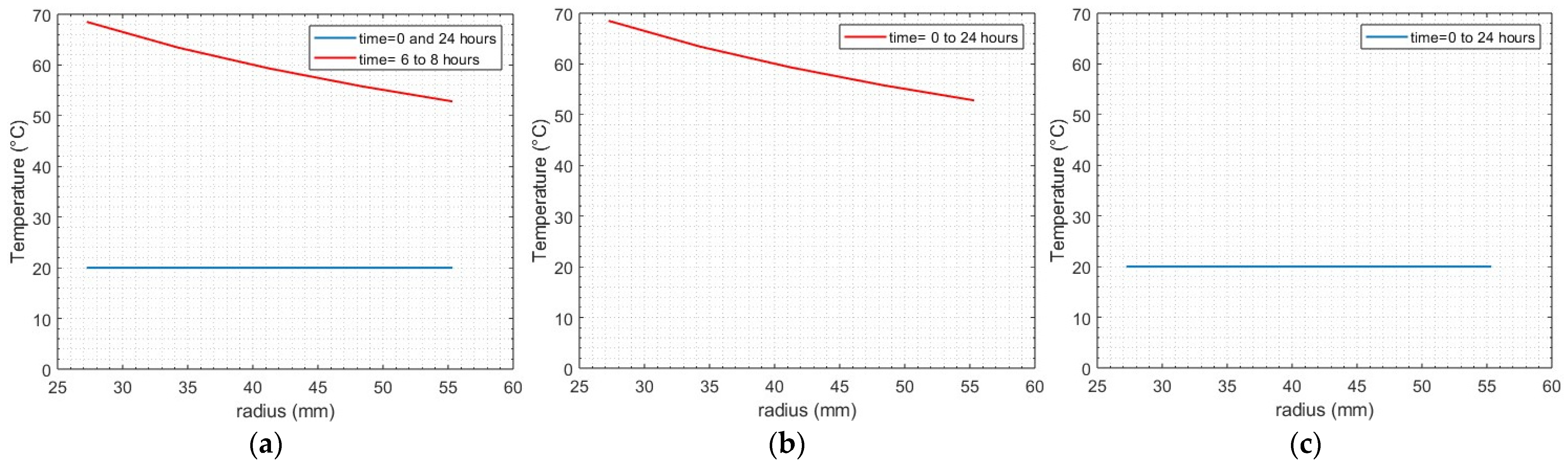
Figure 1 shows the temperature profile within the insulation of a 500-kV DC-XLPE cable during a 24 h load cycle of the LC, HL, and ZL periods, when one sets the conductor temperature T_cond = T_cond,max = 70 °C and temperature drop across cable insulation ΔT = ΔT_max.

Table 1 shows that the sequence of load cycles and the polarity of the applied voltage of the EQT is similar to that of the PQT, while the number of cycles and the test voltage levels are different: 82 cycles for EQT, much less than the 360 cycles for PQT; U_EQ1 = 1.68U₀ for the EQT, which is greater than U_TP1 = 1.45 U₀ for the PQT.

According to [3], the EQT can replace the PQT only in certain circumstances (reported in detail in Cigré TB 852 Section 10.4 [3]), such as when the modifications of the previously qualified cable do not affect the insulation material, the fundamental manufacturing technique, and the electric field level. However, the question arises whether the greater voltage level and the different structure of the EQT compared to the PQT can compensate for the much shorter duration, as well as whether the greater voltage (being farther from the rated voltage U₀) is also representative of the PQT voltage (closer to U₀) of the working conditions of cables in service, with the relevant stresses. In summary, it is important to assess if the EQT is as challenging as the PQT, as well as if it is well representative of the long-term behavior of the cable system down to service stresses. The answers to these questions are very important, especially for cable stakeholders, which have to be well-aware of the differences and consequences of the EQT compared to the PQT. Unfortunately, direct experimental tests on full-size cable systems for answering these questions are practically unfeasible, as illustrated later in this paper.

On the other hand, researchers have developed a procedure for the life and reliability estimation of HVDC cables subjected to qualification load cycles in a series of previous publications [6,7,8,9,10]. The temperature profile and thermal properties of the cable insulation were extensively investigated in [6]. The first development of the reliability model of HVDC cables under load cycles was introduced in [7], while the transient electric field calculations that replaced the approximated analytical electric field calculations were introduced in [9] for PQT load cycles. Different sets of periodic 24 h and 48 h load cycles, i.e., type test load cycles, were applied to the cable in [10].

While in previous works, the authors of this paper studied the life and reliability of various types of HVDC cables under both prequalification and type test conditions [6,7,8,9,10], this paper comes to investigate—for the first time in the literature, as to our best knowledge—the electrothermal life of extruded 500 kV DC-XLPE-insulated cables under EQT load cycles, and to compare the results obtained under EQT conditions with those previously obtained under PQT conditions. Therefore, the results obtained in this paper can help in providing a preliminary answer to the above questions. This goal has been achieved in the present investigation by properly modifying the previously developed procedure for the life and reliability estimation of HVDC cables [6,7,8,9,10]—implemented in the Matlab^TM (R2024b Update 5 (24.2.0.2863752), 64-bit (win64)) environment—to make it applicable to EQT load cycles in addition to PQT and type test load cycles, which are already considered in the former version of the procedure.

This paper is structured as follows. In Section 2, the theoretical background of the procedure for the life and reliability estimation of HVDC cables subjected to qualification load cycles is given, emphasizing the modifications to the previous version of the procedure—and to the relevant Matlab^TM code—implemented in this investigation to make the procedure applicable to EQT load cycles. In Section 3, the case study for the application of the procedure to EQT load cycles and the comparison with PQT load cycles are described. Section 4 illustrates the results obtained, while Section 5 discusses some aspects of the loss-of-life fraction estimation and the validation of the life evaluation algorithm in more detail. In Section 6, a proposal for a modified extension of qualification test (MEQT) is put forward, which is based on the obtained results. Section 7 draws some final conclusions.

2. Theoretical Background

The procedure developed by the authors for the evaluation of the life and reliability of HVDC cables under qualification (i.e., prequalification test and type test [3]) load cycles is illustrated in [7,9,10]. It begins with collecting the data of the cable electrical and thermal properties, the load cycles, and the thermal data of the cable environment. First, the transient temperature during qualification load cycles is calculated inside the insulation thickness. Then, two methods of electric field calculation are chosen for the sake of completeness, i.e., the rigorous numerical computation of the electric field via the solution of Maxwell’s equations and the analytical approximate Eoll’s formula. By knowing the distributions of the transient temperature and electric field within the insulation during qualification load cycles, the fraction of life lost over all qualification load cycles can be estimated at each location within the insulation. Then, the life of the cable under qualification load cycling conditions is estimated, followed by the reliability estimation as a function of time and a final thermal stability check [6]. In [9], the rigorous numerical calculation of the electric field was introduced in the life estimation procedure for 320 kV-HVDC cables subjected to the prequalification test (PQT). Later, in [10], the authors broadened the investigation to include the type test (TT). Subsequently, this procedure has been used to analyze MIND cables as well [11].

The procedure consists of the following stages—or, better, numerical algorithms run in the following sequence:

• 1st stage: algorithm for the computation of the transient temperature in the cable insulation during qualification load cycles;
• 2nd stage: algorithm for the computation of the electric field in the cable insulation during qualification load cycles;
• 3rd stage: algorithm for the evaluation of the electrothermal life of the cable under qualification load cycles;
• 4th stage: algorithm for the evaluation of the reliability of the cable as a function of cycling time;
• 5th stage: algorithm for the final thermal stability check.

As anticipated in the Introduction, in this paper, the above procedure has been improved and broadened to also treat extension of qualification (EQT) load cycles—which are fairly different from TT and PQT load cycles, as shown in Table 1—and the relevant electric field profiles—which, consequently, are fairly different from those obtained during TT and PQT load cycles. The first three algorithms, employed in the case study in Section 3 and Section 4, are explained in detail hereafter, together with the modifications required to adapt them to the EQT, while stages 4 and 5 are skipped here for the sake of brevity (more details on them can be found, e.g., in [6,10]).

By using the improved procedure—and the relevant Matlab^TM code—PQT, TT, and EQT load cycles can be now treated in an exhaustive way with the estimation of transient temperature profiles, transient field profiles, insulation loss-of-life fractions, cable life, and reliability—with the final check on thermal runaway.

2.1. Transient Temperature

The algorithm for the calculation of the transient temperature within the insulation of the cable throughout qualification load cycles (1st step of the procedure) is based on IEC Standard 60853-2 [12]. This algorithm comes from another one previously developed for HVAC cables, which was validated in [13] by comparing the algorithm results with experimental data from [14]. Later on, the algorithm was re-adapted in [7,9,10,11] to HVDC cables. This was quite straightforward, as the transient temperature calculation is simpler for HVDC than for HVAC cables, since the former cables are without skin and proximity effects in the conductor, induce losses in outer metallic layers, and have typically negligible dielectric losses [15]—unless thermal runaway occurs [6].

The temperature profiles in Figure 1 have been calculated using this algorithm.

2.2. Electric Field Distribution

The algorithm for the calculation of the transient electric field within the insulation of the cable throughout qualification load cycles (2nd step of the procedure) performs the computation of the transient electric field profile within the cable insulation by means of the numerical iterative solution of Maxwell’s Equations (1)–(4) [9,10,16]:

$$\nabla ·\left({\epsilon }_0{\epsilon }_r\mathit{E}\right)=\rho$$

(1)

$$\nabla ·\mathit{J}=-\partial \rho /\partial t$$

(2)

$$\mathit{J}=\sigma \mathit{E}$$

(3)

$$\sigma ={\sigma }_0\mathit{exp}\left(a(T-T_0)+b(E-E_0)\right)$$

(4)

where E = electric field vector, J = current density vector, σ = density of free charges, $\sigma$ = electrical conductivity of the insulation, σ₀ = value of $\sigma$ at T₀ = 0 °C and E₀ ≈ 0 kV/mm, $a$ = temperature coefficient of $\sigma$, $b$ = stress coefficient of $\sigma$ [6], ε₀ = permittivity of free space, and ε_r = relative permittivity of the dielectric.

In Equations (1)–(4), $a$ and $b$ coefficients represent the charge conduction characteristics in the cable insulation in the macroscopic conduction model. The coefficient $a$ rules the exponential dependence of conductivity on temperature variation, while the coefficient $b$ governs the exponential dependence of conductivity on the electric field.

The transient electric field calculation algorithm was validated in [9], comparing the algorithm results for a “standard” 450 kV HVDC cable with previous calculations from [17].

The application to the EQT of the procedure for the life and reliability estimation of HVDC cables under qualification load cycles has required adapting the algorithm for transient electric field calculation to EQT load cycles, which feature a different voltage level compared to PQT and TT load cycles, and resetting the step duration in the time domain, the mesh size in the space domain, and the underrelaxation factors in the iterative numerical solution of Maxwell’s equations to ad hoc values. In this way, convergence in the iterative numerical calculation of the electric field has been achieved during the EQT cycles as well.

2.3. Life Evaluation

The algorithm for the calculation of the life of the cable insulation subjected to qualification load cycles (3nd step of the procedure) employs an ad hoc electrothermal life model, called the IPM (Inverse Power Model)-Arrhenius model [2], to assess the lifespan of the HVDC cable under qualification load cycling conditions. Specifically, it estimates the accumulated fraction of life lost by the cable insulation during qualification load cycles (see Table 1 for PQT and EQT), as well as the life of the location of greatest electrothermal stress in the insulation, which determines the cable’s overall life. These estimates rely on Miner’s law of cumulated aging [18], using the equations listed below [7,9,10,11]:

$$L\left(E,T\right)=L_D.[E/E_D{]}^{-(n_D-b_{ET}T″) }{\left[E_D/E_0\right]}^{b_{ET}T″ }{e}^{-BT″}$$

(5)

$${LF}_{cycle}\left(r\right)={\int }_0^{t_d}{\displaystyle \frac{dt}{L[E\left(r,t\right),T(r,t\left)\right]}}={\displaystyle \frac{1}{K_{cycle}\left(r\right)}}$$

(6)

$$L_{cycle}\left(r\right)=t_d\times K_{cycle}\left(r\right)$$

(7)

$$L_{cycle}=min\left\{L_{cycle}\left(r\right),r\in \left[r_i,r_o\right]\right\}$$

(8)

where $L$ is life at DC electric field E and temperature T, T$″=1$/T_D − 1/T (E_D, T_D and L_D being design electric field, temperature, and life of cable insulation, respectively), n_D is the value of life exponent at T_D, B = ∆W⁄K_B, ∆W is the activation energy of the main thermal degradation reaction, K_B = 1.38 × 10⁻²³ J/K is the Boltzmann constant, b_ET is the factor of synergism between the thermal and the electrical stress, LF_cycle(r) is the loss-of-life fraction over all the cycles at a certain radius r within the cable insulation, and K_cycle(r) is the number of cycles to failure at a certain radius r within the cable insulation, with r ranging from the inner insulation radius r_i to the outer insulation radius r_o.

For more details on the algorithm for the evaluation of the life and reliability of HVDC cables under time-varying load cycles—skipped here for brevity—the readers should address [7,9,10,11].

The validation of the algorithm for the calculation of the life of the cable insulation subjected to qualification load cycles (3rd step of the procedure for life and reliability evaluation of HVDC cables under time-varying load cycles) is much more cumbersome than that of the previous two algorithms. It is unfeasible in practice for full-size cables—as illustrated in Section 5—and it is also quite hard for small size test objects as flat specimens or mini cables, because it would require the application of a huge number of transient loads to cover all possible—or at least typical—load cycles encountered on site. To our best knowledge, only constant stress electrothermal life models have been—quite rarely, indeed—validated by comparison with the electrothermal Accelerated Life Test (ALT) [19] results, performed at selected combinations of a constant voltage and temperature. An electrothermal model which was validated in this way is the IPM-Arrhenius model, shown in Equation (5), whose parameters n_D (relevant to the IPM electrical life model), B (relevant to the Arrhenius life model), and b_ET (relevant to the synergism between electrical and thermal stress) were estimated for XLPE and EPR-insulated mini cables tested under various combinations of a constant temperature and constant (in the rms sense) AC voltage at power frequency, as reported, e.g., in [20]. This is the first reason why the IPM-Arrhenius model in Equation (5) was selected for use in this procedure.

The second reason—even sounder in the case of HVDC extruded cables—is that in fact, the IPM-Arrhenius model is the combination of two models, both of which are used in reference International Standards for HVDC extruded cables:

(a)

the IPM electrical life model with L₀ = L_D = 40 years, n₀ = n_D = 10 is the model taken in CIGRÈ TB 852 [3] (the reference Standard for HVDC extruded cables, see above), precisely to establish the voltage level and the duration of TT, PQT, and EQT load cycles (see Appendix A, Clause A.1, of [3]);

(b)

the Arrhenius thermal life model is the reference life model taken in IEC 60216 [21], to provide guidelines for the thermal endurance evaluation of electrical insulating materials—among which extruded insulation for HVDC cables is included.

Therefore, when applied to DC-XLPE cable insulation, the IPM-Arrhenius model is used in the procedure with the following values of parameters: L_D = 40 years, n_D = 10, B = 12,430 K (derived from XLPE mini cable ALT data after [20]), and b_ET = 0 (which can be shown to correspond to the worst case of electrothermal synergism for cable life) [2,8].

For all these reasons, although the validation of the algorithm for the life and reliability evaluation of HVDC cables under time-varying load cycles was not performed in a direct way because it is extremely difficult—or practically unfeasible—the IPM-Arrhenius model used in the procedure can be deemed as a sound, reliable, and accurate tool for electrothermal life estimation.

The application to the EQT of the procedure for the life and reliability estimation of HVDC cables under qualification load cycles has required adapting the algorithm for the evaluation of the electrothermal life of the cable to EQT load cycles, by recasting the calculation of the loss-of-life fractions within load cycling periods to the different durations of the various load cycling periods of the EQT compared to PQT (see Table 1) and TT. This has implied proper modifications, in particular, to relationships (6) and (7), in order to perform the following:

(1)

properly compute the loss-of-life fractions LF_cycle(r) at each cable insulation radius r within the grouped load cycles of the LC, HL, and ZL periods, which have a different duration in the EQT compared to the PQT;

(2)

properly compute the number of cycles to failure K_cycle(r) at each cable insulation radius r.

3. Case Study

The studied cable is a DC extruded cable for use with VSC. It has a rated power of 960 MW in a monopolar scheme under a rated voltage of 500 kV and rated current of 1920 A. The single core conductor is made of copper with a cross-section of 2000 mm². The design temperature of the cable conductor is set to T_cond,max = 70 °C. The conductor is insulated by a 28.1 mm thick DC-XLPE (Cross Linked Polyethylene for DC applications) insulation between two layers of a semiconductive material (usually Polyethylene-based with added carbon black). The design temperature drop across the cable insulation is set to ΔT_max = 15.7 °C. The thickness of the inner semiconductive layer is 2 mm, while the thickness of the outer semiconductive layer is 1 mm. The latter layers are shielded by a 1 mm thick metallic screen. Then, a thermoplastic sheath covers the aforementioned layers with a thickness of 4.5 mm. The design life is considered L_D = 40 years, with a life exponent of n_D = 10. As for the values of life exponent n_D = 10 and design life L_D = 40 y, used in relationship (5), as pointed out at Section 2.3, these values are derived from Appendix A, Clause A.1, of TB 852, where voltages and durations of qualification tests are established, starting from the Inverse Power Model (IPM) with these life exponent and design life values. Since in this study, the EQT according to TB 852 is analyzed, it is important to set these values in the life model (5). In TB 852:2021, the value of life exponent n = 10 is considered as a conservative estimate, although extruded insulations for HVDC cables with values of n greater than 10 have been developed over the years (see e.g., [22,23,24,25,26]).

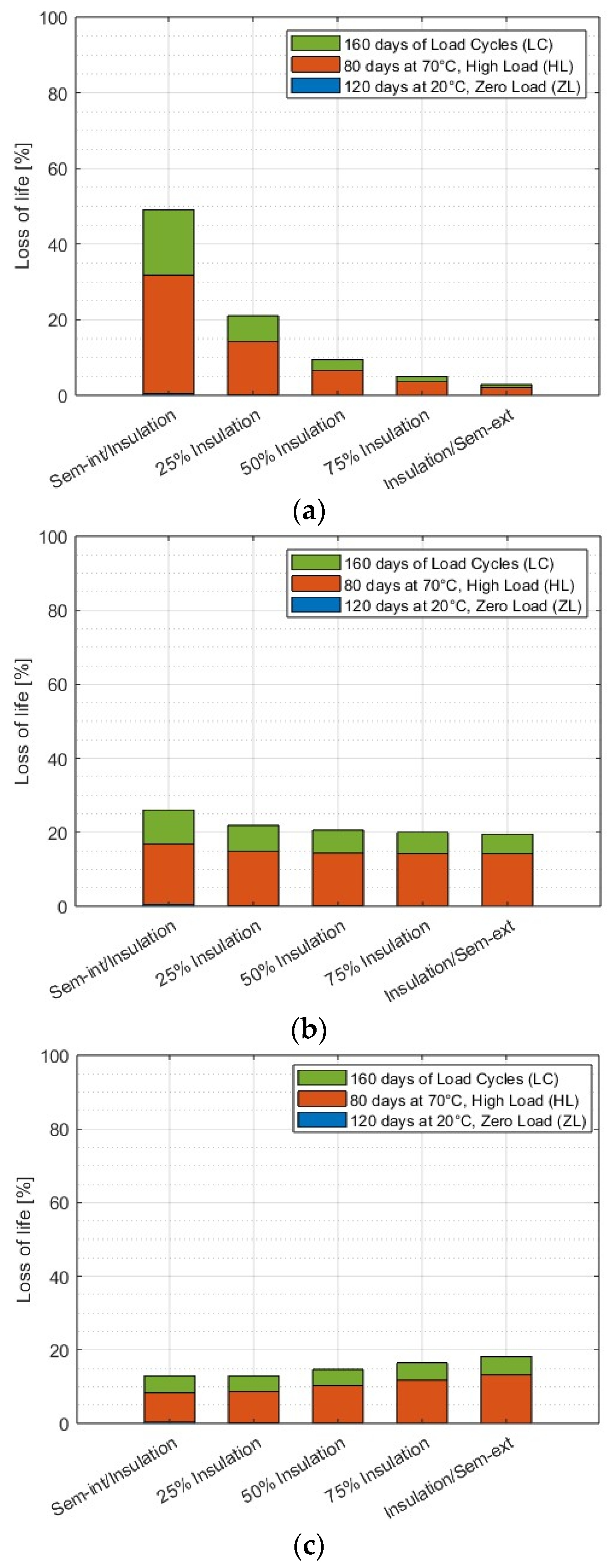
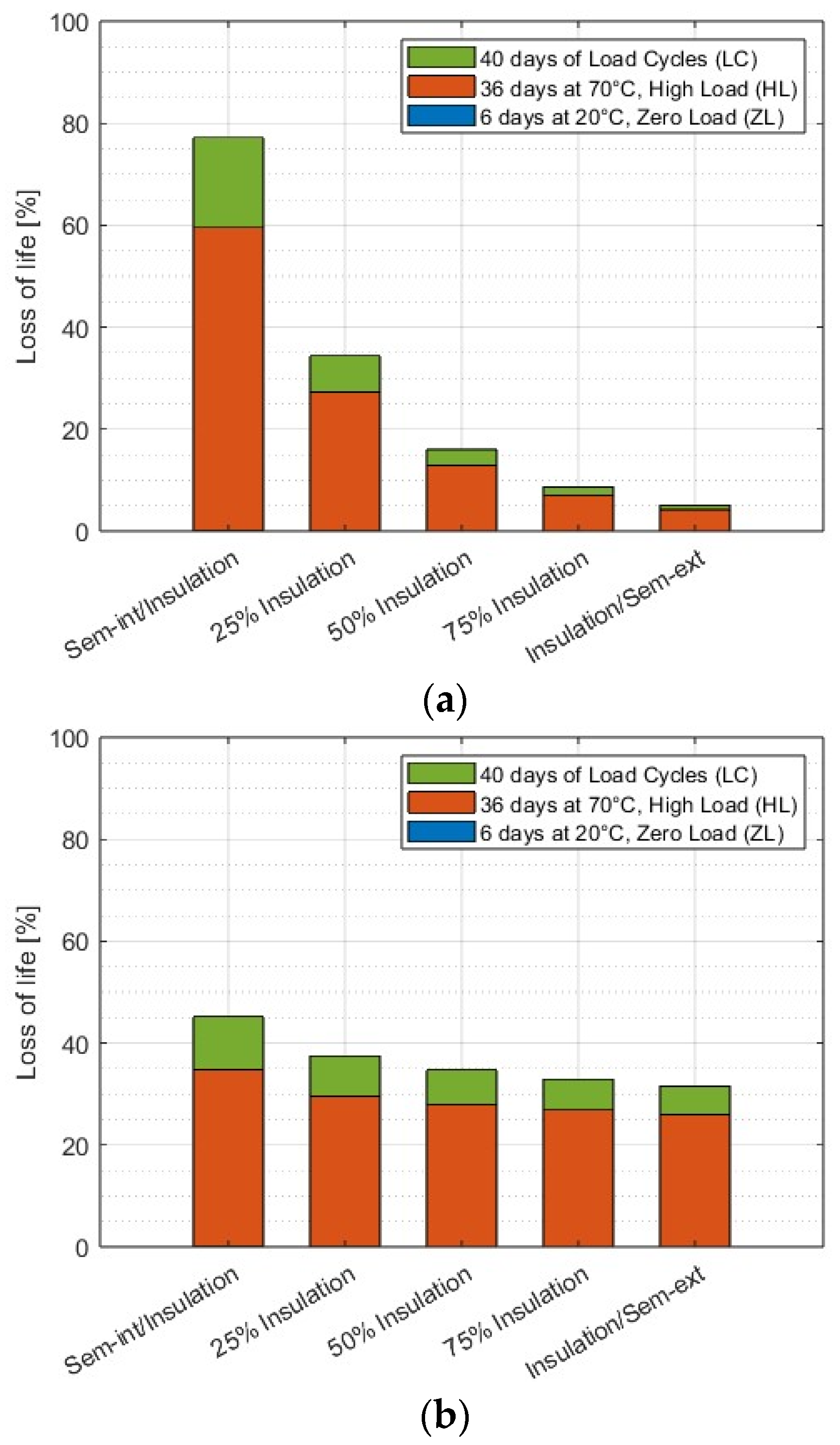
The cable undergoes PQT load cycles, i.e., 160 “24-h” LC, 80 HL, and 120 ZL load cycles; then (in another simulation run), it undergoes EQT load cycles, i.e., 40 “24-h” LC, 36 HL, and 6 ZL load cycles according to TB 852 (see Table 1) [3]. The calculations are carried out for three different sets of values of $a, b$ coefficients (see

Table 2. Sets of $a, b$ coefficients of electrical conductivity.

	$\mathit{a}$ [1/°C]	$\mathit{b}$ [mm/kV]
Low set (aL, bL)	0.042	0.032
Medium set (aM, bM)	0.084	0.0645
High set (aH, bH)	0.101	0.0775

), in order to scan the various conductivity behaviors of different insulation compounds. Further attention will be given to the medium values that represent DC-XLPE insulation in the literature [27,28].

4. Results

4.1. Electric Field Distribution

The transient electric field profile in the cable insulation is computed according to Equations (1)–(4) for the three sets of conductivity coefficients (as in Table 2) under PQT and EQT conditions (applied DC voltage U_EQT1 = 1.68U₀). Figure 2 displays the electric field profile within the case study cable insulation in different situations. Figure 2a shows the steady-state resistive (or ohmic) DC field profiles during the PQT (test voltage U_TP1 = 1.45U₀, solid curves) and EQT (test voltage U_EQ1 = 1.68U₀, dashed curves), for the case study cable in hot conditions, i.e., T_cond = T_cond,max = 70 °C and ΔT = ΔT_max = 15.7 °C (red curves), and in cold conditions, i.e., T_cond = 20 °C and ΔT = 0 (blue curves), obtained for medium values of $a, b$ coefficients of electrical conductivity. The hot cable profile and the cold cable profile are those to which the transient temperature profiles within the insulation tend, respectively, during the heating part and the cooling part of LC cycles of the PQT and EQT (see Table 1); the hot cable profile and the cold cable profile are reached, respectively, during the HL and ZL periods of the PQT and EQT, as the HL and ZL periods last much longer than the typical dielectric time constant of the cable insulation (see Appendix A, clause A4, of [3]). Figure 2a highlights that, as the cable is heated—inner insulation tends to become warmer than outer insulation—the ohmic electric field tends to drop at the inner insulation and to rise at the outer insulation. Depending on the values of a, b, the so-called field inversion may take place, where the electric field at the outer insulation becomes greater than that at the inner insulation. This does not happen for low values of a, b, while it does happen for medium values (as in Figure 2a) and high values of a, b.

Figure 2b shows the field variation from the initial instant (black curve) towards the ohmic electric field during the HL period in the LC (blue, green, and red curves in the case of low, medium, and high values of $a, b$ coefficients of electrical conductivity, respectively). In the case of a_L, b_L, an electric field stabilization takes place where the electric field in the inner insulation is almost similar to that at the outer insulation. While in the case of a_M, b_M, and a_H, b_H, the electric field is inverted.

4.2. Fraction of Life Lost

The fraction of life lost at every single point of case study cable insulation throughout the load cycles is calculated according to (5) and (6) as a summation of the fraction of life lost at that point in each elementary time interval. Figure 3 presents the total percent loss of life during load cycles (LCs), high load (HL), and zero load (ZL) periods of the PQT at five equally spaced points inside the insulation of the case study cable, including the inner insulation surface and the outer insulation surface. Indeed, according to previous investigations [6,7,10,11,16], the most stressed point that features the greatest loss of life is typically located either on the inner insulation surface or at the outer insulation surface, depending on the loading and on the relevant field distribution (see Figure 2). The selection of five equally spaced points comes mainly from the macroscopic conduction model used in this paper, where the charge is smoothly distributed across the insulation thickness, as broadly discussed in [17,29,30]. The life under load cycles is estimated at each point, depending on the time-varying electric field and temperature at this point throughout the load cycles, according to Equations (5)–(7). It is clear from the equations—in particular from the IPM Arrhenius life model under constant electrothermal stress—that the increase in the temperature and/or the electric field leads to a shorter life and more loss of life at this point. By estimating the life at different points inside the insulation thickness, the comprehensive life of the cable is assumed to be equal to that of the point with the shortest life across the insulation thickness (see Equation (8)).

From Figure 3, it can be noticed that 80-day HL cycles have the greatest electrothermal stress and loss of life, followed by the LC period, which lasts for 160 days. The fraction of life lost during ZL cycles is barely noticeable.

In Figure 3, the loss of life varies across the insulation due to the transient thermal and electrical stresses. The most stressed point within the insulation is also related to the values of electrical conductivity coefficients of the dielectric, namely, $a,b$ (see (4) and Table 2), which define the conductivity dependence, respectively, on the temperature and field. Figure 3a shows the loss of life for low values of $a,b$: here, the inner insulation surface is the most stressed location within the insulation affected by the stabilized electric field distribution, and it has a greater temperature compared to the one at the outer insulation surface. Figure 3b shows a more uniform loss-of-life distribution over the insulation points for medium values of $a,b$. The inner insulation is more stressed compared to the outer insulation, although the electric field inversion begins to occur (Figure 2). The higher temperature of the inner insulation compared to the outer insulation in the 500 kV cable can justify this result (see Figure 1). The total loss of life becomes greater at the outer insulation for high values of $a,b$, where the electric field is more inverted and becomes able to overcome the temperature (as in Figure 3c).

Figure 4 illustrates the total percent of the loss of life within the insulation thickness of the case study cable subjected to EQT conditions in the case of low, medium, and high values of the conductivity coefficients $a,b$. In Figure 4, the pattern of the loss of life during the EQT is qualitatively similar to that of the PQT in Figure 3. This qualitative similarity of the lifetime loss in the 82 days of the EQT compared to the much longer 360 days of the PQT, is due of course to the higher test voltage of the EQT (1.68U₀) compared to that of the PQT (1.45U₀), which implies overall greater values of the applied electric field inside the insulation. However, from a quantitative viewpoint, the loss-of-life values are much greater in the EQT compared to the PQT. For example, consider the most stressed point (77%, 45%, and 28%) in the EQT compared to that (49%, 26%, and 18%) in the PQT for low, medium, and high $a,b$, respectively. This can be justified by the greater thermal stress applied to the cable during the EQT with respect to the PQT, as HL cycles are much more than ZL cycles in the EQT compared to the PQT (see Table 1). This can be confirmed by comparing the LC bars (green) and HL bars (red) in Figure 3 (=PQT) and Figure 4 (=EQT), where the loss of life during LC periods are similar in the PQT and EQT. While the loss of life during the HL period of the EQT is approximately double that during the HL period of the PQT, the patterns are still similar.

4.3. Life Estimation

Figure 5 displays the cable life at five points distributed across the insulation, starting from the inner insulation surface (point 1) and ending at the outer insulation surface (point 5), for low, medium, and high values of conductivity coefficients $a, b$, when the cable is subjected to the PQT (in Figure 5a) and EQT (in Figure 5b). From these figures, it is readily seen that, according to the life estimation procedure, the cable passes with a fairly broad margin both the PQT and the EQT, withstanding the applied electrothermal stress satisfactorily. Indeed, all life points have greater values than the duration of the PQT (360 days ≈ 1 year in Figure 5a) and EQT (82 days in Figure 5b), which is illustrated as a black dashed line. In both the PQT and EQT, (Figure 5a and Figure 5b, respectively), the most stressed location across the insulation is the inner insulation for a_L, b_L and a_M, b_M, while it shifts towards the outer insulation for a_H, b_H. For a_M, b_M, the field inversion (see Figure 2) does not lead to an inversion of the life pattern because thermal stress overwhelms the electrical stress in both the PQT and EQT. In the case of a_H, b_H, the inverted electrical stress starts to overwhelm the thermal stress. In the case of the PQT (Figure 5a), the cable life ranges between 734 days ≈ 2 years, 1378 days ≈ 4 years, and 2774 days ≈ 5.5 years for low, medium, and high values of a, b, respectively. In the case of the EQT (Figure 5b), the life of cable ranges between 106, 181, and 288 days for low, medium, and high values of $a,b$, respectively.

In addition to the graphical results shown in Figure 5,

Table 3. Estimated life (days) at the above 5 points under PQT conditions for low, medium, and high sets of conductivity coefficients.

Point	aL, bL	aM, bM	aH, bH
1	734	1378	2774
2	1709	1644	2773
3	3805	1748	2448
4	7198	1801	2183
5	12,571	1840	1982

and

Table 4. Estimated life (days) at the above 5 points under EQT conditions for low, medium, and high sets of conductivity coefficients.

Point	aL, bL	aM, bM	aH, bH
1	106	181	354
2	238	218	362
3	512	236	331
4	943	249	306
5	1599	260	288

report the estimated cable life in days at the above five points under PQT and EQT conditions, respectively, for different sets of conductivity coefficients (a, b); to further facilitate the comparison with the test durations,

Table 5. Estimated cable life in p.u. with respect to PQT duration (360 days), at five radial positions and for different conductivity coefficient sets.

Point	aL, bL	aM, bM	aH, bH
1	2.04	3.83	7.71
2	4.75	4.57	7.70
3	10.57	4.86	6.80
4	19.99	5.00	6.06
5	34.92	5.11	5.51

and

Table 6. Estimated cable life in p.u. with respect to EQT duration (82 days), at five radial positions and for different conductivity coefficient sets.

Point	aL, bL	aM, bM	aH, bH
1	1.29	2.21	4.32
2	2.9	2.66	4.41
3	6.24	2.88	4.04
4	11.5	3.04	3.73
5	19.5	3.17	3.51

present the same life estimations expressed in per unit (p.u.) values with respect to the PQT duration (360 days) and EQT duration (82 days), respectively.

These tables confirm the trends observed in Figure 5 and highlight the influence of the conductivity parameters on the stress distribution and life expectancy across the insulation thickness.

5. Discussion

These results deserve more analysis and discussion, especially those relevant to loss-of-life fraction and life estimation.

In particular, to confirm the thermal effect of the fractions of life lost in the HL period with respect to those in the LC period in both the PQT and EQT (the fraction of life lost during ZL cycles is practically irrelevant, as hinted at above), the fractions of life lost in the HL and in the LC period have also been estimated with a simplified version of the IPM-Arrhenius electrothermal life model (5). In such a simplified version of the IPM-Arrhenius model, the IPM electrical life model and the electrothermal synergism factor are replaced with the life model used in [3], Appendix A, clause A.1, to determine the test voltage U_T from the system voltage U₀, design life L_D, and test duration L_T (in clause A.1 of [3], U_T = V_dc, U₀ = V₀, L_D = t₀ = 40 years, L_T = t₁), namely:

$$L_D.[E/E_D{]}^{-(n_D-b_{ET}T″) }{\left[{\displaystyle \frac{E_D}{E_0}}\right]}^{b_{ET}T″ } \approx L_T=L\left(U_T\right)=L_D{\left(U_T/U_0\right)}^{-n_D}$$

(9)

where, consistently with [3], Appendix A, clause A.1, n_D = 10, as in Equation (5). Of course, this model yields L_PQT = 360 days when U_T = U_TP1 = 1.45U₀ and L_EQT = 82 days when U_T = U_EQ1 = 1.68U₀.

By inserting (9) in (5) in place of the IPM and of the electrothermal synergism factor, only the Arrhenius thermal life model is left active, thereby excluding the electric field effect on the loss of life, as follows.

$$L\left(E(r,t),T(r,t)\right)\approx L\left(U_T,T(r,t)\right)=L_T{ e}^{-B \left({\displaystyle \frac{1}{T_D}}-{\displaystyle \frac{1}{T(r,t)}}\right)}$$

(10)

where T(r,t) is the transient temperature at radius r within cable insulation and at time t during the load cycles, as in Figure 1. B = 12,430 (K) for DC-XLPE comes from the results after [20] for XLPE-insulated mini cables.

Introducing this simplified version of Equation (5) in the algorithm for life evaluation (3rd step of the procedure described in Section 2, see Section 2.3), the values of the ratio

$${\displaystyle \frac{{LF}_{HL}}{{LF}_{LC}}}={\displaystyle \frac{loss of life throughout all load cycles of the whole HL period }{loss of life throughout all load cycles of the whole LC period}}$$

(11)

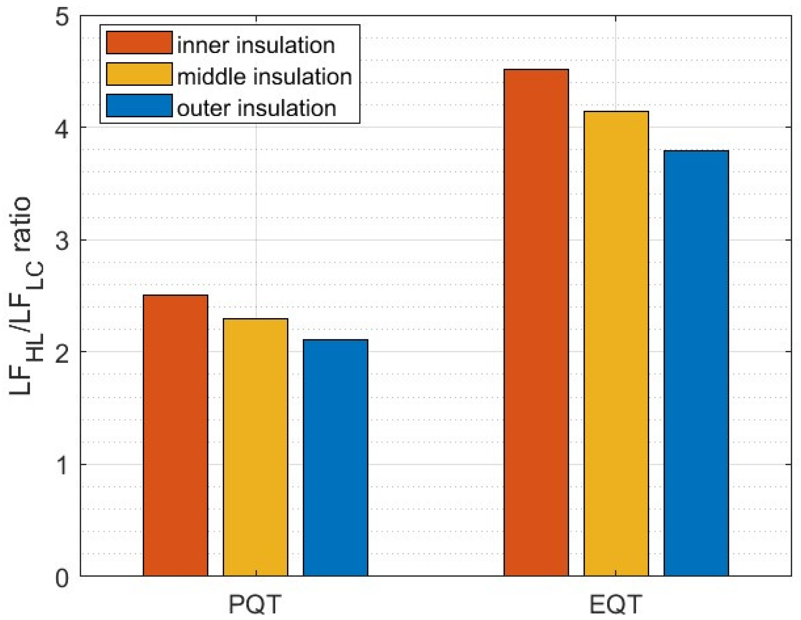
have been calculated at the inner insulation surface, 50% of insulation thickness (=middle insulation), and outer insulation surface for the PQT and EQT. Figure 6 shows the bar plot of the ratio LF_HL/LF_LC for the PQT (left part of Figure 6) and the EQT (right part of Figure 6). These same values are listed in

Table 7. LF_HL/LF_LC ratio using the Arrhenius simplified calculations (see Equations (9) and (10)) and the electrothermal life estimation reported for PQT (in Figure 3) and EQT (in Figure 4) at inner, medium, and outer insulation for the three different conductivity coefficient sets.

Test	Method	a, b Set	Inner Insulation	Middle Insulation	Outer Insulation
PQT	Arrhenius simplified	N/A	2.5	2.3	2.1
	E-T rigorous (Figure 3)	aH, bH	1.8	2.3	2.8
		aM, bM	1.8	2.3	2.6
		aH, bH	1.7	2.3	2.6
EQT	Arrhenius simplified	N/A	4.5	4.1	3.8
	E-T rigorous (Figure 4)	aL, bL	3.4	4.3	4.8
		aM, bM	3.3	4.1	4.6
		aH, bH	3.2	4.1	4.7

for a more accurate comparison with the values of the ratio LF_HL/LF_LC obtained when using the rigorous IPM-Arrhenius electrothermal model in Equation (5) of the procedure with the three sets of a, b coefficients for the PQT and the EQT; note that these latter values—referred as “E-T” rigorous values in Table 7—can be deduced from Figure 3a–c and Figure 4a–c, respectively, for the PQT and EQT with a_L, b_L, a_M, b_M, and a_H, b_H.

The values of the ratio LF_HL/LF_LC reported in Figure 6 and Table 7 are all greater than 1: this clearly emphasizes that the loss of life during the whole HL period is greater than that during the whole LC period (overall ≈2 times and ≈4.5 times greater in PQT and EQT, respectively). It also emphasizes that the loss-of-life ratio is greater in the EQT compared to the PQT, due to the longer duration of the HL period in the EQT compared to the duration of the HL period in the PQT, as hinted at above. Hence, the approximate results obtained with the Arrhenius model agree overall with the findings and the discussion of the algorithm used in this paper by applying the electrothermal life model.

In addition, let us note that the results in Table 7 can be explained more in detail as follows.

• When the Arrhenius simplified approach is used, only temperature is active in degrading the cable insulation; since the inner insulation always has the highest temperature—and this happens steadily during the whole HL—inner insulation has the greatest loss of life and the ratio LF_HL/LF_LC is the greatest at the inner insulation. On the contrary, moving from the inner to outer insulation, the situation is the opposite. Indeed, the outer insulation has the lowest temperature—and this happens steadily during the whole HL—hence, it has the lowest loss of life, and the ratio LF_HL/LF_LC is the lowest at outer inner insulation.
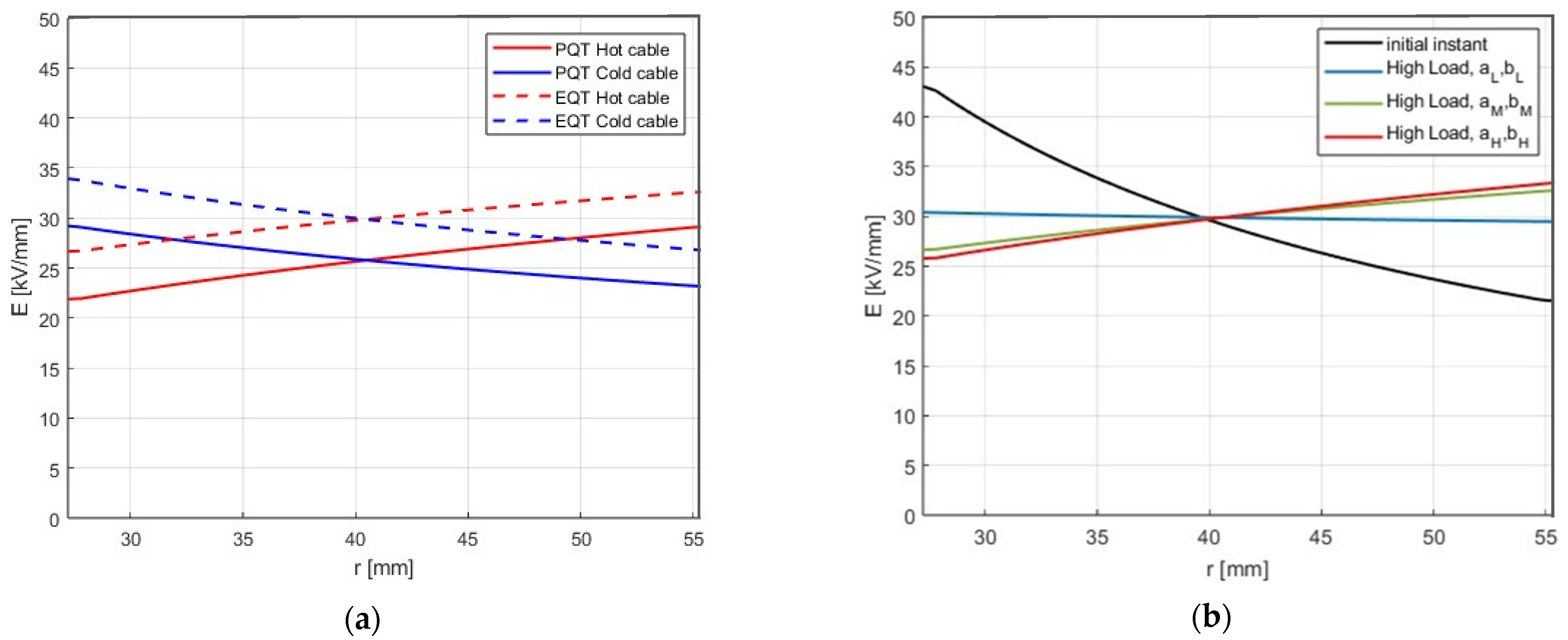
• When the rigorous electrothermal approach is used, the inner insulation during the HL period has a lower field than at room temperature due to the higher temperature (remember that the field at inner insulation drops as temperature increases, see Figure 2a), and this reduces the field-induced loss of life during the HL period (although the ratio remains >1); conversely, the outer insulation during the HL period has a higher field than at room temperature due to the higher temperature (remember that the field at the outer insulation rises as temperature increases, see Figure 2a), and this raises the field at the outer insulation and increases the field-induced loss of life during the LC. Hence, the ratio LF_HL/LF_LC is the lowest at the inner insulation, increases at the middle insulation, and is the highest at the outer insulation when the rigorous electrothermal approach is used.

Let us emphasize that—as hinted at in Section 2—the transient thermal calculations (1st step of the procedure) and the transient electric field calculations (2nd step of the procedure) have been validated with an independent validation (namely, comparison with experimental case for the 1st step, see Section 2.1, and a software developed by other authors for the 2nd step, see Section 2.2), so no more doubts should arise about the precision of the code’s outputs for field and temperature. On the contrary, the direct experimental validation of the life estimation algorithm (3rd step of the procedure), although relying on a sound and validated constant stress electrothermal life model—the IPM-Arrhenius model—and on the good old Miner’s law of cumulated aging, is practically unfeasible for full-size cable systems (see Section 2.2). Let us explain here in more detail why; this is essentially for two reasons.

(1)

The detailed results of the PQT and EQT—with the description of possible failures and failure times—are kept confidential by the involved parties, namely manufacturers and utilities.

(2)

The validation of (life lost and) life estimates for full-size cable systems would require finding a manufacturer available to arrange, in a huge and dedicated lab, a suitable number of cable loops for the PQT, as well as for the EQT (say, three as a minimum, from five to ten for a better statistical processing required for accuracy estimation), apply PQT load cycles, as well as EQT load cycles, and wait for a time long enough to cause the breakdown of all loops for the sake of good statistical processing; eventually, results would have to be processed and estimates of the kind provided by our procedure would have to be derived. Our computations (see Table 5) show that for the PQT, the average failure time might range from two to five times the duration of the test, i.e., from 2 to 5 years, but also long-lasting outliers have to be accounted for: the last breakdown might take even more than two to three times the average, i.e., more than 10–15 years for the PQT! The same procedure should be repeated for the EQT: this would take something less than one-quarter of the time spent for the PQT (see Table 6), but this is still a few years! Of course, this experimental procedure is unfeasible—and even if it were feasible, no manufacturer would disclose these results.

This is precisely the reason why this simulation procedure and the relevant algorithms have been developed, first for the TT and PQT, and here for the EQT. And since the third algorithm is the hardest to verify, it can be deemed as very satisfactory if the life estimates obtained are in line with the experimental evidence of qualification tests—as their results are more or less fuzzily disclosed by manufacturers and utilities in a generic way—namely, well-designed, manufactured, and installed cables do pass qualification tests without problems—and going down to service stresses, CIGRE TB 815:2015 [31] confirms this satisfactory long-term behavior obtained in the PQT with the extremely rare failures reported for HVDC cables in service until 2015, all qualified according to TB 219:2003 [4] and TB 496:2012 [5], thus in the absence of the EQT option. This outcome is perfectly in line with the results in Table 3 and Table 5 for the PQT, as well as with those in Table 4 and Table 6 for the EQT. In particular, Table 5 and Table 6 show that the time to failure forecasts obtained with the procedure illustrated here are always longer than the duration of the PQT and EQT, respectively. This is indirect evidence that the procedure is satisfactory—although its accuracy for a life estimate cannot be evaluated. The alternative would be simply doing nothing, i.e., refraining from estimating life and reliability simply because the accuracy of the procedure cannot be directly evaluated. As engineers, the authors aim at providing cable stakeholders with tools that help solve problems: this is the reason why in the authors’ opinion, it is preferable to provide an uncertain estimate—in line, or not against, the experimental evidence—than doing nothing. In the end, utilities companies always ask power cable engineers the following: “how long will this cable last in certain conditions?”

For this reason, in our opinion, the best comparison to be made for validating these results is the comparison with the PQT and EQT test durations (see Table 5 and Table 6), as this provides an estimation about whether the cable will withstand the test or not. Table 5 and Table 6 reveal that the most stressed point always has a life greater than the duration of the PQT and the EQT, respectively, for all the conductivity coefficient sets. This indicates that the case study cable will pass both the EQT and the PQT load cycles. Hence, the results of the analysis carried out in this paper are in fair agreement with the common general evidence that well-designed, manufactured, and installed HVDC extruded cable loops do pass the PQT and EQT with broad margin. This is certainly an indirect, but important experimental validation of the results obtained. However, the p.u. values of life in Table 5 (namely those for the PQT) are greater than the homologous values in Table 6 (namely those for the EQT). This indicates that EQT conditions are overall more stressful than PQT conditions—at least for this case study cable, but similar results are obtained for other cable types, omitted for brevity here.

6. Proposal for a Modified Extension of Qualification Test Procedure

It should be noted that EQT load cycles are performed at a voltage which is much greater than the rated voltage of the cable system U₀ compared to the PQT, and conversely, the duration of the EQT load cycles is much shorter than the design life of the cable system, L_D. Hence, if it is true that the EQT shortens the testing times and emphasizes the role of high load conditions, its capability to really assess the long-term behavior of the cable system in testing conditions representative of service conditions is poorer than that of the PQT.

Therefore, as a response to the findings and results revealed in this paper, the authors propose two novel modified test procedures for the extension of qualification test, namely, modified extension of qualification test 1 (MEQT1) and modified extension of qualification test 2 (MEQT2). The main aim of this technical proposal is to make a compromise between the beneficial need to speed up the long-term tests (in certain conditions), as in the EQT, while keeping the results predictive of real-world performance, as in the long-term load cycles of the PQT.

The details of the two proposals, MEQT1 and MEQT2, in terms of applied constant DC voltage, overall duration, and duration of the load cycling periods, are reported and compared with the PQT and EQT in

Table 8. Comparison of load cycling periods durations in the PQT, EQT, and in two new proposals for a modified EQT: MEQT1 and MEQT2.

Cycles (Days)	PQT	EQT	Duration Ratio (PQT/EQT)	MEQT1	Duration Ratio (MEQT1/PQT)	MEQT2	Duration Ratio (EQT/MEQT2)
LC	40	10	0.25	20	0.5	22	0.45
LC	40	10	0.25	20	0.5	22	0.45
HL	40	18	0.45	20	0.5	39	0.46
HL	40	18	0.45	20	0.5	39	0.46
ZL	120	6	0.05	60	0.5	14	0.43
LC	40	10	0.25	20	0.5	22	0.45
LC	40	10	0.25	20	0.5	22	0.45
Total	360	82	0.23	180	0.5	180	0.45
UT/U0 (p.u.)	1.45	1.68	-	1.55	-	1.55	-

. As Table 8 shows, the two proposals MEQT1 and MEQT2 are based on extending the total EQT duration to 180 days instead of 82 days and reducing the test voltage from U_EQT1 = 1.68U₀ to U_MEQT = 1.55U₀: this latter value has been determined following the same approach as for U_TP1 and U_EQT1 in Appendix A, Clause A.1 of TB 852 [3], namely, using the IPM of Equation (9). The difference between MEQT1 and MEQT2 is the value of the ratio between the duration of the three cycling periods LC, HL, and ZL, and the overall duration of the test, as follows:

(A)

the 1st proposal, i.e., MEQT1, keeps the same ratio between the duration of LC, HL, and ZL periods and the overall test duration as in the PQT;

(B)

the 2nd proposal, i.e., MEQT2, practically keeps the same ratio between the duration of LC, HL, and ZL periods and the overall test duration as in the EQT.

Since the difference is the ratio between the duration of the three cycling periods LC, HL, and ZL and the overall duration of the test, selecting MEQT1 means following the structure of the PQT and giving all three periods a fairly similar weight compared to the overall duration of the test, while selecting MEQT2 means following the structure of the EQT and giving much more emphasis to the high load period and its enhanced thermal stress, as one might have easily guessed qualitatively, but this investigation has highlighted more accurately in a quantitative way.

Of course, these are just preliminary proposals that should be broadly discussed in the scientific community, also based on the experience gathered in the PQT and EQT.

7. Conclusions

In this paper, the authors investigated the electrothermal life of DC-XLPE-insulated cables that underwent the prequalification test (PQT) and extension of qualification test (EQT) conditions according CIGRÉ Technical Brochure 852. First, the transient temperature across the insulation was computed throughout the PQT and EQT load cycles. Then, the transient electric field profile was computed, considering three sets—i.e., low, medium, and high—of coefficients of electrical conductivity. The calculations are closed with the evaluation of the fractions of life lost throughout the cycles and of the life of DC-XLPE insulation.

The results show similar patterns of fractions of life lost and life across the insulation in both the PQT and EQT, where the insulation experiences the greatest stress at its inner surface for low and medium set of conductivity coefficients, and at its outer surface for high set conductivity coefficients. According to the electrothermal life model, the studied cable is expected to pass both the PQT and EQT and to withstand the electrothermal stresses applied during both tests. Hence, the results of the analysis carried out in this paper—in agreement with other studies relevant to similar cables, omitted here for the sake of brevity—are in fair agreement with the common general evidence that well-designed, manufactured, and installed HVDC extruded cable loops do pass the PQT and EQT with broad margin. This is certainly an indirect but important experimental validation of the results obtained.

The results show that the electrothermal loss of life during the EQT is double that during the PQT compared to the duration of each test (i.e., 360 days and 82 days, respectively). The dominance of high load cycles in the EQT compared to only a few zero load cycles might be the justification (the HL percentage of the total test duration is 44% in EQT compared to only 22% in PQT).

However, it should be noted that EQT load cycles are performed at a voltage which is much greater than the rated voltage of the cable system U₀ compared to the PQT, and conversely, the duration of the EQT load cycles is much shorter than the design life of the cable system, L_D. Hence, if it is true that the EQT shortens the testing times, its capability to really assess the long-term behavior of the cable system in testing conditions representative of service conditions is poorer than that of the PQT. For this reason—notwithstanding the fact that the EQT seems quite challenging in terms of loss-of-life fraction and estimated life—the PQT is recommended as an optimal compromise between the contrasting needs of, on the one hand, reducing testing time and, on the other hand, reproducing cable system stresses in service as closely as possible.

As an alternative, as well as a response to the findings of this paper, the authors propose two novel modified test procedures for the extension of qualification test, namely, modified extension of qualification test 1 (MEQT1) and modified extension of qualification test 2 (MEQT2), their difference being the value of the ratio between the duration of the three cycling periods LC, HL, and ZL and the overall duration of the test; selecting MEQT1 means following the structure of the PQT and giving all three periods a fairly similar weight compared to the overall duration of the test, while selecting MEQT2 means following the structure of the EQT and giving much more emphasis to the high load period and its enhanced thermal stress, as this investigation has highlighted in a quantitative way. The main aim of this technical proposal is to make a compromise between the beneficial need to speed up the long-term tests (in certain conditions) as in the EQT, while keeping the results predictive of real-world performance as in the long-term load cycles of the PQT. Of course, these preliminary proposals should be broadly discussed in the scientific community, also based on the experience gathered in the PQT and EQT.