Energy Efficiency and Environmental Technologies in Carbon Emissions Reduction Strategies for a Sustainable Future: Estimation Through Simultaneous Equation Systems

Abstract

Energy is at the center of economic growth and environmental sustainability. Increasing energy efficiency and turning to environmentally friendly technologies are indispensable elements not only in reducing carbon emissions but also in supporting the transition to a green future. This study aims to deeply examine the simultaneous dynamic interactions between energy, environmental technologies, and economic growth by focusing on the environment and analyzing the transformative effects of these factors on environmental sustainability from a broad perspective. The models were estimated via simultaneous equation systems with two-stage and three-stage least squares methods with monthly data for Organization for Economic Cooperation and Development (OECD) countries between 1990 and 2021. As a result of the analyses, the estimation results of the two methods generally support each other. Notably, economic growth causes carbon emissions, and when tax revenues on energy are added to the model, the negative effect of economic growth on carbon emissions turns positive. Another significant result shows that energy efficiency does not reduce carbon emissions. Even an increase in energy efficiency causes an increase in carbon emissions, and the rebound effect is valid. Population and energy density do not have a negative impact on carbon emissions.

1. Introduction

Energy plays a vital role in every aspect of daily life, from electricity to heating and communication to production, at the center of life. Energy is the fundamental building block of modern societies and the key to economic growth, technological advancement, and social well-being. With the increasing population and industrialization, the energy demand is rapidly increasing. However, the increasing demand for energy and the reliance on fossil fuels to meet this demand have led to serious global environmental problems. Carbon dioxide emissions are one of the leading problems and the most important factor causing climate change.

In this context, transitioning to sustainable energy sources and increasing energy efficiency are crucial. In neoclassical growth theory, energy efficiency, as a part of technological development, is traditionally seen as a driving force of economic growth [1]. When energy efficiency increases, it provides both economic and environmental benefits. Less energy consumption reduces energy costs and increases the competitiveness of businesses. Moreover, lower carbon emissions play a critical role in combating climate change and supporting environmental sustainability.

The relationship between economic growth and carbon emissions is complex and multidimensional. An increase in economic activities increases energy consumption, directly leading to increased carbon emissions. However, this relationship is not always linear. Factors such as technological advances, energy efficiency, and the transition to renewable energy sources can affect the direction and degree of the relationship between economic growth and carbon emissions. Innovative technologies and policies that increase energy efficiency can reduce carbon emissions and mitigate the environmental impacts of economic growth. For example, using energy-efficient appliances and green energy sources can provide lower carbon emissions at the same level of economic growth.

In recent years, significant developments have been made in the field of environmental technologies, especially in areas such as carbon capture and storage (CCS), smart grid systems, and green hydrogen production. These technologies aim to support decarbonization in the industry while maintaining economic efficiency.

Developments in environmental technologies have played an important role in strategies for reducing carbon emissions. In addition to supporting decarbonization, these technologies also contribute to protecting the environment and increasing energy efficiency. Environmental technologies, Carbon Capture and Storage (CCS) systems, direct air capture (DAC) technologies, and biochar applications are methods that aim to directly reduce greenhouse gas concentrations in the atmosphere. New-generation sorbent materials, especially those used in DAC systems, increase the economic viability of the technologies by providing high carbon capture capacity with lower energy [2]. In addition, waste-to-energy systems integrated with circular economy principles facilitate waste management and expand the potential of renewable energy production [3]. Sweden has one of the most advanced systems in the world in terms of waste management and energy recovery. A high rate of domestic waste is recovered and converted into energy. Thanks to “Waste-to-Energy (WTE)” facilities, both energy is produced, and regular landfills are minimized. Sweden operates these facilities by importing waste from other countries and reducing carbon emissions. In addition to Sweden, many other countries are experiencing significant development. Germany stands out in environmental technologies with smart energy grids developed within the scope of “Energiewende” and systems that enable the integrated operation of renewable energy technologies.

Japan, a pioneer country that actively uses carbon capture and storage (CCS) technologies, has its first full-chain CCS project, the Tomakomai Project, which captures and stores CO₂ from a coastal oil refinery on Hokkaido Island, Japan. After a certain pressure is applied to the captured carbon dioxide, it is delivered to the well, and the carbon dioxide is sent to the geological layers under the seabed through the pipe [4]. Japan reduces its high CO₂ emissions with underground carbon storage facilities, such as the Tomakomai project, and thus, shows that it will play an important role in reaching net-zero emissions worldwide.

Concrete and cement, which are common binding materials of concrete, have a significant share of carbon emissions. Cement constitutes only 10–15% of the mass of the material, whereas it constitutes 80–90% of carbon emissions. Cement production is responsible for approximately one-fourth of all industrial carbon dioxide emissions and approximately 7-8% of global CO₂ emissions, causing 2.5 billion tons of carbon dioxide emissions per year [5]. Decarbonization of the necessary materials used in buildings, roads, bridges, and more is an important part of achieving the net-zero emission target. Therefore, it is inevitable that these materials, which are not easy to substitute, will also be used in environmental technologies.

In the face of traditional concrete production that causes such high carbon emissions, carbon-negative concrete developed with the contribution of environmental technologies stands out as a groundbreaking innovation in the field of sustainable building materials. Carbon negative concrete is a type of concrete that not only reduces CO₂ emissions during production but also actively absorbs CO₂ from the atmosphere. This material is an effective and innovative tool in the fight against climate change as it does not cause CO₂ emissions during the production process.

Japan’s “carbon negative concrete” production with Underground CO₂ Storage with Concrete Materials (CO₂-SUICOM) technology is an important step toward reducing carbon emissions in the construction sector. Normal concrete releases approximately 288 kg/m³ of carbon dioxide into the air per cubic meter when produced; however, with CO₂-SUICOM technology, the concrete itself can capture and sequester approximately 109 kg/m³. This results in a total carbon emission reduction of approximately 306 kg/m³ or −18 kg/m³ of total emissions [6]. Considering that CO₂ emissions from cement production exceed one billion tons per year, this approach offers a powerful solution that can prevent significant emissions. According to a 2008 report by the Japanese Ministry of Economy, Trade, and Industry, approximately 3.5 million tons of concrete products are produced annually. If CO₂-SUICOM concrete were used instead, there would be 1 million tons of CO₂ emissions [7]. CarbonCure Technologies, a company that focuses on carbon emissions in the concrete industry, stated that it has reduced more than 500,000 tons of CO₂ emissions from 7.5 million trucks of concrete. A reduction of 500,000 tons of CO₂ emissions is equivalent to the carbon absorbed annually by 583,000 acres of forest or the emissions from 119,000 gasoline vehicles used for one year [8].

The Netherlands has developed systems that increase efficiency with environmental technologies through smart agricultural technologies and integrated water management applications. Vertical farming, sensor-supported soil analysis systems, and automatic irrigation systems reduce water consumption and fertilizer use while also providing energy efficiency. South Korea is a pioneer in smart city projects that combine environmental technologies with digitalization. The carbon monitoring sensors and building energy performance monitoring systems implemented in Seoul control carbon emissions at the city scale and provide energy efficiency. The country aims to integrate digital green transformation in line with the “Green New Deal” program and the 2050 carbon neutrality target.

In addition to these environmental technologies, the development of perovskite-based cells for solar panel efficiency, increased electrolyzer efficiency in hydrogen fuel technologies, and battery technologies is important for sustainable energy production [9]. Perovskite-based solar cells offer higher efficiency and lower costs than traditional silicon-based panels. These cells can produce more energy by absorbing a wider spectrum of light, reducing the total carbon emissions of renewable energy systems [10]. At the same time, lithium iron phosphate (LiFePO₄) and solid-state batteries increase the energy storage capacity, ensuring the continuity of energy obtained from intermittent sources, such as solar and wind. Lithium iron phosphate (LFP), a lithium–ion technology, accounts for 65% and 80% of the new battery capacity installed in 2022 and 2023, respectively. LFP installations have been increasing rapidly in recent years; their low cost, long cycle life, and safe usage features highlight this technology [11].

The development and effective implementation of environmental technologies not only protect natural resources, reduce carbon emissions, and affect economic growth, but also provide energy efficiency. Energy efficiency is the ability to perform the same job with less energy by reducing the amount of energy used for the production of a good or service. In other words, it can be defined as obtaining the same output by spending less energy or obtaining more output by using the same amount of energy. Energy efficiency is a fundamental tool and one of the most economical and accessible strategies for sustainability. Energy efficiency is achieved through the application of environmental technologies, and as a result of this development, it leads to a decrease in carbon emissions, a decrease in energy costs, an increase in energy supply security, savings in industry and buildings, and ultimately, an increase in environmental sustainability. It is possible that all factors are interconnected and that a resulting factor may cause a different situation. Energy efficiency obtained from environmental technologies can reduce business costs and increase profits, which can make new environmental technology investments possible, transform the system into a self-supporting structure, and create a positive feedback loop. In this context, in the analysis of carbon emissions, variables that contain complex and mutual interactions, such as environmental technologies and energy efficiency, have been estimated using simultaneous equation systems; thus, it has been aimed to go beyond ordinary one-dimensional and superficial analyses.

The limitations of this study were determined as models based on simultaneous equation systems, simultaneously estimating the environmental, energy, environmental technologies, and economic growth dimensions for OECD countries with monthly data from 1990 to 2021. In addition to these dimensions, this study examined the effects of energy efficiency and collected tax revenues on energy efficiency.

This study aims to contribute to the literature in several ways. These aspects are as follows:

i. Selection of specific variables: Since the focus of this study is the environment, instead of general variables related to technology, variables directly related to environmental technology are selected, choosing energy-related CO₂ emissions rather than total CO₂ and energy tax revenues rather than tax revenues. ii. While these issues are mainly examined with panel data analysis, this study uses time series analysis. iii. Estimation with simultaneous equation systems, which are not very frequently used in econometrics. iv. This method is conveyed in detail, as importance is given to econometric analysis. v. Conducting analyses with a high-frequency dataset with monthly data for OECD countries rather than for a single country. vi. Analyzing the environment, energy, environmental technologies, and economic growth as a whole, using models that have not been previously estimated from a broad perspective.

The main outline of this article is as follows: Introduction is discussed in Section 1; examination of the environment, energy, environmental technologies, and economic growth dimensions are discussed in Section 2; econometric methods are outlined in Section 3; materials are presented in Section 4; econometric estimation results are given in Section 5; results and discussion are provides in Section 6; and conclusions are drawn in Section 7.

2. Environment–Energy–Environmental Technology–Economy Dimension

Conducting research in the dimensions of environment, energy, technology, and economy is essential in understanding the interactions between these areas and their effects on sustainable development. This section examines environmental pollution, environmental technologies, energy efficiency, and tax revenues obtained from energy.

2.1. Environmental Pollution Dimension

Environmental pollution is a situation that harms the health of living beings and negatively affects ecosystems as a result of the contamination of the natural environment with chemical, physical, or biological substances. Environmental pollution can occur in various environments, including air, water, and soil, and is caused by numerous factors, such as human activities, industry, agriculture, and energy production. In particular, the combustion of fossil fuels has caused air pollution and global warming by releasing large amounts of carbon dioxide into the atmosphere.

Renewable energy sources (such as solar, wind, and hydroelectricity) reduce environmental pollution with low or zero carbon emissions and contribute to the protection of the ecosystem. The invention and practical use of these energy sources are only possible with environmental technologies. Advanced battery systems, smart grids, and carbon capture technologies optimize the storage and distribution of renewable energy. These technologies provide a sustainable energy future by reducing dependence on fossil fuels and minimizing environmental impacts. Transitioning from fossil fuels to renewable energy is key to protecting environmental health and building a cleaner future.

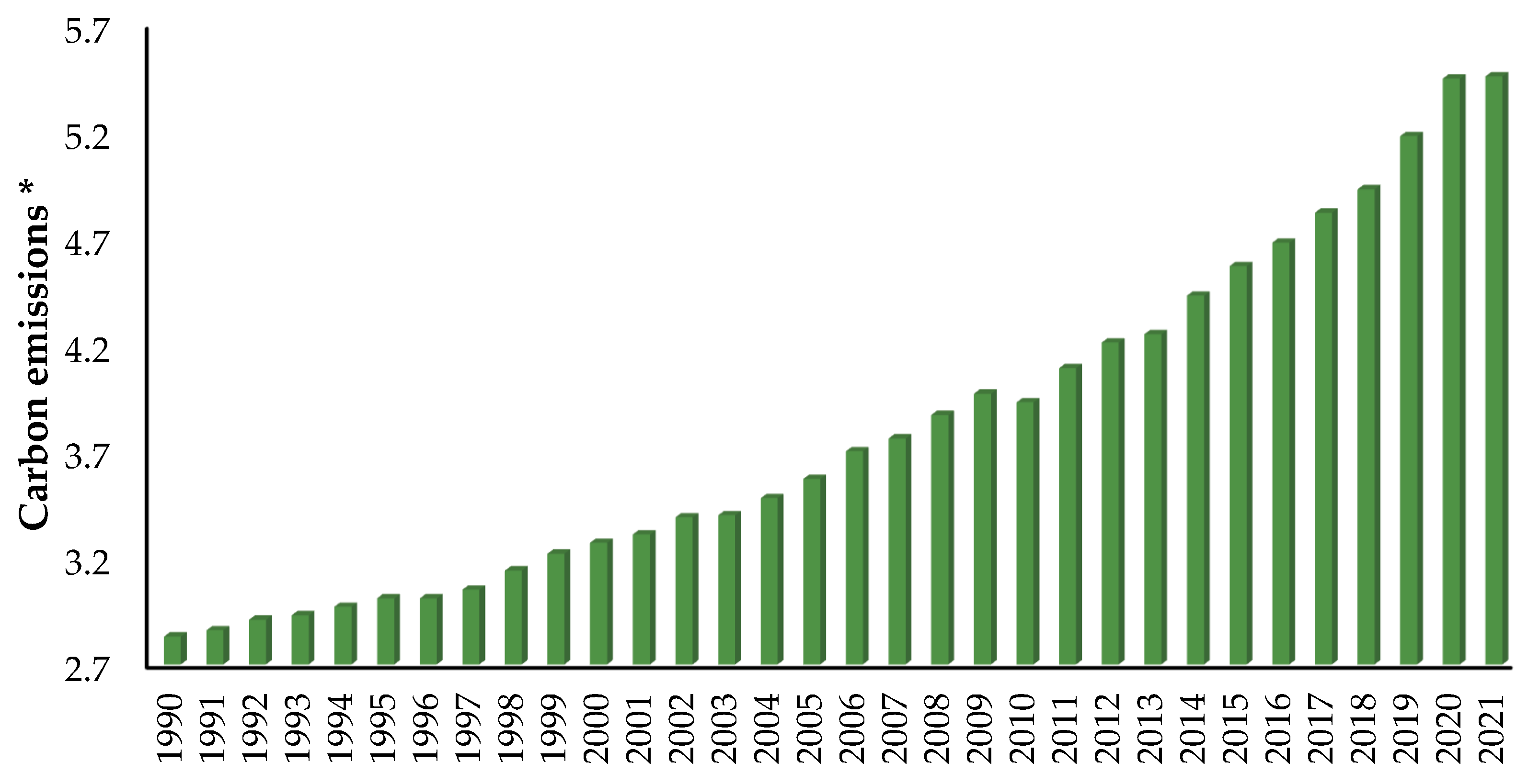
This study selected carbon emissions, especially those originating from energy, as environmental indicators because they are the most critical factors causing environmental pollution. An examination of OECD countries between 1990 and 2021 revealed that carbon emissions have generally been continuously increasing, except for 2020, because of the intensive use of fossil fuels. The period from 1990 to 2021 can be divided into 1990–1997 and 1998–2021. While it was 2.83 in 1990, it approximately doubled and reached 5.46 in 2021. Economic activities and energy consumption decreased significantly in 2020 due to the COVID-19 pandemic, resulting in a short-term decrease in carbon emissions. Carbon emissions increased again with the recovery of economic activities in 2021 (Figure 1).

2.2. Environmental Technology Dimension

While one dimension of the environment is energy, the other dimension is technology. Energy is an essential factor determining environmental impacts; while fossil fuels lead to high emissions, renewable energy sources are cleaner. Technology increases energy efficiency, contributes to reducing emissions, and improves the use of renewable energy. Effective management of energy and technology is critical to ensuring environmental sustainability.

While Schumpeter (1934) [12] stated that economic development is driven by innovation, Romer (1986) [13] emphasized the importance of R&D, human capital, and technological innovations. Energy technologies can potentially reduce environmental impacts and play an essential role in reducing dependence on fossil fuels and ensuring energy supply security. In addition, integrating technology and innovation into the energy sector can make energy production and consumption processes more efficient and environmentally friendly. Patents related to environmental technologies cover innovative solutions that promote environmental sustainability. These patents aim to reduce negative environmental impacts and encourage the use of greener technologies in various areas [12,13].

Energy technologies include innovations in various areas such as energy-efficient solutions (heat recovery and energy-saving devices), carbon capture and storage systems, environmentally friendly transportation technologies (electric and hybrid vehicles, hydrogen fuel cells), waste management and recycling methods, water and air purification systems, and sustainable agricultural practices (drip irrigation, organic fertilizers). These advances have LED to significant advances in environmental protection and sustainability.

The prominent inventions and patents in the field of environmental technologies are significant contributions to various areas aimed at increasing sustainability by offering innovative solutions. General Electric’s carbon capture system patent enables capturing and storing CO₂ emissions in industrial facilities. Toyota’s hybrid vehicle patents increase fuel efficiency and reduce emissions by combining gasoline and electric engines. Honda’s hydrogen fuel cell patent contributed to the spread of zero-emission vehicles. Tesla’s battery management system patent aims to extend the life of electric vehicle batteries and increase energy efficiency. Solyndra’s cylindrical solar panel patent offers panels that capture sunlight from a wider area. Siemens’ direct drive wind turbine patents increase turbine efficiency while reducing maintenance costs. These patents provide significant advances in environmental protection and sustainability. Investments in environmental technologies and patents in this area help both industries and individuals adopt more environmentally friendly solutions.

In particular, patents and technological inventions lead to revolutionary changes in the energy sector. New energy production methods, energy storage solutions, and technologies that increase energy efficiency are critical in shaping future energy systems. These innovations reduce environmental impacts, stimulate economic growth, create new jobs, increase employment, and support social well-being.

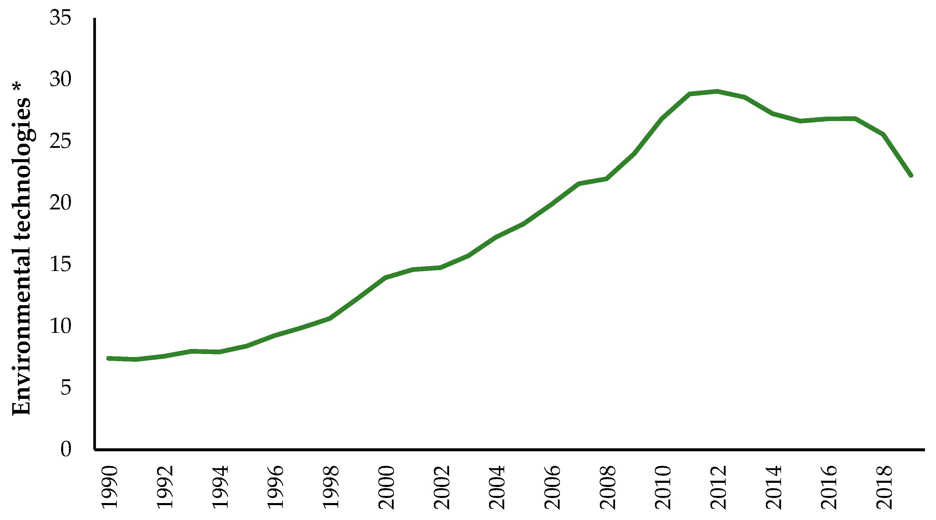
Technological inventions related to the environment are decreasing worldwide, and the share of OECD countries in these inventions is relatively low. Until 1994, the rates of per capita and local inventions remained at the same levels, but after 1994, the share of inventions per capita increased and reached its highest levels in 2012 (Figure 2).

The acceleration of technological advances can explain the increase in the share of inventions per capita after 1994, the increase in R&D investments, and the impact of innovation incentive policies. The fact that inventions per capita reached their highest levels in 2012 can be attributed to the increasing awareness of environmental technologies and the search for solutions to problems such as global warming and environmental pollution. During this period, significant progress was made in areas such as renewable energy sources, energy efficiency, and environmentally friendly technologies.

However, the fact that technological inventions related to the environment have decreased slightly in recent years indicates the need for new strategies. This decline may be due to a lack of financing, market uncertainties, regulatory barriers, or difficulties in commercializing innovative technologies. Moreover, the low share of OECD countries in these inventions reveals that these countries need to review their innovation policies and invest more in environmental technologies. To achieve sustainable development goals and effectively combat environmental problems in the future, encouraging and disseminating environmental technological inventions is highly important. In this context, international collaboration, public–private partnerships, and innovative financing models can accelerate the development and adoption of environmental technologies.

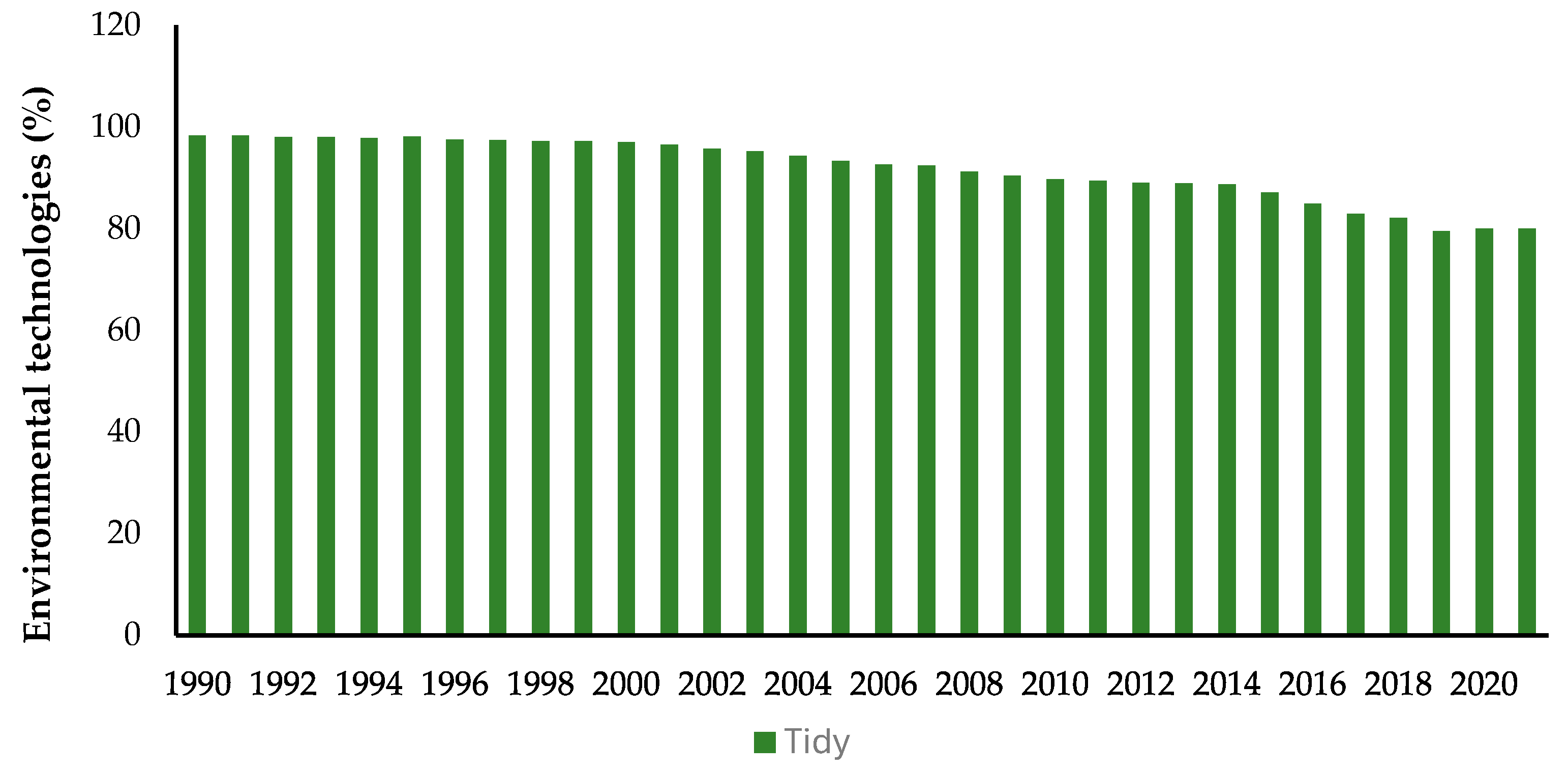
While the number of inventions related to the environment in 1990 was 98%, the fact that it decreased to 80% in 2021 does not mean that it decreased in environmental technologies. Environmental technologies grow more slowly than in other fields. Environment-related technologies are classified according to the environment. For example, electric vehicles in transportation, smart networks in energy, and sensitive irrigation systems in agriculture are both internal and environmental innovations. Such hybrid technologies may be effective in not increasing the percentage when it is not coded as an environmental invention in the classification.

From 1990 to 2021, there was no increase in the growth rate, expansion of the innovation universe, or diversification of the classification. It is clear that environmental technologies are integrated with other sectors, and that environmental innovation develops more in cross areas; thus, direct measurement will become increasingly complex.

On the other hand, in the 2020s, the focus of innovation was directed to health systems under the influence of digital transformation, blockchain, space technology, and the COVID-19 pandemic. The explosion of inventions in these areas may overshadow the proportional visibility of environmental technology (Figure 3).

When the period from 1990 to 2021 is examined, remarkable trends in the number of patents are observed. The number of patents sharply declined in 2018 and became even more pronounced in 2020. There was no significant increase in the number of patents up to 2018, and the curve generally followed a stable trend (Figure 4).

The stagnation during this period can be attributed to various factors. For example, factors such as economic recessions, insufficient innovation incentives, or pauses in technological developments may have prevented the increase in patent applications. However, the sharp declines in 2018, especially in 2020, may be associated with more specific events or policies. These declines may result from global economic crises, extraordinary situations such as pandemics, or changing legal and regulatory frameworks.

2.3. Energy Efficiency Dimension

Increasing energy efficiency contributes to the fight against global climate change. First, reducing energy consumption directly translates into fewer carbon emissions. This indicates that energy efficiency will be critical in future energy and climate change policies. Second, cost-effective energy efficiency can reduce the economic burden of achieving climate policy goals while providing environmental benefits at a low cost [14,15]. However, more efficient use of energy resources can also be associated with high levels of economic growth. This situation reveals energy efficiency’s critical environmental and economic advantages for sustainable development.

Energy efficiency generally has a positive effect on reducing carbon emissions. However, in some cases, negative effects can also occur. When energy efficiency increases, energy use can increase as energy costs decrease. This phenomenon is called the rebound effect [16]. The rebound effect, first proposed by Stanley Jevons (1865), is also known as the Jevons paradox. Jevons (1865), in his study on the British economy, stated that the effective operation of steam engines reduced coal consumption. However, these reductions in coal consumption reduce coal prices, increase coal demand, and increase coal consumption [17]. According to Greening et al. (2000), there are three main types of energy rebound effects: direct, indirect, and economy-wide effects [18]. However, Gavaskar and Geyer (2010) stated that while the direct rebound effect is microeconomic, indirect and economy-wide rebound effects are macroeconomic in size [19]. As energy efficiency increases, energy costs decrease, which can lead to an increase in energy demand. When the price decreases, energy demand increases again, and this cycle leads to the undermining of the efficiency provided; thus, the starting point is returned [20]. For example, using an energy-efficient appliance reduces energy costs, and consumers can direct these savings to other energy-intensive activities. As a result, total energy consumption increases; thus, carbon emissions may also increase. This cycle reduces the environmental benefits sought from energy efficiency and may prevent achieving emissions reduction targets in the long term.

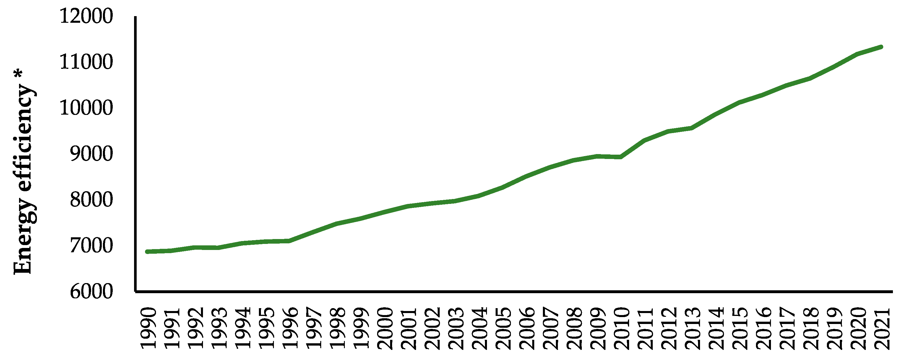
The energy efficiency curve exhibited a constant upward trend between 1990 and 2021. The slope of the curve did not increase much between 1990 and 1996; that is, there was no significant change in energy efficiency. The stable trend during this period may be because energy-efficient technologies have not yet been widely adopted or implemented (Figure 5).

After 1997, the slope of the energy efficiency curve began to increase significantly. Various factors can explain the increase during this period. In particular, the increasing interest in environmental sustainability and energy-saving issues since the late 1990s has led governments and the private sector to invest more in energy-efficient technologies. In addition, rising energy costs and awareness of the environmental impacts of fossil fuels have encouraged the widespread use of energy efficiency measures.

In the 2000s, with the development of energy-efficient technologies and the increased adoption of renewable energy sources, the energy efficiency curve accelerated even further. The tightening of energy efficiency standards and regulations, the introduction of innovative energy-saving solutions, and the financial incentives for energy efficiency projects contributed to the increase in the slope of the energy efficiency curve during this period.

Efforts toward energy efficiency continued in the 2010s, and policies aimed at optimizing energy consumption in developed countries became more intense. Applications such as intelligent energy management systems, energy-efficient buildings, and improved industrial processes have continuously increased energy efficiency. This process continues in parallel with awareness of energy efficiency and technological advances (Figure 5).

2.4. Dimension of Tax Revenues on Energy

Energy tax revenues significantly impact economic growth and carbon emissions. These taxes are essential for reducing carbon emissions and making energy consumption more sustainable.

Energy taxes make the use of fossil fuels more expensive. Regulations such as carbon taxes and energy taxes are designed to reduce carbon emissions. These taxes encourage businesses and individuals to shift to more environmentally friendly and cleaner energy sources. This orientation can increase the adoption of renewable energy technologies and improve energy efficiency, thereby reducing total carbon emissions. The design and implementation of tax policies play critical roles in balancing these two goals. A well-designed tax policy can promote sustainable energy use while supporting economic growth and reducing environmental impacts. According to the Environmental Kuznets Curve (EKC) hypothesis, there is a nonlinear relationship between economic growth and environmental degradation. This relationship suggests that economic growth may initially lead to environmental degradation, but after a certain threshold, environmental quality may improve [21,22]. In this context, energy taxes can support this process as a tool to reduce emissions. Energy taxes can reduce fossil fuel use and encourage the transition to renewable energy sources. These taxes can reduce the environmental impacts of production processes by increasing the cost of energy consumption. As a result, energy taxes can accelerate the achievement of the turning point in the EKC hypothesis and increase environmental sustainability.

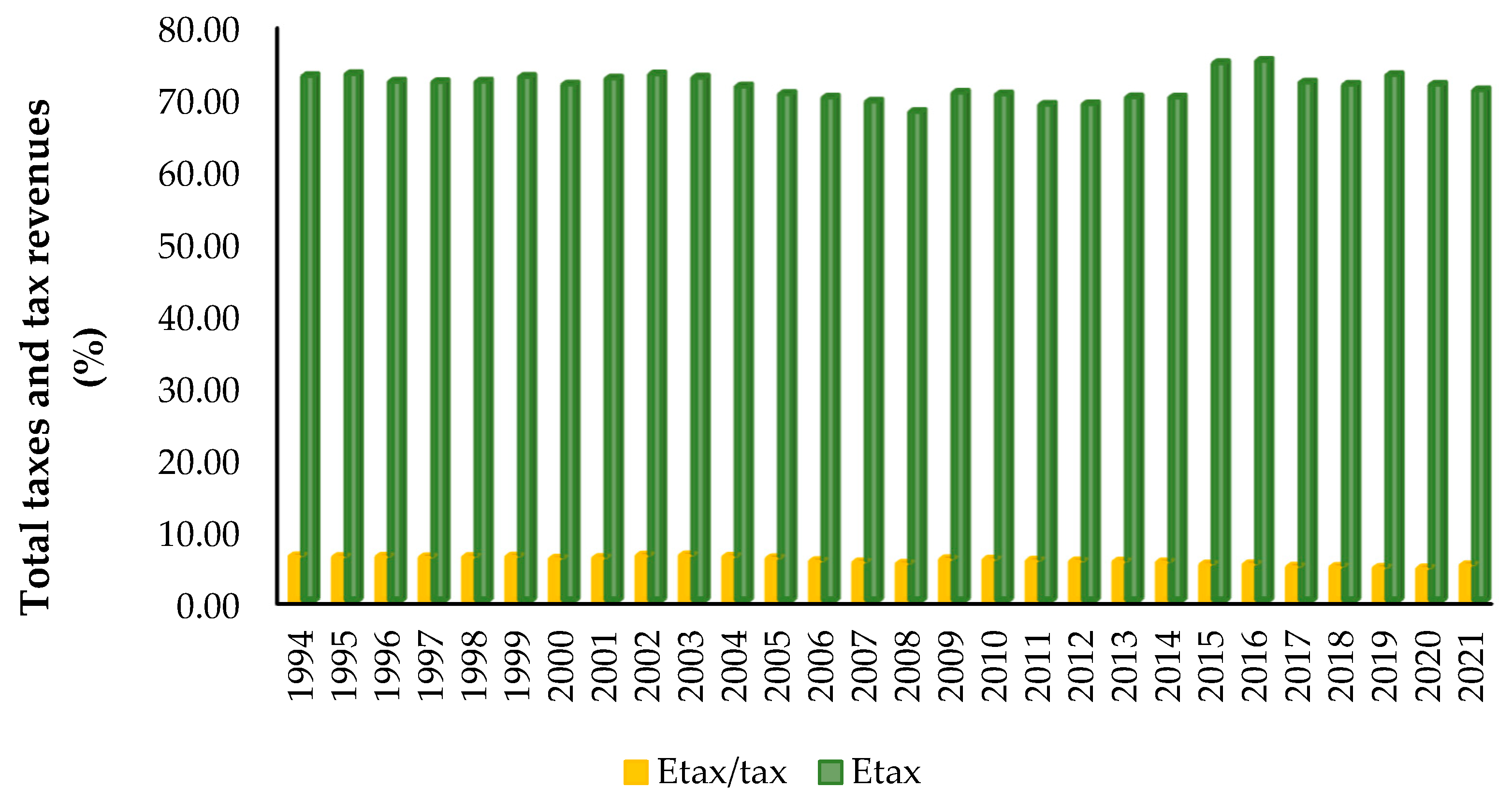
A graph of two variables shows the ratio of taxes collected on energy to total taxes and tax revenues collected on energy. The graph shows that taxes collected on energy are quite low compared with total taxes and that these values did not change much between 1990 and 2021 (Figure 6).

There may be several reasons why the share of energy taxes in total tax revenues remained low during this period. Governments may have limited such taxes, considering the potential negative effects of increasing energy taxes on economic growth and energy consumption.

Another reason is that a large portion of total tax revenues is obtained from other types of taxes, such as income taxes, corporate taxes, and value-added taxes. Therefore, energy taxes constitute a relatively low share of total tax revenues. Another reason why energy taxes remain low may be the increased use of renewable energy sources and the decrease in fossil fuel use. Incentives and support for renewable energy resources may have reduced the impact of taxes applied to fossil fuels.

3. Econometric Metrology

In real life, as in the simple linear regression equation above, it is not only X that explains Y; it is unrealistic to explain a phenomenon with a single equation system. However, in practice, econometric models are generally built on a single equation system, even though they have equations with more than one independent variable.

$${\mathrm{Y}}_{\mathrm{t}}=\propto +\beta {\mathrm{X}}_{\mathrm{t}}+{\epsilon }_{\mathrm{t}}$$

(1)

Understanding some of a system’s dynamics with a single equation is possible. Multivariate and multi-equation approaches should be adopted to perform more realistic and accurate analyses. Dynamics in the real world can usually be explained with more comprehensive and versatile models, such as simultaneous equation systems. These models allow for accurate predictions to be made simultaneously by considering the interaction of multiple internal and external variables.

$${\mathrm{X}}_{\mathrm{t}}=\propto +\delta {\mathrm{Z}}_{\mathrm{t}}+{\epsilon }_{\mathrm{t}}$$

(2)

Another variable, for example, Z, may not directly affect Y but may cause Y through X. Here, the simultaneous equation system can provide an effective solution for estimating the indirect effect. The direct impact on Y is estimated simultaneously with X; the indirect effect is estimated simultaneously with Z.

Suppose an endogenous variable in the system is used as an explanatory variable in any equation. In that case, a nonzero covariance may exist between the explanatory variable and the error term in that equation. This violates the assumption of cov(u, X) = 0. In this case, the estimates made via the least squares (OLS) method cannot be expected to be efficient, consistent, and unbiased. In addition, the existence of a relationship between independent variables (multiple linear correlations) prevents accurate estimates [23,24,25].

In such cases, it is necessary to estimate with simultaneous equation systems that handle multiple dependent variables defined by different equations within a system consisting of many equations [26]. The endogenous variable included in any equation of the simultaneous equation model may be included as an exogenous variable in another equation. In summary, simultaneous equation systems are systems consisting of more than one equation, where a variable is both a dependent (internal) variable explained by other variables and an independent (external) variable explaining them in the equation system, and where the variables interact with each other simultaneously (at the same time).

Simultaneous equation systems analyze electrical circuits, model static and dynamic systems, force balance, fluid dynamics, algorithm development, and data analysis estimations. Econometric models are generally used to analyze how many variables in the economy interact with each other. For example, the supply and demand equations can be estimated with a simultaneous equation system in an economic model. Since supply and demand affect each other, the price variables can be included in both equations as dependent and independent variables. In this case, there is a relationship in which price determines both supply and demand, and supply and demand determine the price.

Determining the internal and external variables in simultaneous equation systems is crucial for correctly estimating the model. The simultaneous equation system with the variables used in this study is modeled as follows. The variables used in this research and the econometric methods are explained to avoid repetition. Equations (3) and (4) show the structural equations of the simultaneous equation model, and ∝ β represents the structural parameters.

$${\mathrm{c}\mathrm{o}}_2={\propto }_0+{\propto }_1{\mathrm{g}\mathrm{d}\mathrm{p}}_{\mathrm{t}}+{\propto }_2{\mathrm{p}\mathrm{o}\mathrm{p}}_{\mathrm{t}}+{\propto }_3{\mathrm{e}\mathrm{p}}_{\mathrm{t}}+{\propto }_4{\mathrm{e}\mathrm{i}}_{\mathrm{t}}+{\epsilon }_{1\mathrm{t}}$$

(3)

$${\mathrm{e}\mathrm{p}}_{\mathrm{t}}={\beta }_0+{\beta }_1{\mathrm{p}}_{\mathrm{t}}+{\beta }_2{\mathrm{t}\mathrm{i}}_{\mathrm{t}}+{\beta }_3{\mathrm{t}\mathrm{i}\mathrm{y}\mathrm{y}}_{\mathrm{t}}+{\beta }_4{\mathrm{t}\mathrm{i}\mathrm{d}\mathrm{y}}_{\mathrm{t}}{+\beta }_5{\mathrm{c}\mathrm{o}}_2+{\epsilon }_{2\mathrm{t}}$$

(4)

The variables used in the study were determined as co₂, production-based CO₂ productivity, gdp per unit of energy-related CO₂ emissions—US dollars per unit of CO₂; gdp, real gdp—US dollars, PPP converted, Constant prices, 2015; pop, population, ages 15–64—percent of population; ep, energy productivity, gdp per unit of TES—constant prices, 2015; ei, energy intensity per capita; p, patent–environment–related technologies–Index; ti, development of environmental technologies—inventions per 1000000 people; tiyy, development of environmental technologies—percentage of domestic inventions; tidy development of environmental technologies—percentage of environmental inventions worldwide; etax, energy-related taxes revenue.

Endogenous variables are random variables that mutually affect each other in the model and are determined within the system. Nonrandom exogenous variables are variables that are determined outside the system. Therefore, there is no relationship between them and the error term. Lagged endogenous and exogenous variables belong to previous periods in the system.

• Endogenous variables: co₂, gdp
• Exogenous variables: pop, ep, ei, p, ti, tiyy, tidy

Reduced forms, where the endogenous variables in the structural form are on the left (explained) and the exogenous variables are on the right (explanatory), are equations written to find the effect of previously determined variables on endogenous variables. In other words, there are equations obtained by solving the simultaneous structural equation for endogenous variables, as many reduced forms as the number of endogenous variables are obtained. The reduced-form coefficients are obtained by estimating the reduced-form equations.

The ep variable in Equation (4) was replaced by the ep variable in Equation (3) to obtain the reduced form of Equation (5), and its steps are shown below.

$${\mathrm{c}\mathrm{o}}_2={\propto }_0+{\propto }_1{\mathrm{g}\mathrm{d}\mathrm{p}}_{\mathrm{t}}+{\propto }_2{\mathrm{p}\mathrm{o}\mathrm{p}}_{\mathrm{t}}+{\propto }_3{\beta }_0+{{\propto }_3\beta }_1{\mathrm{p}}_{\mathrm{t}}+{{\propto }_3\beta }_2{\mathrm{t}\mathrm{i}}_{\mathrm{t}}+{{\propto }_3\beta }_3{\mathrm{t}\mathrm{i}\mathrm{y}\mathrm{y}}_{\mathrm{t}}+{{\propto }_3\beta }_4{\mathrm{t}\mathrm{i}\mathrm{d}\mathrm{y}}_{\mathrm{t}}+{{\propto }_3\beta }_5{\mathrm{c}\mathrm{o}}_2{{+\propto }_3\epsilon }_{2\mathrm{t}}+{\propto }_4{\mathrm{e}\mathrm{i}}_{\mathrm{t}}+{\epsilon }_{1\mathrm{t}}$$

(5)

$${\mathrm{c}\mathrm{o}}_2={\propto }_0+{\propto }_3{\beta }_0+{\propto }_1{\mathrm{g}\mathrm{d}\mathrm{p}}_{\mathrm{t}}+{\propto }_2{\mathrm{p}\mathrm{o}\mathrm{p}}_{\mathrm{t}}+{{\propto }_3\beta }_1{\mathrm{p}}_{\mathrm{t}}+{{\propto }_3\beta }_2{\mathrm{t}\mathrm{i}}_{\mathrm{t}}+{{\propto }_3\beta }_3{\mathrm{t}\mathrm{i}\mathrm{y}\mathrm{y}}_{\mathrm{t}}+{{\propto }_3\beta }_4{\mathrm{t}\mathrm{i}\mathrm{d}\mathrm{y}}_{\mathrm{t}}+{{\propto }_3\beta }_5{\mathrm{c}\mathrm{o}}_2{{+\propto }_3\epsilon }_{2\mathrm{t}}+{\propto }_4{\mathrm{e}\mathrm{i}}_{\mathrm{t}}+{\epsilon }_{1\mathrm{t}}$$

(6)

$$\begin{gathered} (1-{{\propto }_3\beta }_5{)\mathrm{c}\mathrm{o}}_2={\propto }_0+{\propto }_3{\beta }_0+{\propto }_1{\mathrm{g}\mathrm{d}\mathrm{p}}_{\mathrm{t}}+{\propto }_2{\mathrm{p}\mathrm{o}\mathrm{p}}_{\mathrm{t}}+{{\propto }_3\beta }_1{\mathrm{p}}_{\mathrm{t}}+{{\propto }_3\beta }_2{\mathrm{t}\mathrm{i}}_{\mathrm{t}}+{{\propto }_3\beta }_3{\mathrm{t}\mathrm{i}\mathrm{y}\mathrm{y}}_{\mathrm{t}}+{{\propto }_3\beta }_4{\mathrm{t}\mathrm{i}\mathrm{d}\mathrm{y}}_{\mathrm{t}}+{\propto }_4{\mathrm{e}\mathrm{i}}_{\mathrm{t}}{{+\propto }_3\epsilon }_{2\mathrm{t}}+{\epsilon }_{1\mathrm{t}} \\ {\left(1-{{\propto }_3\beta }_5\right)/\left(1-{{\propto }_3\beta }_5\right)\mathrm{c}\mathrm{o}}_2={\propto }_0+{\propto }_3{\beta }_0/\left(1-{{\propto }_3\beta }_5\right)+{\propto }_1/\left(1-{{\propto }_3\beta }_5\right){\mathrm{g}\mathrm{d}\mathrm{p}}_{\mathrm{t}}+{\propto }_2/\left(1-{{\propto }_3\beta }_5\right){\mathrm{p}\mathrm{o}\mathrm{p}}_{\mathrm{t}}+ \\ {{\propto }_3\beta }_1/\left(1-{{\propto }_3\beta }_5\right){\mathrm{p}}_{\mathrm{t}}+{{\propto }_3\beta }_2/\left(1-{{\propto }_3\beta }_5\right){\mathrm{t}\mathrm{i}}_{\mathrm{t}}+{{\propto }_3\beta }_3/\left(1-{{\propto }_3\beta }_5\right){\mathrm{t}\mathrm{i}\mathrm{y}\mathrm{y}}_{\mathrm{t}}+{{\propto }_3\beta }_4/\left(1-{{\propto }_3\beta }_5\right){\mathrm{t}\mathrm{i}\mathrm{d}\mathrm{y}}_{\mathrm{t}}+ \\ {\propto }_4/(1-{{\propto }_3\beta }_5){\mathrm{e}\mathrm{i}}_{\mathrm{t}}+{{\propto }_3\epsilon }_{2\mathrm{t}}+{\epsilon }_{1\mathrm{t}}/(1-{{\propto }_3\beta }_5) \end{gathered}$$

(7)

$${\mathrm{c}\mathrm{o}}_2={\pi }_0+{\pi }_1{\mathrm{g}\mathrm{d}\mathrm{p}}_{\mathrm{t}}+{\pi }_2{\mathrm{p}\mathrm{o}\mathrm{p}}_{\mathrm{t}}+{\pi }_3{\mathrm{p}}_{\mathrm{t}}+{\pi }_4{\mathrm{t}\mathrm{i}}_{\mathrm{t}}+{{\pi }_5\mathrm{t}\mathrm{i}\mathrm{y}\mathrm{y}}_{\mathrm{t}}+{{\pi }_6\mathrm{t}\mathrm{i}\mathrm{d}\mathrm{y}}_{\mathrm{t}}+{{\pi }_7\mathrm{e}\mathrm{i}}_{\mathrm{t}}+{\omega }_{\mathrm{t}}$$

(8)

Equation (5) shows the reduced form structure, which is the expression of the endogenous variable only as a function of the exogenous variables. Where π represents the structure parameters, these parameters have direct and indirect effects. ${\epsilon }_{1\mathrm{t}},{\epsilon }_{2\mathrm{t}}, \mathrm{a}\mathrm{n}\mathrm{d} {\omega }_{\mathrm{t}}$ represents the error terms.

There is no endogenous variable on the right side of the equation above. The OLS assumption is met since there will be no relationship between the independent variable(s) and the error term (${\omega }_{\mathrm{t}}$). In addition, since the relationship between the endogenous variables on the right side of the structural equation and the error terms is eliminated, the estimated values are unbiased.

3.1. Determination Conditions

Before estimating simultaneous equation systems, the equations must meet the determination conditions. In a simultaneous equation system, the condition of examining whether the estimates of the structural coefficient parameters of each structural equation can be obtained as a single value is called the determination condition [27].

For this, two conditions, namely, order and rank conditions, must be met.

i. Order condition: This is a necessary but insufficient condition for determining the equation of a simultaneous equation system. For an equation to be determined, the number of variables not included in this equation must be equal to or greater than one minus the number of endogenous variables of the model (K-M ≥ G-1) [23,28,29].

There are three possible situations. These situations are as follows:

I. Underdetermination: K-M < G-1

If structural coefficient parameter estimates of the structural equation, whose determination is examined in a simultaneous equation system, cannot be obtained, the structural equation will not be determined. In this case, the equation cannot be estimated.

II. Exact determination: K-M = G-1

The structural equation is wholly determined if precise estimates of the structural form coefficients can be obtained via the reduced form coefficients. Thus, equations can be estimated via instrumental variables, indirect least squares (DOLS), and two-stage least squares (2SLS) methods.

III. Overdetermination: K-M > G-1

If the structural coefficient parameter estimates of the structural equation, whose determination status is examined in a simultaneous equation system, yield more than one solution value, the structural equation is overdetermined. For determination, 2SLS and three-stage least squares (3SLS) methods should be preferred. In 2SLS, each equation in the model is estimated separately, whereas in 3SLS, all equations are estimated simultaneously. Table 1 presents the possible situations, conditions, and a summary of the methods that can be used.

• G: Total number of endogenous variables;
• K: Total number of variables (endogenous + exogenous) in the model;
• M: Total number of variables (endogenous + exogenous) in the equation.

Table 1. Determination conditions and methods.

Situation	Conditions	Explanation	Methods
Underdetermination	K-M < G-1	The equation is undetermined if the structural form coefficients cannot be obtained from the reduced form coefficients.	The equation cannot be estimated.
Overdetermination	K-M = G-1	If the structural form coefficients are obtained by using the reduced form coefficients, the equation is exactly determined.	DOLS, 2SLS, instrumental variable method
Exact determination	K-M > G-1	If more than one solution value is obtained for the structural equation coefficients, the equation is over-determined.	2SLS 3SLS

Source: Compiled by the author.

Table 1. Determination conditions and methods.

Situation	Conditions	Explanation	Methods
Underdetermination	K-M < G-1	The equation is undetermined if the structural form coefficients cannot be obtained from the reduced form coefficients.	The equation cannot be estimated.
Overdetermination	K-M = G-1	If the structural form coefficients are obtained by using the reduced form coefficients, the equation is exactly determined.	DOLS, 2SLS, instrumental variable method
Exact determination	K-M > G-1	If more than one solution value is obtained for the structural equation coefficients, the equation is over-determined.	2SLS 3SLS

Source: Compiled by the author.

ii. Rank condition: The rank condition, which is a sufficient condition, must be examined. The rank condition means that the rank of the matrix consisting of the parameters excluded from the equation under consideration is equal to (G-1), that is, one less than the total number of endogenous variables. The rank condition is called because it examines the largest square matrix whose determinant is not zero. According to the rank condition, the determination of the equation under consideration in a G equation model is only possible by forming at least one determinant different from zero, which is the number of rows and columns (G-1), from the coefficients of the variables not included in this equation but included in the other equations of the system. The coefficients of the variables not included in this equation but included in the system’s other equations are arranged so that they remain in the table, and the other coefficients are deleted (Tables 3–6).

3.2. Simultaneous Equation Systems

After the determination situation is examined, the method used to estimate simultaneous equation systems can be determined, and the estimation phase can be started. Systems of simultaneous equations are estimated via two and three-stage least squares, limited information maximum likelihood, complete information maximum likelihood, seemingly unrelated regressions (SUR), and generalized moments methods. Since the equations were overdetermined in this study, estimations were made with the 2SLS and 3SLS methods. Therefore, these two methods are discussed in detail below.

3.2.1. Two-Stage Least Squares Method

Theil (1953) and Basman (1957), independently of each other, developed the two-stage least squares method as a particular case of the generalized least squares method. The single-equation method, 2SLS, is a linear method that includes two separate estimations for all equations in a system of equations, as used in the estimation of instrumental variable models [30,31]. In cases where the estimators are related to the error term, and there is multicollinearity, 2SLS is a method used to estimate consistent structural parameter values in equations with exact and overdetermined values in simultaneous equation systems. It gives the same estimated values as DOLS in models with complete determination. The 2SLS method is applied in two steps:

Step 1: To eliminate the relationship between the endogenous variable Y_t and the error term w_t, Y_t is estimated according to the instrumental and exogenous variables in the equation. This estimation allows for Y_t to be determined independently of the error term. Thus, each endogenous variable is obtained with reduced form equations, with exogenous variables at this stage.

Step 2: In the structural equation to be estimated, instrumental variables replace the endogenous variables on the right side, and a transformed structural equation is obtained [32]. Thus, an estimate that is not related to the error terms is obtained by using instrumental variables. Equations with consistent parameters and no correlation between the endogenous variables and error terms are estimated.

Two-stage least squares estimators: These estimators are asymptotically unbiased (2SLS is more suitable for large samples; it may yield deviant estimates in small samples) and asymptotically efficient [33,34]. It is also easy to calculate and produces good results. On the other hand, it is sensitive to specification errors, and in cases where there are many exogenous variables, the sample size should be large. If the coefficients of determination of the reduced form equations are high, OLS and 2SLS estimates may be close to each other.

Assumptions of the two-stage least squares method: The estimated error term of the structural equation has zero mean, equal variance, and no autocorrelation.

• The reduced-form error terms also have a zero mean, equal variance, no autocorrelation, and no correlation with exogenous variables.
• There is no multicollinearity between exogenous variables.
• The model is correctly established in terms of exogenous variables.
• The sample size is greater than the total number of exogenous variables in the structural model. Significantly reduced-form parameters cannot be estimated if the sample size is smaller than the number of exogenous variables.

3.2.2. Three-Stage Least Squares Method

This method was developed by Theil (1953) and Zellner (1962) to continue Theil’s two-stage least squares method. The three-stage least squares method (3SLS) is combined with the seemingly unrelated regression (SUR) method with the two-stage least squares (2SLS) [30,35,36]. SUR is a generalization of the linear regression model consisting of various regression equations. The 3SLS method is estimated by repeating the least squares method in three successive stages. These steps are as follows:

Step 1: Reduced-form equations are estimated for each endogenous variable in the model, and the estimated values of the endogenous variables are found.

Step 2: In the structural equations, the endogenous variables on the right side are replaced by instrumental variables, and transformed structural equations are obtained. The two-stage least squares estimators of the structural parameters are found by applying the least squares method (OLS) to the transformed equations.

Step 3: By applying the generalized least squares method, or, in other words, by using the least squares method to the transformed equations, the estimated values are re-estimated together. Thus, the three-stage least squares estimators of the structural parameters are estimated.

In three-stage least squares estimation, all model equations are estimated simultaneously, and the estimates are asymptotically efficient and consistent [24,34]. The advantage of 3SLS is that it allows for the simultaneous estimation of all the model parameters. It considers a possible correlation between the error terms of the structural form of the model. 3SLS estimators are more efficient than 2SLS estimators. While it obtains consistent estimators for a large sample, it may be biased for small samples [37]. Similarly, the 3SLS method addresses not only any endogeneity and simultaneity problems but also any correlation between the error terms of the equation system.

4. Econometric Analysis Results

4.1. Variables and Dataset

This study’s environmental, energy, environmental technologies, and economic dimensions were estimated via simultaneous equation systems and monthly data for OECD countries between 1990 and 2021. The data was compiled from the OECD database.

Models were created with variables that may cause carbon dioxide emissions. These variables include energy-related carbon dioxide emissions (co₂), gross domestic product (gdp), population (pop), energy efficiency (ep), energy intensity (ei), environmental technological patents (p), inventions per capita (ti), the percentage of domestic inventions (tiyy), the percentage of worldwide inventions (tidy), and energy-related tax revenue (etax). All the variables used in this study and their explanations are presented in Table 2. Double logarithmic (log–log) models of regression coefficients were used to estimate the elasticity of the variables directly.

Before the models were estimated, the stationarity of the variables was examined, and the co₂, gdp, ep, ei, and etax variables are stationary in the first difference; pop, p, ti, tiyy, and tidy variables are stationary in the second difference. The results of the stationarity test are shown in Appendix A,

Table A1. Phillips–Perron Test.

Variable	Level	First Difference	Second Difference
co2	−1.138201	−4.480200
gdp	−1.217730	−4.331756
pop	1.331310	−1.395251	−19.21044
ep	−2.759151	−4.342206
ei	−1.352727	−4.595089
p	14.11781	0.906659	−19.28744
ti	2.821285	−1.929907	−18.67615
tiyy	−0.238021	−1.074882	−18.58010
tidy	1.989226	−2.858455	−18.56739
etax	−1.928550	−4.054032

The 1%, 5%, and 10% significance levels are −3.98, −3.42, and −3.13, respectively.

.

Table 2. Variables and their explanations.

Variables	Explanations	Variables	Explanations
co2	Production-based CO2 productivity	p	Patent–Environment-Related Technologies-Index
gdp	per unit of energy-related CO2 emissions-US dollars per unit of CO2	ti	Development of environmental technologies-inventions per 1,000,000 people
pop	Population, ages 15-64-Percentage of population	tiyy	Development of environmental technologies-percentage of domestic inventions
ep	Energy productivity, gdp per unit of TES-constant prices, 2015	tidy	Development of environmental technologies-percentage of environmental inventions worldwide
ei	Energy intensity per capita	etax	Energy-related tax revenue

Table 2. Variables and their explanations.

Variables	Explanations	Variables	Explanations
co2	Production-based CO2 productivity	p	Patent–Environment-Related Technologies-Index
gdp	per unit of energy-related CO2 emissions-US dollars per unit of CO2	ti	Development of environmental technologies-inventions per 1,000,000 people
pop	Population, ages 15-64-Percentage of population	tiyy	Development of environmental technologies-percentage of domestic inventions
ep	Energy productivity, gdp per unit of TES-constant prices, 2015	tidy	Development of environmental technologies-percentage of environmental inventions worldwide
ei	Energy intensity per capita	etax	Energy-related tax revenue

4.2. Development of Alternative Models

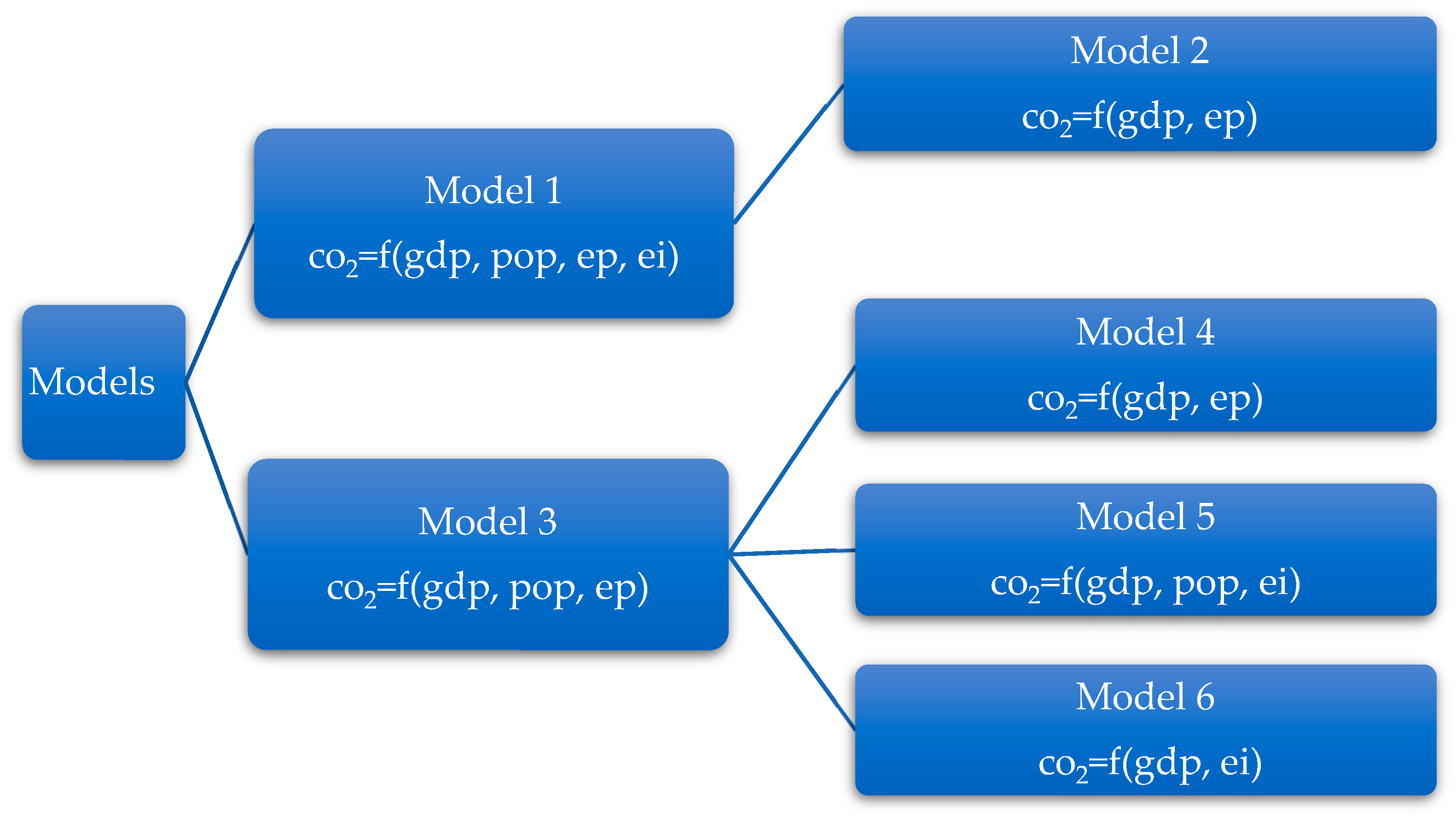
The primary research focus of this study is to examine carbon dioxide emissions, which stand out for their profound effects on the environment and environmental pollution. The main reason for reviewing carbon emissions is that they are a focal point in discussions on environmental protection and sustainable development. In this context, two main models and four submodels were created. While the first primary model includes models related to environmental, technological, and environmental technological inventions, the second primary model focuses on taxes on energy. Since there are too many variables and models, the functions and models used in this study are summarized in Figure 7 to avoid confusion.

4.2.1. Models Consisting of Patents and Inventions Related to Environmental Technologies

This section consists of a basic model and a submodel. After Model 1 was estimated, the insignificant variables (pop and ei) were removed from the model, and Model 2 was created.

co₂ = f(gdp, pop, ep, ei) (Model 1)

ep = f(p, ti, tiyy, tidy)

$${\mathrm{c}\mathrm{o}}_2={\propto }_0+{\propto }_1{\mathrm{g}\mathrm{d}\mathrm{p}}_{\mathrm{t}}+{\propto }_2{\mathrm{p}\mathrm{o}\mathrm{p}}_{\mathrm{t}}+{\propto }_3{\mathrm{e}\mathrm{p}}_{\mathrm{t}}+{\propto }_4{\mathrm{e}\mathrm{i}}_{\mathrm{t}}+{\epsilon }_{1\mathrm{t}}$$

(9)

$${\mathrm{e}\mathrm{p}}_{\mathrm{t}}={\beta }_0+{\beta }_1{\mathrm{p}}_{\mathrm{t}}+{\beta }_2{\mathrm{t}\mathrm{i}}_{\mathrm{t}}+{\beta }_3{\mathrm{t}\mathrm{i}\mathrm{y}\mathrm{y}}_{\mathrm{t}}+{\beta }_4{\mathrm{t}\mathrm{i}\mathrm{d}\mathrm{y}}_{\mathrm{t}}{+\beta }_5{\mathrm{c}\mathrm{o}}_2+{\epsilon }_{2\mathrm{t}}$$

(10)

• Exogenous variables: pop, ep, ei, p, ti, tiyy, tidy, etax
• Endogenous variables: co₂, gdp

For the model to be estimated correctly, each exogenous variable must be selected correctly, and there must be no multicollinearity among them. Therefore, it is necessary to test the relationships between exogenous variables. The Variance Inflation Factor (VIF) test was used to check whether there was a problem of multiple linear correlations between exogenous variables. The null hypothesis of no multicollinearity cannot be rejected in the models. Therefore, there is no multilinear correlation between exogenous variables (Appendix A,

Table A2. Variance Inflation Factors.

	Coefficient	Uncentered	Centered
Variable	Variance	VIF	VIF
DDLTI	0.002127	1.291665	1.290434
DDLTIYY	0.003950	1.229684	1.226679
DDLTIDY	0.072434	1.070945	1.068596

). Before proceeding with the estimation, the determination conditions were examined. The determination conditions of the structural equation of Model 1 are given below:

According to the order condition,

• For structural Equation (9):

9–5~2–1

4 > 1 over identified

• For structural Equation (10):

9–6~2–1

3 > 1 over identified

The model to be used was determined according to the determination conditions of the system. The model examined is overdetermined. In this case, the methods that can be used are 2SLS, instrumental variables, and 3SLS. The 2SLS and instrumental variable methods are single equation methods, whereas the 3SLS method is a system method. In Model 1, all the equations satisfy the necessary order condition. In the second stage, the rank condition, which is a sufficient condition, was researched.

In the simultaneous equation system, all variables on the right side of each equation, except for the error terms, were placed on the left side of the equation. Then, for each equation on the left side, all variables that exist or do not exist in the model were written with their structural coefficients. With this arrangement, a table was prepared for the structural coefficient parameters.

In the prepared table, the entire row of the equation under examination was deleted, and all values in the column where the variables with zero coefficient parameters (except themselves) were written in the deleted equation. The equation under examination was determined if there were M-1 nonzero rows and columns among the written values. The rank condition, which expresses the obtained coefficient matrix, was prepared for Model 1 and is shown in Table 3 and Table 4.

$${\mathrm{c}\mathrm{o}}_2{-\propto }_0-{\propto }_1{\mathrm{g}\mathrm{d}\mathrm{p}}_{\mathrm{t}}-{\propto }_2{\mathrm{p}\mathrm{o}\mathrm{p}}_{\mathrm{t}}-{\propto }_3{\mathrm{e}\mathrm{p}}_{\mathrm{t}}-{\propto }_4{\mathrm{e}\mathrm{i}}_{\mathrm{t}}={\epsilon }_{1\mathrm{t}}$$

(11)

$${\mathrm{e}\mathrm{p}}_{\mathrm{t}}-{\beta }_0-{\beta }_1{\mathrm{p}}_{\mathrm{t}}-{\beta }_2{\mathrm{t}\mathrm{i}}_{\mathrm{t}}-{\beta }_3{\mathrm{t}\mathrm{i}\mathrm{y}\mathrm{y}}_{\mathrm{t}}-{\beta }_4{\mathrm{t}\mathrm{i}\mathrm{d}\mathrm{y}}_{\mathrm{t}}{-\beta }_5{\mathrm{c}\mathrm{o}}_2={\epsilon }_{2\mathrm{t}}$$

(12)

Table 3. Matrix of Model 1.

Equations	Variables
	co2	gdp	pop	ep	ei	p	ti	tiyy	tidy
I. Equations	1	$-{\propto }_1$	$-{\propto }_2$	$-{\propto }_3$	$-{\propto }_4$	0	0	0	0
II. Equations	$-{\beta }_5$	0	0	1	0	${-\beta }_1$	$-{\beta }_2$	$-{\beta }_3$	$-{\beta }_4$

Table 3. Matrix of Model 1.

Equations	Variables
	co2	gdp	pop	ep	ei	p	ti	tiyy	tidy
I. Equations	1	$-{\propto }_1$	$-{\propto }_2$	$-{\propto }_3$	$-{\propto }_4$	0	0	0	0
II. Equations	$-{\beta }_5$	0	0	1	0	${-\beta }_1$	$-{\beta }_2$	$-{\beta }_3$	$-{\beta }_4$

$$\Delta =\left|{-\beta }_1-{\beta }_2{-\beta }_3-{\beta }_4\right|\ne 0$$

Table 4. Matrix of Model 1.

Equations	Variables
	co2	gdp	pop	ep	ei	p	ti	tiyy	tidy
I. Equations	1	$-{\propto }_1$	$-{\propto }_2$	$-{\propto }_3$	$-{\propto }_4$	0	0	0	0
II. Equations	$-{\beta }_5$	0	0	1	0	${-\beta }_1$	$-{\beta }_2$	$-{\beta }_3$	$-{\beta }_4$

Table 4. Matrix of Model 1.

Equations	Variables
	co2	gdp	pop	ep	ei	p	ti	tiyy	tidy
I. Equations	1	$-{\propto }_1$	$-{\propto }_2$	$-{\propto }_3$	$-{\propto }_4$	0	0	0	0
II. Equations	$-{\beta }_5$	0	0	1	0	${-\beta }_1$	$-{\beta }_2$	$-{\beta }_3$	$-{\beta }_4$

$$\Delta =\left|{-\alpha }_1-{\alpha }_2-{\alpha }_4\right|\ne 0$$

This matrix satisfies the rank condition, which is a sufficient condition for Equations (11) and (12), since the determinant of at least one matrix with the number of rows and columns G-1 is different from zero; thus, there is no problem of determination.

4.2.2. Models Consisting of Tax Revenues on Energy

Model 3 was established to examine whether tax revenues on energy indirectly affect carbon emissions through gdp. As in Model 1, the determination conditions were first examined.

co₂ = f(gdp, pop, ep, ei)

gdp =f (etax, co₂)

$${\mathrm{c}\mathrm{o}}_2={\propto }_0+{\propto }_1{\mathrm{g}\mathrm{d}\mathrm{p}}_{\mathrm{t}}+{\propto }_2{\mathrm{p}\mathrm{o}\mathrm{p}}_{\mathrm{t}}+{\propto }_3{\mathrm{e}\mathrm{p}}_{\mathrm{t}}+{\epsilon }_{\mathrm{t}}$$

(13)

$${\mathrm{g}\mathrm{d}\mathrm{p}}_{\mathrm{t}}={\beta }_0+{\beta }_1{\mathrm{e}\mathrm{t}\mathrm{a}\mathrm{x}}_{\mathrm{t}}+{{\beta }_2{\mathrm{c}\mathrm{o}}_2+\epsilon }_{\mathrm{t}}$$

(14)

According to the order condition,

• For structural Equation (13):

9–4~2–1

5 > 1 over identified

• For structural Equation (14):

9–3~2–1

6 > 1 over identified

In Model 3, over-identification is observed, and all the equations satisfy the order condition. In the second stage, the sufficient and rank conditions were investigated, and the rank condition, which is an acceptable condition, was investigated.

Since the equations’ determinants’ matrices differ from zero, the equations have no determination problem. The determination situations in Models 1 and 3 are explained in detail above. Table 5 and Table 6 present the order and rank conditions of the other four models. These four models meet both the order and rank conditions, so there is no determination problem.

Table 5. Matrix of Model 3.

Equations			Variables
	co2	gdp	pop	$\mathbf{e}\mathbf{p}$	$\mathbf{e}\mathbf{t}\mathbf{a}\mathbf{x}$
I. Equations	1	$-{\propto }_1$	$-{\propto }_2$	$-{\propto }_3$	$0$
II. Equations	0	0	0	0	${-\beta }_1$

Table 5. Matrix of Model 3.

Equations			Variables
	co2	gdp	pop	$\mathbf{e}\mathbf{p}$	$\mathbf{e}\mathbf{t}\mathbf{a}\mathbf{x}$
I. Equations	1	$-{\propto }_1$	$-{\propto }_2$	$-{\propto }_3$	$0$
II. Equations	0	0	0	0	${-\beta }_1$

$$\Delta =\left|{-\beta }_1\right|\ne 0$$

Table 6. Matrix of Model 3.

Equations			Variables
	co2	gdp	pop	$\mathbf{e}\mathbf{p}$	$\mathbf{e}\mathbf{t}\mathbf{a}\mathbf{x}$
I. Equations	1	$-{\propto }_1$	$-{\propto }_2$	$-{\propto }_3$	$0$
II. Equations	0	0	0	0	${-\beta }_1$

Table 6. Matrix of Model 3.

Equations			Variables
	co2	gdp	pop	$\mathbf{e}\mathbf{p}$	$\mathbf{e}\mathbf{t}\mathbf{a}\mathbf{x}$
I. Equations	1	$-{\propto }_1$	$-{\propto }_2$	$-{\propto }_3$	$0$
II. Equations	0	0	0	0	${-\beta }_1$

$$\Delta =\left|-{\alpha }_2{-\alpha }_3\right|\ne 0$$

As a result, it is seen that the equations of all models (6) satisfy the (2) order condition. As a result, the equations of all the models (6) meet the (2) order condition, and there is overdetermination. In this case, the equations can be estimated through the 2SLS and 3SLS methods. The determinant values of the matrices obtained from both equations of the six models meet sufficient conditions since they are different from 0 (

Table 7. Order and rank conditions of the models.

		Order Condition		Rank Condition	$\Delta \ne 0$
Model 2	1. Equations	6 > 1	Over Identified	$\Delta =\left|{-\beta }_1-{\beta }_2{-\beta }_3-{\beta }_4\right|$
	2. Equations	3 > 1		$\Delta =\left|{-\alpha }_1-{\alpha }_2-{\alpha }_4\right|$
Model 4	1. Equations	6 > 1		$\Delta =\left|{-\beta }_1\right|$
	2. Equations	6 > 1		$\Delta =\left|-{\alpha }_2\right|$
Model 5	1. Equations	5 > 1		$\Delta =\left|{-\beta }_1\right|$
	2. Equations	6 > 1		$\Delta =\left|-{\alpha }_2-{\alpha }_3\right|$
Model 6	1. Equations	6 > 1		$\Delta =\left|{-\beta }_1\right|$
	2. Equations	6 > 1		$\Delta =\left|-{\alpha }_2\right|$

).

5. Econometric Estimations and Results

Since all the equations are overidentified, estimations were made through the 2SLS and 3SLS methods. In this subsection, the estimation results are presented in

Table 8. Estimates of a system of simultaneous equations via two-stage and three-stage least squares.

	2SLS				3SLS
	gdp	pop	ep	ei	gdp	pop	ep	ei
Model 1	0.10 0.0650	−0.11 0.0096	0.13 0.0246	−0.39 0.0366	0.14 0.0020	−0.05 0.1201	0.08 0.1013	−0.21 0.1595
Instruments: p, ti, tiyy, tidy, and co2
	R2 = 0.50				R2 = 0.32
Model 2					0.27 0.0000		−0.05 0.0550
	R2 = 0.23				R2 = 0.23
Model 3	−0.15 0.0002	34.26 0.8416	0.41 0.0000		−0.15 0.0022	34.26 0.7705	0.41 0.0001
Instruments: etax and co2
	R2 = 0.42				R2 = 0.42
Model 4	−0.15 0.0001		0.40 0.0000		−0.15 0.0023		0.40 0.0000
	R2 = 0.45				R2 = 0.45
Model 5	−0.15 0.0834	−455.15 0.1515		−0.89 0.0494	−0.15 0.0022	−455.15 0.2125		−0.89 0.0297
Instruments: etax and co2
	R2 = 0.02				R2 = 0.02
Model 6	−0.09 0.0165			−0.79 0.0005	−0.036 0.0838			−0.84 0.0000
Instruments: etax and co2
	R2 = 0.03				R2 = 0.06

. The instrumental variables p, ti, tiyy, and tidy were selected in Models 1 and 2, and etax was selected in Models 3, 4, 5, and 6. The estimation results of the two methods generally support each other.

The variables used in this model are as follows: co₂ represents energy-related carbon emissions; gdp represents gross domestic product; pop represents population; ep represents energy efficiency; ei represents energy intensity; etax represents tax revenues collected from energy; p represent patents obtained from environmental technologies; ti represent environmental technological inventions per capita; tiyy represent the percentage of domestic environmental technology inventions; tidy represent the percentage of environmental technology inventions worldwide. The first values indicate the coefficient values of the variables, and the second value indicates the significance level.

When estimated according to the 2SLS method in Model 1, the coefficients of all the variables are statistically significant. A 1% increase in gdp increases the amount of co₂ by 0.10%. A 1% increase in ep increases the amount of co₂ by 0.13%. Population and energy density have no negative impacts. According to the 3SLS method, the coefficients of the gdp and ep variables are statistically significant. A 1% increase in gdp increases the amount of co₂ by 0.14%, and a 1% increase in ep increases the amount of co₂ by 0.08%. Notably, the ep variable increases carbon emissions, although not as much as gdp. At first glance, it is expected that the sign will be negative. However, due to increased energy efficiency, energy costs may decrease, and a decrease in energy prices may lead to more energy consumption and hence, an increase in carbon emissions. This situation is called the rebound effect. For example, a more energy-efficient car may make travel more economical, which may cause people to drive more kilometers, and thus, total energy consumption and carbon emissions may increase (Table 8).

When estimated according to the 3SLS method in Model 2, the coefficients of the gdp and ep variables are statistically significant. A 1% increase in gdp increases the amount of co₂ by 0.27%, and a 1% increase in energy efficiency decreases the amount of co₂ by 0.05% (Table 8).

In Model 3, the results of the 2SLS and 3SLS methods are quite close to each other. The coefficients of the gdp and ep variables are statistically significant. A 1% increase in gdp reduces the amount of co₂ by 0.15%. Notably, when taxes on energy are modeled, the negative impact of gdp on carbon emissions turns positive. Energy tax revenues do not directly affect carbon emissions whereas tax revenues collected on energy as an instrumental variable affect carbon emissions through gdp. In fact, it is effective enough to turn the negative effect into a positive impact. This situation alone highlights the importance of simultaneous equation systems. This result can be evaluated as in the Kuznets hypothesis, as economic growth initially affects carbon emissions negatively, but then becomes positive after a particular threshold value. In this model, the factor that provides this threshold value is the tax revenues collected on energy. This situation shows that economic growth initially increases carbon emissions but changes after reaching a specific turning point (the peak of the inverted U-shaped curve). At this point, environmental awareness increases, energy efficiency increases, renewable energy investments increase, and tax revenues from energy increase. Owing to these factors, economic growth no longer increases carbon emissions and provides a positive transformation. Energy tax revenues turn the negative effect into a positive impact, and increased growth no longer causes an increase in carbon emissions (Table 8).

A 1% increase in ep increases the amount of co₂ by 0.41%. This situation may reflect the rebound effect. The rebound effect occurs when improvements in energy efficiency unexpectedly increase energy consumption. In other words, when energy efficiency increases, the cost of energy use decreases, which can lead to more energy consumption. When more efficient energy use is achieved, although energy savings seem to be achieved, lower costs may increase consumption. As a result, total energy consumption and carbon emissions may increase. In this context, energy efficiency increases do not fully provide the expected environmental benefits, and the rebound effect plays an important role (Table 8).

The coefficients and significance levels do not change much between the two methods in the estimation of Model 4, which was estimated after removing the nonsignificant population variable in Model 3. When Model 5 is examined, the population variable is not statistically significant. Although all the variables in Model 6 are statistically significant, the R² value is quite low (Table 8).

6. Results and Discussion

The results obtained using the 2SLS and 3SLS methods can be summarized as follows:

• Economic growth causes carbon emissions.
• When taxes on energy are modeled, the negative effect of economic growth on carbon emissions becomes positive.
• Energy efficiency does not reduce carbon emissions, and an increase in energy efficiency causes an increase in carbon emissions.
• Population and energy density do not have a negative effect on carbon emissions;
• The estimation results of the two methods generally support each other.

Since energy and technology are involved, it is important that working on these topics is enjoyable and that the opportunity to work on a wide range of issues is provided. Some study topics can be listed.

Models can be applied to nuclear energy, which is actively used in technology. This study focuses on the environment and models that can be estimated by taking economic growth as the focus of another study. Another topic is that, unlike this study, where energy efficiency is examined in terms of carbon emissions over energy consumption, only the effect of energy efficiency on energy consumption can be examined. In addition, this effect can be examined according to sectors and energy types (such as oil, renewable energy, and nuclear energy). The rebound effect can be investigated in microeconomic and macroeconomic dimensions with direct, indirect, and economy-wide impacts. This study shows that taxes on energy are not included, and when they are included, the relationship shows an asymmetric effect. Models with this asymmetric effect can be estimated using different econometric methods in future studies.

Due to economic and environmental concerns, the correct determination of the thermal properties of building envelopes is of great importance for energy efficiency analyses [38]. For this reason, studies can be carried out for building energy efficiency.

In this study, both models, selected variables, econometric methods, and analysis processes were evaluated using a holistic approach in terms of energy efficiency, environmental technologies, and economic growth in carbon emissions. No holistic model was found in the literature. However, compared to studies that separately addressed the variables affecting carbon emissions, many studies have indirectly supported the findings of this study. The results of these studies are presented below.

Among studies emphasizing the positive role of environmental technologies in reducing carbon emissions are those by Chang et al., 2023, Hart and Dowell 2011, Ganda 2019, Shao et al., 2021, and Rennings and Rammer 2011 [39,40,41,42,43]. Among the studies showing the increasing effect of economic growth on carbon emissions are Chen and Huang 2013, Richmond and Kaufman 2006, Ang 2007, Soytas et al., 2007, Zhang and Cheng 2009, Halicioglu 2009, Apergis and Payne 2009, Soytas and Sarı 2009, and Akbostancı et al., 2009 [44,45,46,47,48,49,50,51,52]. Studies that have revealed the reducing effect of energy efficiency on carbon emissions include those by Arroyo and Miguel 2020 and Xue et al., 2014, Porzio et al., 2013, and Hashmi et al., 2021 [53,54,55,56].

7. Conclusions

The Club of Rome, founded in 1968, was established to examine the relationships between economic growth and environmental sustainability and to develop long-term strategies. The concept of sustainability was first proposed in the report “The Limits to Growth,” published in 1972, which stated that limited world resources could not sustain their current carrying capacity.

The United Nations Conference on the Human Environment (Stockholm Conference), held in 1972 to lay the foundations of environmental policies, is considered the beginning of the environmental protection movement and contributed to the concept of sustainability, gaining an essential place in the international arena. It was widely accepted in 1987 with the “Brundtland Report” (Our Common Future) of the United Nations World Commission on Environment and Development. The Brundtland Report defined sustainable development as “development that meets the needs of the present generation without compromising the ability of future generations to meet their own needs”. The concept of sustainability was addressed in terms of environmental, social, and economic dimensions.

Energy and environmental technologies are central to achieving sustainable development without causing environmental destruction. Sustainable development will clearly be possible only with the effective use of these technologies. Integrating energy and environmental technologies is highly important in establishing a balance between economic growth and environmental protection by ensuring the protection of natural resources and reducing negative environmental impacts. Therefore, the strategic and efficient use of energy and environmental technologies will ensure sustainable development by both protecting ecosystems and building a more liveable world for future generations.

The rapid increase in production and consumption, along with industrialization, has triggered climate change by seriously increasing carbon emissions; this process has made the development and application of environmental technologies inevitable. With increasing awareness of environmental protection, systematic solutions such as energy-efficiency-focused systems, renewable energy integration, waste management, smart grids, digitalization (IoT-based energy monitoring, smart meters), and carbon capture technologies continue to develop. Environmental technologies significantly reduce carbon emissions by reducing the use of natural resources and improving waste management, providing savings in water and energy consumption, and contributing to the protection of ecosystems and the maintenance of biodiversity.

Because of the application of environmental technologies, energy efficiency ensures that a higher output is obtained with less consumption from existing energy sources. While the amount of energy spent on heating, cooling, and lighting is significantly reduced in buildings owing to advanced insulation materials, carbon-negative materials, smart lighting systems, and energy management software, it also reduces the energy requirements of production processes through process optimization, waste heat recovery, and high-efficiency motor technologies in industry.

These improvements not only reduce energy costs but also directly contribute to reducing carbon emissions. Systems that increase energy efficiency minimize greenhouse gas emissions by requiring less fossil fuel consumption, thus contributing to the creation of a long-term strategy in the fight against climate change. In addition, thanks to the reduction in maintenance and operating costs in the long term, businesses can direct the savings they achieve to new sustainable investments. In this way, businesses can increase their competitive power by allocating the resources obtained to advanced technology investments and R&D projects, which can strengthen their position in the market and allow them to allocate more funds to R&D activities. The solutions developed for sustainability encourage the continuous development of environmental technologies. These technological developments reduce external dependency and diversify supply sources, thus strengthening energy supply security, contributing to risk management in national energy strategies, and making the system more resilient against possible energy crises. Environmental technologies and energy efficiency applications increase profitability by reducing the production costs of businesses while simultaneously supporting sustainable economic growth with new business areas, employment, and investment opportunities with new green technologies and clean energy investments. In this way, an economic structure compatible with sustainable development goals is formed; resource efficiency increases, while environmental costs decrease. In the long term, production models based on low-carbon technologies provide both a competitive advantage in the domestic market and an increase in export potential in international markets that are compatible with environmental standards. Consequently, the positive impact of environmental technologies on energy efficiency strengthens environmental sustainability and economic advantages, thus increasing the general welfare and resource security of society.

Although environmental, energy, environmental technologies, and economic growth issues have been investigated separately in the literature, no studies that examine them as a whole, simultaneously, and in a time series dimension have been conducted. This study aims to fill this research gap in this dimension with a simultaneous equation system for Organization for Economic Cooperation and Development (OECD) countries from 1990 to 2021. Six models were estimated by selecting variables: carbon emissions from energy, gross national product, population, energy efficiency, and energy intensity. The instrumental variables included patents received for environmental technologies, environmental technological inventions per capita, percentage of domestic environmental technology inventions, percentage of environmental technology inventions worldwide, and tax revenues on energy.

Owing to the relationship between endogenous variables and error terms, parameter estimates made with the least squares (OLS) method are biased and inconsistent. Owing to this problem, models were estimated via 2SLS, a single equation estimation method, and 3SLS, a system estimation method.

With the 2SLS method, endogenous variables were first estimated with instrumental variables. This method increases the accuracy of parameter estimates and ensures the overall reliability of the model by eliminating biases resulting from endogeneity problems.

The advantage of the 3SLS method is that the structural form of this model makes it possible to estimate all parameters simultaneously, taking into account a potential correlation between error terms. The 3SLS method is a suitable estimator for testing equation systems more robustly. Similarly, the 3SLS method addresses not only any endogeneity and simultaneity problems but also any correlation between the error terms of the equation system. Thus, unbiased and consistent parameters are estimated via simultaneous equation system estimations.

The estimation results of the two methods, 2SLS and 3SLS, generally support each other. Notably, according to the estimates made with these two methods, economic growth causes carbon emissions. Still, when tax revenues on energy are modeled, the negative effect of economic growth on carbon emissions becomes positive. A 1% increase in economic growth increases the amount of carbon emissions by 0.10%. When tax revenues from energy are included in the model, a 1% increase in economic growth reduces carbon emissions by 0.27%. Taxes on energy have changed the equation’s sign, direction, and coefficient value. This situation shows that these taxes can be important when determining energy and fiscal policies. Tax energy can be an effective method to control carbon emissions by reducing energy consumption. Moreover, they provide more sustainable energy use by encouraging energy efficiency. The revenues obtained from these taxes can be used to finance public expenditures, support infrastructure projects, and increase renewable energy investments. Therefore, energy taxes play an important role in achieving environmental goals while supporting economic growth. Energy taxes should be considered a strategic tool in forming energy and fiscal policies. Population growth and energy intensity do not have a direct negative effect on carbon emissions.

Energy efficiency does not reduce carbon emissions; increasing energy efficiency causes an increase in carbon emissions. This situation can be explained by the rebound effect, which occurs when improvements in energy efficiency increase energy consumption rather than reducing it. Efficiency increases can encourage energy use by reducing energy costs, and as a result, total energy consumption and carbon emissions can increase.

Considering that energy efficiency does not reduce or even increase carbon emissions contrary to expectations, the following policy conclusions can be drawn. Energy efficiency policies can be combined with policies that encourage the use of renewable energy resources. Regulations such as carbon taxes or effective energy taxes should be implemented to ensure that the decrease in energy costs resulting from energy efficiency does not increase energy consumption. Consumers should be provided with more information about energy efficiency’s long-term environmental and economic benefits. Energy efficiency policies should be expanded to cover all sectors, such as industry, transportation, buildings, and agriculture. To reduce the rebound effect, regulations limiting energy use and measures to increase energy efficiency can be introduced. Investments in research and development (R&D) activities should be made to develop energy-efficient technologies further and produce innovative solutions. Notably, energy efficiency is very important, but it is not sufficient on its own, and much more energy efficiency is needed than energy efficiency. The integration of environmental technologies is important for reducing environmental impacts and ensuring energy supply security. All these steps are of vital importance not only in the energy field but also for environmental sustainability and economic development in general. These integrated strategies provide permanent solutions to both today’s and tomorrow’s energy and environmental problems and constitute major steps toward protecting our planet.