Article

Transient Stability Enhancement of Virtual Synchronous Generator Through Analogical Phase Portrait Analysis

by
Si Wu
1,
Jun Wu
1,
Hongyou Zhong
2 and
Yang Qi
2,*
1
China LongYuan Power Group Cooperation Limited, Beijing 100034, China
2
School of Automation, Northwestern Polytechnical University, Xi’an 710129, China
*
Author to whom correspondence should be addressed.
Energies 2025, 18(13), 3495; https://doi.org/10.3390/en18133495
Submission received: 7 May 2025 / Revised: 17 June 2025 / Accepted: 24 June 2025 / Published: 2 July 2025

Abstract

Virtual synchronous generator (VSG) control has been increasingly utilized for the grid integration of the voltage source inverter (VSI). Under large disturbances, such as voltage sags and grid faults, the VSG synchronization dynamic is highly nonlinear and cannot be evaluated by small-signal-based approaches. Conventionally, the equal area criterion (EAC) is utilized to analyze the transient stability of a synchronous machine or a VSG. However, it is found that the EAC is only valid under special scenarios when the damping effect is ignored. In this case, the EAC will provide conservative predictions and therefore put stringent requirements on the fault-clearing time. This paper reveals that the motion of a pendulum is essentially the same as the VSG swing equation. Due to this, the phase portrait approach, which was used to predict the pendulum motion, can be similarly applied for the VSG transient stability study. Based on the analogical phase portrait analysis, a damping coefficient tuning guideline is proposed, which always guarantees the synchronization stability as long as an equilibrium exists. The aforementioned theoretical findings are finally verified through a grid-connected VSG under the hardware-in-loop (HIL) environment.

1. Introduction

Driven by the urgent need for carbon reduction, fossil-based synchronous machines are gradually being replaced with power converter-based distributed generators. Though the high DG penetration level helps to alleviate the carbon emission issue, it also brings some challenges to the power grid. One prominent problem is the continuously declining power system inertia. Since the interfaced inverters are usually characterized by their fast responses and do not provide any inertia support, the grid frequency is easily subject to disturbances [1,2]. In addition, the reduced power system damping also brings low-frequency oscillations and threatens the power grid stability [3]. There is, accordingly, an urgent need to develop grid-friendly converters that are able to provide both inertia and damping support to the electrical power grid.
Inspired by the swing equation of a synchronous machine, VSG control is proposed and successfully implemented for DC/AC inverters [4,5,6]. On one hand, a VSG is able to perform the grid-forming function in the islanded operation mode, while on the other hand, a VSG also improves the frequency stability in the grid-connected mode [7]. To achieve a satisfactory VSG response, a number of small-signal modeling and VSG control parameter design procedures are reported in the literature [8,9,10,11,12,13,14]. Specifically, the line-frequency-average model of VSG is derived [8], which gives the decoupling condition between the active and reactive power control loops. In [9], the impact of a non-inductive grid impedance on VSG stability is investigated through a simplified third-order model, while a similar analysis and parameter tuning constraints are presented in [10]. Instead of building state-space models, the synchronizing and damping torques of VSG have been derived in [11], from which the low-frequency oscillation mechanism is clearly explained. In addition, the VSG small-signal stability under various scenarios are also studied, such as paralleling a VSG with a synchronous machine [12], paralleling multiple VSGs [13], integrating a VSG with an extremely weak AC grid [14], and having a limited DC-side energy storage capacity [15].
It should be mentioned that the above approaches are only applicable for small perturbations around the equilibrium point. However, this assumption does not hold for large disturbances, such as grid voltage sags, loss of a transformation line, and ground faults. Under such severe conditions, the VSG dynamic response is highly nonlinear and cannot be evaluated through the classical linear control theory. To precisely predict the transient response of a VSG or a synchronous machine, time-domain simulations are used in the literature [16]. Yet, the time-domain simulation is essentially a trial-and-error approach, which hardly comes to generalized conclusions. As an alternative, the EAC is preferred since it provides a clear and insightful physical interpretation of the transient response [17].
According to the EAC, a synchronous machine or a VSG can remain synchronized with the AC grid if the accelerating area (AA) is smaller than the deaccelerating area (DA). Based on this principle, a number of efforts have been devoted to analyze and improve the transient stability [18,19,20,21]. One intuitive method is to enlarge the DA by clearing the fault after a short period of time, where the critical clearing angle (CCA) can be theoretically calculated by the EAC [17]. In addition, the VSG inertia is intentionally designed to be adaptive during different stages [19,20,21]. Specifically, a larger inertia is synthesized for the accelerating stage to reduce the AA, while a smaller inertia is synthesized during the deaccelerating stage with an attempt to increase the recovery speed. Furthermore, the EAC is also extended to multiple-generator scenarios [22,23] and used in conjunction with time-domain simulations or Lyapunov’s approach to access the system stability [24,25].
Nevertheless, the EAC does not take the damping effect into account. Since it is difficult to obtain the exact damping value of a synchronous machine, this simplification considers the worst scenario with zero damping. In contrast, the damping coefficient of a VSG can be flexibly designed through the digital controller. In this case, the conventional EAC gives overly conservative predictions about the VSG transient response. In fact, as the damping effect leads to energy dissipation, it is therefore possible to stabilize a grid-connected VSG even if the AA is larger than the DA.
To accurately analyze the VSG transient response, some new analytical methods are needed. Fortunately, it is revealed in this paper that the swing equation of a simple pendulum has the same format as that of a grid-connected VSG. Since the pendulum motion was well studied through phase portrait analyses [26,27], similar approaches can also be applied to providing a deep insight into the VSG transient stability. It should be mentioned that another phase portrait analysis was recently presented in [28] to analyze the transient stability of a first-order system. However, it cannot capture the dynamic of a second-order nonlinear system, i.e., a grid-connected VSG, accurately. Though Lyapunov-based approaches can also be adopted for transient stability analysis [29,30], it requires solving high-order differential equations and finding the appropriate Lyapunov function. Therefore, the computation burden will be considerable.
Based on our previous research [31], this paper attempts to analyze VSG transient stability through analogical pendulum phase portraits. Firstly, the VSG transient stability with a zero damming effect is studied and the marginally stable condition derived is verified by the conventional EAC. Then, the impact of a non-zero damping effect is also studied. Through the proper design of the damping coefficient, VSG can always be synchronized with the main grid as long as an equilibrium point exists. Moreover, for severe situations when an equilibrium point does not exist, it is found that the VSG is able to resynchronize with the grid after the fault clearance. One attractive feature is that this resynchronization ability has no requirement on the fault-clearing time. Compared with the conventional EAC demand that the fault must be cleared before the CCA, this feature significantly helps to release the post-fault operation stress. Finally, HIL simulation results from Typhoon 602 are provided for verification.

2. Modeling of Grid-Connected VSG and Pendulum

2.1. Modeling of a Grid-Connected VSG

Figure 1 shows the control block diagram for a grid-connected VSG. As can be seen from Figure 1a, the overall control scheme includes a voltage-loop and power-loop controller. The power-loop controller emulates the swing equation of a synchronous machine, where Pref is the VSG reference active power at the nominal frequency ω0, H is the inertia coefficient, and D is the VSG damping coefficient. The phase angle θ, along with the voltage magnitude E, is utilized to generate the three-phase reference voltages, which are subsequently tracked by the inner-loop controller with a much faster dynamic.
In order to analyze the VSG synchronization mechanism, the equivalent diagram of the active power loop is further depicted in Figure 1b, where δ is the angle difference between the VSG and grid, Vg refers to the voltage magnitude of the grid, ωg denotes the grid frequency, and Xg = ωLg is the line impedance. In some cases, the VSG output current may reach a pre-defined limit. Once it happens, a VSG will behave like a current source and its transient response is quite different from that under normal conditions. It should be mentioned that this phenomenon has been investigated in [31] and is not considered in this paper. From Figure 1b, the dynamic equation of the active power loop can be derived as
P r e f 2 H     3 E V g s i n   δ 4 H X g     D 2 H   ·   d δ d t + D ·   ( ω 0     ω g ) 2 H = d 2 δ d t 2
Note that sampling noises for voltage and current sensors are not considered in this paper, as it makes little impact on Equation (1). For simplicity, the VSG steady-state output active power P0 is denoted as
P 0 =   P r e f + D   ·   ( ω 0     ω g )
From (1) and (2), the system dynamic equation can be further derived as
d 2 δ d t 2 + D 2 H · d δ d t + 3 E V g 4 H X g · s i n   δ = P 0 2 H
It can be clearly seen from (3) that the mathematical model of VSG synchronization is essentially a second-order nonlinear system. The presence of the trigonometric function makes it very difficult to analyze the VSG transient stability through the classical linear control theory.

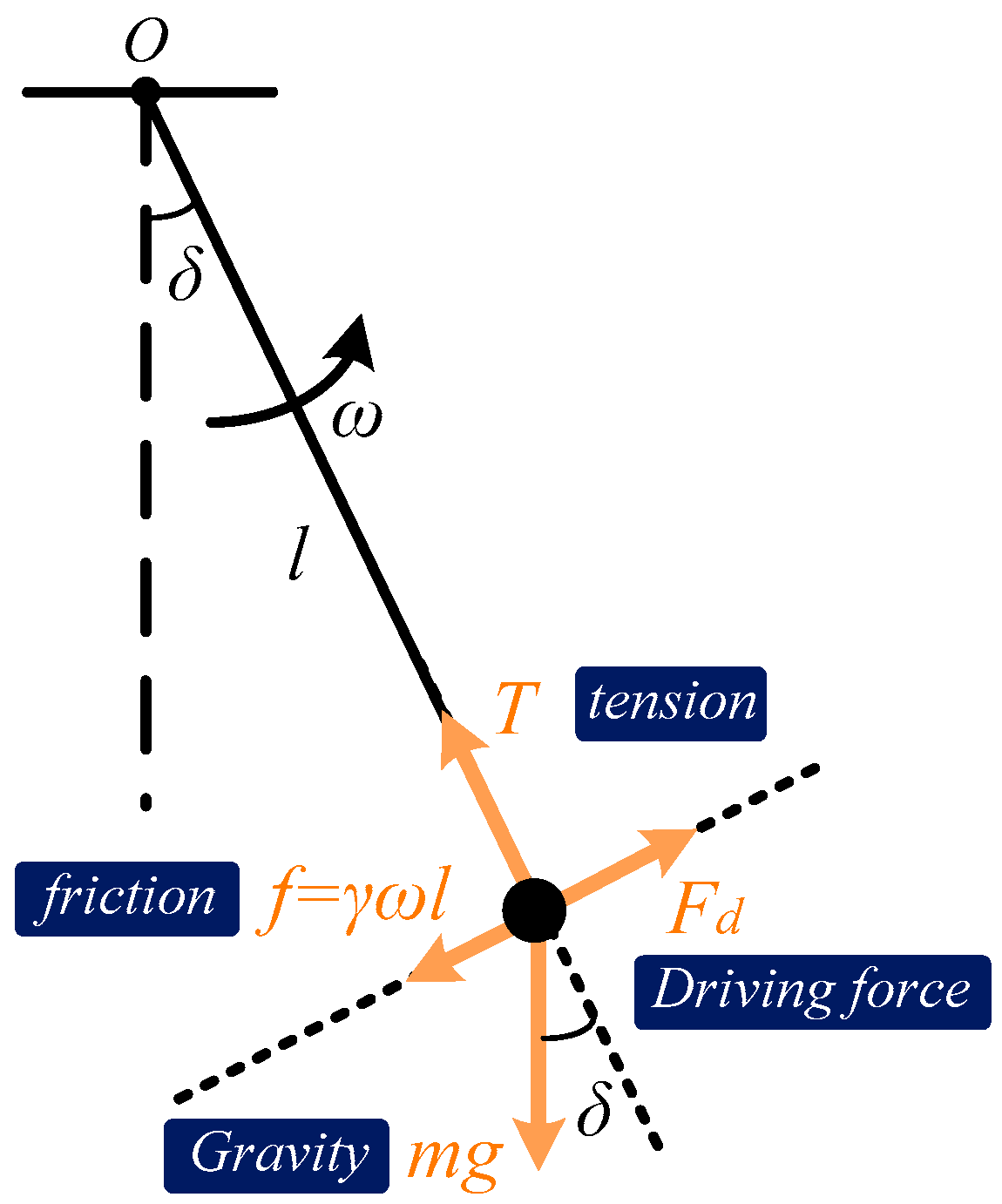
2.2. Modeling of a Simple Pendulum

Figure 2 shows the force analysis diagram of a pendulum [26], where l is the rope length, m is the mass of pendulum, δ is the pendulum angular position with respect to the vertical line, and ω represents the angular speed. Several different types of forces are applied on the pendulum, such as the gravity mg, the tension of the rope T, an external driving force Fd, and the air friction f. It is widely accepted that the friction f is proportional to the pendulum speed, i.e.,
f = γ v = γ ω l
where γ is the friction coefficient. Based on Newton’s second law, it can be obtained that
F d     γ ω l     m g   s i n   δ = m a
where a refers to the tangential acceleration speed. From (5), the angular acceleration speed can be calculated as
d 2 δ d t 2 = a l = F d m l     γ ω m     g l s i n   δ
Reorganizing (6) yields
d 2 δ d t 2 + γ m · d δ d t + g l s i n   δ = F d m l
which forms a generalized dynamic equation for describing the pendulum motion [26]. Comparing (3) and (7), it is interesting to find that the pendulum motion equation has the same format compared with that of the grid-connected VSG. This standard form can be expressed as
d 2 δ d t 2 + a 1 · d δ d t + a 0   s i n   δ = C
where a1, a0, and C are positive constants.

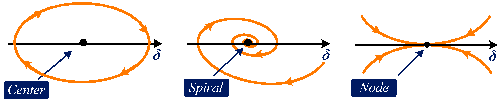
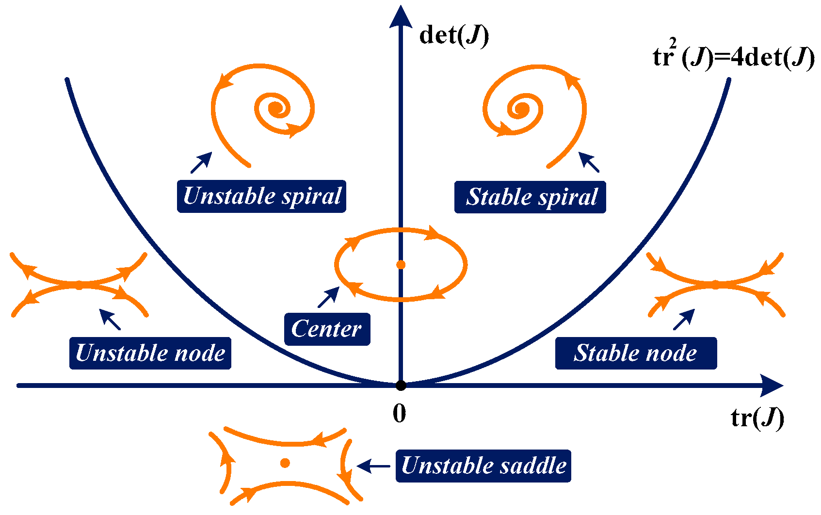
3. Preliminaries on Pendulum Phase Portrait

The above similarity on dynamic equation makes it possible to analyze the VSG transient stability through the analogy with a pendulum. Prior to this, some preliminary knowledge about pendulum phase portraits is provided in this section.
It has been quite a long time since physicists started to study the motion of a pendulum. Over the past centuries, a powerful analytical tool known as phase portrait analysis has been developed. The phase portrait is a geometric representation of pendulum motion trajectory, where the angular position δ is the horizontal coordinate and angular speed ω serves as the vertical coordinate. From a phase trajectory in the δ-ω plane, it is easy to predict whether the pendulum angular position will become stable or unstable (δ becomes unbounded).
Figure 3 shows typical phase portraits of a simple pendulum. With different system parameters and initial points, the corresponding phase trajectories are also completely different. For example, for the initial point A0, the angular speed ω is always positive in its forward path. Therefore, the pendulum is unstable since δ continuously increases and never reaches an equilibrium point. Similarly, the initial point A1 is also unstable, though its forward phase trajectory has marginally approached the δ-axis. In comparison, the corresponding phase trajectory of the initial point A2 will circulate around the equilibrium point E2. As a consequence, A2 is a stable initial point, according to the system stability definition.
It should be mentioned that the equilibrium point E2 in Figure 3 is one specific type of equilibrium point known as the center. In addition, a more generalized classification is shown in Figure 4, where the equilibrium points are classified as the center, the spiral, and the node. A center is an equilibrium point around which the phase portrait circulates rather than converges. It usually occurs when the pendulum has zero damping, i.e., γ = 0. A spiral is an equilibrium point occurring at the end of a phase trajectory. It indicates an insufficient damping effect and hence exhibits oscillatory behaviors in the neighborhood of the equilibrium point. Lastly, a node appears as the result of over-damping and makes sure that there is no oscillation in the phase portrait trajectory. Clearly, an initial point of the pendulum is stable if a center, a spiral, or a node exists in its forward phase portrait trajectory. Otherwise, the pendulum phase angle δ will become unbounded as time goes by.
In addition, an analytical tool can be used to judge whether an equilibrium point belongs to a center, a spiral, or a node. Without loss of generality, the standard form of (8) can be reorganized as
| d ω d t =   a 1 ·   ω     a 0   s i n     δ + C | d δ d t   = ω
Linearizing (9) at the equilibrium point, i.e., δ = δ0 and ω = 0, yields
d ω / d t d δ / d t =   J ·   ω δ = a 1 a 0   c o s   δ 0 1 0 ·   ω δ
where J is the Jacobin matrix, from which the characteristic equation is derived as
λ 2     t r ( J ) · λ + d e t ( J ) = 0
t r J =   a 1 ,   d e t J =   a 0 · c o s   δ 0
where tr(J) is the trace of the Jacobin matrix and det(J) refers to the determinant of the Jacobin matrix. The types of equilibria can be classified and related in the det-tr plane, as shown in Figure 5.
As can be seen from Figure 5, the entire det-tr plane is divided into several sub-regions. Among them, a stable region can be obtained if tr(J) > 0 and det(J) ≥ 0 are satisfied simultaneously. Moreover, the hyperbola tr2(J) = 4det(J) further determines the critical damping condition and distinguishes between the spiral and the node.

4. Transient Stability of a Grid-Connected VSG

The above knowledge is applied in this section to analyze the VSG transient stability. Discussions concern two different scenarios: without the damping effect and with the damping effect.

4.1. Transient Stability Without the Damping Effect

First, the scenario that a synchronous machine or a VSG has no damping effect is investigated. Considering that D = 0, the previously derived equation, i.e., (3), can be further simplified to characterize the VSG post-fault dynamic, i.e.,
d 2 δ d t 2 + 3 E V g I I 4 H X g I I · s i n   δ = P 0 2 H
where Vg-II and Xg-II are the post-fault grid voltage magnitude and line impedance, respectively. Additionally, the post-fault active power transmission limit PII is defined as
P I I = 3 E V g I I 2 X g I I
Combining (13) and (14),
d 2 δ d t 2 = 1 2 H ·   ( P 0     P I I s i n   δ )
Multiplying dt/ to both sides of (15) gives
d ω d t ·   d t d δ = d t d δ ·   [ P 0 2 H     P I I 2 H · s i n   δ ]
Rearranging (16) yields
ω ·   d ω   = ( P 0 2 H     P I I 2 H s i n   δ )   ·   d δ
The VSG phase portrait can be obtained by integrating both sides of (17):
0 ω ω ·   d ω = δ 0 δ ( P 0 2 H     P I I 2 H · s i n   δ ) ·   d δ
ω 2 =   f ( δ ) = P 0 H ·   ( δ     δ 0 )   + P I I H ( c o s   δ     c o s   δ 0 )
In (19), f (δ) is a mixed function made up of a linear function P0/H·δ, a trigonometric function PII/H·cos δ, and also a constant term determined by the initial condition. Figure 6 illustrates the typical post-fault VSG phase portraits. When the fault happens, the initial state immediately changes from point a to point b. Since P0 is larger than PII·sin δ between δ0 and δ1, the phase angle difference increases until point c is reached. Oppositely, a deceleration stage occurs between δ1 and δ2 because P0 is smaller than PII sin δ. From the phase portrait perspective, the VSG synchronization stability depends on whether the phase trajectory will cross the δ-axis before δ2. Figure 6a and Figure 6b show the stable and unstable scenarios, respectively. To ensure that the trajectory will cross the δ-axis before δ2, the condition below shall be satisfied:
f ( δ 2 ) < 0
From (19) and (20),
P 0   <   P I I ·   c o s   δ 2     c o s   δ 0 δ 2     δ 0
which gives the condition for maintaining the synchronization. To verify the correctness of the above phase portrait analysis, the stability condition is also derived through the conventional EAC, which defines the area Sabc in Figure 6 as the AA and Scod in Figure 6 as the DA. Their values are calculated as
S a b c = δ 0 δ 1 ( P 0     P I I s i n   δ )   ·   d δ =   P 0   ( δ 1     δ 0 ) +   P I I   ( c o s   δ 1 c o s   δ 0 )
S c o d = δ 1 δ 2 ( P I I s i n   δ     P 0 )   ·   d δ =   P 0 ( δ 1     δ 2 ) +   P I I   ( c o s   δ 1   c o s   δ 2 )
According to the EAC, the AA should be smaller than the DA such that a VSG, or a synchronous machine, is able to maintain the grid synchronization [17]. Therefore, it is required that
S a b c   S c o d =   P 0 ( δ 2     δ 0 ) +   P I I   ( c o s   δ 2     c o s   δ 0 )   <   0
A comparison indicates the same condition as (21) and validates the feasibility of the phase portrait analysis.
Notice that the damping effect of a synchronous machine is influenced by many factors, such as frictions and frequency-dependent loads in the system [17]. Owing to this reason, it is difficult to obtain the exact value of the damping effect, while assuming that D = 0 indicates the worst scenario. According to the EAC, if the AA is calculated to be larger than the DA, some efforts should be devoted to reverting the situation. Among them, one commonly adopted method is to clear the fault before the CCA. Yet, this strategy imposes requirements on the response speed of relaying and fault clearance.

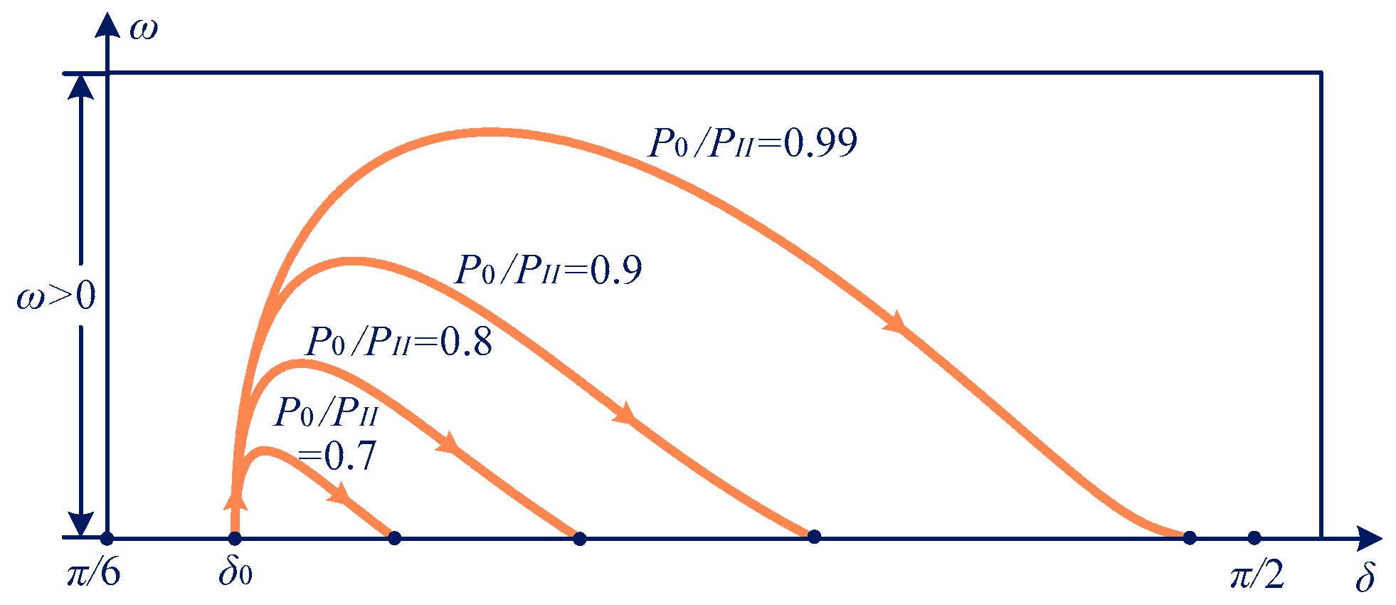
4.2. Transient Stability with the Damping Effect

The VSG damping coefficient D can be flexibly designed within a certain range, which helps to stabilize the VSG under large disturbances. In view of this, some questions arise inherently: Is it possible for a VSG to maintain grid synchronization even if the AA is larger than the DA? If so, how much damping is sufficient to reach this target? To properly answer these questions, analogical phase portrait analyses with damping effect are presented in this section. But before this, some clarifications are presented:
(1.) The scenarios where the AA is smaller than the DA are not considered, since the VSG synchronization stability can be easily guaranteed even without the damping effect.
(2.) It is assumed that there exists an equilibrium point after the fault. In other words, PII > P0. (It should be mentioned that the transient response without a post-fault equilibrium, i.e., PII < P0, will also be discussed later.)
The generalized phase portrait trajectories of (8) are plotted and illustrated in Figure 7, where the damping effect gradually increases from Figure 7a to f. δ0 is the initial phase angle difference and δ is the steady-state phase angle difference, if one ever exists. A comparatively small damping effect is applied in Figure 7a, and the corresponding trajectory (marked in a solid line) is compared with that without a damping effect (marked in a dashed line). It can be seen that the damping effect decreases the angular frequency difference ω and the nadir. This happens because the kinetic energy accumulated during the acceleration stage, which is proportional to ω2, is partially dissipated by the damping effect. Nevertheless, the system is still unstable as the phase portrait trajectory becomes unbounded and never crosses the δ-axis.
In Figure 7b, the increase in D, consequently, leads to more energy dissipations and helps to further decrease the nadir. A critical stability condition is met when D = Dcir1 and the nadir falls exactly on the δ-axis. Figure 7c depicts this scenario where the phase portrait trajectory reaches and then crosses the δ-axis. Due to the characteristics of a phase portrait, the crossing with the δ-axis is accomplished vertically with an infinite slope. Once ω becomes negative, the phase angle difference δ will decrease, even though the trajectory will not recover to the initial point δ0 due to the damping effect. Instead, it oscillates and finally converges to another value δ, indicating that the system is stable. According to the equilibrium point definition, the equilibrium point δ = δ and ω = 0 is a spiral.
Then, the damping effect keeps increasing and the oscillation around the equilibrium point becomes smaller, as shown in Figure 7d. When the damping effect is sufficiently large to reach the critical damping condition, i.e., D = Dcir2, the final equilibrium point in Figure 7e turns from a spiral to a node. As the damping effect becomes even stronger, the system is over-damped and free from oscillations, as shown in Figure 7f. In spite of this, the transient response becomes sluggish, accordingly.
The above phase portrait analysis indicates that it is possible to maintain synchronization when D > Dcir1. Nevertheless, it is not wise to select D as Dcir1 since the system will still suffer from serious oscillations. Alternatively, selecting D as Dcir2 provides superior performance in terms of system transient stability and oscillation damping. Recalling from the hyperbola in Figure 5, the value of Dcir2 can be calculated as
t r 2 ( J )     4   d e t ( J ) =   a 1 2     4 a 0 ·   c o s   δ = 0
From (3) and (8),
a 1 = D c i r 2 2 H ,   a 0 = 3 E V g I I 4 H X g I I
From (25) and (26),
D c i r 2 = 12 E · V g I I · H · c o s   δ X g I I 1 / 2
Moreover, it is important to make sure that the VSG transient stability is always guaranteed regardless of the initial and final states. Figure 8 depicts phase portrait trajectories with different final states (under the critical damping condition D = Dcir2). It is observed that the VSG transient stability can be ensured for various P0/PII ratios, even for the extreme condition that P0/PII is close to unity. This indicates that synchronization is easily maintained as long as an equilibrium point exists, i.e., P0/PII < 1.
For worse scenarios when the equilibrium does not exist, the VSG is not able to remain synchronized with the grid unless the fault has been cleared. If so, the initial phase angle difference at the recovery instant may vary according to the fault-clearing time. Figure 9 shows the phase portrait trajectories with different initial states. It was found that the trajectory always converges to the final state for any initial phase angle difference between −π and π. This attractive feature helps to release the stress of fault clearance. (Note that the conventional EAC requires fault to be cleared before the CCA; otherwise, synchronization will be lost.)

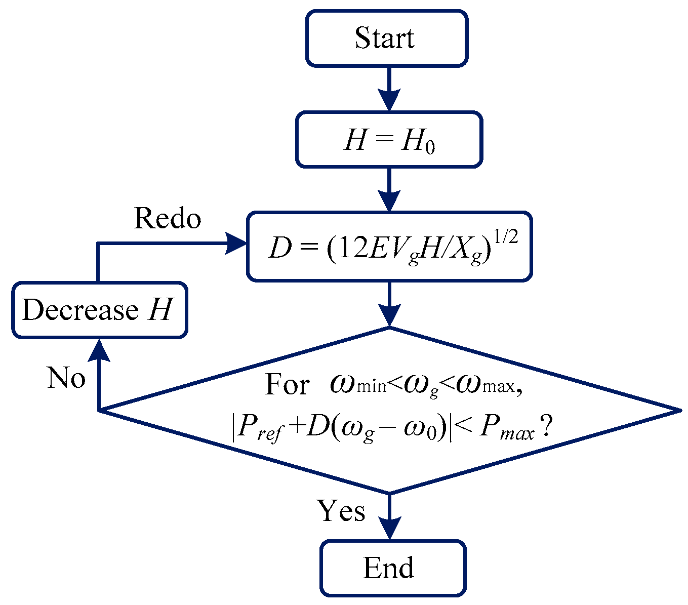
4.3. Parameter Design Procedure

Based on the above analyses, a parameter design procedure is also provided to properly tune the VSG inertia coefficient H and the damping coefficient D. In order to guarantee the critical damping condition for various post-fault conditions, the value of D is determined as
D   =       12 E V g H X g 1 / 2   >   12 E · V g I I · H · c o s   δ X g I I 1 / 2
Figure 10 shows a simple flowchart for control parameter design. To start, the inertia coefficient is tuned as an initial value H0, which is the maximum inertia support that can be provided by the converter and the DC-side energy storage unit. Next, the damping coefficient D is tuned according to (28). Though the critical damping condition has been satisfied, the grid code also requires that the steady-state VSG active power P0 = Pref + D(ω0ωg) cannot exceed its capacity limit Pmax when grid frequency ωg varies between ωmin and ωmax [8]. If this requirement is not satisfied, the value of H is decreased and a new damping coefficient value is calculated. This process will be repeated until the power capacity limit condition is satisfied.

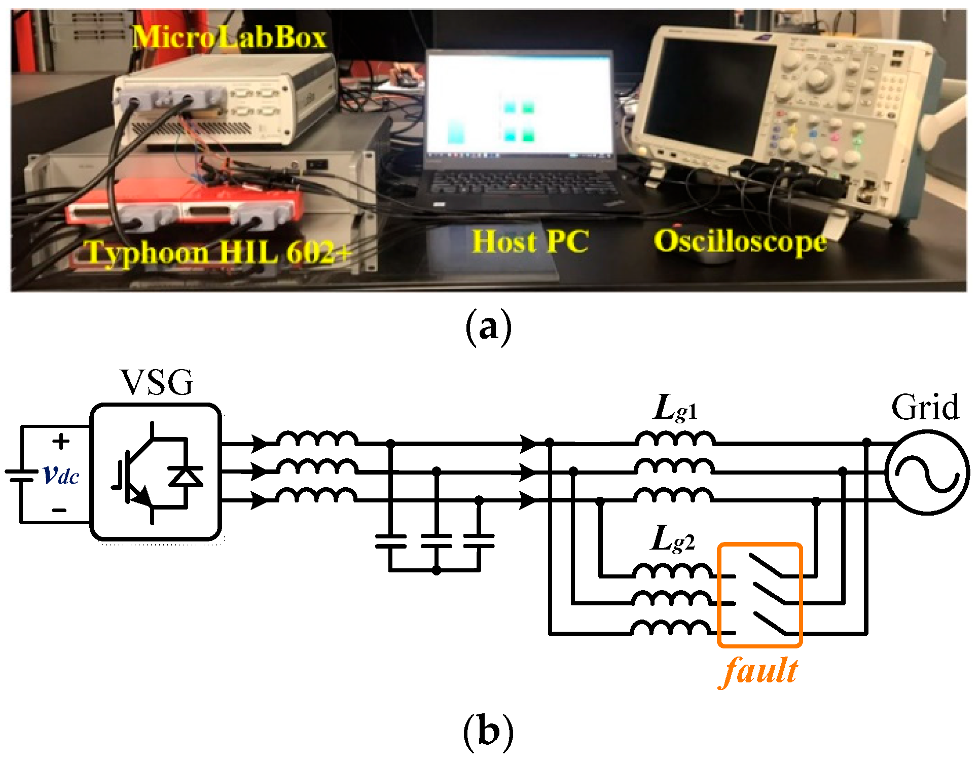
5. Hardware-in-Loop Simulation Results

In order to validate the aforementioned theoretical findings, a grid-connected VSG was built under Typhoon HIL 602 and the digital controls were implemented by a dSPACE MicroLabBox. Figure 11a shows the laboratory setup and Figure 11b shows the fault scenario, where an open-circuit fault happens and cuts off one power transmission line. The key system parameters are provided in Table 1. Two different situations have been studied, and the corresponding results are shown below.

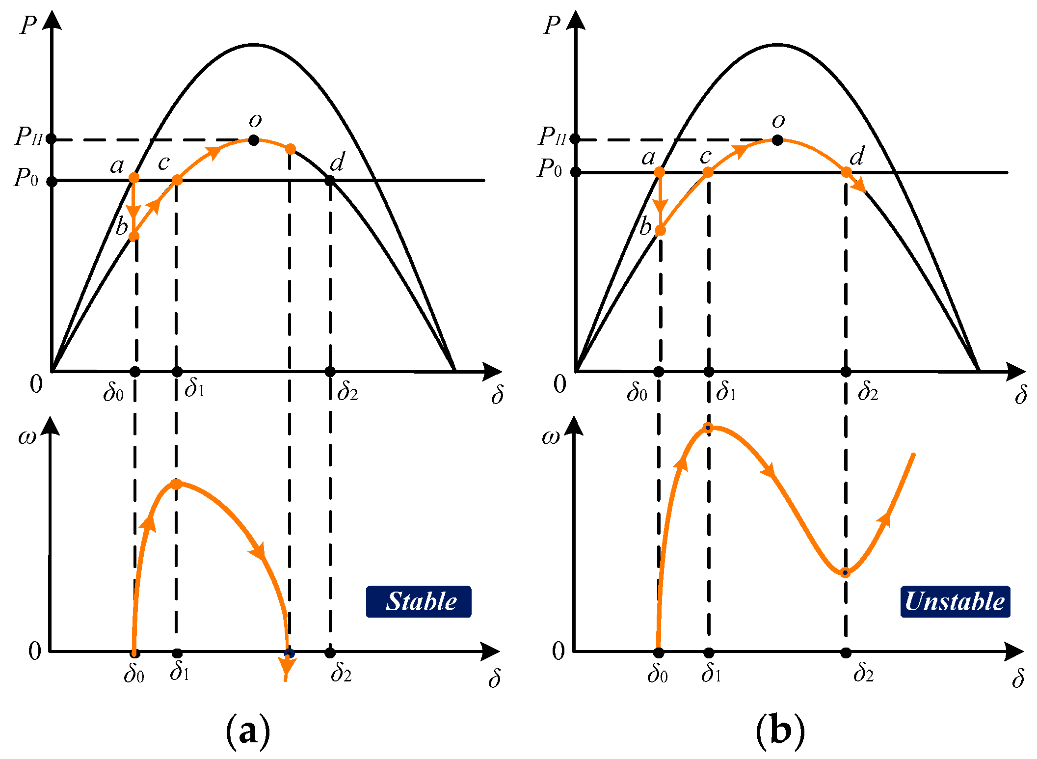
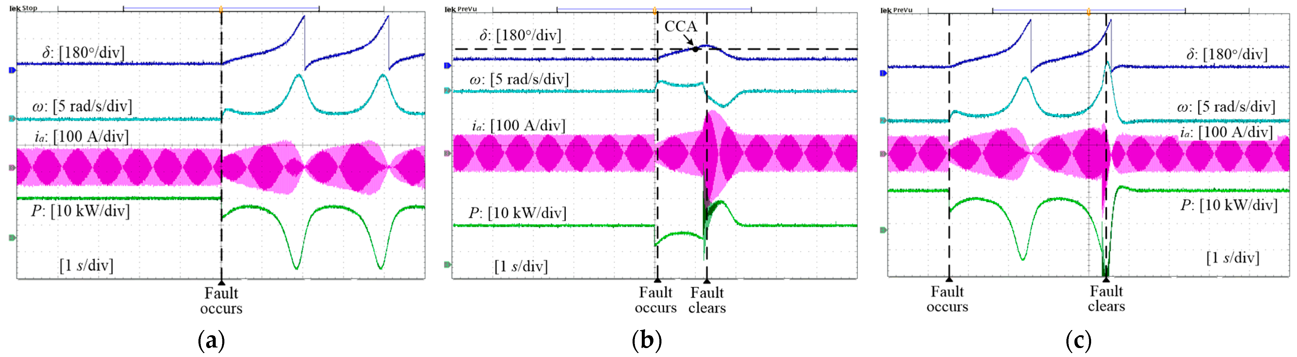
5.1. VSG Responses with Post-Fault Equilibrium

Figure 12 shows VSG dynamic responses with different steady-state power P0 values. In Figure 12a, P0 equals 5 kW. The associated AA and DA are calculated as 282 rad·W and 9611 rad·W, respectively. As the DA is much larger than the AA, the VSG grid synchronization is easily guaranteed and δ smoothly increases from 12.4° to 25.4°. In Figure 12b, P0 equals 10 kW. According to the EAC, the VSG will be out of step because the DA (1088 rad·W) is smaller than the AA (1356 rad·W). However, it can be seen that the VSG transient stability is still well guaranteed. A similar result is also observed in Figure 12c, where P0 = 11.5 kW is very close to the power transfer limit PII. Though the DA (29.5 rad·W) is significantly smaller than the AA (1990 rad·W), δ finally converges to its equilibrium value 84.2° without losing synchronization. From the above results, it is clear that VSG synchronization stability can be easily guaranteed as long as an equilibrium exists after the fault.

5.2. VSG Responses Without Post-Fault Equilibrium

For some worse scenarios where post-fault equilibrium does not exist, the VSG transient stability was tested, as shown in Figure 13. In Figure 13a, no recovery is achieved after the fault occurs. Since P0 = 15 kW already exceeds the active power transfer limit PII, by no means can a VSG maintain the grid synchronization. Hence, the VSG becomes out of step after the fault. As a result, the phase angle difference δ, the angular speed difference ω, and the delivered active power P oscillate periodically. In Figure 13b, the fault is cleared after the CCA. According to the conventional EAC, the synchronization cannot be maintained. Yet, it can be seen that the VSG is able to resynchronize with the grid after the fault clearance. An even worse situation test is shown in Figure 13c, where the fault clearance is very slow and the VSG has gone through several rounds of oscillation. Nonetheless, the VSG resynchronization ability is not affected, as clearly seen in Figure 13c. The testing results are in good accordance with the previously presented phase portrait analysis.

6. Conclusions

This paper studies the transient stability of the grid-connected VSG through analogical phase portraits. It is revealed that with the proper tuning of the damping coefficient, the synchronization can always be maintained as long as an equilibrium point exists. Additionally, for severe faults scenarios where there is no equilibrium point, the VSG can still resynchronize with the grid after clearing the fault. This resynchronization ability is found to be independent of the fault-clearing time and therefore releases the system post-fault operation stress. The above theoretical findings are then verified by both phase portrait trajectories and HIL simulation results.

Author Contributions

Conceptualization, S.W.; Methodology, S.W.; Software, J.W.; Validation, J.W.; Formal analysis, Y.Q.; Writing—original draft, H.Z. and Y.Q.; Writing—review & editing, H.Z. All authors have read and agreed to the published version of the manuscript.

Funding

This research received no external funding.

Data Availability Statement

The original contributions presented in the study are included in the article, further inquiries can be directed to the corresponding author.

Conflicts of Interest

Authors Si Wu and Jun Wu were employed by the company China LongYuan Power Group Cooperation Limited. The remaining authors declare that the research was conducted in the absence of any commercial or financial relationships that could be construed as a potential conflict of interest.

References

  1. Fang, J.; Li, H.; Tang, Y.; Blaabjerg, F. On the Inertia of Future More-Electronics Power Systems. IEEE J. Emerg. Sel. Top. Power Electron. 2019, 7, 2130–2146. [Google Scholar] [CrossRef]
  2. Huang, Y.; Wang, Y.; Li, C.; Zhao, H.; Wu, Q. Physics Insight of the Inertia of Power Systems and Methods to Provide Inertial Response. CSEE J. Power Energy Syst. 2022, 8, 559–568. [Google Scholar]
  3. Hatziargyriou, N.; Milanovic, J.; Rahmann, C.; Ajjarapu, V.; Canizares, C.; Erlich, I.; Hill, D.; Hiskens, I.; Kamwa, I.; Pal, B.; et al. Definition and classification of power system stability—Revisited & extended. IEEE Trans. Power Syst. 2021, 36, 3271–3281. [Google Scholar] [CrossRef]
  4. Rathnayake, D.B.; Razzaghi, R.; Bahrani, B. Generalized Virtual Synchronous Generator Control Design for Renewable Power Systems. IEEE Trans. Sustain. Energy 2022, 13, 1021–1036. [Google Scholar] [CrossRef]
  5. Driesen, J.; Visscher, K. Virtual Synchronous Generators. In Proceedings of the IEEE PES General Meeting, Pittsburgh, PA, USA, 20–24 July 2008; pp. 1–3. [Google Scholar]
  6. Liu, J.; Hou, Y.; Guo, J.; Liu, X.; Liu, J. A Cost-Efficient Virtual Synchronous Generator System Based on Coordinated Photovoltaic and Supercapacitor. IEEE Trans. Power Electron. 2023, 38, 16219–16229. [Google Scholar] [CrossRef]
  7. Li, C.; Yang, Y.; Cao, Y.; Wang, L.; Dragicevic, T.; Blaabjerg, F. Frequency and Voltage Stability Analysis of Grid-Forming Virtual Synchronous Generator Attached to Weak Grid. IEEE J. Emerg. Sel. Top. Power Electron. 2022, 10, 2662–2671. [Google Scholar] [CrossRef]
  8. Meng, X.; Liu, J.; Liu, Z. A Generalized Droop Control for Grid-Supporting Inverter Based on Comparison Between Traditional Droop Control and Virtual Synchronous Generator Control. IEEE Trans. Power Electron. 2019, 34, 5416–5438. [Google Scholar] [CrossRef]
  9. Wu, H.; Ruan, X.; Yang, D.; Chen, X.; Zhao, W.; Lv, Z.; Zhong, Q.-C. Small-Signal Modeling and Parameters Design for Virtual Synchronous Generators. IEEE Trans. Ind. Electron. 2016, 63, 4292–4303. [Google Scholar] [CrossRef]
  10. Roldan-Perez, J.; Rodriguez-Cabero, A.; Prodanovic, M. Design and Analysis of Virtual Synchronous Machines in Inductive and Resistive Weak Grids. IEEE Trans. Energy Convers. 2019, 34, 1818–1828. [Google Scholar] [CrossRef]
  11. Chen, J.; Donnell, T. Parameter Constraints for Virtual Synchronous Generator Considering Stability. IEEE Trans. Power Syst. 2019, 34, 2479–2481. [Google Scholar] [CrossRef]
  12. Huang, L.; Xin, H.; Wang, Z. Damping Low-Frequency Oscillations Through VSC-HVdc Stations Operated as Virtual Synchronous Machines. IEEE Trans. Power Electron. 2019, 34, 5803–5818. [Google Scholar] [CrossRef]
  13. Hirase, Y.; Sugimoto, K.; Sakimoto, K.; Ise, T. Analysis of Resonance in Microgrids and Effects of System Frequency Stabilization Using a Virtual Synchronous Generator. IEEE J. Emerg. Sel. Top. Power Electron. 2016, 4, 1287–1298. [Google Scholar] [CrossRef]
  14. Ambia, M.N.; Meng, K.; Xiao, W.; Al-Durra, A.; Dong, Z.Y. Interactive Grid Synchronization-Based Virtual Synchronous Generator Control Scheme on Weak Grid Integration. IEEE Trans. Smart Grid 2022, 13, 4057–4071. [Google Scholar] [CrossRef]
  15. Huang, L.; Xin, H.; Yang, H.; Wang, Z.; Xie, H. Interconnecting Very Weak AC Systems by Multiterminal VSC-HVDC Links with a Unified Virtual Synchronous Control. IEEE J. Emerg. Sel. Top. Power Electron. 2018, 6, 1041–1053. [Google Scholar] [CrossRef]
  16. Khajehoddin, S.A.; Karimi-Ghartemani, M.; Ebrahimi, M. Grid-Supporting Inverters with Improved Dynamics. IEEE Trans. Ind. Electron. 2019, 66, 3655–3667. [Google Scholar] [CrossRef]
  17. Tang, C.K.; Graham, C.E.; El-Kady, M.; Alden, R.T.H. Transient stability index from conventional time domain simulation. IEEE Trans. Power Syst. 1994, 9, 1524–1530. [Google Scholar] [CrossRef]
  18. Kundur, P. Power System Stability and Control; McGraw-Hill: New York, NY, USA, 1994. [Google Scholar]
  19. Yorino, N.; Priyadi, A.; Kakui, H.; Takeshita, M. A New Method for Obtaining Critical Clearing Time for Transient Stability. IEEE Trans. Power Syst. 2010, 25, 1620–1626. [Google Scholar] [CrossRef]
  20. Hou, X.; Sun, Y.; Zhang, X.; Lu, J.; Wang, P.; Guerrero, J.M. Improvement of Frequency Regulation in VSG-Based AC Microgrid Via Adaptive Virtual Inertia. IEEE Trans. Power Electron. 2020, 35, 1589–1602. [Google Scholar] [CrossRef]
  21. Li, D.; Zhu, Q.; Lin, S.; Bian, X.Y. A Self-Adaptive Inertia and Damping Combination Control of VSG to Support Frequency Stability. IEEE Trans. Energy Convers. 2017, 32, 397–398. [Google Scholar] [CrossRef]
  22. Chang, G.W.; Nguyen, K.T. A New Adaptive Inertia-Based Virtual Synchronous Generator with Even Inverter Output Power Sharing in Islanded Microgrid. IEEE Trans. Ind. Electron. 2024, 71, 10693–10703. [Google Scholar] [CrossRef]
  23. Xue, Y.; Van Custem, T.; Ribbens-Pavella, M. Extended equal area criterion justifications, generalizations, applications. IEEE Trans. Power Syst. 1989, 4, 44–52. [Google Scholar] [CrossRef]
  24. Li, R.; Yan, X.; Wang, Y.; Zhang, Q.; Chen, Z. Improved Transient Modeling and Stability Analysis for Grid-Following Wind Turbine: Third-Order Sequence Mapping EAC. IEEE Trans. Power Deliv. 2024, 39, 2015–2027. [Google Scholar] [CrossRef]
  25. Tang, Y.; Tian, Z.; Zha, X.; Li, X.; Huang, M.; Sun, J. An Improved Equal Area Criterion for Transient Stability Analysis of Converter-Based Microgrid Considering Nonlinear Damping Effect. IEEE Trans. Power Electron. 2022, 37, 11272–11284. [Google Scholar] [CrossRef]
  26. Paudyal, S.; Ramakrishna, G.; Sachdev, M.S. Application of Equal Area Criterion Conditions in the Time Domain for Out-of-Step Protection. IEEE Trans. Power Deliv. 2010, 25, 600–609. [Google Scholar] [CrossRef]
  27. Tedrake, R. Underactuated Robotics: Learning, Planning, and Control for Efficient and Agile Machines; Massachusetts Institute of Technology: Cambridge, MA, USA, 2019. [Google Scholar]
  28. Wu, H.; Wang, X. Design-Oriented Transient Stability Analysis of Grid-Connected Converters with Power Synchronization Control. IEEE Trans. Ind. Electron. 2019, 66, 6473–6482. [Google Scholar] [CrossRef]
  29. Wu, J.; Ren, S.; Zhu, M.; Wang, Z.; Wang, R.; Qi, Y. Transient Stability Analysis of Virtual Synchronous Machine Considering the Damping Effect. In Proceedings of the 2024 IEEE 7th International Electrical and Energy Conference (CIEEC), Harbin, China, 10–12 May 2024; pp. 2653–2658. [Google Scholar]
  30. Li, Y.; Liu, J.; Liu, Y.; Yang, S.; Du, Z. Transient stability analysis of virtual synchronous generator with current saturation by multiple Lyapunov functions method. IET Gener. Transm. Distrib. 2024, 18, 1014–1025. [Google Scholar] [CrossRef]
  31. Shuai, Z.; Shen, C.; Liu, X.; Li, Z.; Shen, Z.J. Transient Angle Stability of Virtual Synchronous Generators Using Lyapunov’s Direct Method. IEEE Trans. Smart Grid 2019, 10, 4648–4661. [Google Scholar] [CrossRef]
  32. Qi, Y.; Deng, H.; Fang, J.; Tang, Y. Synchronization Stability Analysis of Grid-Forming Inverter: A Black Box Methodology. IEEE Trans. Ind. Electron. 2022, 69, 13069–13078. [Google Scholar] [CrossRef]
Figure 1. Control block diagram of a grid-connected VSG [32]. (a) Circuit and control block diagram; (b) equivalent diagram of active power loop.
Energies 18 03495 g001
Figure 2. Force analysis diagram of a simple pendulum.
Energies 18 03495 g002
Figure 3. Typical phase portraits of a simple pendulum (without damping effect).
Energies 18 03495 g003
Figure 4. Classifications of the equilibrium points.
Energies 18 03495 g004
Figure 5. Diagram indicating the classification of equilibrium points in the det-tr plane.
Energies 18 03495 g005
Figure 6. VSG phase portraits after a large system disturbance: (a) stable scenario; (b) unstable scenario.
Energies 18 03495 g006
Figure 7. Analogical phase portrait trajectories with a gradually increasing damping coefficient D. (a) D is much smaller than Dcri1. (b) D is close to Dcri1. (c) D equals to Dcri1. (d) D is between Dcri1 and Dcri2. (e) D equals to Dcri2. (f) D is greater than Dcri2.
Energies 18 03495 g007
Figure 8. Phase portrait trajectories with different final states.
Energies 18 03495 g008
Figure 9. Phase portrait trajectories with different initial states.
Energies 18 03495 g009
Figure 10. A simple flow chart for control parameter design.
Energies 18 03495 g010
Figure 11. HIL simulation platform: (a) photo of laboratory setup; (b) illustration of the fault scenario.
Energies 18 03495 g011
Figure 12. VSG dynamic responses when the post-fault equilibrium exists. (a) P0 = 5kW, the EAC is satisfied; (b) P0 = 10kW, the EAC is not satisfied; (c) P0 = 11.5kW, the EAC is not satisfied.
Energies 18 03495 g012
Figure 13. VSG dynamic responses when the post-fault equilibrium does not exist, P0 = 15 kW. (a) Fault not cleared; (b) fault cleared after the CCA; and (c) fault cleared after being out of step.
Energies 18 03495 g013
Table 1. Key system parameters.
ParametersDescriptionsValues
Vg, E0Nominal voltage magnitude155 V
ω0Nominal grid frequency50 Hz
HVSG inertia coefficient100
DVSG damping coefficient3050 s·W
PrefVSG nominal power at ω02 kW
Lg1, Lg2Line impedances20 mH
PIIPost-fault active power limit11.56 kW
Disclaimer/Publisher’s Note: The statements, opinions and data contained in all publications are solely those of the individual author(s) and contributor(s) and not of MDPI and/or the editor(s). MDPI and/or the editor(s) disclaim responsibility for any injury to people or property resulting from any ideas, methods, instructions or products referred to in the content.

