Abstract
With the rapid development of artificial intelligence technology, DRL has shown great potential in solving complex real-time optimal power flow problems of modern power systems. Nevertheless, traditional DRL methodologies confront dual bottlenecks: (a) suboptimal coordination between exploratory behavior policies and experience-based data exploitation in practical applications, compounded by (b) users’ distrust from the opacity of model decision mechanics. To address these, a model–data hybrid-driven physics-informed reinforcement learning (PIRL) algorithm is proposed in this paper. Specifically, the proposed methodology uses the proximal policy optimization (PPO) algorithm as the agent’s foundational framework and constructs a PI-actor network embedded with prior model knowledge derived from power flow sensitivity into the agent’s actor network via the PINN method, which achieves dual optimization objectives: (a) enhanced environmental perceptibility to improve experience utilization efficiency via gradient-awareness from model knowledge during actor network updates, and (b) improved user trustworthiness through mathematically constrained action gradient information derived from explicit model knowledge, ensuring actor updates adhere to safety boundaries. The simulation and validation results show that the PIRL algorithm outperforms the baseline PPO algorithm in terms of training stability, exploration efficiency, economy, and security.
1. Introduction
OPF has become one of the most fundamental issues in power system operation planning and electricity market transactions, aiming at improving economy while ensuring the safe and stable operation of power systems. In recent years, the problems of energy shortage and environmental pollution have become more and more prominent, which has driven the rapid development of renewable energy source technology [1], and many renewable energy sources are deployed and connected to the power system. With the continuous integration and modification of high-proportion renewable energy sources and multi-type load demand, profound changes in the power system are led by significantly different operating characteristics from the traditional synchronous generator, as follows.
- (1)
- Distributed renewable energy sources exhibit pronounced stochastic, intermittent, and fluctuating characteristics, leading to a continuous increase in operational uncertainty in the new power system. This results in frequent node voltage fluctuations and flicker and rapidly shifting power flow [2], which constrain the space for safe and stable operation in the new power system, thereby endangering its overall stability.
- (2)
- The increasing integration of controllable power electronic equipment and higher interruptible load access ratios has made the operation and dispatch of the modern power system more flexible, thereby heightening the complexity of power system optimization [3].
This poses a significant challenge to the OPF strategy of the power system. On the one hand, the high uncertainty in the modern power system triggers frequent changes in voltage and power flow, compelling dispatch strategies to reduce dispatch time intervals to improve economic efficiency and safety, which intensifies real-time computation requirements for OPF. Consequently, traditional high-computation-cost optimization methods are becoming increasingly inadequate for modern power systems. Additionally, the number of state and control variables in the OPF model is inevitably increased by the extensive integration of electronic power equipment and controllable loads, introducing additional constraints, highlighting nonlinear, nonconvex characteristics and making it challenging to obtain the global optimal solution to this OPF problem [4].
Many scholars have conducted extensive research on the challenges and issues of the modern power system OPF. Among the model-based optimization methods, the objective function is first formulated based on the system output–cost relationship, with the output of each unit and load shedding defined as control variables and corresponding state constraints imposed [5]. Depending on the solution method, model-based methods are generally classified into two main categories. The first category introduces convex relaxation of the exact AC power flow constraints to enable the application of numerical algorithms, such as Newton’s method [6] and the interior-point method [7]. In [8], the QC relaxation method was introduced with an improved linear convex envelope, which to some extent reduced the distance between the optimization results and the optimal solution, but there were still a few cases where the optimization results deteriorated. In [9], a nested decomposition method was proposed for multi-level networks, which improved the convergence and computational efficiency by using lower-level convex optimization problems based on the nested and recursive framework. In [10,11], the second-order cone programming model and semidefinite programming model are used for relaxation, improving the convergence of the iterative numerical algorithm to some extent. However, the primary shortcoming of the above model-based optimization algorithms is that the accuracy of the relaxed model is insufficient, making it challenging to ensure the precision of solution results. To address this issue, the second category of search algorithm methods with primitive non-convex models has been applied and rapidly developed to find the optimal solution by performing global or local searches in the feasible domain for the safe operation of the modern power system. In [12], a non-dominated sorting genetic algorithm is applied to multi-objective OPF problems involving wind and solar energy. In [13], the jellyfish algorithm is applied to OPF problems involving power markets and renewable energy sources. Both algorithms improve computational efficiency to some extent. In [14], the cuckoo optimization algorithm is used to further improve the computational efficiency and enhance the convergence of the algorithm. However, these algorithms suffer from drawbacks such as parameter sensitivity and a tendency to fall into local optima. Furthermore, the algorithm performance is coupled with the initial value and highly depends on the fitness of the model in OPF problems, resulting in poor generalizability and extensibility, making it difficult to ensure their optimization capability. Overall, the traditional model-based OPF algorithm often struggles to balance computational efficiency and accuracy in power system scheduling scenarios and cannot effectively cope with the challenges of modern power systems.
With the development of artificial intelligence, the DRL, one of the new generation of artificial intelligence technologies, can rapidly make response decisions based on the observed state due to its model-free nature and rapid function approximation capabilities of neural networks [15]. In recent years, it has made significant progress in the field of power systems, particularly in solving OPF. Reference [16] proposed a Bayesian neural network-based OPF method that considers the spatial–temporal probabilities of multi-source renewable energy. Reference [17] introduced the TD3-based multi-agent reinforcement learning method for optimal generation control in DC microgrids, accelerating convergence through distributed reinforcement learning. Reference [18] further introduced a hierarchical learning method for DRL agents, achieving highly efficient energy management. However, as a model-free approach, DRL algorithms lack environmental perception in the early stages of training, requiring extensive exploration time to perceive the environment. This results in high computational costs and time demands when training suitable models for high-dimensional OPF problems. Furthermore, the learning process relies to some extent on the abstract environmental advantage estimates provided by the critic network. In complex environments, the critic network is more prone to estimation errors, which can misguide the agent’s learning updates, leading to sudden performance degradation and the generation of substantial amounts of ineffective or suboptimal experience.
PINNs, a significant branch of interpretable deep learning (DL), offer effective guidance for training neural networks by embedding a priori physics knowledge as regularization terms in the network’s loss function. This approach significantly accelerates the training speed and credibility of neural networks while providing innovative solutions to the inherent limitations of data-driven methods mentioned previously. References [19,20] proposed PINN methods applied to AC-OPF and DC-OPF, respectively, that can rapidly project optimization results. Reference [21] proposed the SINDy algorithm to further address the efficiency issues of PINN algorithms, significantly reducing network training time in grid parameter estimation problems. Reference [22] leveraged a PINN to address the challenges of strong nonlinearities in low-inertia systems, successfully applying it to nonlinear system identification for power system dynamics and achieving significantly superior estimation performance to that of the unscented Kalman filter. However, PINNs still fall within the domain of DL and its extensions; therefore, their application at the OPF level still possesses common, inherent drawbacks, as follows.
- (1)
- As a supervised learning paradigm, DL relies on high-quality, large-scale labeled datasets for support, and the trained models are typically limited to addressing the specific system represented by the training dataset. This makes DL poorly suited to adapting to the rapidly evolving operational conditions and structures of modern power systems.
- (2)
- Power system dispatch optimization is a multi-timestep decision-making process constrained by unit ramp-rate limits. DL methods struggle to produce accurate multi-timestep decision trajectories when solving dispatch strategies, rendering them impractical for direct application and significantly limiting their generalizability.
Inspired by the philosophy of physics-informed methods, PIRL has emerged as a new branch of reinforcement learning. By combining environmental perception and knowledge-guided techniques with DRL, PIRL demonstrates immense potential due to its low computational cost, high scalability, and a learning capability distinct from PINNs.
Several approaches have explored enhancing the agent’s perception. The PIDTRL algorithm, proposed in [23], adds a physics-informed layer to the agent, providing it with the ability to perceive the DAB inductor current. Similarly, Reference [24] proposed using the admittance matrix to construct a PIRL algorithm that enhances the agent’s ability to perceive power flow changes. Reference [25] improves training convergence by encoding prior knowledge into images using the solution space diagram method. However, these PIRL methods that enhance environmental perception require additional or indirect use of data-driven techniques, and the stability of this perception capability can introduce potential issues to the training process.
Other studies have focused on constraining the agent’s actions to avoiding invalid actions. Reference [26] introduced physics-informed exploration into a safe reinforcement learning algorithm, using a model-based method to confine the agent’s actions to a safe region and reduce exploration of invalid actions. Reference [27] proposed using an action masking technique based on power flow sensitivity to block actions that are predicted to cause limit violations. However, this method of action masking does not directly guide the actions themselves, resulting in relatively limited improvements in training speed and computation cost. Furthermore, it can restrict the agent’s exploration of certain extreme environmental conditions, making it difficult to quantify the impact on the agent’s optimality. The preceding analysis highlights a critical research gap: the need for a PIRL framework that can directly utilize model knowledge to efficiently guide the agent’s learning process, thereby enhancing training efficiency, reducing computational cost, and improving final policy quality. To fill this gap, a model–data hybrid-driven PIRL approach is proposed in this paper to provide an RT-OPF strategy that combines low training costs with generalizability. The proposed approach uses PPO as the agent blueprint and constructs a PI-actor network with an independent model perception mechanism based on power flow model sensitivity with the PINN method. The significant contributions of this paper are as follows.
- (1)
- After the mathematical model of the RT-OPF problem is systematically formulated, a Markov decision process (MDP) model is developed based on this optimization problem, incorporating unit ramping constraints. Safety and economic efficiency are modeled as reward functions to support the agent’s training process, enabling the acquisition of gradient information that combines safety and economic performance.
- (2)
- Based on power flow sensitivity, the influence relationship between agent actions and system states is established, serving as the prior model knowledge essential for guiding the agent. Then, building on the PINN method, the PI-actor network is introduced after an action constraint violation degree index, incorporating safety gradient information, and utilized as a regularization term for model knowledge. This actor network leverages the action–system state loop for backpropagation to derive gradients of safety information, thereby providing critical model guidance during the network update process.
- (3)
- An RT-OPF solution framework based on a model–data hybrid-driven PIRL approach is established. Compared to classical data-driven methods, the proposed approach builds upon the PPO algorithm by embedding a PI-actor network, leveraging both model knowledge and data-driven techniques to compute safety-economic gradient information for training the agent. The proposed method demonstrates significant advantages in terms of safety and economic performance in RT-OPF. Furthermore, the integration of black-box models with white-box knowledge substantially enhances the trustworthiness of the actor network.
The paper is organized as follows. In Section 2, we provide the OPF problem of the dispatch model, and the detailed MDP model is established based on it. In Section 3, as the baseline, the PPO algorithm is formulated for application to the OPF problem, and the proposed PIRL algorithm is illustrated. In Section 4, the performance of the proposed PIRL algorithm is compared with PPO and IPS in the IEEE 39-bus system. Conclusions and future work are presented in Section 5.
2. Preliminaries
2.1. RT-OPF Problem Description
Before establishing the MDP model of RT-OPF, the mathematical description of the RT-OPF problem, which is the formulation basis of MDP, is presented as follows.
2.1.1. Objective Function
The RT-OPF problem is formulated as a quadratic programming problem focused on the economic optimization of generating unit outputs, and the objective function aimed at minimizing operation cost is represented as follows:
where represents the unit active power output, and are the unit cost curve coefficients, and denotes the set of generation units. It should be noted that in this paper, to maximize renewable energy integration, the renewable energy sources are modeled as deterministic active and reactive power injections at the PQ bus. Therefore, the objective function solely focuses on the economic optimization of the thermal power units’ generation.
2.1.2. Constraints
The model’s constraints include power system operational constraints, as well as generation unit output and ramp rate constraints. Each constraint is defined as follows.
- (a)
- Node power balance constraints:where represents the unit reactive power output and and indicate the active power and reactive power consumption in the node and represent the conductance and susceptance between the and nodes. The set of nodes in the system is denoted by .
- (b)
- Node voltage security constraints:where and indicate the lower and upper limits of the node’s voltage, while represents the node’s voltage.
- (c)
- Unit generation constraints:where the active and reactive power output limit of the unit are denoted by , , , and , respectively.
- (d)
- Ramp rate limits:where and denote the generation ramp-up limit and ramp-down limit of the unit.
2.2. MDP Modeling of RT-OPF Problem
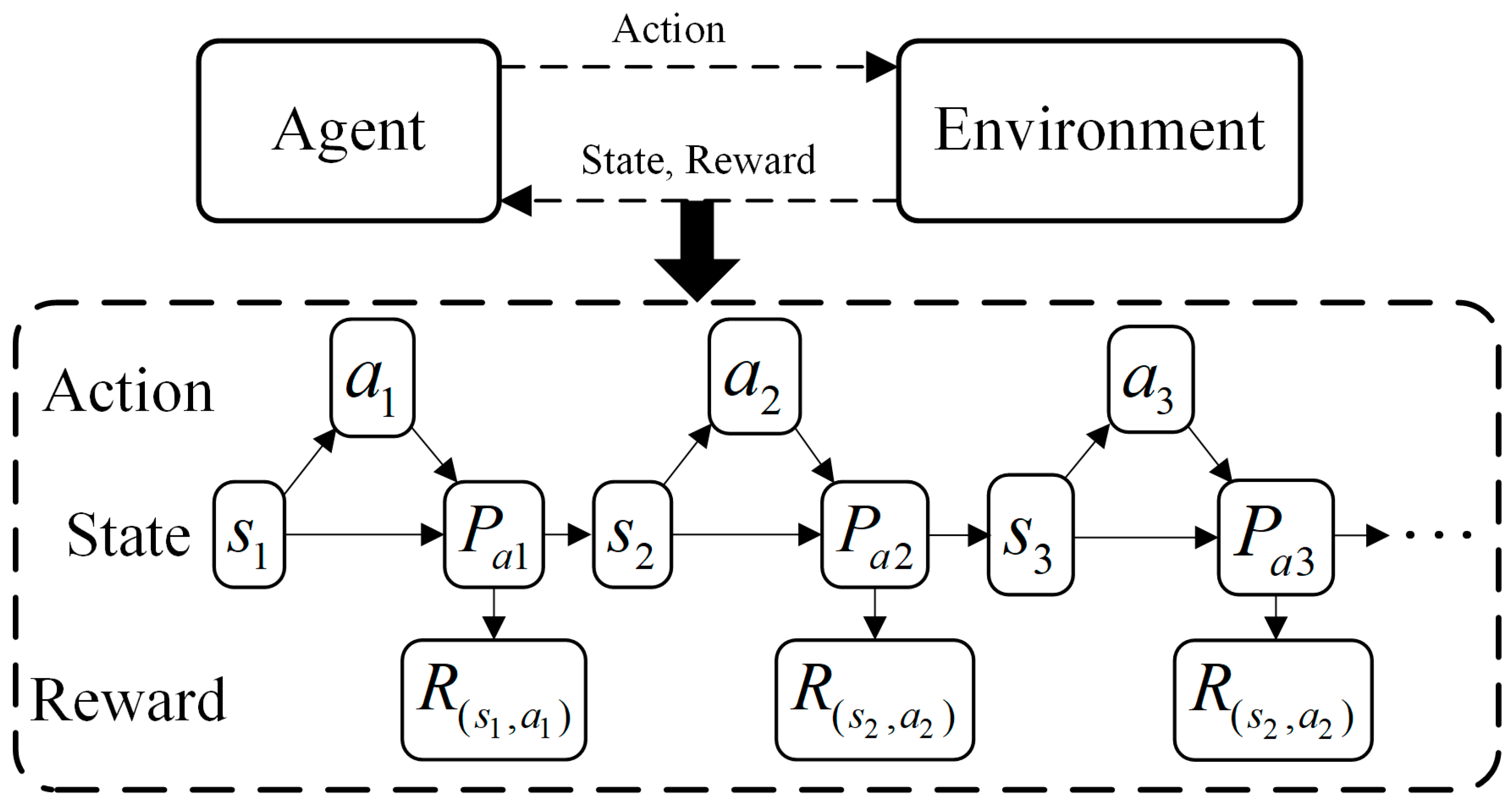
Based on the mathematical formulation of the RT-OPF problem, an MDP model is constructed to describe the interaction process in DRL, as illustrated in Figure 1. The proposed MDP architecture comprises two interactive components—the environment and the agent—whose sequential engagement is modeled as a Markov chain governed by state–action–transition–reward quadruples .
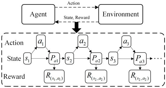
Figure 1.
Brief MDP architecture.
The , which means a state set containing important feature information of power system dispatch, is established as:
The state contains of five pieces of information: the voltage and load demand of each node, active and reactive output of units and , and renewable energy source output .
The action set , the dispatch action taken in response to observing the state containing the network information, is presented as:
Note that to consider the unit ramping constraints during the dispatch operation and ensure the validity of the cumulative reward in the MDP, all actions are designed as adjustment values rather than target values, with unit ramping constraints serving as the upper and lower bounds. The actions include the adjustment values of active power outputs for all nodes except the slack bus, as well as the voltage adjustments of units at PV buses and the reactive power output adjustments of renewable energy sources at PQ buses.
According to (8) and (9), the Markov state transition probability can be obtained as:
In the RT-OPF problem, the dispatch center formulates plans based on forecasts of load and renewable energy source outputs. It is generally assumed that the accuracy of these forecasts is sufficient to support effective dispatch operation planning. Therefore, the Markov state transition process can be considered a deterministic process, which can be defined as:
Therefore, quadruples are transformed to .
denotes the corresponding reward generated by the transition of the power flow state of the environment from to after the execution of action generated by reinforcement learning agent. Thus, the reward directly reflects the merit of the state after the transition occurs, i.e., the economy and safety of the power flow adjustment. In this paper, to make the DRL agent learn safer and more economical strategies, according to (1)–(7), a reward function based on the AC-OPF model is designed as follows:
where , , and are penalization coefficients, which are usually negative. denotes the subtask ensuring the security, and , , and represent Boolean values that determine whether actions are exceeded.
3. Proposed Algorithm
In this section, as the baseline algorithm, the classic PPO is deployed to solve the AC-OPF problem. Subsequently, the proposed PIRL algorithm integrating PPO and model knowledge derived from power flow sensitivity is presented.
3.1. Baseline PPO Algorithm
PPO is an improved on-policy optimization algorithm that is based on the actor–critic framework with the core idea of finding the optimal policy to maximize the cumulative reward through state advantage. Therefore, utilizing the previously constructed Markov process, the intelligent agent’s policy constructed by the actor network of PPO is as follows:
where denotes normal distribution, whose mean and standard deviation are indicated by the actor network output and , respectively. indicates the parameters of the network influencing the output.
To maximize the cumulative reward , the actor network loss is formulated as follows:
where represents the deviation of the action probability distribution between the old and new policies. To mitigate the risk of excessively large network parameter updates that could hinder the convergence of the policy, the clipping parameter is introduced to limit the influence of deviations on the loss function. is the advantage function, which judges whether is better than , and is calculated according to the generalized advantage estimation (GAE) method:
where and are the hyperparameters denoting discount coefficient and priority discount coefficient, respectively. is a value function, which is represented by the critic network with parameters to estimate the value of state . Thus, to approximating the true state value function by incrementally updating the estimate, the critic network loss can be defined as follows:
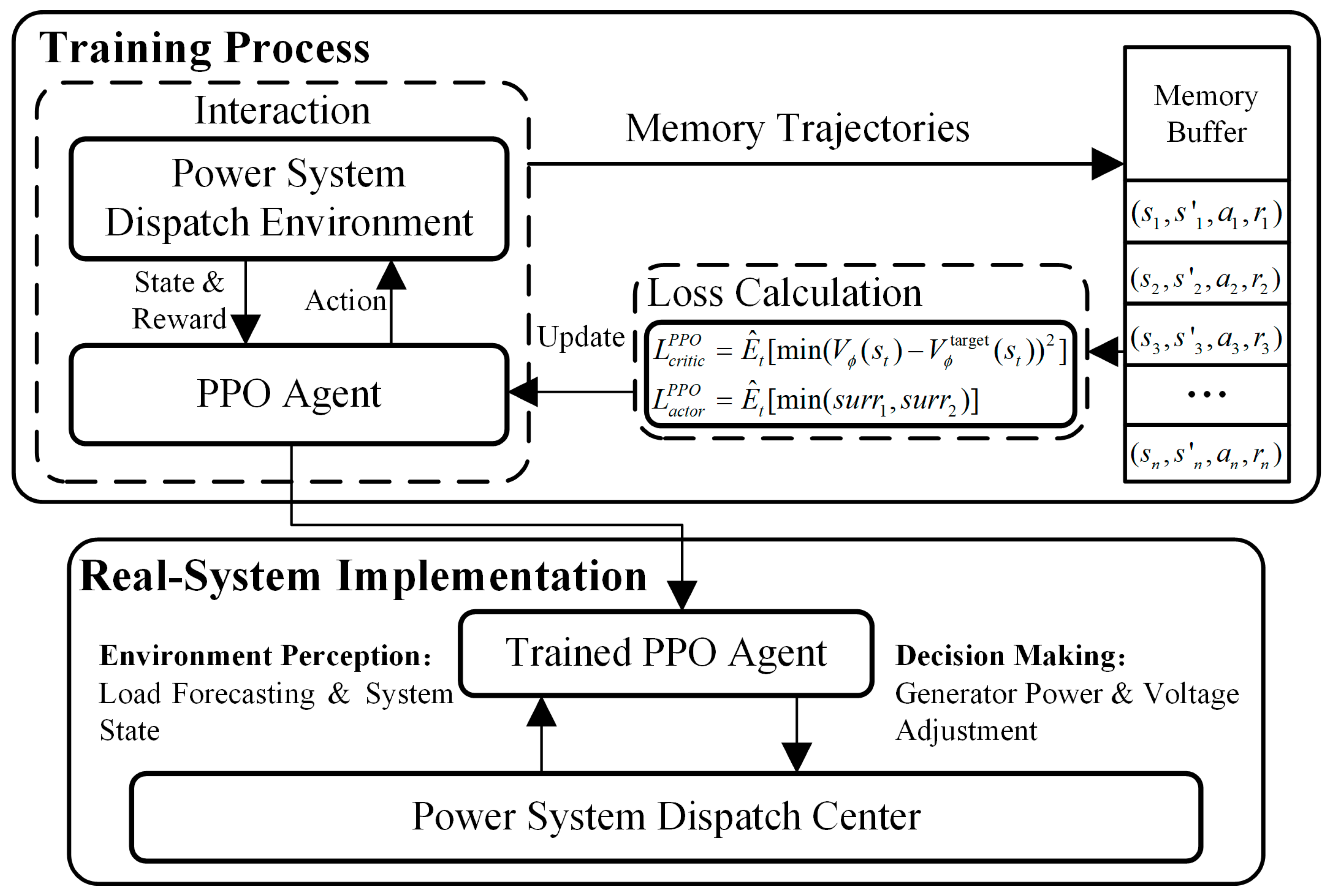
The proposed baseline PPO algorithm framework to solve the AC-OPF problem is illustrated in Figure 2.
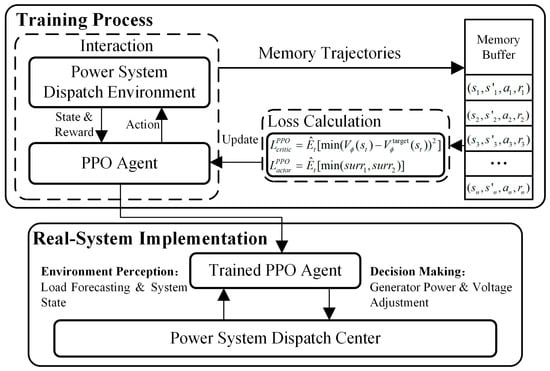
Figure 2.
PPO framework for power system dispatch.
Firstly, the PPO agent interacts with the power system dispatch simulation environment to collect experience trajectories. Then, based on (18) and (21), trajectories are utilized to calculate the PPO loss function and each network’s parameter gradient. The actor network and critic network parameter updating formulas, respectively, are expressed as follows:
where and denote the learning rate of the actor network and critic network, respectively. After being fully trained, the agent can be deployed in the real system and provide actions to achieve near-optimal power flow based on observed state.
3.2. Proposed PIRL Algorithm
According to the mentioned PPO algorithm framework, the PPO algorithm estimates the state advantage value relied on the data-driven critic network. References [28,29] indicate that excessive variance in value estimation by the critic network can lead to deviations between the safety-economic gradient information and the state advantage, resulting in erroneous iterations and ineffective exploration in the actor network, significantly impairing the learning and convergence performance of the agent. This issue is particularly pronounced in high-dimensional action–state spaces, where large value estimation variances are more likely to occur.
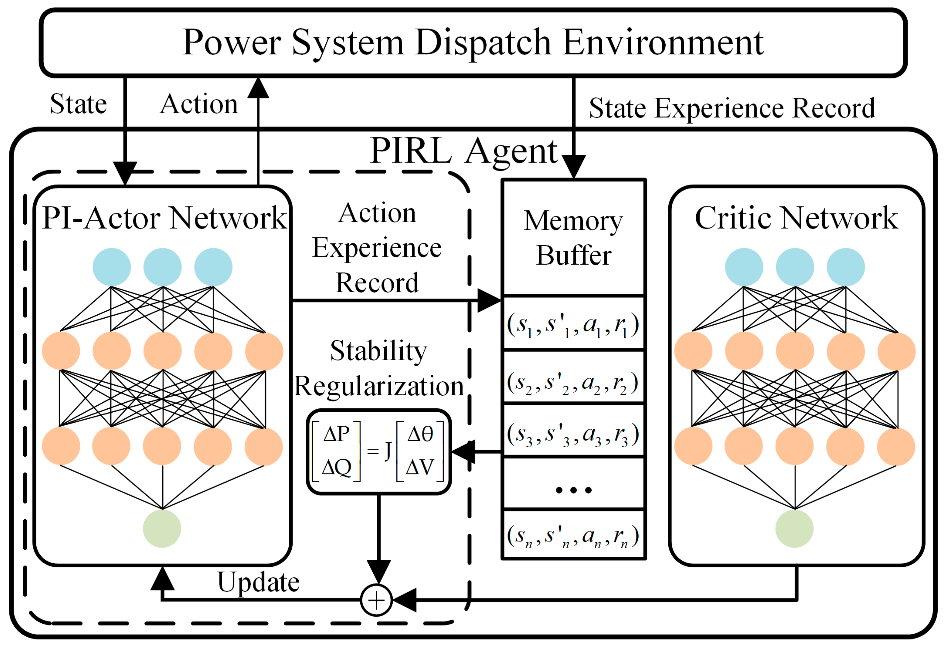
Therefore, the PIRL algorithm proposed in this paper leverages the PI-actor network to directly compute safety-economic gradient information from prior model knowledge, explicitly guiding the update direction of the actor network, as shown in Figure 3.
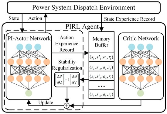
Figure 3.
Architecture of proposed PIRL.
In this algorithm, the data-driven component operates identically to that of PPO. First, the critic network estimates the value of each state within experience trajectories. Subsequently, the GAE method is used to calculate state-advantage values. Based on the magnitude of these values, the probability of the corresponding action is iteratively increased or decreased.
The model-driven component decoupled from the data-driven part does not rely on a neural network. Instead, it first leverages power flow sensitivity to predict the change in the power flow state corresponding to an action, thereby establishing a feedback path. This predicted value and feedback path are then used to construct a regularization term that is embedded into the loss function.
We firstly consider the linearized representation of the Newton–Raphson correction equation at the system’s stable point:
Based on Equation (9), this equation can be reformulated as follows:
where the Jacobian inverse matrix reflects the sensitivity of active and reactive power injections to phase angles and voltages at each bus. Combined with Equation (11), a linear prediction equation for the action and the prediction of system state can be further established:
Based on Equations (28) and (29), the change in power flow and the resulting predicted state corresponding to each action can be calculated. Then, to provide the agent with a model-driven mechanism for perceiving the feasibility of its actions, a stability regularization term based on the action–system state loop is proposed:
where and represent the upper and lower bounds of the system state, determined based on the inequality constraints (4)–(7). Obviously, this regularization term exhibits two key characterizations: (a) when the system satisfies all inequality constraints, the gradient of the regularization term is zero, while the system violates these constraints and the regularization term yields a gradient directed toward the system’s stability boundary with magnitude of 1, thus consistently reflecting the safety information of the action; (b) the gradient computation does not rely on the black-box neural network model, but is instead derived through system sensitivity calculations, ensuring clear interpretability and trustworthiness.
Through the PINN method, the PI-actor network and the PIRL algorithm are further proposed using this regularization term. The loss function of PI-actor network can be expressed as follows:
where represents the regularization term weight coefficient, with a larger value enhancing the guidance of the actor network’s update direction. The proposed PIRL algorithm is detailed in Algorithm 1.
The introduction of the PI-actor network, with its explicit, purely model-driven update mechanism, endows our PIRL framework with three significant advantages, as follows.
- (1)
- Direct Guidance and Efficiency: The framework formulates a model-driven regularization term from a power flow sensitivity-based feedback loop. This term provides direct, physics-based guidance to the agent’s learning process at every step, which significantly accelerates training and reduces overall computational costs.
- (2)
- Enhanced Robustness and Stability: The model-driven and data-driven components are decoupled. This architecture prevents the deterministic physics-based guidance from being destabilized by the stochastic nature of the data-driven exploration, resulting in a more robust and stable training phase with less sensitivity to hyperparameters.
- (3)
- Modularity and Extensibility: The decoupled design is inherently modular. The physics-informed component can be adapted or replaced to suit different physical systems or constraints without requiring a complete redesign of the core DRL agent. This simplifies deployment and enhances the algorithm’s extensibility.
The establishment of the PI-actor network provides the PIRL agent with an additional environment perception mechanism based on prior model knowledge, significantly improving the agent’s experience utilization rate, learning efficiency, and convergence performance.
| Algorithm 1 PIRL training process |
| Initial PIRL agent, memory buffer |
| for in episode |
| Initial power system simulator environment |
| Reset memory buffer |
| for time in 24 × 2 |
| for in step times |
| Agent’s actor network selects action based on state |
| Environment returns the reward and the next state |
| Memory buffer records |
| Break if power flow not converges |
| end for |
| end for |
| for in epochs |
| extract total experiences samples from Memory Buffer |
| utilizing experiences samples to calculate loss by: |
| backpropagate loss value to compute the network gradients based on loss value, update PIRL agent network by: |
| end for |
| end for |
| return PIRL model |
4. Case Study
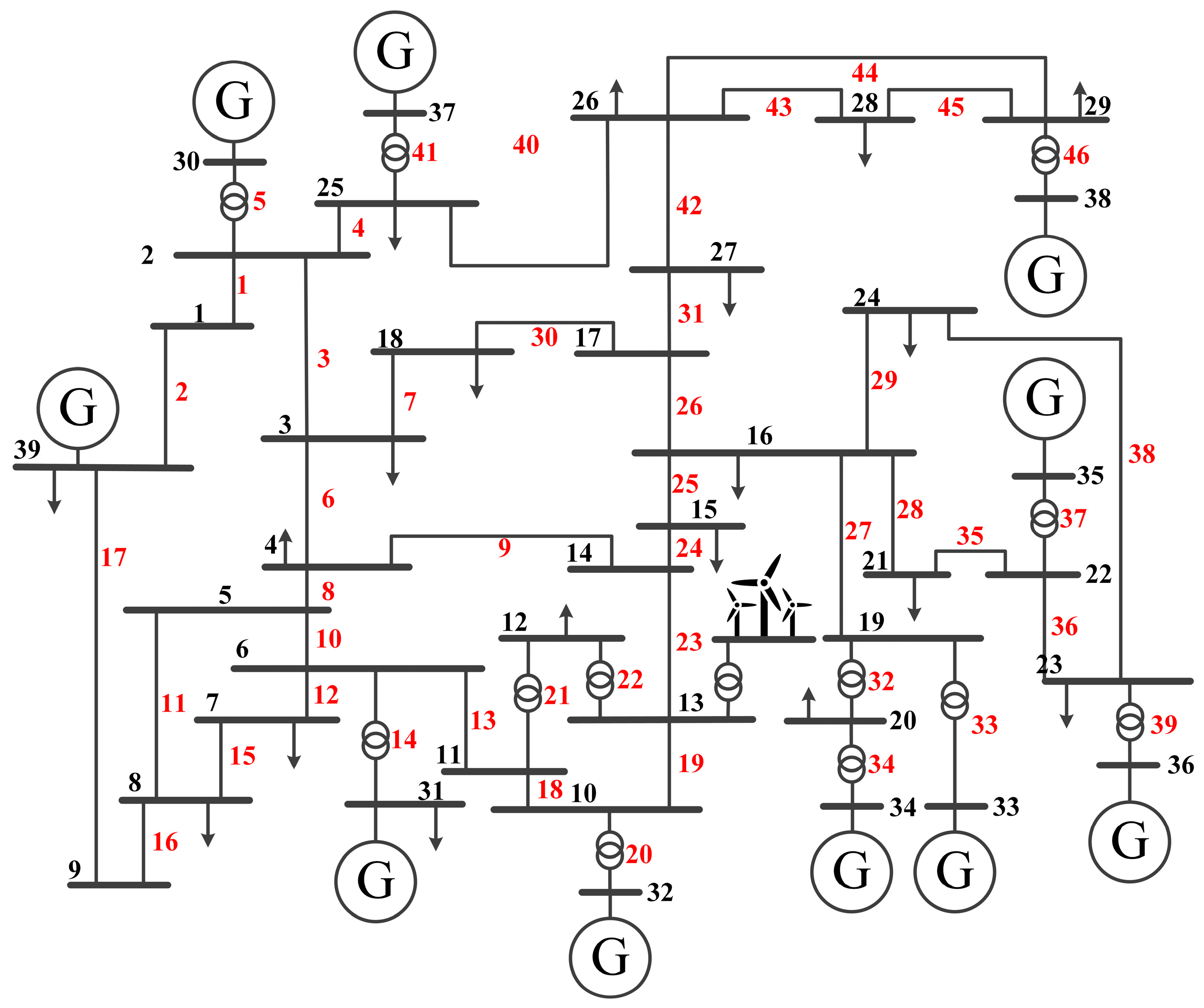
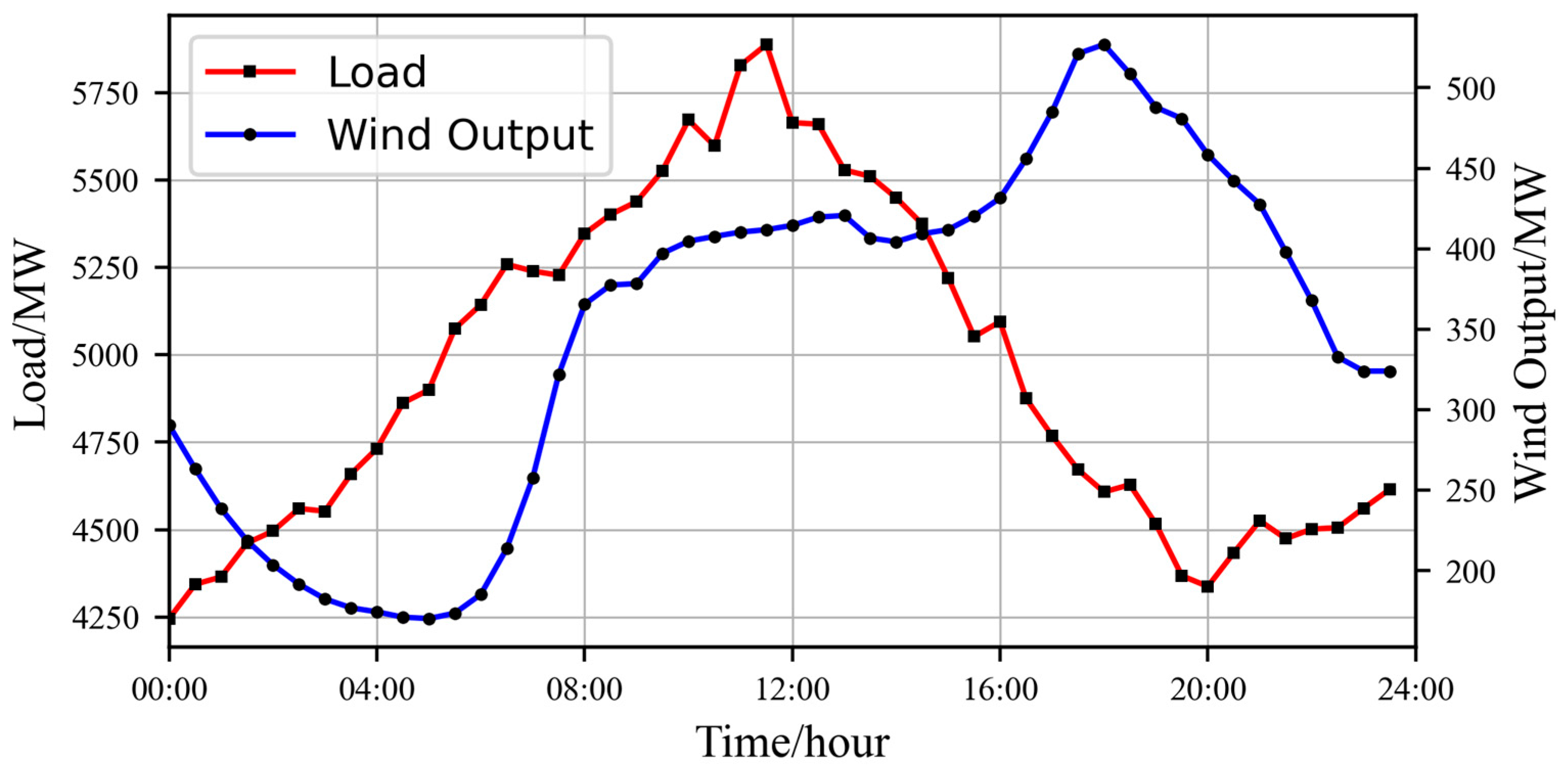
The effectiveness of the proposed PIRL is tested in the IEEE 39-bus system case shown in Figure 4, which includes 39 buses, 10 thermal generator units, 19 loads, and 46 lines. The total load curve is depicted in Figure 5. It is necessary to note that a wind farm, whose 24 h curve is also shown in Figure 5, is connected with bus 13 in this paper. When formulating the dispatch plan, it is assumed that the forecast data is accurate. Therefore, based on a 30 min dispatch interval, 48 evenly spaced data points are selected from both the load curve and the wind farm output curve to represent the forecasted load and wind farm generation at each dispatch time. The case study is based on Python (v3.11.9) language, using the PaddlePaddle (v3.0.0b1) framework to implement the PIRL algorithm, and the simulation platform is MATPOWER (v8.0), which is a tool for power system optimization in MATLAB (v2023b). The experiments were performed on a computer equipped with 17–12,700 k 3.2 GHz CPU (Intel, Santa Clara, CA, USA) and an Nvidia RTX A4000 GPU (Nvidia, Santa Clara, CA, USA).
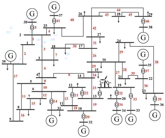
Figure 4.
Topology illustration of IEEE 39-bus system.
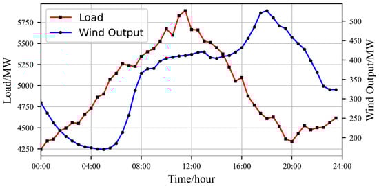
Figure 5.
Data curve of load and wind farm output.
4.1. Algorithm and Environment Settings
In terms of network setting, considering a large or wide network in DRL algorithm will lead to overfitting and poor generalization. Based on the state and action space dimensions being 155 and 18 respectively, two six-layer neural networks are set up for the actor network and the critic network. In the critic network, the layers are configured with [155, 2048, 1024, 256, 32, 1] neurons, respectively. This architecture consists of an input layer with 155 neurons, hidden layers with [2048, 1024, 256, 32] neurons, an output layer with 1 neuron, and the activation function using the ReLU function. Similarly, we set up [155, 2048, 1024, 256, 32, 18] neurons in the actor network layer.
In addition, we first selected reference points for both the PIRL and PPO hyperparameters by adopting typical, well-established values from foundational DRL studies [30,31]. These reference values are widely recognized for providing a robust baseline for a wide range of optimization tasks. For the hyperparameters unique to PIRL, we tuned them by monitoring the reward function curves and instances of system limit exceedance during training. Finally, the hyperparameters of the PIRL and PPO algorithms were selected, which are shown in Table 1.

Table 1.
Hyperparameter and environment parameter selection.
In the environment setup, we mainly focus on the selection of the parameters of the reward function, which determines whether the environment is effective. Reference [32] points out that if the death penalty is better than the maximum possible cumulative reward for survival, the agent is likely to prefer terminating the episode prematurely during the training process. Therefore, we introduce the death penalty selection formula in this paper:
where represents the empirical parameter. Given that the survival reward does not remain at its minimum value for extended periods, is typically set between 10% and 30% in accordance with the environmental conditions. In this paper, is set to 30%. Therefore, the parameters of the reward function (12) are identified and also shown in Table 1.
4.2. Comparison in the Training Process
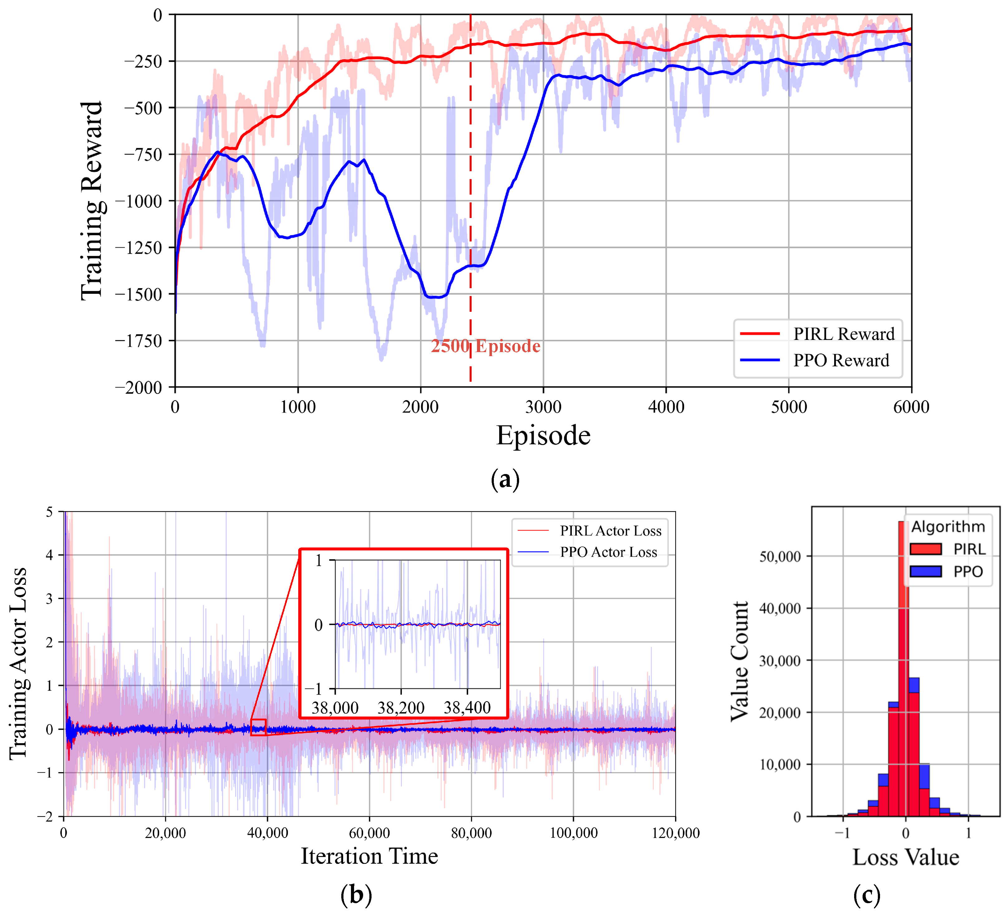
To enable the agent to comprehensively perceive environmental dynamics and adapt to diverse operational scenarios, a substantial number of offline scenarios and considerable training time are required. Accordingly, we formulate the total system load as stochastically allocated across individual load nodes, generating 6000 unique daily dispatch scenarios. The agent explores these scenarios by formulating dispatch decisions for each scenario and collects experiential knowledge for iterative learning. The total training time to complete the 6000 episodes was 13.32 h for the PIRL algorithm and 12.72 h for the PPO algorithm, respectively. A comparative analysis of the learning processes between the two algorithms is illustrated in Figure 6.
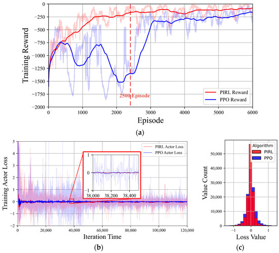
Figure 6.
Training process under difference two DRL methods: (a) training reward curves; (b) loss curves of actor networks; (c) distribution statistical histogram of actor loss value.
(a) During initial training phases, the PPO algorithm required approximately 2500 episodes to progressively comprehend environmental characteristics. Prior to this threshold, the episode total rewards exhibit significant fluctuations ranging between −1800 and −500, with no evident improvement trend observed. Benefiting from PPO’s robustness and environmental comprehension capabilities, subsequent to the initial exploration, the agent rapidly identifies optimal decision-making trajectories and converges swiftly toward near-optimal solutions. In contrast, the PIRL algorithm leverages the PINN method to guide its actor exploration, achieving rapid convergence toward optimal strategies during initial training phases while substantially reducing episodes required for environmental understanding.
(b) and (c) The actor iteration loss curves and statistical histograms of loss values demonstrate that both algorithms achieve convergence within reasonable bounds. However, the PIRL algorithm, whose actor network benefits from the physical knowledge guidance, exhibits superior stability with a more compact and concentrated loss value distribution compared to PPO throughout most training iterations.
4.3. Comparison of Optimality and Security
In this section, to verify the optimality of the proposed PIRL algorithm, we first define the optimality gap metric:
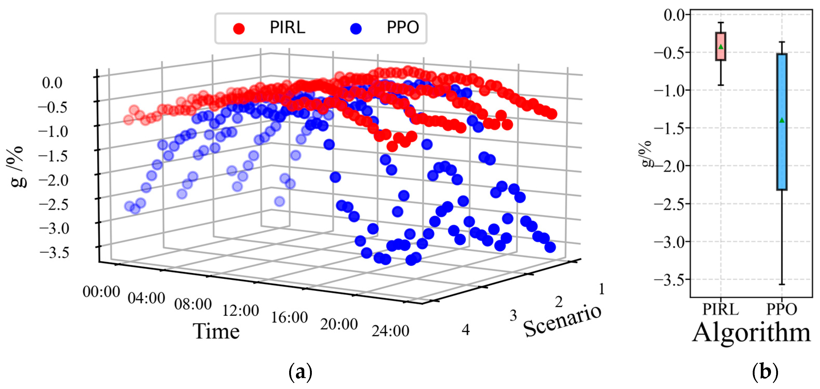
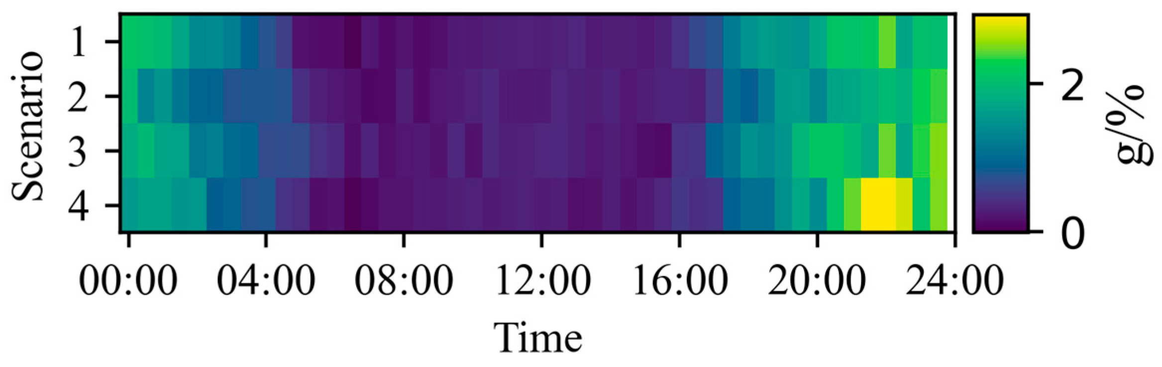
where the cost of algorithm optimization results is represented by , while the referent value denotes the solution of the interior point solver (IPS). The metric is employed to quantify the solution deviation of DRL relative to the IPS, where a lower value indicates higher divergence from optimality. To systematically evaluate the proposed PIRL algorithm, four test scenarios are selected from the 6000-day dispatch scenarios. Subsequently, MATPOWER IPS was utilized to compute optimal solutions for 4 × 48 = 192 s data points, which serve as benchmark references for comparative performance analysis. The PIRL algorithm and the baseline PPO algorithm are evaluated across the 4-day dispatch scenarios, and the optimality gap metric of each algorithm is systematically computed and compared in all scenarios. As demonstrated in Figure 7, the trained PIRL and PPO algorithms maintained within 4% across all four operational scenarios. However, the PPO algorithm exhibited higher exceeding 2% during the 0:00–5:00 and 16:00–24:00 periods, whereas the PIRL algorithm consistently constrained below 1% throughout all periods and scenarios. Box-plot analysis demonstrates that PIRL achieves significantly lower mean value (indicated by green triangle in plot) with a tighter distribution. To rigorously evaluate the algorithmic superiority between PIRL and PPO, the superiority deviation metric was systematically quantified and is shown in Figure 8. The results demonstrate that PIRL consistently exhibits positive deviation between 0% to 2.5% across all dispatch decisions compared to PPO, indicating superior optimality in decision trajectories and statistically significant performance improvement relative to the PPO baseline, which underscores PIRL’s optimality and precision in complex dispatch environments.

Figure 7.
Optimality of each algorithm: (a) optimality gap for each scenario; (b) box plot of the optimality gaps.
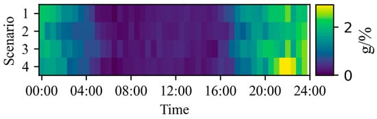
Figure 8.
Heatmap of PIRL superiority deviation.
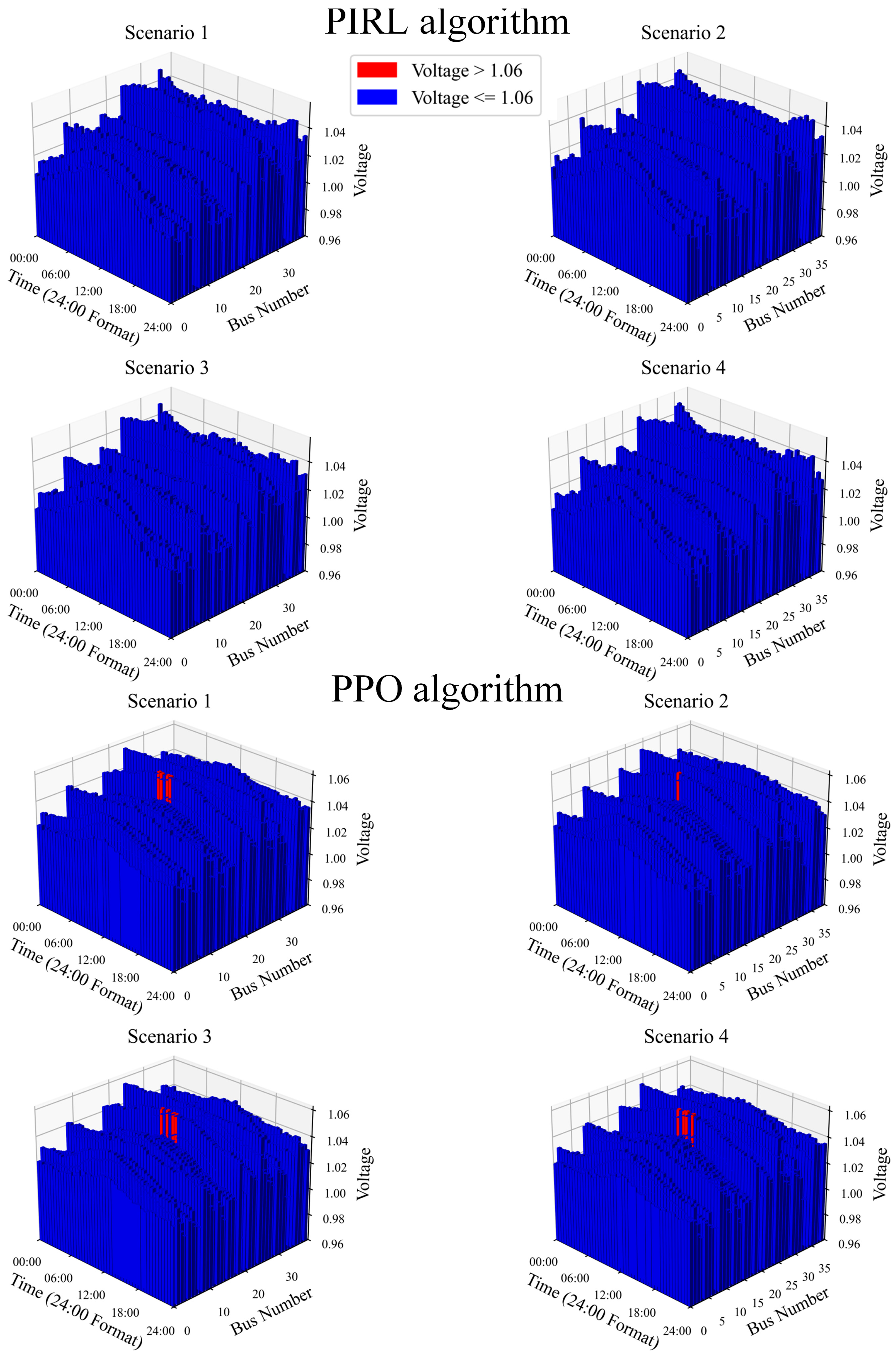
Figure 9 provides a detailed comparison for a representative scenario to further validate the physical feasibility and security of the dispatch solutions, illustrating key power flow results—the node voltage magnitudes and unit power outputs—obtained from the PIRL algorithm and the PPO baseline. The dispatch strategy from the trained PIRL algorithm ensures that both the unit outputs and node voltages adhere to their constraints, guaranteeing system security. In contrast, the PPO algorithm exhibits several limit violations.
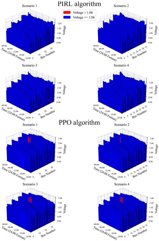
Figure 9.
Power flow simulation results under PIRL and PPO.
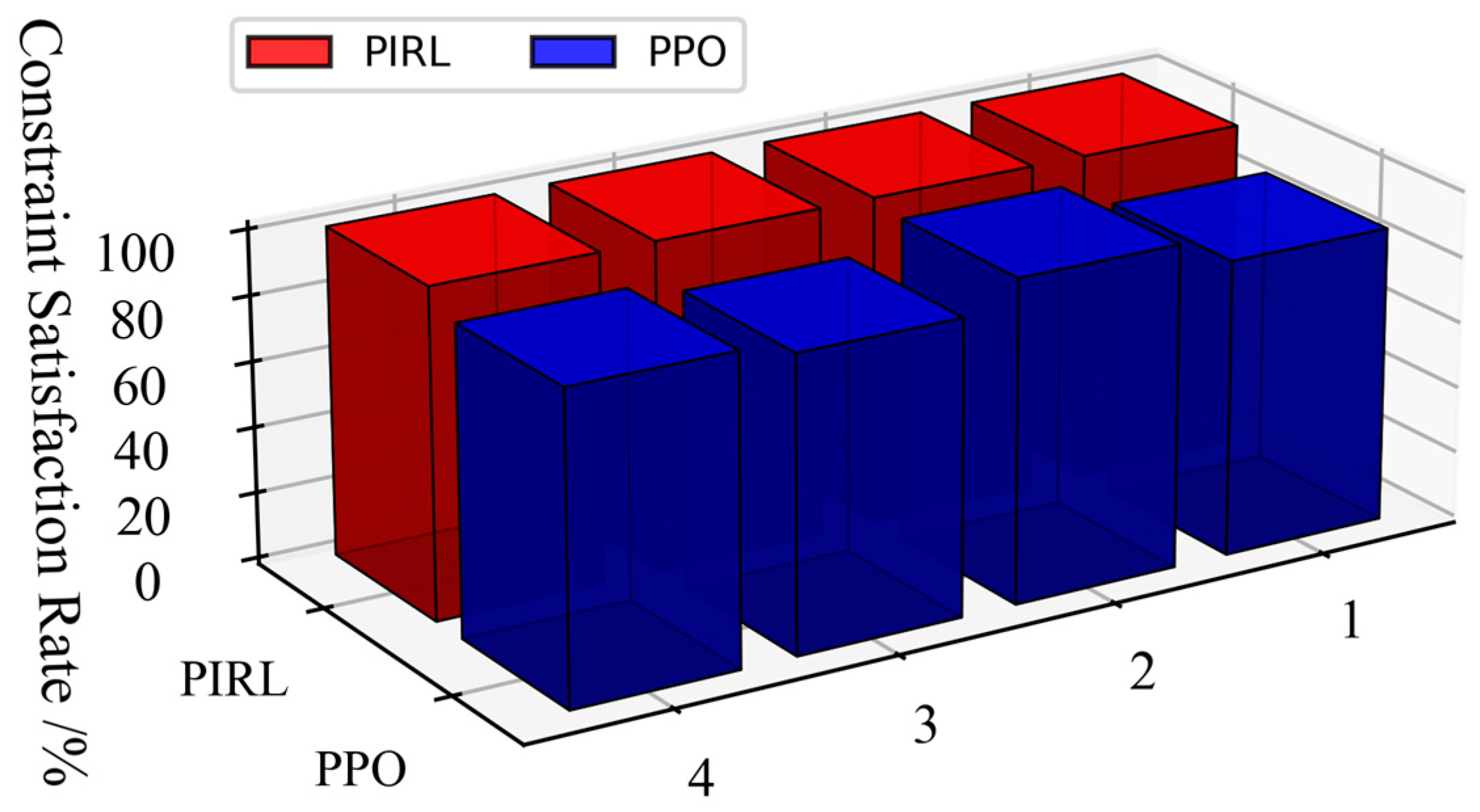
By statistically analyzing the constraint violation of dispatch decisions of each dispatch interval made by different algorithms across the four scenarios (Figure 10), the PPO algorithm exhibits minor limit violations, whereas the PIRL algorithm successfully ensures all dispatch decisions strictly adhere to operational safety constraints without violations. Furthermore, a comprehensive performance comparison between the two algorithms is summarized in Table 2, covering metrics of optimality, security, and computational speed. In terms of speed, both the PIRL and PPO algorithms achieve millisecond-level decision times (approximately 8 ms), significantly outperforming the traditional interior point method (426 ms). Beyond this shared efficiency, the analysis demonstrates that the PIRL algorithm achieves statistically significant superiority over PPO in both safety compliance and optimality. This evidence highlights PIRL’s enhanced capability to balance economic objectives with rigorous safety guarantees in power system dispatch tasks.

Figure 10.
Statistical plot of constraint satisfaction rate.
Table 2.
Optimality and security comparison analysis.
5. Conclusions and Discussion
In this paper, a Markov decision model is established based on a real-time OPF problem of a power system, and the PIRL algorithm is formed by injecting a physical knowledge regularization term into the actor network of the PPO algorithm, effectively solving the real-time scheduling problem. The superiority of the proposed method is verified by testing in the IEEE 39-bus system.
Compared with the classic PPO algorithm, guided by the exploration through the regularization terms, the learning and exploration efficiency of the PIRL algorithm is improved in the early training stage. In addition, explicit physical knowledge can establish the direct connection between the target and the action, which can improve the convergence ability and the credibility of the neural network in the late training stage.
At the same time, the proposed algorithm has limitations, such as its reliance on a single form of physical knowledge injection. Thus, more embeddable knowledge and embedding methods need to be further explored in subsequent research.
Author Contributions
Conceptualization, X.Z. and X.M.; Methodology, X.Z. and Y.Y.; Software, X.M.; Validation, C.Z.; Formal analysis, D.Y. and Z.L. (Zhida Lin); Investigation, Z.L. (Zhuohuan Li); Resources, X.M.; Writing—original draft, X.Z. and X.M.; Writing—review & editing, X.M. and C.Z.; Visualization, H.X.; Supervision, X.M. All authors have read and agreed to the published version of the manuscript.
Funding
This research was funded by the Innovation Project of China Southern Power Grid Ltd., titled “Key Technologies for Stability Analysis and Coordinated Control of New-Type Power Systems Based on Data-Mechanism Fusion”, grant snumber ZBKJXM20232027.
Data Availability Statement
The original contributions presented in this study are included in the article. Further inquiries can be directed to the corresponding author.
Conflicts of Interest
Authors Ximing Zhang, Yun Yu, Zhida Lin, Huan Xu were employed by the China Southern Power Grid Ltd. Authors Xiyuan Ma, Duotong Yang, Changcheng Zhou and Zhuohuan Li were employed by the Digital Grid Research Institute, China Southern Power Grid. The remaining authors declare that the research was conducted in the absence of any commercial or financial relationships that could be construed as a potential conflict of interest.
References
- Zhang, M.; Han, Y.; Liu, Y.; Zalhaf, Y.L.; Zhao, E.; Mahmoud, K. Multi-Timescale Modeling and Dynamic Stability Analysis for Sustainable Microgrids: State-of-the-Art and Perspectives. Prot. Control Mod. Power Syst. 2024, 9, 1–35. [Google Scholar] [CrossRef]
- Brinkel, N.B.G.; Gerritsma, M.K.; Alskaif, T.A.; Lampropoulos, I.; Voorden, A.M.V.; Fidder, H.A.; Sark, W.G.J.H.M.V. Impact of rapid PV fluctuations on power quality in the low-voltage grid and mitigation strategies using electric vehicles. Int. J. Electr. Power Energy Syst. 2020, 118, 105741. [Google Scholar] [CrossRef]
- Zhao, S.; Shao, C.; Ding, J.; Hu, B.; Xie, K.; Yu, X. Unreliability Tracing of Power Systems for Identifying the Most Critical Risk Factors Considering Mixed Uncertainties in Wind Power Output. Prot. Control Mod. Power Syst. 2024, 9, 96–111. [Google Scholar] [CrossRef]
- Singh, P.; Kumar, U.; Choudhary, N.K.; Singh, N. Advancements in Protection Coordination of Microgrids: A Comprehensive Review of Protection Challenges and Mitigation Schemes for Grid Stability. Prot. Control Mod. Power Syst. 2024, 9, 156–183. [Google Scholar] [CrossRef]
- Xiao, J.; Zhou, Y.; She, B.; Bao, Z. A General Simplification and Acceleration Method for Distribution System Optimization Problems. Prot. Control Mod. Power Syst. 2025, 10, 148–167. [Google Scholar] [CrossRef]
- Milano, F. Continuous Newton’s Method for Power Flow Analysis. IEEE Trans. Power Syst. 2009, 24, 50–57. [Google Scholar] [CrossRef]
- Ponnambalam, K.; Quintana, V.H.; Vannelli, A. A fast algorithm for power system optimization problems using an interior point method. IEEE Trans. Power Syst. 1992, 7, 892–899. [Google Scholar] [CrossRef]
- Narimani, M.R.; Molzahn, D.K.; Davis, K.R.; Crow, M.L. Tightening QC Relaxations of AC Optimal Power Flow through Improved Linear Convex Envelopes. IEEE Trans. Power Syst. 2025, 40, 1465–1480. [Google Scholar] [CrossRef]
- Wang, Q.; Lin, C.; Wu, W.; Wang, B.; Wang, G.; Liu, H. A Nested Decomposition Method for the AC Optimal Power Flow of Hierarchical Electrical Power Grids. IEEE Trans. Power Syst. 2024, 38, 2594–2609. [Google Scholar] [CrossRef]
- Chowdhury, M.M.-U.-T.; Biswas, B.D.; Kamalasadan, S. Second-Order Cone Programming (SOCP) Model for Three Phase Optimal Power Flow (OPF) in Active Distribution Networks. IEEE Trans. Smart Grid. 2023, 14, 3732–3743. [Google Scholar] [CrossRef]
- Huang, Y.; Ju, Y.; Ma, K.; Short, M.; Chen, T.; Zhang, R.; Lin, Y. Three-phase optimal power flow for networked microgrids based on semidefinite programming convex relaxation. Appl. Energy 2022, 305, 117771. [Google Scholar] [CrossRef]
- Li, S.; Gong, W.; Wang, L.; Gu, Q. Multi-objective optimal power flow with stochastic wind and solar power. Appl. Soft Comput. 2022, 114, 108045. [Google Scholar] [CrossRef]
- Nguyen, T.T.; Nguyen, H.D.; Duong, M.Q. Optimal power flow solutions for power system considering electric market and renewable energy. Appl. Sci. 2023, 13, 3330. [Google Scholar] [CrossRef]
- Ehsan, A.; Joorabian, M. An improved cuckoo search algorithm for power economic load dispatch. Int. Trans. Electr. Energy Syst. 2015, 25, 958–975. [Google Scholar]
- Yin, X.; Lei, M. Jointly improving energy efficiency and smoothing power oscillations of integrated offshore wind and photovoltaic power: A deep reinforcement learning approach. Prot. Control Mod. Power Syst. 2023, 8, 1–11. [Google Scholar] [CrossRef]
- Fang, G.; Xu, Z.; Yin, L. Bayesian deep neural networks for spatio-temporal probabilistic optimal power flow with multi-source renewable energy. Appl. Energy 2004, 353, 122106. [Google Scholar]
- Zhen, F.; Zhang, W.; Liu, W. Multi-agent deep reinforcement learning-based distributed optimal generation control of DC microgrids. IEEE Trans. Smart Grid 2023, 14, 3337–3351. [Google Scholar]
- Zhang, K.; Zhang, J.; Xu, P.; Gao, T.; Gao, W. A multi-hierarchical interpretable method for DRL-based dispatching control in power systems. Int. J. Electr. Power Energy Syst. 2023, 152, 109240. [Google Scholar] [CrossRef]
- Rahul, N.; Chatzivasileiadis, S. Physics-informed neural networks for ac optimal power flow. Electr. Power Syst. Res. 2022, 212, 108412. [Google Scholar]
- Nellikkath, R.; Chatzivasileiadis, S. Physics-Informed Neural Networks for Minimising Worst-Case Violations in DC Optimal Power Flow. In Proceedings of the 2021 IEEE International Conference on Communications, Control, and Computing Technologies for Smart Grids (SmartGridComm), Aachen, Germany, 25–28 October 2021; pp. 419–424. [Google Scholar]
- Lakshminarayana, S.; Sthapit, S.; Maple, C. Application of Physics-Informed Machine Learning Techniques for Power Grid Parameter Estimation. Sustainability 2022, 14, 2051. [Google Scholar] [CrossRef]
- Stiasny, J.; Misyris, G.S.; Chatzivasileiadis, S. Physics-Informed Neural Networks for Non-linear System Identification for Power System Dynamics. In Proceedings of the 2021 IEEE Madrid PowerTech, Madrid, Spain, 28 June–2 July 2021; pp. 1–6. [Google Scholar]
- Zeng, Y.; Xiao, Z.; Liu, Q.; Liang, G.; Rodriguez, E.; Zou, G. Physics-informed deep transfer reinforcement learning method for the input-series output-parallel dual active bridge-based auxiliary power modules in electrical aircraft. IEEE Trans. Transp. Electrif. 2025, 11, 6629–6639. [Google Scholar] [CrossRef]
- Wu, Z.; Zhang, M.; Gao, S.; Wu, Z.G.; Guan, X. Physics-Informed Reinforcement Learning for Real-Time Optimal Power Flow with Renewable Energy Resources. IEEE Trans. Sustain. Energy 2025, 16, 216–226. [Google Scholar] [CrossRef]
- Zhao, P.; Liu, Y. Physics informed deep reinforcement learning for aircraft conflict resolution. IEEE Trans. Intell. Transp. Syst. 2021, 23, 8288–8301. [Google Scholar] [CrossRef]
- Biswas, A.; Acquarone, M.; Wang, H.; Miretti, F.; Misul, D.A.; Emadi, A. Safe reinforcement learning for energy management of electrified vehicle with novel physics-informed exploration strategy. IEEE Trans. Transp. Electrif. 2024, 10, 9814–9828. [Google Scholar] [CrossRef]
- Wu, P.; Chen, C.; Lai, D.; Zhong, J.; Bie, Z. Real-time optimal power flow method via safe deep reinforcement learning based on primal-dual and prior knowledge guidance. IEEE Trans. Power Syst. 2024, 40, 597–611. [Google Scholar] [CrossRef]
- Sutton, R.S.; Barto, A.G. The Reinforcement Learning Problem. In Reinforcement Learning: An Introduction, 2nd ed.; MIT Press: Cambridge, MA, USA, 1998; pp. 51–85. [Google Scholar]
- Sayed, A.R.; Wang, C.; Anis, H.I.; Bi, T. Feasibility constrained online calculation for real-time optimal power flow: A convex constrained deep reinforcement learning approach. IEEE Trans. Power Syst. 2022, 38, 5215–5227. [Google Scholar] [CrossRef]
- Cao, D.; Hu, W.; Xu, X.; Wu, Q.; Huang, Q.; Chen, Z.; Blaabjerg, F. Deep Reinforcement Learning Based Approach for Optimal Power Flow of Distribution Networks Embedded with Renewable Energy and Storage Devices. J. Mod. Power Syst. Clean Energy 2021, 9, 1101–1110. [Google Scholar] [CrossRef]
- Li, H.; He, H. Learning to Operate Distribution Networks with Safe Deep Reinforcement Learning. IEEE Trans. Smart Grid 2022, 13, 1860–1872. [Google Scholar] [CrossRef]
- Yi, Z.; Wang, X.; Yang, C.; Yang, C.; Niu, M.; Yin, W. Real-time sequential security-constrained optimal power flow: A hybrid knowledge-data-driven reinforcement learning approach. IEEE Trans. Power Syst. 2023, 39, 1664–1680. [Google Scholar] [CrossRef]
Disclaimer/Publisher’s Note: The statements, opinions and data contained in all publications are solely those of the individual author(s) and contributor(s) and not of MDPI and/or the editor(s). MDPI and/or the editor(s) disclaim responsibility for any injury to people or property resulting from any ideas, methods, instructions or products referred to in the content. |
© 2025 by the authors. Licensee MDPI, Basel, Switzerland. This article is an open access article distributed under the terms and conditions of the Creative Commons Attribution (CC BY) license (https://creativecommons.org/licenses/by/4.0/).