Hierarchical Charging Scheduling Strategy for Electric Vehicles Based on NSGA-II

Abstract

Electric vehicles (EVs) are gradually gaining high penetration in transportation due to their low carbon emissions and high power conversion efficiency. However, the large-scale charging demand poses significant challenges to grid stability, particularly the risk of transformer overload caused by random charging. It is necessary that a coordinated charging strategy be carried out to alleviate this challenge. We propose a hierarchical charging scheduling framework to optimize EV charging consisting of demand prediction and hierarchical scheduling. Fuzzy reasoning is introduced to predict EV charging demand, better modeling the relationship between travel distance and charging demand. A hierarchical model was developed based on NSGA-II, where the upper layer generates Pareto-optimal power allocations and then the lower layer dispatches individual vehicles under these allocations. A simulation under this strategy was conducted in a residential scenario. The results revealed that the coordinated strategy reduced the user costs by 21% and the grid load variance by 64% compared with uncoordinated charging. Additionally, the Pareto front could serve as a decision-making tool for balancing user economic interest and grid stability objectives.

1. Introduction

In the context of the global energy transition and environmental protection, reducing carbon emissions has become an important goal for all countries. Driven by the dual-carbon strategy, China’s new energy vehicle (EV) fleet will exceed 30 million by 2024 [1], significantly reducing carbon emissions in the transport sector and easing environmental pressure.

However, there is a systemic risk behind this exponential growth of EVs. The rapid growth of electric vehicles (EVs) is fundamentally disrupting traditional operational patterns of power grids, with compound risks posed by large-scale charging demand. First, EV charging loads exhibit significant spatiotemporal imbalances. Refs. [2,3] showed that the charging demand of light-duty EVs in residential areas tends to charge during evening hours when users return home. This pattern strongly correlates with the baseline household electricity demand, resulting in a “peak-on-peak” phenomenon and substantially increasing the peak–valley difference in the load profile [4]. Existing charging infrastructure capacity may face challenges in accommodating the growing demand in this scenario [5,6]. Simultaneously, highway charging stations experience severe power demand fluctuations, with instantaneous surges surpassing 400% of their rated capacity [7], which imposes additional stress on grid regulation systems. These imbalances may lead to critical consequences, including thermal overload, voltage violations, and accelerated degradation of transformer lifespans [8,9,10].

Extensive research has been conducted to address the challenges of electric vehicle adoption from various perspectives, including technological innovation and economic analysis. Ref. [11] presented a multivariable probabilistic model for large-scale EV charging demand in New Zealand. Ref. [12] developed a load prediction method combining the GM(1,1) grey forecasting model and Monte Carlo simulation, classifying EVs into private cars, official cars, buses, and taxis. Ref. [13] proposed a spatiotemporal multitask learning model, optimizing regional EV charging demand prediction accuracy. Ref. [14] developed a Stackelberg game model utilizing real charging data and price elasticity to design time-of-use (TOU) tariffs, including seasonal scenario analysis. Refs. [15,16] adopted dynamic electricity pricing mechanisms, incorporating flexible storage and carbon pricing; these strategies effectively incentivize greater EV involvement. Ref. [17] examined the availability of fast-charging infrastructure in EU countries and evaluated infrastructure development plans under the EU Green Deal. Ref. [18] develops an iterated local search (ILS) algorithm for the eBus charging location problem, optimizing station deployment to minimize charging infrastructure requirements. Ref. [19] proposed a data-driven analytical framework by constructing a semi-Markovian trip-chaining, offering empirical insights for infrastructure deployment. Ref. [20] employed NSGA-II to optimize regional electricity pricing for EV charging, leveraging travel patterns and price elasticity. The model achieved the dual objectives of reducing peak grid load while increasing operator profits.

These studies revealed that charging activities critically influence power demand patterns and infrastructure reliability. In this context, significant research efforts have been devoted to understanding EV–grid bidirectional interactions and developing charging strategies. An optimization strategy based on reinforcement learning was proposed in ref. [21].This strategy formulated the problem as a Markov decision process while considering the uncertainties of user behavior, dynamic price, and battery degradation to minimize the user costs and extend battery lifespan. Ref. [22] proposed a two-stage optimization strategy based on particle swarm optimization. This study integrated road network models and fuzzy algorithms to simulate user travel patterns, then combined these with user elastic demand to optimize the spatiotemporal dynamics of charging and discharging. Ref. [23] evaluated two smart charging strategies, an economic model predictive control for minimizing operational costs and an optimal control with maximum flexibility for balancing cost reduction and grid flexibility. A dual-layer model controlling EV charging through dynamic electricity prices was proposed in ref. [24].The upper layer introduced a real-time pricing mechanism based on the load elasticity to respond to the grid load variation, while the lower layer scheduled EV charging loads using Monte Carlo simulation and genetic algorithms. Ref. [25] introduced rolling horizon scheduling to the aggregated EVs in the electricity exchange market, combining genetic algorithms and model predictive control to balance DNOs’ profits and user charging costs. Ref. [26] proposed a variable power charging strategy utilizing particle swarm optimization to minimize load variance, peak–valley difference, and user costs.Refs. [27,28] employed multiagent reinforcement learning (MARL) by dynamically coordinating charging strategies to reduce costs and shave peak loads. Both achieved real-time optimization through online policy updates and effectively handle grid–EV uncertainties. Ref. [29] employed an improved augmented epsilon-constraint method to coordinate EV charging, optimizing distribution network operator costs, power losses, and EV owner expenses simultaneously within physical grid constraints.

Although previous studies have investigated electric vehicle (EV) charging scheduling, several limitations exist in practical implementation. First, traditional Monte Carlo sampling methods typically consider only the state of charge (SOC) as a single parameter, neglecting the impact of range anxiety on charging demand [30]. As a result, the influence of travel distance on charging behavior should be further explored. Second, for this multiobjective optimization problem, linear weighting with fixed coefficients is often applied to derive optimal solutions. However, this approach fails to adaptively balance user economic interests and grid stability across varying demand scenarios. Additionally, most existing research models charging scheduling at the individual vehicle level, formulating the scheduling variable as a matrix in which each element represents the charging status of a vehicle at each time slot. While this approach enables precise control, the number of decision variables increases exponentially with the scale of EV fleets [27], which may limit the practical applicability of models using this tecnique because of the computational complexity.

To address the above issues, the contributions of this paper are as follows.

• The charging load prediction herein incorporates active charging driven by range anxiety, using fuzzy reasoning to better capture the influence of driving distance on the user demand. Both passive charging (initiated when the battery falls below 20% or 15%) and active charging (triggered by range anxiety) are unified through fuzzy rule modeling.
• A hierarchical optimization-based charging scheduling strategy is proposed. In the upper layer, a multiobjective optimization model is formulated to simultaneously minimize user charging costs and distribution network load deviation.
• Nondominated sorting genetic algorithm II (NSGA-II) is used to solve the multiobjective optimization problem, and the Pareto front is generated to provide multiple scheduling choices for decision makers.
• Decoupling between the objective function solving and the specific scheduling strategy is achieved. The upper-layer model aggregates the individual vehicles and formulates the decision variables as a vector, effectively ensuring computational efficiency in large-scale scenarios. The lower-layer model schedules individual vehicles under an aggregated scheduling strategy from the upper layer to satisfy the constraints and ensure the feasibility of the global solution.

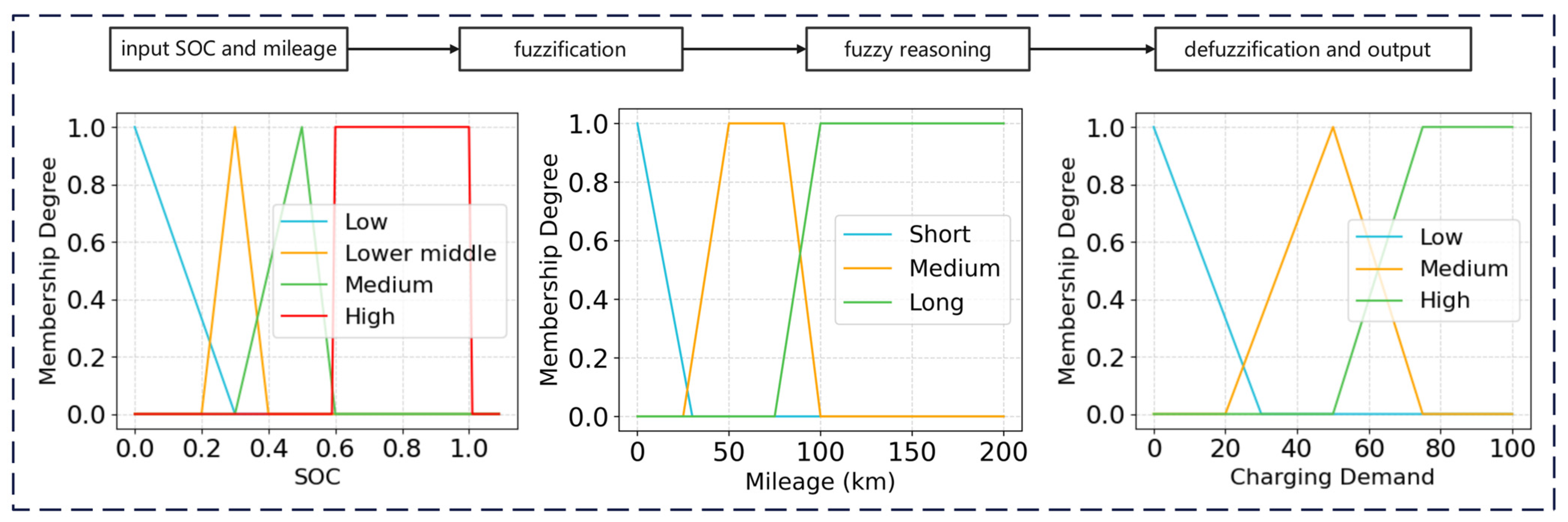
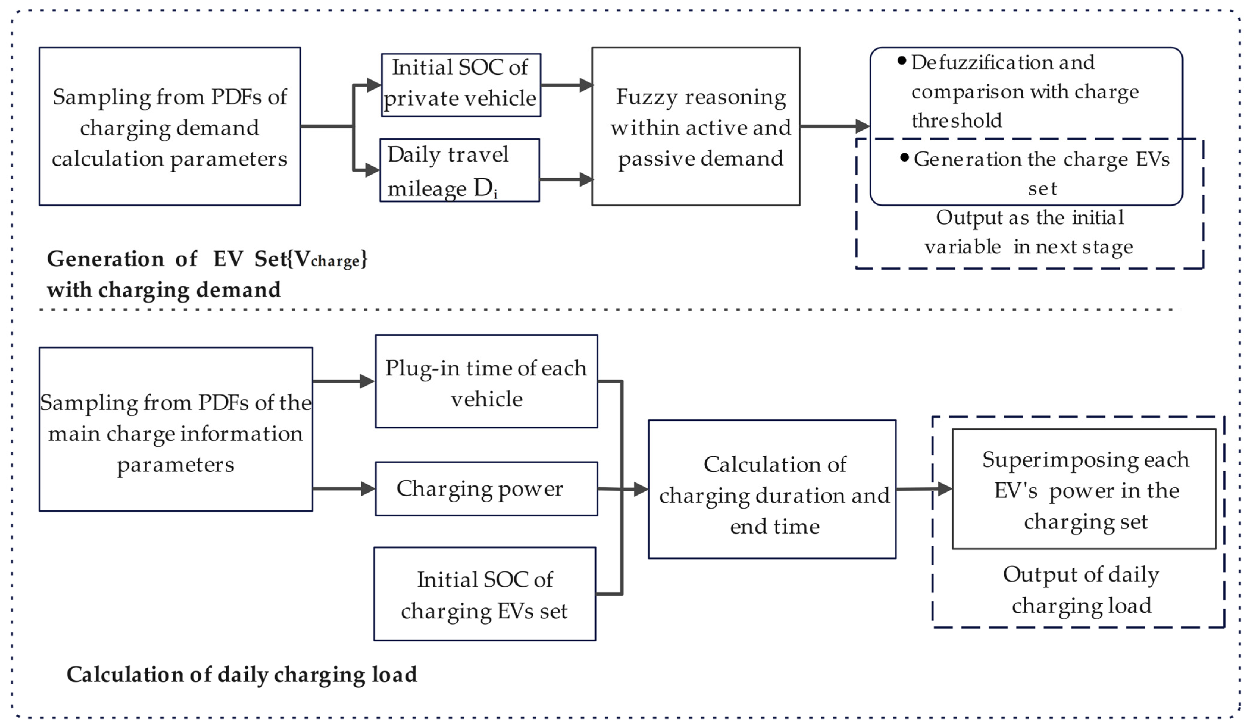
2. Charging Load Prediction

Given that EV endurance mileage is significantly influenced by ambient conditions, many EV owners experience range anxiety and tend to charge their vehicles in advance, even when the state of charge (SOC) remains above the typical low threshold (e.g., 15%) in various situations. This behavior ensures sufficient SOC for the following travel segment.

To address this, an integrated prediction model is proposed that accounts for the impact of range anxiety on charging demand. In addition to passive demand associated with low SOC, the model also incorporates the impact of travel distance on charging demand. The prediction process is structured in two stages: the first stage uses fuzzy reasoning to calculate the charging demand and determine whether the vehicle requires charging; the second stage generates the charging load based on the demand identified in the first stage.

2.1. Fuzzy-Theory Prediction of Charging Demand

Fuzzy algorithms offer broad adaptability for various decision problems, providing a concise representation of complex issues. Variables can be described using natural language terms instead of precise thresholds.

In the proposed charging demand calculation model, state of charge (SOC) and travel mileage were selected as input parameters. Given the substantial differences in daily driving patterns among various types of EVs, it is essential to choose an appropriate EV type for further analysis. Ref. [11] demonstrated that private EVs account for over 80% of mainstream electric vehicle types, with this proportion being even higher in residential areas. Consequently, the simulation model exclusively considers private EVs to more accurately capture charging load characteristics within the target scenario.

According to Ref. [12], the probability density function of private EVs’ SOC is the normal distribution and can be expressed as Equation (1):

$$f_{soc}(x_i)={\displaystyle \frac{1}{\sqrt{2\pi }{\sigma }_{soc}}}\exp \left(-{\displaystyle \frac{{(x_i-{\mu }_{soc})}^2}{2{{\sigma }_{soc}}^2}}\right)$$

(1)

where $x_i$ is the initial SOC value of a single EV, the mean value of initial SOC is ${\mu }_{soc}=0.6$, and the square deviation of SOC is ${\sigma }_{soc}=0.1$.

The distribution of user daily travel distance can be determined by the lognormal distribution function, which can be expressed as Equation (2):

$$f_d(d_i)={\displaystyle \frac{1}{x_d\sqrt{2\pi }{\sigma }_d}}\exp \left(-{\displaystyle \frac{{\left(\ln d_i-{\mu }_d\right)}^2}{2{\sigma }_d^2}}\right)$$

(2)

where ${\mu }_d$ and ${\sigma }_d$ represent the mean value and standard deviation of travel distance, respectively.

The prediction process is shown in Figure 1. The first step involves sampling within the appropriate range of electric vehicle quantities based on the probability density functions of two input parameters. After obtaining SOC and travel mileage, both parameters are divided into multiple segments and assigned to the corresponding evaluation sets for fuzzification.

The calculation process is governed by fuzzy rules with two mandatory boundaries. EVs must charge when the SOC declines to less than 15%, and there is no charging demand when EV SOC exceeds 80%.

Through calculation under the control of fuzzy rules and membership functions, the variable charging demand is defuzzified using the centroid method to obtain a specific value. This value is then compared with a defined threshold. When an electric vehicle’s charging demand exceeds this threshold, it is added to the charging-EV set.

2.2. Charging Load Generation Based on the Sampling and Aggregation

The set of charging EVs established in the previous stage serves as the input in the second stage. The prediction of charge load depends on each EV’s behavior. Consequently, sampling simulation is applied to obtain two variables, plug-in time and charging power, based on corresponding probability density functions.

The plug-in time for private vehicles satisfies a uniform distribution across different periods as introduced in Ref. [12]. The corresponding formulation and distributions are summarized in

Table 1. Distributions of EV charging plug-in times.

Period	Charge Probability	Plug-In Time in Period
8:00–17:00	0.2	Uniform distribution
19:00–6:00	0.7	Uniform distribution
19:00–22:00	0.1	Uniform distribution

.

Regarding charging infrastructure, most public AC chargers are rated between 7 kW and 22 kW, with 7 kW and 11 kW dominating in the market. These chargers are primarily used for slow charging scenarios such as overnight residential and workplace charging [31].

For each charging vehicle, it is reasonably assumed that EV owners will choose to charge until the battery is nearly full. Therefore, the charging duration can be expressed by Equation (3), and the charging end time can be determined by Equation (4).

$$t_{D,i}={\displaystyle \frac{(1-SO{C}_i^s)\times E_b}{P\times \eta }}$$

(3)

where $E_b$ is the battery capacity and $\eta$ represents the charging efficiency;

$${\mathrm{t}}_{e,i}=t_{s,i}+t_{D,i}.$$

(4)

After obtaining the charging behavior of individual EVs, the daily charging load is derived by superimposing all the individual profiles. The generation of the charging-EV set and the load aggregation procedure are illustrated in Figure 2.

3. EV Charging Optimization Strategy

A hierarchical coordinated scheduling model is proposed in this section aiming to achieve a Pareto-optimal solution for balanced optimization of grid operational stability and user economic benefits.

3.1. Upper Layer Model

• Decision Variables

The upper-level model adopts an aggregated scheduling approach with the primary objective of meeting user charging demand. In this strategy, the decision variable is the total charging power allocated to each time interval, which is then provided as input to the lower-level individual scheduling. To ensure scheduling precision, a day is discretized into 96 intervals. Thus, the decision variable is defined as shown in Equation (5):

$$P_j^{EVs}=[p_1^{EVs},p_2^{EVs},\dots ,p_{96}^{EVs}]$$

(5)

• Objective functions

The responsiveness of EV owners is the key factor in the strategy implementation. Consequently, the user charging cost should be minimized, as in the objective function expressed by Equation (6):

$$Min\hspace{0.33em}{F}_1={\displaystyle \sum }_{j=1}^n\hspace{0.33em}\mathrm{Cos}{t}_j^{charge}\times P_j^{EV\mathrm{s}}\times \Delta t$$

(6)

where $\mathrm{Cos}{t}_j^{charge}$ represents the charging price in the jth period under the time-of-use electricity price(CNY/kWh) and $P_j^{EVs}$ denotes the total charging power in the jth period.

To ensure the stability and safe operation of the distribution network, the load fluctuation should be minimized to smooth the load curve. The objective function is expressed by Equation (7):

$$Min\hspace{0.33em}{F}_2={\displaystyle \sum }_{j=1}^n{(P_j^{EVs}+P_j^{base}-P_{mean})}^2/ n$$

(7)

$$P_{mean}={\displaystyle \sum _{j=1}^n(P_j^{EVs}+P_j^{base})}/ n$$

(8)

where n denotes the total number of periods and $P_j^{base}$ and $P_{mean}$ represent the base load of the jth period and the average load across all periods, respectively. The calculation of average load is shown in Equation (8).

• Constraint conditions

The scheduling must satisfy user charging requirements within the distribution network. Based on the previous assumption that users will charge their vehicles to full capacity. This constraint can be expressed as Equation (9):

$${\displaystyle \sum _{j=1}^n{P}_j^{EV\mathrm{s}}}\times \Delta t=\underset{i=1}{\sum ^{N_{EV}}}(1-SO{C}_i^s)\times E_b$$

(9)

where $SO{C}_i^s$ denotes the state of charge of the ith vehicle at the start of charging and $N_{EV}$ is the total number of vehicles in the charging vehicle set.

After EVs are connected, the total load must not exceed the limit of the distribution network limit, and the total charging power should not surpass the capacity of the charging stations. These constraints are expressed by Equation (10) and Equation (11), respectively:

$$P_j^{base}+P_j^{EVs}<P_{max}^{Load}$$

(10)

$$P_j^{EVs}\le P_{max}^c$$

(11)

where $P_{max}^{Load}$ denotes the transformer power limit of the distribution network and $P_{max}^c$ is the capacity of the charging station.

3.2. Lower Layer Model

• Decision Variables

As previously described, the lower-level model schedules the charging of each vehicle within the available power allocated by the upper layer for every time interval. This process optimizes user charging costs and the target state of charge (SOC). To further enhance flexibility, variable charging power is implemented in the scheduling process. The decision variable is expressed by Equation (12):

$${\left[\begin{array}{cccc}{P}_{1,1}^{EV}& P_{1,2}^{EV}& \dots & P_{1,96}^{EV}\\ P_{2,1}^{EV}& P_{2,2}^{EV}& \dots & P_{2,96}^{EV}\\ ⋮& ⋮& \ddots & ⋮\\ P_{n,1}^{EV}& P_{n,2}^{EV}& \dots & P_{n,96}^{EV}\end{array}\right]}_{N\times 96}$$

(12)

where $P_{i,j}^{EV}$ represents the charging power of the ith vehicle in the jth period.

• Constraint conditions

Considering the practical usage of the vehicles, charging is scheduled solely during the parking periods. Additionally, the charging process could be discontinuous. Therefore, the constraint of charging power is expressed by Equation (13):

$$P_{i,j}^{EV}=\left\{\begin{array}{ll}0\hspace{0.33em}\hspace{0.33em}\mathrm{or}\hspace{0.33em}\hspace{0.33em}7\le P_{i,j}^{EV}\le 11,\hfill & \mathrm{if} t_j\in T_{parking}\hfill \\ 0,\hfill & \mathrm{otherwise} \hfill \end{array}\right.$$

(13)

Equation (13) illustrates that the charging power can be flexibly adjusted from 7 kW to 11 kW, allowing for multiphase charging during the parking periods.

The total charging power of the jth period cannot exceed the allocated power from the distribution network. This constraint is expressed by Equation (14):

$${\displaystyle \sum _{i=1}^N{P}_{i,j}^{EV}}\le P_j^{EV\mathrm{s}}$$

(14)

where N is the total number of vehicles and $P_j^{EVs}$ is the allocated power from the upper model for the jth period.

3.3. Multiobjective Optimization Algorithm and Solution Selection

For the high-dimensional optimization problem of charging power allocation, this paper adopts an improved nondominated sorting genetic algorithm (NSGA-II). To avoid the generation of invalid solutions, the algorithm constructs an initial feasible solution set based on the charging demand prediction results presented in Section 2. The Pareto front is obtained using fast nondominated sorting, while crowding distance calculation is applied to maintain the diversity of the solution set in the target space. This approach ensures that the algorithm efficiently generates feasible solutions that minimize the user charging costs and grid load variance.

To select the compromise plan from the numerous solutions, the assessment distance function is defined as Equation (15). This function evaluates each solution based on its distance from the ideal solution:

$$D(x_i)={\omega }_1\times \left[{\displaystyle \frac{F_1(x_i)-F_{1,\min }}{F_{1,max}-F_{1,min}}}-0\right]+{\omega }_2\times \left[{\displaystyle \frac{F_2(x_i)-F_{2,min}}{F_{2,max}-F_{2,min}}}-0\right]$$

(15)

where $x_i$ denotes the ith Pareto solution; $F_{1,min},F_{1,max}$ denote the minimum and maximum user charging costs, respectively; and $F_{2,min},F_{2,max}$ denote the minimum and maximum load variance in the Pareto front, respectively.

The corresponding objective values are first normalized, and then the distance to the ideal solution is calculated to select the compromise solution with the minimum distance. This hierarchical charging optimization process is shown in Figure 3.

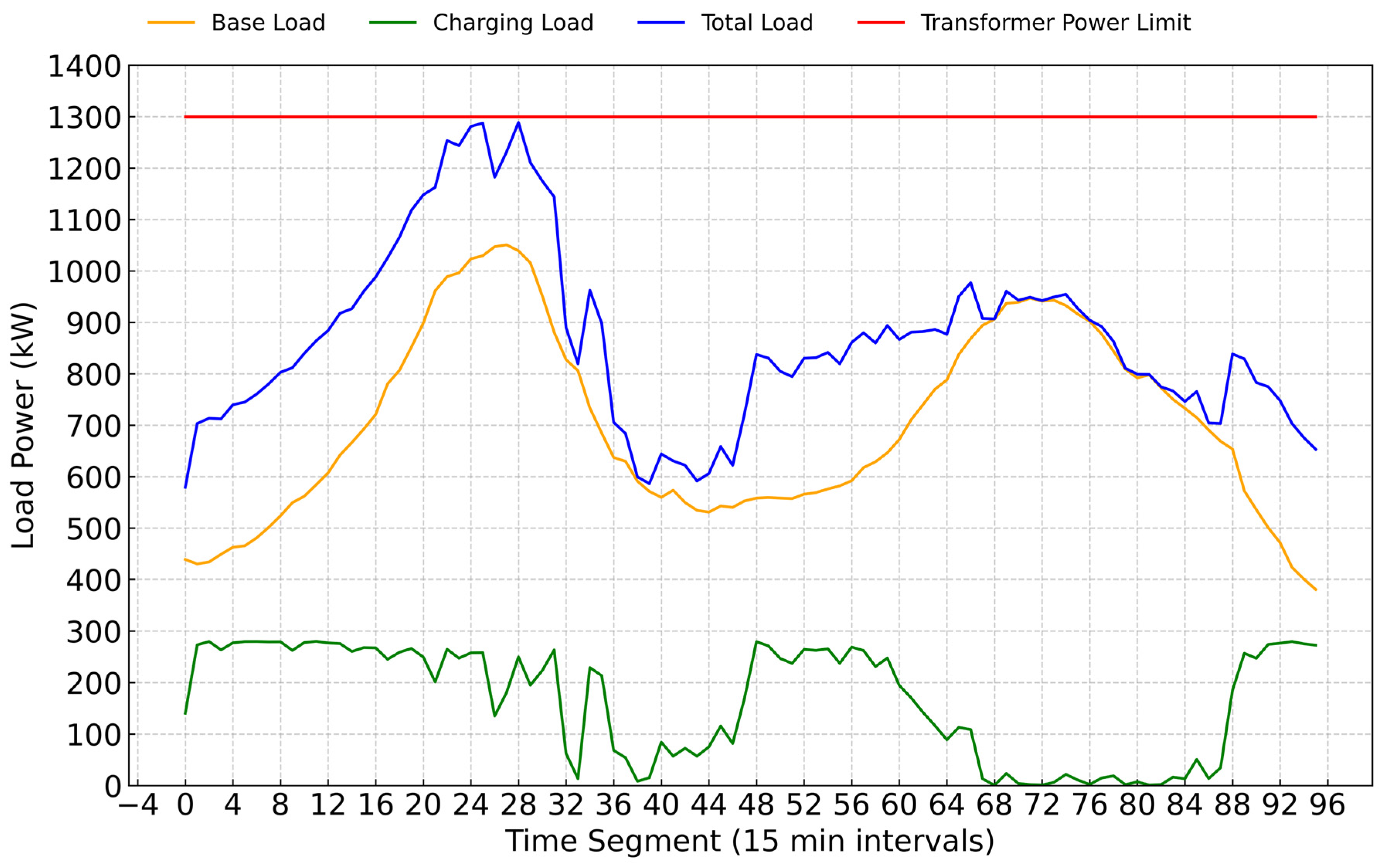
4. Case Study and Analysis

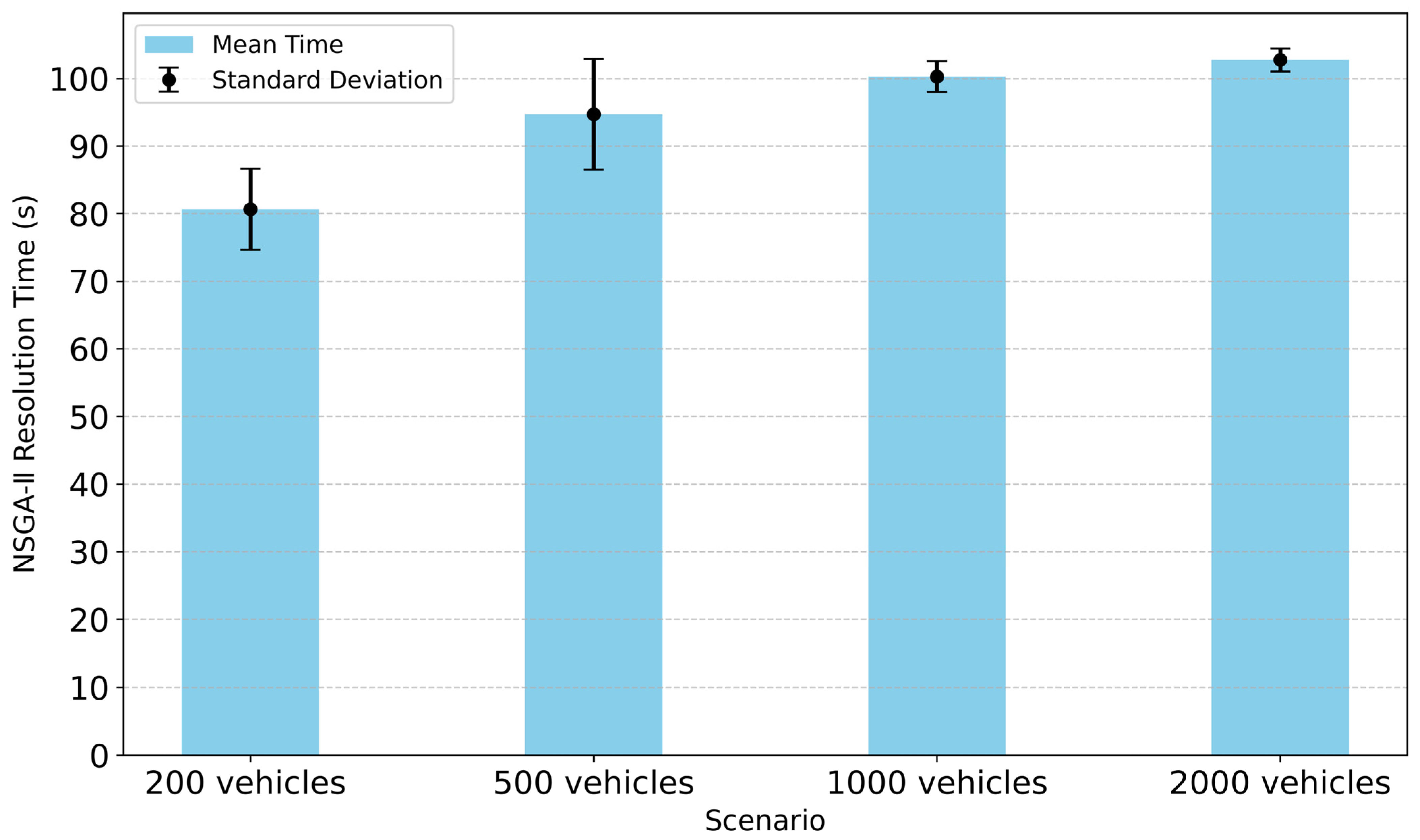
4.1. Computation Comparison Under Different Scenarios

Computation time is a critical factor affecting both the generation and the implementation of scheduling strategies. Figure 4 presents the evaluation results for the hierarchical model under four different EV fleet scales. With the NSGA-II parameters set to a population size of 800 and 600 generations, the results showed that the computation time increased only gradually as the number of vehicles grew, demonstrating that the hierarchical model does not lead to a rapid escalation in computation time with larger fleets.

The total resolution time of the hierarchical model across two EV fleet scales is shown in

Table 2. Computation comparison of hierarchical schedule model under two scenarios.

	Hierarchical Schedule Model
	60 vehicles	200 vehicles
NSGA-II resolution time (s)	68.23	80.64
Individual deployment resolution time (s)	4.73	6.38

. The computation time for the individual vehicle deployment at the lower layer was significantly less than the NSGA-II resolution time. Overall, the hierarchical model could effectively reduce the runtime and mitigate the computational complexity for large-scale scenarios.

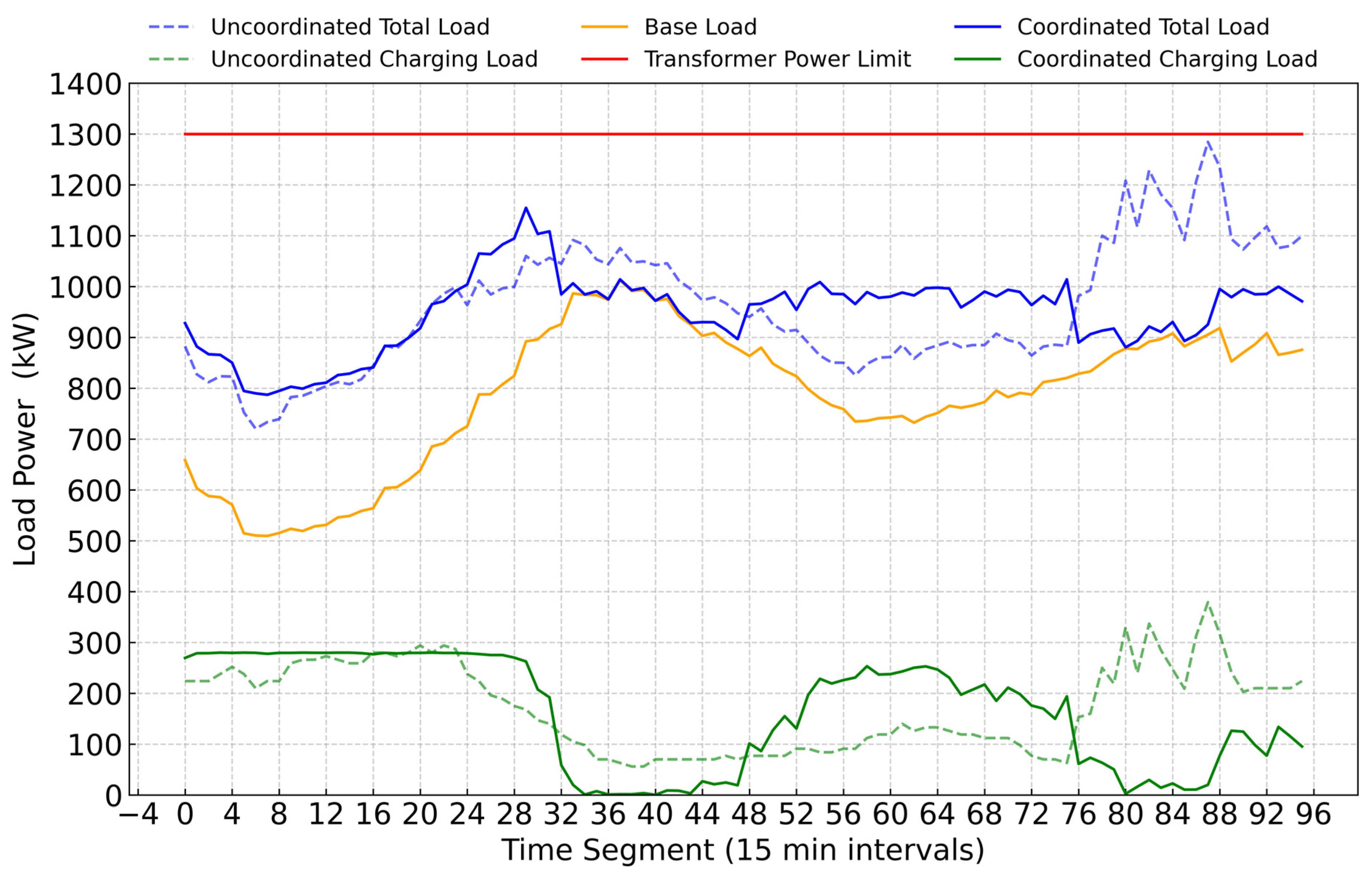
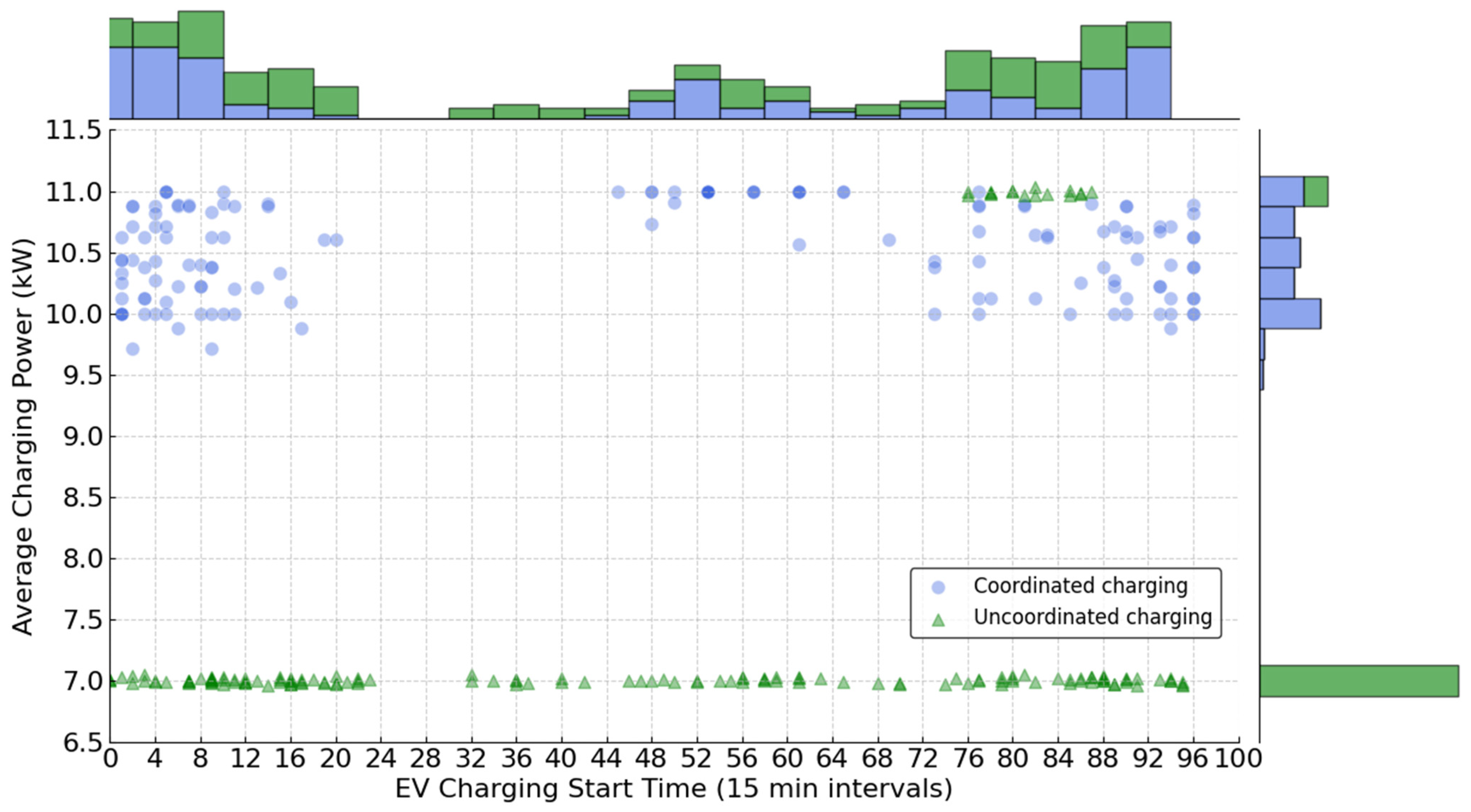
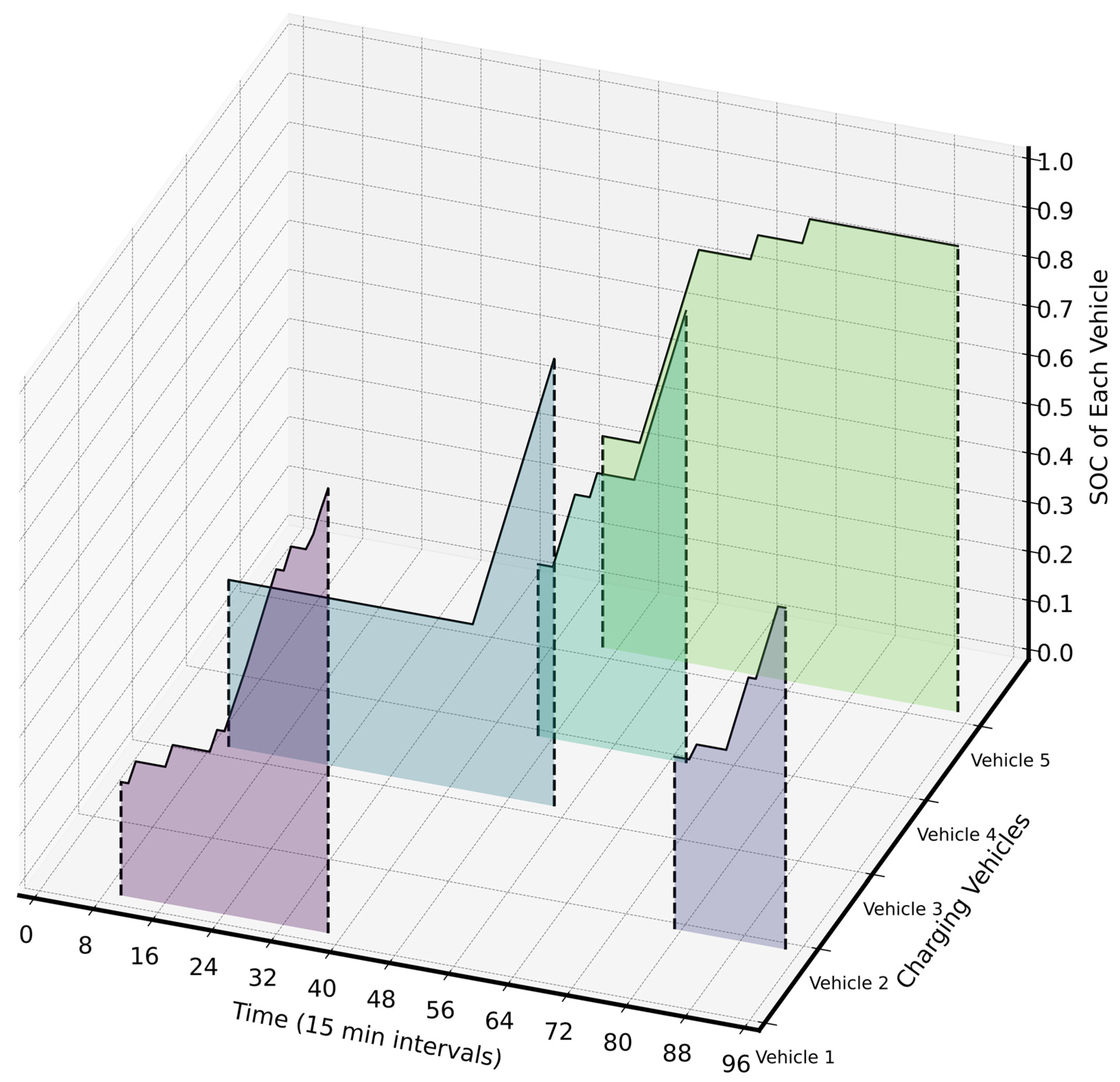
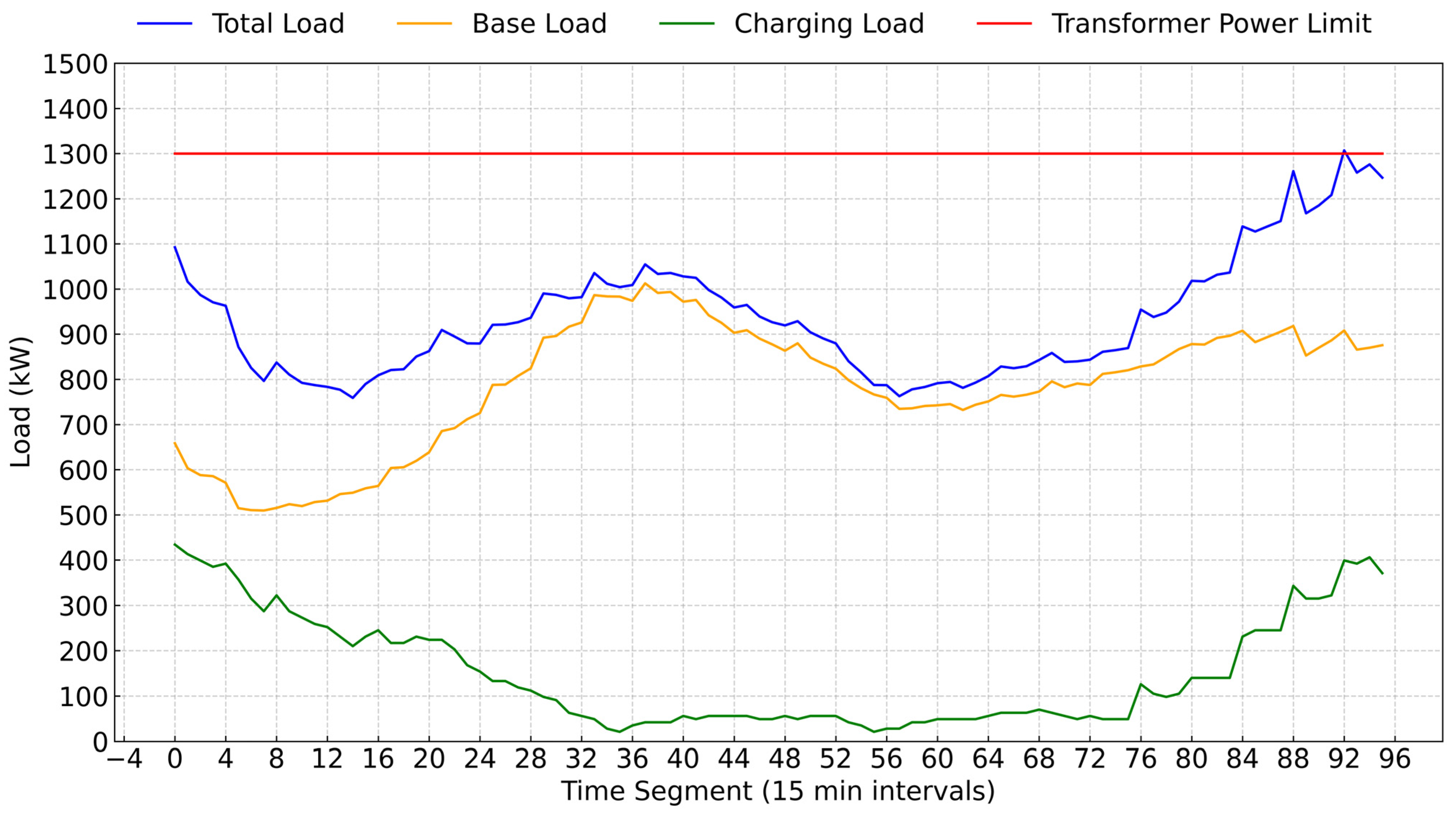
4.2. Case Optimization Results

A residential region served as the target scenario for simulation. The number of electric vehicles was assumed to be 200, and each vehicle was assumed to have a 53 kWh battery. The distribution network had 1300 kW capacity in this region. The time-of-use electricity prices, with three price categories applied, in this residential region are shown in

Table 3. Time-of-use electricity prices.

Type	Corresponding Period	Electricity Price (CNY/kWh)
valley	24:00–8:00	0.332
flat	8:00–9:00 12:00–19:00 22:00–24:00	0.982
peak	9:00–12:00 19:00–22:00	1.382

.

The Pareto front of the biobjective is shown in Figure 5, comprising 165 solutions. The minimum user charging cost was 2495 CNY, and the minimum load variance was 3846 ${\mathrm{kW}}^2$, in this Pareto front.

The selection of the implementation solution was also based on this ideal solution. Since user participation is essential to implement the coordinated charging strategy, the user cost objective was assigned a weighting coefficient as ${\omega }_1=0.7$, while the weight coefficient of grid load variance was ${\omega }_2=0.3$. Solution 1 in Figure 4 was identified as the implementation solution.

4.3. The Optimization Analysis

The load curve under the coordinated charging of solution 1 and the uncoordinated charging is shown in Figure 6. The uncoordinated charging load curve exhibits two distinct peaks in the daily load and the maximum load is close to 1300 kW during the 80th to the 88th period. This phenomenon occurs because the uncoordinated charging behavior closely follows the tendency of base load, resulting in the superimposition of the charging load peak and base load peak and may lead to damage, such as overload risk, increased load fluctuations.

In contrast to uncoordinated charging, coordinated charging could effectively mitigate adverse effects as depicted previously. Most charging power was allocated during the early morning (0th–28th periods) and afternoon (56th–76th periods), thereby avoiding adding new peaks to the existing peak load and shifting charging demand to the trough periods of the base load. As a result, the load curve was smoothed, and the peak–valley difference was reduced. Additionally, the peak load was reduced to approximately 1100 kW, a reduction of 15.4% compared with the peak load under uncoordinated charging. The reduced peak enhances grid hosting capacity and allows for the integration of more electric vehicles.

After the deployment of the lower-layer model, the charging behavior distribution of individual vehicle was generated; this is presented in Figure 7. The results indicated that most vehicles started charging early in the morning, as users typically park in the evening and depart for work next day in residential regions. The available charging power was sufficient in these periods, allowing vehicles to charge to a target state of charge (SOC) before the next trip. Moreover, users could gain economic benefit, since the charging price in this period was low. The average charging power primarily ranged from 10 kW to 11 kW.

Furthermore, this strategy enhanced the flexibility of EV charging compared with conventional continuous charging, as shown in Figure 8, which demonstrates the specific charging process of EVs.

For vehicle 1, the parking hours coincided with the low-electricity-price period, enabling it to be nearly fully charged during the entire parking duration. Vehicle 2 had a relatively short parking period and primarily charged during the flat-price period at maximum power while avoiding charging during the peak price period as much as possible. The parking periods of vehicles 3 and 5 were sufficiently long to allow them to charge during only a portion of their parking period, thereby providing greater flexibility in their charging schedules.

4.4. Comparative Analysis of Different Scenarios

4.4.1. Analysis of Solutions Under Different Weights

The simulation also implemented Solution 2 as shown in Figure 5, which prioritized grid stability compared with Solution 1, with ${\omega }_1$ and ${\omega }_2$ set to 0.1 and 0.9, respectively. The comparison results are summarized in

Table 4. Quantitative comparisons under different load modes.

	Coordinated Charging 1	Coordinated Charging 2	Uncoordinated Charging	Price-Based Uncoordinated Charging	Base Load
User charging cost (CNY)	2560.79	2665.20	3236.18	2714.27	-----
Load variance (kW2)	5.58 × 103	4.30 × 103	1.54 × 104	1.76 × 104	1.92 × 104
Peak–valley load difference (kW)	367.61	282.53	564.07	548.23	503.10

. Both coordinated charging 1 and coordinated charging 2 were beneficial to user economic interest and reduced grid load variance. Compared with uncoordinated charging, user costs and load variance are reduced by 21% and 64% respectively under coordinated charging Solution 1.

Additionally, coordinated charging Solution 2 further smoothed the load curve and reduced the peak–valley load difference, with the load variance and peak valley difference reduced by 72%, and 50% respectively. Moreover, user costs were 18% lower compared with uncoordinated charging.

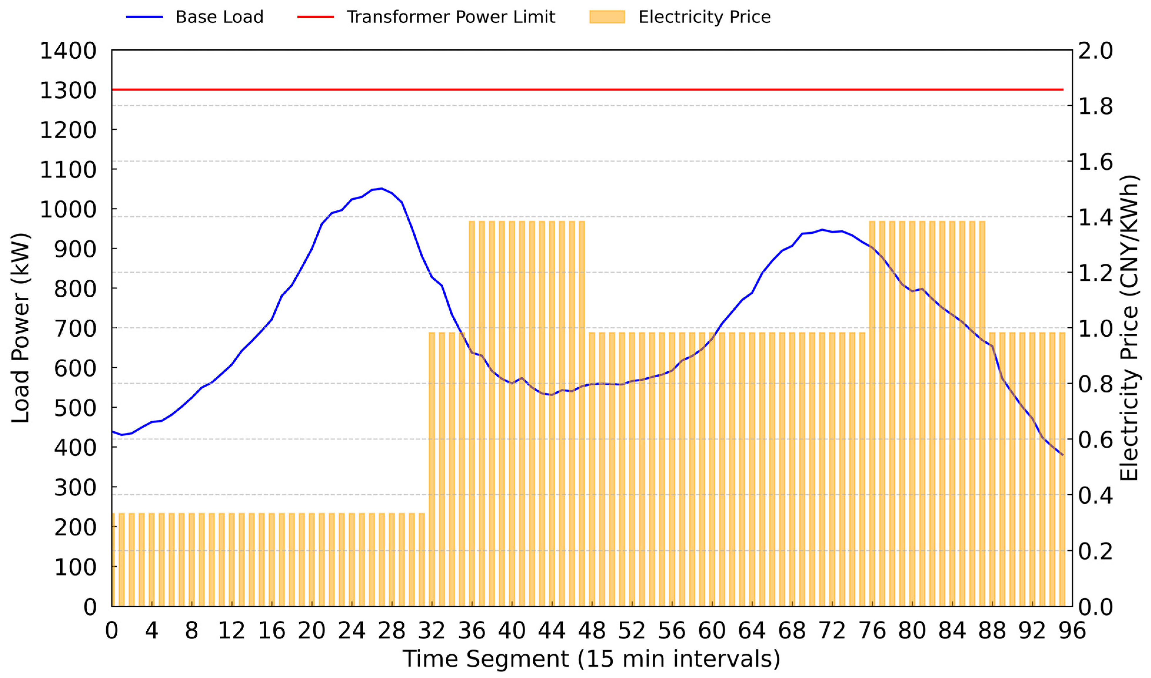
4.4.2. Comparative Analysis with Price-Based Charging Modes

Under the time-of-use electricity price scheme, users tend to concentrate their charging activities during the valley price period. To reflect this behavior, price-based uncoordinated charging was simulated, where 50% of users were assumed to charge their vehicles directly during the valley price period. The resulting load curve is shown in Figure 9. The total load significantly increased during the valley price period because a large proportion of users chose to charge simultaneously. Moreover, the gap between the peak and valley loads was further enlarged. As summarized in Table 4, this charging mode effectively reduced the user charging costs. However, under this mode, the load variance remained similar to that of the base load, indicating that the price-based mode may not effectively mitigate load fluctuations.

4.4.3. Sensitivity Analysis of Base Load

The base load in practice is uncertain, and its peak and valley periods may not exactly coincide with the peak, valley, and flat periods defined by the time-of-use electricity pricing. To evaluate the robustness and adaptability of the proposed charging strategy, a sensitivity analysis was conducted for scenarios where the the peak and valley in base load deviated from the electricity pricing periods, as illustrated in Figure 10.

The corresponding load change is shown in Figure 11, where the load peaks primarily occurred during the 20th–32th and 64th–76th time intervals. During the 20th–28th time intervals, the load curve approached the transformer power limit. This phenomenon occurred because the electricity price was low in this period, leading to a concentration of charging activities.

Moreover, the model still demonstrated notable optimization effects when the base load deviated from the pricing periods; these results are presented in

Table 5. The optimization result under the deviated base load.

	Deviated Base Load	Coordinated Charging
Load variance (kW2)	3.28 × 104	2.98 × 104
Peak–valley load difference (kW)	670.98	709.41

. The load variance was reduced to 2.98 × 10⁴ while maintaining the user charging cost at 2697 CNY, which is 17% lower than that under uncoordinated charging.

5. Conclusions

In this paper, a hierarchical charging optimization strategy is proposed. We formulate the scheduling problem into a dual-layer model. In order to more closely approximate real charging, the projection of charging load utilizes fuzzy reasoning to take into consideration active charging due to range anxiety. In the dual-layer model, the decision variable of the objective function is simplified from the matrix to the vector, which could effectively reduce the computational complexity and be useful in large-scale scenarios. The Pareto front solved by NSGA-II clearly reveals that the balance of user economic interest and grid load fluctuation. Thus, it also could serve as the intuitive basis of two objectives for the decision maker’s selection. From our simulation results, we found that user costs and load variance reduced significantly compared with those under uncoordinated charging. Under Solution 1, the user costs and distribution network load variance decreased by 21% and 64%, respectively, and under Solution 2, which more heavily considered grid stability, the load variance and peak valley difference declined by 72% and 50%, respectively. Overall, these Pareto solutions could be referred to in order to satisfy demand in numerous scenarios.

The limitations of the current model include lacking consideration for the spatial heterogeneity of electric vehicles and not exploring application and analysis across multiple functional zones. This limits its realism and applicability in diverse, real-world scenarios. Future work will focus on incorporating geospatial clustering and developing region-specific scheduling strategies to better reflect the spatial randomness and diversity of EV charging behavior.

This model is currently applied as the day-ahead schedule. The next step could explore real-time scheduling, where the model embeds with model predictive control and updates the planning. Additionally, the proposed model can be extended to coordinate large-scale EV fleets with renewable energy integration, enhancing applicability in sustainable energy systems.

References

1. New Energy Vehicles in Use in China Exceed 30 Million. Available online: https://english.www.gov.cn/archive/statistics/202501/17/content_WS678a06e4c6d0868f4e8eee8a.html (accessed on 23 April 2025).
2. Nizami, M.S.H.; Hossain, M.J.; Mahmud, K. A Coordinated Electric Vehicle Management System for Grid-Support Services in Residential Networks. IEEE Syst. J. 2021, 15, 2066–2077. [Google Scholar] [CrossRef]
3. Zhu, X.; Mather, B.; Mishra, P. Grid Impact Analysis of Heavy-Duty Electric Vehicle Charging Stations. In Proceedings of the 2020 IEEE Power & Energy Society Innovative Smart Grid Technologies Conference (ISGT), Washington, DC, USA, 17–20 February; IEEE: Washington, DC, USA; pp. 1–5.
4. Xiao, Y.; He, C.; Lv, X.; Li, Y.; Zhang, M.; Wang, T. Optimization of Distribution Network Considering Distributed Renewable Energy and V2G of Electric Vehicles. In Proceedings of the 2022 6th International Conference on Power and Energy Engineering (ICPEE), Virtual, 25–27 November 2022; pp. 132–137. [Google Scholar]
5. Ravi, A.; Bai, L.; Wang, H. Optimal Siting of EV Fleet Charging Station Considering EV Mobility and Microgrid Formation for Enhanced Grid Resilience. Appl. Sci. 2023, 13, 12181. [Google Scholar] [CrossRef]
6. Powell, B.; Johnson, C. Impact of Electric Vehicle Charging Station Reliability, Resilience, and Location on Electric Vehicle Adoption; National Renewable Energy Laboratory: Golden, CO, USA, 2024; p. NREL/TP--5R00-89896, 2432350, MainId:90675.
7. Paudel, A.; Sampath, M.; Yang, J.; Gooi, H.B. Peer-to-Peer Energy Trading in Smart Grid Considering Power Losses and Network Fees. In Proceedings of the 2022 IEEE Power & Energy Society General Meeting (PESGM), Chicago, IL, USA, 17–22 July 2022; pp. 4727–4737. [Google Scholar]
8. Mokhtar, M.; Shaaban, M.F.; Ismail, M.H.; Sindi, H.F.; Rawa, M. Reliability Assessment under High Penetration of EVs Including V2G Strategy. Energies 2022, 15, 1585. [Google Scholar] [CrossRef]
9. Yin, W.; Ming, Z. Study on Optimal Scheduling Strategy of Electric Vehicles Clusters in Distribution Power Grid. Optim. Control Appl. Methods 2023, 44, 1769–1778. [Google Scholar] [CrossRef]
10. Barreto, R.; Faria, P.; Vale, Z. Electric Mobility: An Overview of the Main Aspects Related to the Smart Grid. Electronics 2022, 11, 1311. [Google Scholar] [CrossRef]
11. Su, J.; Lie, T.T.; Zamora, R. Modelling of Large-Scale Electric Vehicles Charging Demand: A New Zealand Case Study. Electr. Power Syst. Res. 2019, 167, 171–182. [Google Scholar] [CrossRef]
12. Xing, Y.; Li, F.; Sun, K.; Wang, D.; Chen, T.; Zhang, Z. Multi-Type Electric Vehicle Load Prediction Based on Monte Carlo Simulation. Energy Rep. 2022, 8, 966–972. [Google Scholar] [CrossRef]
13. Shang, Y.; Li, D.; Li, Y.; Li, S. Explainable Spatiotemporal Multi-Task Learning for Electric Vehicle Charging Demand Prediction. Appl. Energy 2025, 384, 125460. [Google Scholar] [CrossRef]
14. Zheng, Z.; Zheng, C.; Wei, Z.; Xu, L. Analysis of Charging Tariffs for Residential Electric Vehicle Users Based on Stackelberg Game. Energy Rep. 2024, 12, 1765–1776. [Google Scholar] [CrossRef]
15. Mahdi, M.A.; Abdalla, A.N.; Liu, L.; Ji, R.; Bian, H.; Hai, T. Optimizing Microgrid Load Fluctuations through Dynamic Pricing and Electric Vehicle Flexibility: A Comparative Analysis. Energies 2024, 17, 4994. [Google Scholar] [CrossRef]
16. Zhang, L.; Yin, Q.; Zhu, W.; Lyu, L.; Jiang, L.; Koh, L.H.; Cai, G. Research on the Orderly Charging and Discharging Mechanism of Electric Vehicles Considering Travel Characteristics and Carbon Quota. IEEE Trans. Transp. Electrific. 2024, 10, 3012–3027. [Google Scholar] [CrossRef]
17. Szumska, E.M. Electric Vehicle Charging Infrastructure along Highways in the EU. Energies 2023, 16, 895. [Google Scholar] [CrossRef]
18. Loaiza Quintana, C.; Climent, L.; Arbelaez, A. Iterated Local Search for the eBuses Charging Location Problem. In Parallel Problem Solving from Nature—PPSN XVII.; Rudolph, G., Kononova, A.V., Aguirre, H., Kerschke, P., Ochoa, G., Tušar, T., Eds.; Lecture Notes in Computer Science; Springer International Publishing: Cham, Switzerland, 2022; Volume 13399, pp. 338–351. ISBN 978-3-031-14720-3. [Google Scholar]
19. Liu, Z.; Borlaug, B.; Meintz, A.; Neuman, C.; Wood, E.; Bennett, J. Data-Driven Method for Electric Vehicle Charging Demand Analysis: Case Study in Virginia. Transp. Res. Part D Transp. Environ. 2023, 125, 103994. [Google Scholar] [CrossRef]
20. Wang, R.; Mu, J.; Sun, Z.; Wang, J.; Hu, A. NSGA-II Multi-Objective Optimization Regional Electricity Price Model for Electric Vehicle Charging Based on Travel Law. Energy Rep. 2021, 7, 1495–1503. [Google Scholar] [CrossRef]
21. Maeng, J.; Min, D.; Kang, Y. Intelligent Charging and Discharging of Electric Vehicles in a Vehicle-to-Grid System Using a Reinforcement Learning-Based Approach. Sustain. Energy Grids Netw. 2023, 36, 101224. [Google Scholar] [CrossRef]
22. Zhang, L.; Sun, C.; Cai, G.; Koh, L.H. Charging and Discharging Optimization Strategy for Electric Vehicles Considering Elasticity Demand Response. eTransportation 2023, 18, 100262. [Google Scholar] [CrossRef]
23. Diaz-Londono, C.; Maffezzoni, P.; Daniel, L.; Gruosso, G. Comparison and Analysis of Algorithms for Coordinated EV Charging to Reduce Power Grid Impact. IEEE Open J. Veh. Technol. 2024, 5, 990–1003. [Google Scholar] [CrossRef]
24. Yang, X.; Niu, D.; Sun, L.; Ji, Z.; Zhou, J.; Wang, K.; Siqin, Z. A Bi-Level Optimization Model for Electric Vehicle Charging Strategy Based on Regional Grid Load Following. J. Clean. Prod. 2021, 325, 129313. [Google Scholar] [CrossRef]
25. Su, J.; Lie, T.T.; Zamora, R. A Rolling Horizon Scheduling of Aggregated Electric Vehicles Charging under the Electricity Exchange Market. Appl. Energy 2020, 275, 115406. [Google Scholar] [CrossRef]
26. Ji, Y.; Zhang, J.; Li, S.; Deng, Y.; Mu, Y. Variable Power Regulation Charging Strategy for Electric Vehicles Based on Particle Swarm Algorithm. Energy Rep. 2022, 8, 824–830. [Google Scholar] [CrossRef]
27. Shen, X.; Zhang, Y.; Wang, D. Online Charging Strategy for Electric Vehicle Clusters Based on Multi-Agent Reinforcement Learning and Long–Short Memory Networks. Energies 2022, 15, 4582. [Google Scholar] [CrossRef]
28. Huang, S.; Yang, M.; Yun, J.; Li, P.; Zhang, Q.; Xiang, G. A Data-Driven Multi-Agent PHEVs Collaborative Charging Scheme Based on Deep Reinforcement Learning. In Proceedings of the 2021 IEEE/IAS Industrial and Commercial Power System Asia (I&CPS Asia), Chengdu, China, 18 July 2021; IEEE: Piscataway, NJ, USA, 2021; pp. 326–331. [Google Scholar]
29. Wang, Y.; Wang, H.; Razzaghi, R.; Jalili, M.; Liebman, A. Multi-Objective Coordinated EV Charging Strategy in Distribution Networks Using an Improved Augmented Epsilon-Constrained Method. Appl. Energy 2024, 369, 123547. [Google Scholar] [CrossRef]
30. Thorhauge, M.; Rich, J.; Mabit, S.E. Charging Behaviour and Range Anxiety in Long-Distance EV Travel: An Adaptive Choice Design Study. Transportation 2024. [Google Scholar] [CrossRef]
31. Global EV Outlook 2024. Available online: https://www.iea.org/reports/global-ev-outlook-2024 (accessed on 16 June 2025).
Figure 1. The fuzzy reasoning process and membership function.
Energies 18 03269 g001
Figure 2. The process diagram of charging load prediction.
Energies 18 03269 g002
Figure 3. The diagram of hierarchical charging schedule strategy implementation process.
Energies 18 03269 g003
Figure 4. NSGA-II computation time under varying vehicle scenarios.
Energies 18 03269 g004
Figure 5. Pareto front of grid load variance and user charging costs.
Energies 18 03269 g005
Figure 6. Load curve under coordinated and uncoordinated charging modes.
Energies 18 03269 g006
Figure 7. Scatter plot of charging start time and power distribution in the two charging modes.
Energies 18 03269 g007
Figure 8. Typical optimized charging process under coordinated charging.
Energies 18 03269 g008
Figure 9. Load curve under price-based uncoordinated charging.
Energies 18 03269 g009
Figure 10. The relationship between time-of-use electricity price and the deviated base load.
Energies 18 03269 g010
Figure 11. Load curve with a deviated base load under coordinated charging.
Energies 18 03269 g011