Contextual Analysis of Battery Electric Vehicles’ Adoption in Italy

Abstract

This study investigates the context in which the adoption of battery electric vehicles (BEVs) takes place in Italy. Several region-specific characteristics pertaining to socioeconomic conditions, transportation, and infrastructure are studied and combined by means of Principal Component Analysis (PCA) and k-means clustering. The model acts as a tool able to provide a 3D visualization of the relative states of the 20 regions analyzed. Three Principal Components are computed, and seven clusters are identified and described, with Lombardy, Trentino-South Tyrol, Aosta Valley, and Lazio showing an advanced level of adoption compared to the rest of Italy. Key findings indicate that regional incentives are necessary to accelerate adoption in underperforming regions, and that incentives targeting the scrapping of old vehicles might not always be useful. To address the emerging disparities, recommendations tailored to the individual territories are provided.

1. Introduction

Despite tentatively dating back to the first half of the eighteenth century, battery electric vehicles (BEVs) are only nowadays taking up larger and larger shares of international markets in the automotive field. With studies on technology and innovations being continuously produced, major manufacturers such as BYD, Tesla, and Volkswagen are developing new models each year, reducing the impact of concerns such as range limitations and charging time. In addition to the manufacturers’ push, and especially in urban contexts, BEVs are expected to play an ever-growing role due to their ability to avoid most local emissions during motion, which is recognized as being of utmost importance to address in the wider context of decarbonization. As a matter of fact, in 2019, the exhaust emissions coming from the transport sector accounted for 25.9% of the total emissions generated by the EU-27. Since passenger cars are the predominant means of transport, accounting for up to 79.5% of passenger-kilometers, any solution able to lower their emissions will have wide and proficient repercussions on the overall sector’s emissions [1,2].

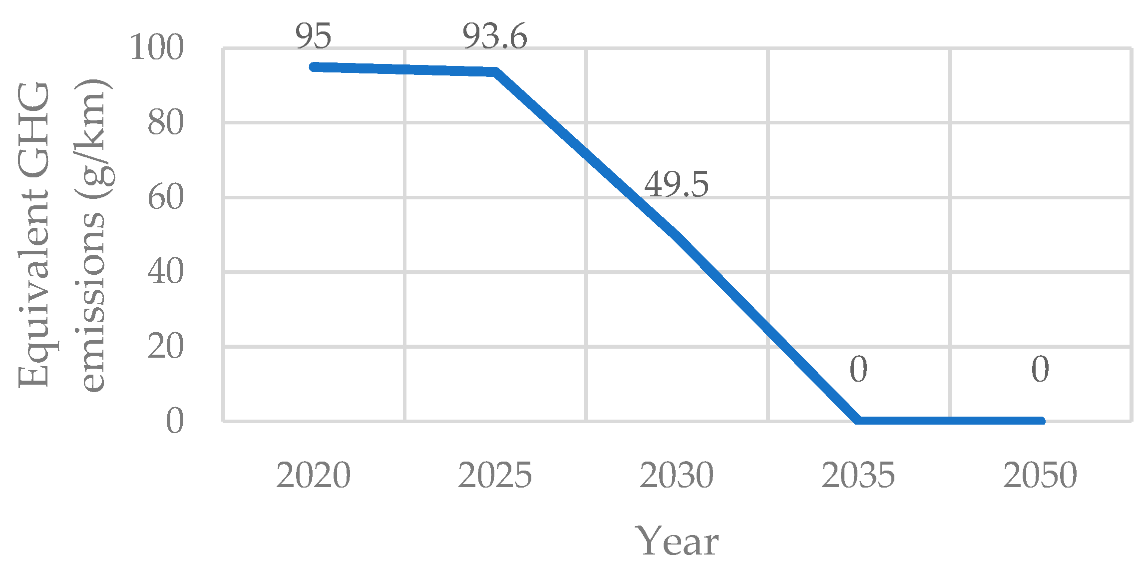
From an institutional point of view, the European Commission has set, by 2035, the target of only producing vehicles able to reduce emissions by 100% compared to 2021, with the intermediate step of reducing them by 55% before 2030 [3]. As is possible to see in Figure 1, this corresponds to dropping from 95 g/km of CO₂ to 49.5 g/km in 2030 and to 0 g/km in 2035.

Other limits have been set for the emissions from vans and heavy-duty vehicles, with the latter being set to a 90% reduction by 2040 [4].

From a strategic point of view, BEVs can be expected to become short-term stationary storage systems if Vehicle-to-Grid solutions become a diffused reality [5], as well as provide information about the infrastructure and communication systems [6]. In addition to this, the uptake of BEVs allows for the development of synergies with other emerging trends and themes, such as in the case of high photovoltaic penetration in the grid, meaning that the surplus generation can be absorbed with smart charging strategies [7], or Autonomous Vehicles, for which intense research is being developed [8,9]. From a legislative, strategic, and manufacturing point of view, BEVs are then supposed to see an increasing international market share on a yearly basis.

However, at the first level of analysis, the global market share expected from the applied top–down manufacturing policies needs to be reflected by the actual uptake of BEVs in all countries part of the Union. If only certain countries can absorb the production of BEVs, the Waterbed Effect occurs, in which the old vehicles will be moved to other countries, thus globally generating more pollutants than expected [10]. This would coincide with a simple relocation of the emissions, without generating any associated reduction. Under these considerations, the actual expected results have to be pursued by guiding markets and incentives in an efficient way, following the actual market share of BEVs on a country-to-country and year-to-year basis. In Italy, the total number of cars has been steadily growing, together with an increase in the average age of the fleet [11]. Despite this, even though the total number of BEVs is growing, their share is yet to change dramatically. Considering that, based on surveys, almost 40% of the population is willing to buy a BEV if it has a cost comparable to an internal combustion engine car [12], incentives in this direction have been applied, with reduced costs in the order of thousands of euros. On the charging side, instead, a conspicuous increase has been seen in charging points, with their presence in the territory growing more than 26-fold [13]. Investments in the field have been studied to make it possible to finance with a payback period of 4–5 years [14].

To what is described above, a second level of analysis of BEV registration shares must be coupled, in which the analysis of the adoption has to be extended to lower territorial administration, to increase the granularity and better understand the possible drivers and barriers. In the following, the registration shares are coupled with socioeconomic, territorial, and demographic variables to give a broader depiction of the phenomenon. The guiding principle of the research is to conduct an analysis in which conclusions can be drawn starting not from a single value, but rather from a regional, multi-variable context highlighted and structured by a mathematical model.

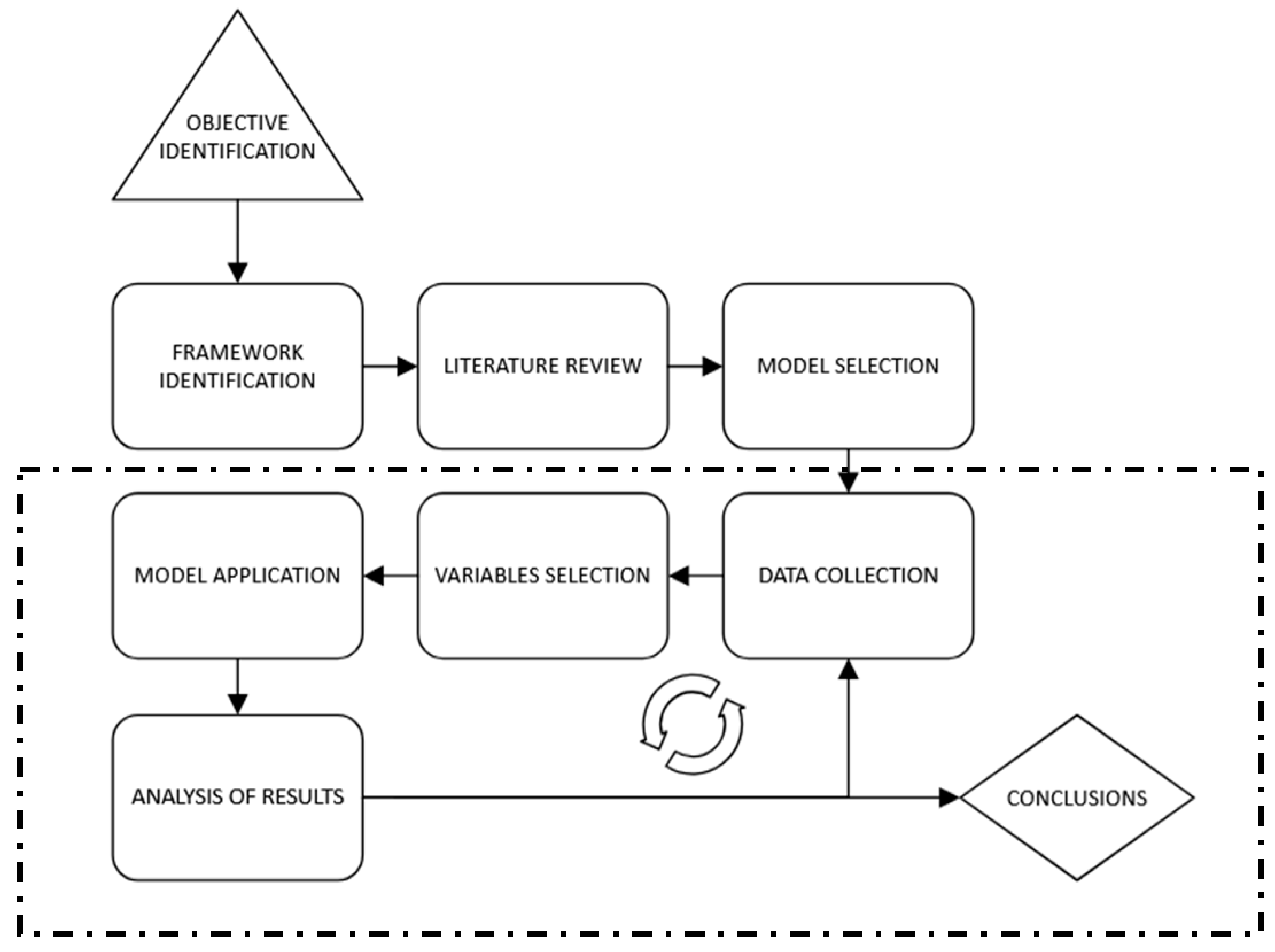
As shown in Figure 2, to support this specific approach and objectives, the research has been structured as follows:

• Objective identification—the scope of the analysis is set after identifying a lack of representation of BEV adoption in Italy.
• Framework identification and literature review—the background information that leads to the model choice and development is studied, and a review of the papers addressing the specific topic of BEV uptake is conducted.
• Model selection, data collection, and variable selection—to analyze the scope set, a variety of models are identified, and one is chosen. Various information has been collected by means of the Italian Statistics Institute and Automobile Club Italia, and an analysis of approximately 30 variables has been conducted to best depict the Italian case of BEV adoption.
• Model application and analysis of results.
• Conclusions and recommendations.

Due to the economic and social relevance of BEVs, the topic has been widely studied in the literature, with several approaches. To support the analysis and the modeling choice of the description of BEV adoption in a territory, a brief literature review has been conducted, with results reported in the following section. In general terms, the main aim of the identified literature was to confront the state of adoption across Europe, both at the international and national levels, as well as to identify which factors could act as facilitators or inhibitors. The variables found in the analysis were many and have been summarized in

Table 1. Summary of some of the variables studied in the research.

Category	Variable	Citation
Economic	Long-term interest rate	[15]
	Average net income index	[16]
	Income distribution by quartiles	[17]
	High purchase price	[18]
	Purchasing power parity	[15]
	Household income	[19]
	Gross domestic product per capita	[17]
	Cost % of mortgage and rent for private	[20]
	Environmental taxes	[17]
	Per capita personal income	[21]
	Median or average personal income	[20,22]
Social	Population density	[16,21,22]
	Share of family households	[16]
	Share of residents × years old and older	[16,21]
	% of people completing higher education	[21]
	Votes for the Green political parties	[16,22]
	Social demographic attributes (gender, age)	[19,20]
	Effort-sharing regulation target for 2030	[15]
	Climate change awareness indicator	[15]
	Education level	[19,20,21,22]
	Proportion of males in population	[19,21]
	Unemployment	[20,21]
Transport	% of cars for commuting	[20]
	Share of one- and two-family houses %	[16]
	Performance-related barriers (e.g., poor acceleration, reduced driving pleasure due to lack of an internal combustion engine)	[18,19]
	Average number of km per day	[22]
	Biofuel usage	[15]
	Usability barriers (e.g., range anxiety)	[18,19]
Technology	Density of public charging points	[15,16,17,22]
	Safety and technology barriers	[19]
	Renewable energy source share	[15,17]
	Ownership of charging outlets	[21,22]
	Number of EV outlets	[20]

.

Studies on BEV adoption employ both statistical and predictive models to analyze influencing factors. Some such as Möring-Martínez et al. [15] study the circumstances of the adoption in various countries by means of PCA, while some make use of spatial statistics to focus on identifying patterns or regression models to predict adoption rates, such as multivariable linear regression [16], spatial Durbin [20], and geographically weighted regression [21]. Across multiple studies, economic factors like income levels and purchase costs are frequently examined. Personal income, whether median or per capita, appears in several analyses [20,21], though its statistical significance varies. In the EU, age was a stronger predictor than income, whereas in the U.S., infrastructure-related factors, such as the number of BEV outlets, played a greater role [21]. Population density is another commonly analyzed variable, with findings indicating higher BEV adoption in urban areas [16,23]. Studies in Germany and the U.K. highlight disparities between rural and urban regions, with adoption rates generally higher in more densely populated areas. Transport-related factors, such as commuting habits and housing types, are also considered, with findings suggesting that individuals living in areas with greater public transport use or more compact housing are more likely to switch to BEVs [16,20]. Charging infrastructure is frequently identified as a key technological factor. Multiple studies assess the density of public charging points, with some confirming its statistical significance in predicting adoption rates [16,21]. Italian survey-based research highlights range anxiety and infrastructure concerns as major barriers [19], alongside subjective factors such as reduced driving pleasure due to the lack of an internal combustion engine. On the topic, the authors of [24] elaborate on Discrete Choice Modeling results to show that among respondents, there is a willingness-to-pay of EUR 80 for each additional km of range, consistent with other results in the literature [25]. Political and demographic factors are also explored. Studies in Germany and Sweden analyze, among others, the correlation between higher BEV adoption rates with electoral support for environmentally focused parties [16,22]. Age demographics appear in multiple analyses, but findings differ; some suggest younger populations are more inclined toward BEVs, while others indicate that age alone is not a decisive factor when economic conditions are accounted for [21]. The geographic scope varies, with some research comparing national markets and others analyzing city-level variations, revealing significant disparities even within the same country. These dimensions of analysis have also been expanded by cultural and behavioral studies. An example of this approach is that of [26] in Trentino-South Tyrol, which tests interventions on the population, aimed at enhancing the behavioral aspects of the uptake by highlighting the cost-saving structure and peer decisions in the same field. Findings on the topic suggest that there is a strong need to thoroughly analyze the context of the interventions due to the high heterogeneity of the respondents [27], as well as the information contained in the norm-based interventions. The authors conclude that a valid approach would be to first target the groups most likely to positively react and then extend to large-scale interventions. Similar single-region research has been conducted by [28], elaborating that at the University of Perugia, students and faculty members share as drivers climate awareness, but they differ in that the former appreciate fuel economy and the latter show frequent car usage. Policies are also widely analyzed as an effective tool to aid the adoption of BEVs, with various studies comparing them across European countries [29] and exploring the most efficient ones [30,31]. Given the results of the literature review, addressing the lack of analysis at the multi-regional level in Italy, and considering that rather low significance has been shown from predictive models, the modeling choice fell on selecting variables able to describe the context in which BEVs are registered. A more in-depth explanation of the characteristics of the data that weaken regressors is provided in Section 2.5.

The research objective, then, is to deepen the understanding of the adoption of BEVs in Italy with a purely descriptive approach, in which the complex dynamics of causality and the possible nonlinear correlation between the variables do not affect the implications of the results. In this light, statistical and mathematical models able to relate variables and give a clearer understanding of the position of each region have been chosen, namely PCA and Clustering. The reason for this choice is that the combination of these two methods allows for a dimensionality reduction with successive partitioning of the space, with sole dependence on the choice of a parameter (k) and the accepted amount of total explained variance of the PCA, which will be explained in depth in Section 2.5.

To summarize, the main contributions to the research are:

• Analyzing the contest and background in which BEV uptake in Italy takes place;
• Developing a Principal Component Analysis with successive clustering on these data, to provide a structured context for peer-to-peer comparison;
• Providing region-specific recommendations to support policy makers in the adoption of BEVs.

2. Modelling Approach and Process

2.1. Theoretical Background

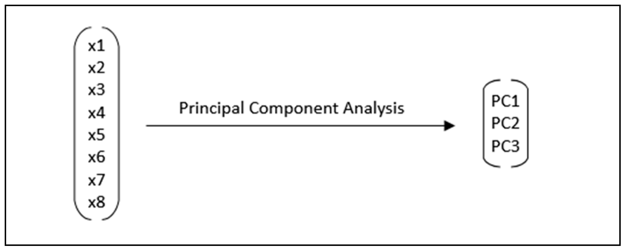
Principal Component Analysis is a dimensionality reduction technique that employs a linear combination of the variables in a dataset. The Principal Components (PCs) correspond to the unit vectors aligned with the direction that maximizes variance, such that after the first component has been identified, a new direction (namely, the Second Principal Component) is computed to capture the largest amount of variance left, and so on. Data have to be standardized to avoid the effects of scale [32]. The n starting variables (and p instances) are reduced to m ending variables at will, under the trade of losing the part of the variance that was captured by the remaining n-m PCs. The way this reduction is achieved is by means of a Factor Loading Matrix, where the n × m matrix represents the coefficients of the linear mapping that elaborates the n variables in the new m variables. In the case of 8 variables, there are 3 Principal Components (Figure 3):

The Factor Loading Matrix contains three elements for each x.

In general, in mathematical notation, let us assume that X is n × p matrix filled with p occurrences of n variables (1), where $x_{ij}$ is the value of the i-th region for the j-th variables:

$$\mathit{X}=\left[\begin{array}{cccc}{x}_{11}& x_{12}& \dots & x_{1n}\\ x_{21}& \dots & \dots & \dots \\ \dots & \dots & \dots & \dots \\ x_{p1}& \dots & \dots & x_{pn}\end{array}\right]$$

(1)

The mean row is computed as (2)

$$\overline{\mathit{x}}={\displaystyle \frac{1}{n}}\sum _{j=1}^n{x}_j$$

(2)

The matrix of mean rows is computed as (3)

$$\overline{\mathit{X}}=\left[\begin{array}{c}1\\ 1\\ \dots \\ 1\end{array}\right]\left[\begin{array}{c}\overline{\mathit{x}}\end{array}\right]$$

(3)

from which the mean-centered matrix B is computed as (4)

$$\mathit{B}=\mathit{X}-\overline{\mathit{X}}$$

(4)

and the Covariance Matrix C (n × n) is (5)

$$\mathit{C}={\mathit{B}}^T\mathit{B}$$

(5)

Given the results above, it is now possible to compute the n eigenvalues and eigenvectors, solving (6)

$$\mathit{C}\mathit{v}=\lambda \mathit{v}$$

(6)

Using the computed eigenvectors, it is possible to apply a rotation of the original dataset into a new projected space, by means of the matrix V_k, filled with k eigenvectors, selected by means of different possible metrics or criteria. By sorting the eigenvectors in descending order and selecting only the k largest, with k < n, the rotation, which at this point is strictly related to the maximization of captured covariance, reduces the dimension of the dataset from n variables to k Principal Components.

$${\mathit{X}}_{\mathit{P}\mathit{C}\mathit{A}}={\mathit{B}\mathit{V}}_{\mathit{k}}$$

(7)

The newly generated ${\mathit{X}}_{\mathit{P}\mathit{C}\mathit{A}}$ is the projection sought.

Following this, k-means clustering is applied. This clustering technique is based on assigning each point to the cluster with the nearest centroid, minimizing the variance within the cluster. Since the number of clusters (k) must be defined beforehand, this technique is usually coupled with other methods to identify the most suitable value of k, such as the elbow method. The choice of the clustering algorithm was guided by the intention of splitting the space itself into specific sectors called Voronoi regions. Other alternatives, such as hierarchical clustering, would instead agglomerate the points based on the relationship between the specific points of the dataset, not directly generating the subdivision of space.

The k-means algorithm can be summarized as follows [33]. First, $K$ centroids are randomly initialized from the given data points, denoted as $C=\{c_1,c_2,\dots ,c_{\mathrm{k}}\}$. The algorithm then iteratively refines these centroids until convergence or until a predefined maximum number of iterations is reached. In each iteration, every data point x_i is assigned to the cluster whose centroid is closest to it, based on the minimum pairwise distance. After the assignment, the centroids are updated by computing the average of all data points assigned to each respective cluster. Finally, convergence can be checked by evaluating whether the centroids have changed significantly; if not, the process is terminated early. Finally, the algorithm returns the resulting clusters and their corresponding centroids.

2.2. Informational Background

To support the methodology and the following models, an analysis of the Italian scenario has been conducted.

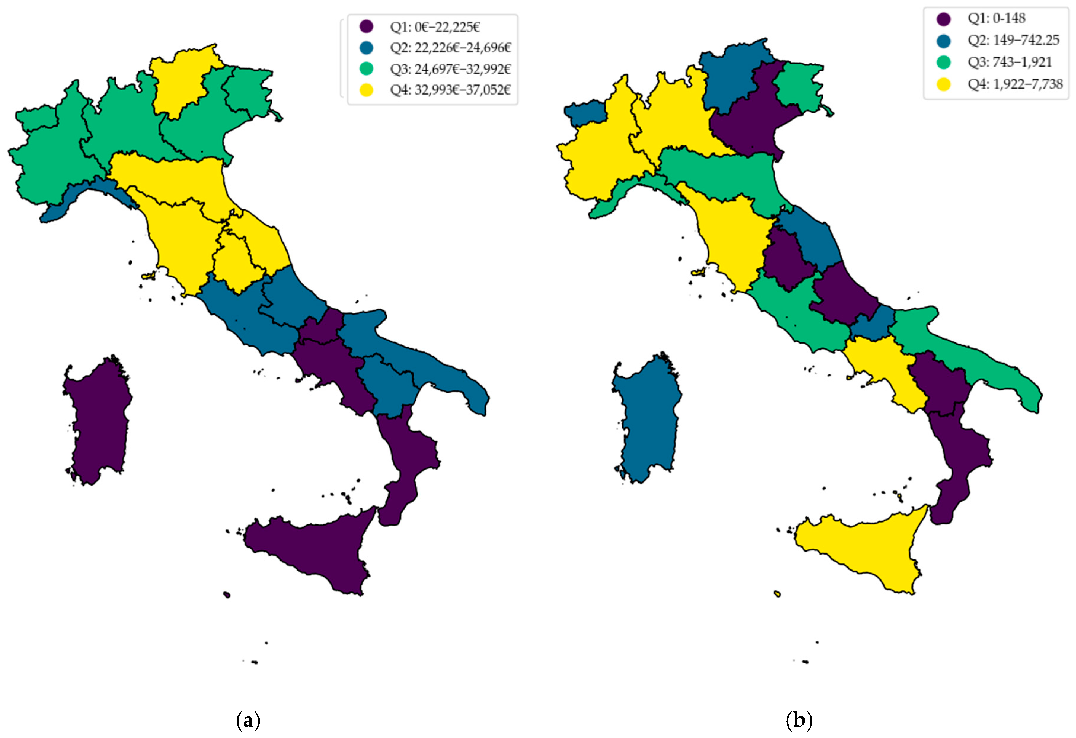
Italy is a country located in the southern part of Europe, facing the Mediterranean Sea, and is organized into 20 regions, 5 of which are regulated by a Special Status: Sicily, Sardinia, Aosta Valley, Friuli-Venezia Giulia, and Trentino-South Tyrol, which is composed of the two Autonomous Provinces Trentino and South Tyrol. In general, a rather substantial difference runs between the Northern, Central, and Southern regions of Italy, as it is possible to see from Figure 4a below, with Southern Italy showing a more complex situation.

Both figures represent the quartile distribution of the values; in purple, the first quartile of the data distribution can be seen, while yellow denotes the upper quartile.

In Figure 4a, it is possible to see how median household income tends to decrease moving towards the South, with the exception of the Liguria region, situated on the northw est coast of Italy. As an example, the main difference with Figure 4b is that the same tendency is not as clear, meaning that general abstractions on multiple variables are not univocally determined. From a historical perspective, many different dominations have occurred across Italy, causing periods of strong development in specific cities (e.g., Palermo (Sicily), Naples (Campania), Bari (Apulia), etc.), which may oppose the general macrotrends of Southern Italy. Referring to socioeconomic, demographic, and technological variables, there exists a great variety across the regions: as an example, the number of electric vehicles registered in 2022 varied between 88 and 8408, while the median household income ranged between EUR 22,225 and 37,052 per year.

Being all regions part of the same country, policies and incentives are the same across Italy. To the best of the authors’ knowledge, the exceptions active as of 2022 are as follows:

• Lombardy and Abruzzo—exempted the vehicle property tax for the years 2022–2024 in case a new, more sustainable car is bought and an old one (e.g., EURO 0 or EURO 1 gas) is scrapped. L’Aquila, the capital of the region, added an additional EUR 4000 incentive for private citizens aiming to buy a BEV.
• Basilicata—supported with contributions only for touristic operators [11].
• Piemonte—only for company vehicles, with a total aid of EUR 8 million.
• Aosta Valley—incentives for 25% of the total price, up to EUR 5000.
• Autonomous Province of Bolzano—EUR 2000 incentive.

Other incentives have alternated over the years in other regions.

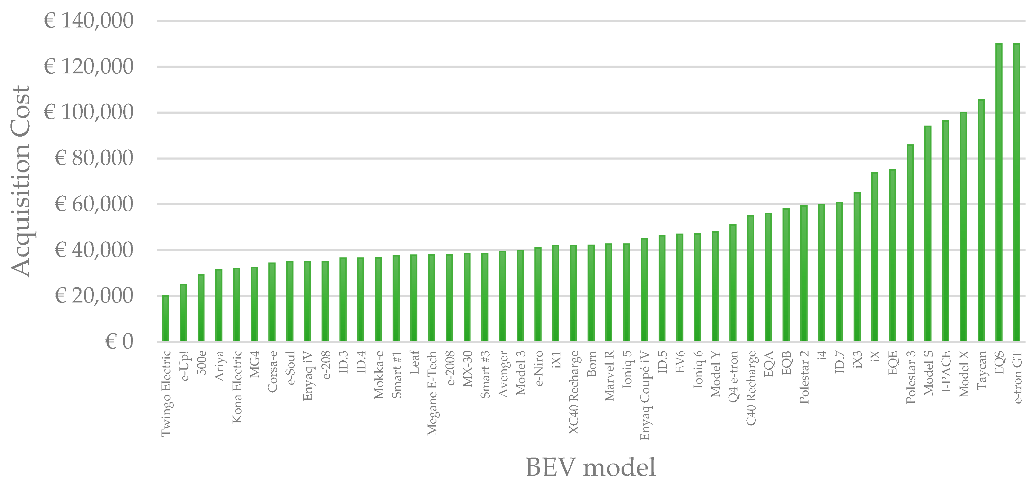
Generally, in the Italian BEV market, most new vehicles fall in the range of EUR 20,000+, as is possible to see in Figure 5 below. Although such vehicles can produce ranges above 180 km, alternatives below this price range see a drastic decrease in km range, such as the Fiat Topolino, priced at EUR 7543 and with a range of approximately 75 km.

2.3. Methodology and Basic Assumptions

The methodology was based on identifying the relevant variables that could influence consumers who are deciding whether to exchange their car in favor of a BEV. Apart from variables of strict regional competence, such as “Provincial and Regional road km”, the choice of variables was modeled on the consumer side, with information able to depict the general status of the population, and the information gathered from the literature. A complete list of the variables considered in the analysis can be found in

Table 2. Summary of the variables analyzed as candidates for this work.

Variable	Description
Region	Label associated with the region
Provincial and Regional Road km	Total amount of road km pertaining to the province and region bodies
Electric Fleet	Total number of existing registered BEVs
Total Vehicle Fleet	Total number of registered vehicles
Number of Charging Points	Total number of charging points for BEVs
Electric Vehicle Registrations	Number of BEVs registered in 2022
% Fleet With Less Than 5 Years	Percentage of total cars (not only BEVs) that are less than 5 years old, used as a proxy for population’s tendency to replace vehicles early
Feet, Vehicle, Driver Car, Passenger	Percentage of the population using the mode of transport for their home-to-work trip
<15 min, >31 min	Average length of home-to-work trips
Improved, Unchanged, Worsened, Much Worse	Perceived variation in household financial status in 2022 compared to 2021
Excellent, Adequate, Poor, Insufficient	Percentage of perceived absolute financial status of the population concerning their expenses
Poverty Risk Percentage	Percentage of the population at poverty risk
Median Annual Household Income (in Euros)	Median annual household income in euros
Area	Square kilometers of the region
Population	Absolute number of residents in the region
Density	Population-to-area ratio in people/km2 for the region
Capital Density	Population-to-area ratio for the region’s capital
Average Rate	Interest rate for the monthly installment of house ownership
Home Loan Installment	Average monthly installment paid by homeowners for financing their house ownership
GDP 2022	Gross domestic product of the region in 2022

. The modeling approach was based on the Italian scenario, such that in a specific region, consumers would be interested in buying (and thus registering) a BEV due to the following:

(1)

Being exposed to the concept or presence of BEVs;

(2)

Feeling safe in changing the current vehicle for a new BEV;

(3)

Being in the financial position to purchase a new BEV;

(4)

Feeling safe in being able to recharge in a public place.

As an example, living in a region where the average age of vehicles is low could mean that there is a naturally high propensity for frequent vehicle change, accelerating the uptake of BEVs. On the other hand, if a large part of the population is at risk of poverty, the region is arguably less likely to see a mass uptake of BEVs.

Some of them, such as “<15 min”, are related to the typical length of the home-to-work trip and are directly obtained by ISTAT, while others, such as “% Fleet with less than 5 years”, had to be elaborated, starting from disaggregated data. Most of the variables are absolute, in the sense that they relate to a specific number (such as absolute number of electric vehicles circulating), while others are comparative, namely “Improved”, “Unchanged”, “Worsened”, or “Much Worse”, which instead refer to the perceived variation in financial conditions for families compared to 2021. The underlying concept was that if, compared to year n − 1, the financial conditions had worsened, it was less likely to see an uptake of statistically more costly vehicles such as BEVs.

All the sources were official and institutional, such as ACI (Automobile Club Italia) and ISTAT (Italian Statistics), and where multiple sources were present, coherence with already-used ones was preferred. The reliability of the data was ensured by choosing 2022 as the timeframe, for which the data collection and analysis from both entities have been completed and stabilized. Although for some variables (not included in this research) both entities have missing points for specific groups or years, all the data reported and used were complete and certified.

2.4. Variable Selection

All the variables were selected with an iterative approach, aimed at maximizing the amount of information without creating excessive redundancy, with the initial pool involving more than 30 elements and the final one having 8.

Different from analyses that tackle the European or international level, when conducting a PCA on a single-nation level, most of the variables were not fit to be selected. An example of this is how GDP refers to sectors such as great industries, with rather little clear propagation of such wealth to the wider population. Due to this, GDP itself was discarded in favor of median household income, better able to depict the financial position of the households. In general, one of the main issues associated with PCA is that the variables are seen as equivalent in power, meaning that although the scope of this study was to analyze the uptake of BEVs, when too many variables were presented, the algorithm was giving equal importance to each and thus diluting the relative coefficients and metrics. As an example, when presented with multiple variables pertaining to the financial state of the regions, larger coefficients were given to such a set of variables, neglecting the influence of our variable of interest. This was also reflected in the correlation values between most of these variables, with very high scores (0.95–0.99) that would contribute with low information while affecting the composition of the PCs. In other words, this meant that to present a combined representation of the variables, the need was to balance two effects: adding as much information as possible and avoiding shifting towards a representation of the state of the regions independent from the BEVs. Finding a cluster of regions in which the financial situation was presented would add little to no information to the research.

Some of the variables present in previous studies were discarded in favor of more informative variables, such as the long-term interest rate, which is implicitly present in the home loan installment variable. Some of them instead were found in the literature and used in this study, such as the percentage of people who drive to work or the number of charging points. Another variable proposed in other studies is population density, as well as the population density in each region’s capital.

With these ideas in mind, and recalling Table 1, the final selection of variables can be found in

Table 3. Final variables chosen for the analysis with associated reasoning.

Variable	Reason
Number of charging points	Representative of the infrastructural support to adoption
Electric vehicle registrations	Variable of interest
% of existing vehicles with less than 5 years	Indicative of the renewal rate of cars
% of travelers who drive a car while going to work	Indicative of the reliance on and role of the private car
Median household income	Indicative of the ability of a household to buy a newer car
Population density	Indicative of the number of people exposed to BEVs and the possible customers of the charging points in the region
Population density in the region’s capital	Indicative of the number of people exposed to BEVs and the possible customers of the charging points in the region’s capital
Home loan installment	Indicative of the monthly financial weight for people living in the region

.

2.5. Data Analysis and Model Development

As previously mentioned, the analysis was conducted in Python 3.12.7, with the help of public libraries such as pandas, geopandas, and sklearn, all popular scientific packages.

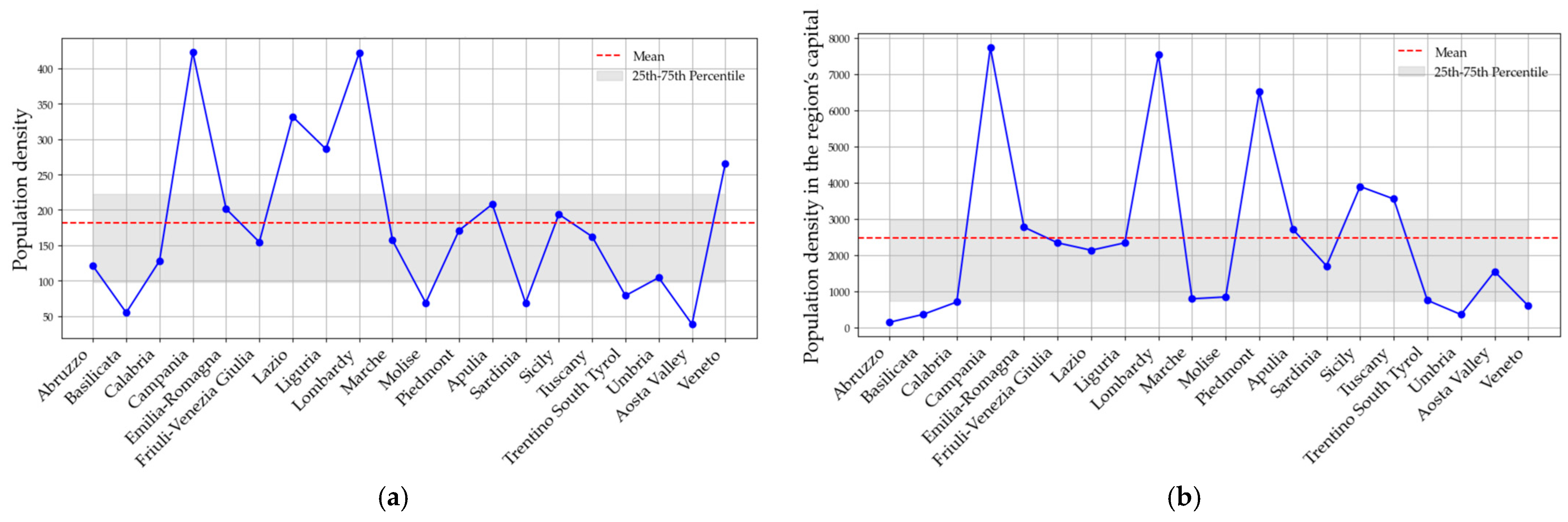
As is possible to see in Figure 6a, population density needed to be coupled with the information pertaining to the region’s capital (Figure 6b), since in some instances, such as Piedmont or Lazio, high values of one of the two did not necessarily mean corresponding high values for the other. In such cases, considering only the population density relative to the overall region would not be able to depict cases in which low-populated regions present high-density capitals, in which the adoption can instead be more proficient. The specific need to consider population density is justified by the close connection it may bear with the social aspects of electric vehicles and the technological aspects of recharging infrastructure. In addition, for some variables, such as median household income, the mean value of the regions was close to the maximum and minimum values, while in others, such as electric vehicle registrations, a much larger gap is present. This makes it particularly hard to draw conclusions based on raw data and calls for the need to establish a method to represent the variables and regions with a structured approach.

As a required step in PCA, data were standardized to avoid effects of scale, meaning that values below average were negative and values above average were positive. Just to give an example, for Abruzzo, there were 832 charging points and −0.671 charging points standardized.

Pearson’s correlation was computed, presented in Figure 7. High values of positive correlation were present for “Electric Vehicle Registrations” and “Number of Charging Points”, as well as for “Population Density” and “Population Density in the region’s capital”. Although with a lower absolute value, negative correlations were also identified, especially between “Home Loan Installment” and “% of travelers that drive a car while going to work”.

Once again, the main issue associated with such an approach is that Pearson’s correlation is particularly valid for linearly correlated variables, which is not the case for these regions. As a matter of fact, correlation does not describe the way the variables act in toto, but the pairwise value that is then referred to as a single value metric.

Having defined and described the variables, Principal Component Analysis and Clustering are conducted in the following section. A reduction to three Principal Components was selected, with an associated Total Explained Variance Ratio (TEVR) of 83.7%, where the TEVR is a measure of the amount of variance explained by the PCA (

Table 4. Explained variance ratio for the first three PCA components.

Principal Component	PC1	PC2	PC3
Explained variance ratio	0.436	0.248	0.153

). This metric is obtained by summing the explained variance of the Principal Components chosen for the analysis and is related to the amount of variance that the new mapping can retain when compared to the initial variables. Another metric used for the selection of the number of PCs is the Kaiser Criterion, which suggests keeping only Components that present an associated eigenvalue larger than 1 [34]. In this specific case, the vector of eigenvalues for the first 4 components is [3.674, 2.089, 1.285, 0.516], meaning that this other approach also suggests that the first three Components are rightful to be kept.

The values of the Explained Variance Ratio (EVR) are rather equilibrated, meaning that although EVR (PC1) > EVR (PC2) > EVR (PC3), the possibility of accepting only one or two Principal Components had to be rejected. In particular, had PC1 and PC2 together accounted for, e.g., 80% of TEVR, PC3 could have been ignored. This not being the case, the three have been rightfully kept and analyzed together.

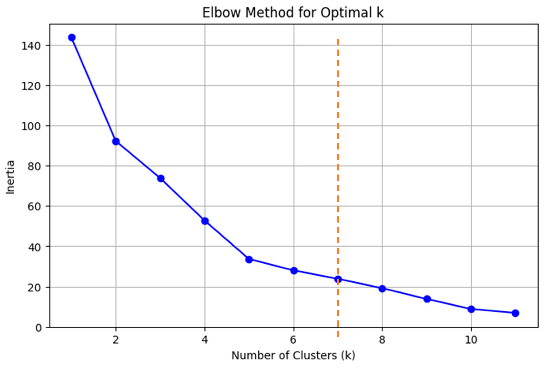
Needing k-means to be provided with the number of clusters, with the help of the Elbow Method, it was set to 7 (see Figure 8).

This number was chosen with the intent of separating differing regions only in case a rather strong difference was present. Once again, negotiation was needed since a too-high number of clusters would add little information, and a too-low one would fail to identify interesting differences. The usage of other criteria, such as silhouette scores, has been avoided due to the restricted number of points and the great variability in their representation.

3. Analysis and Discussion of Results

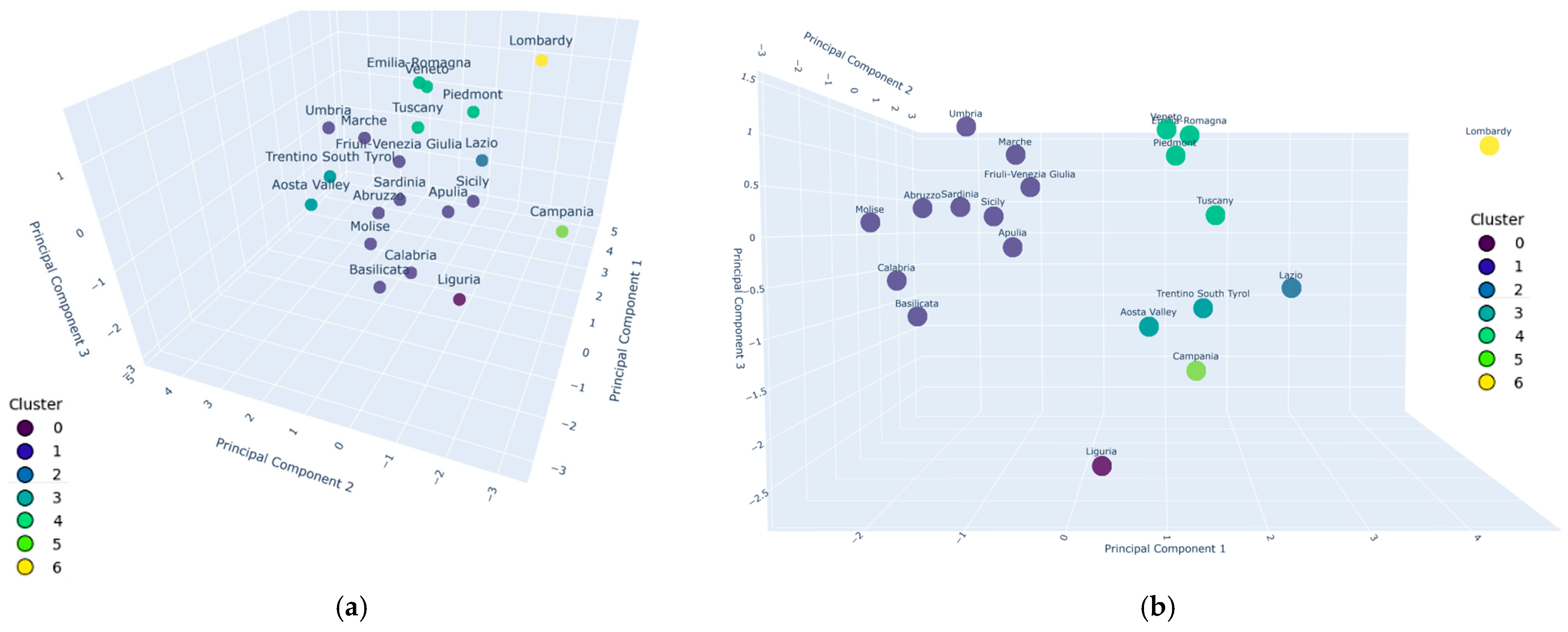
Having reduced the number of components to three, it is now possible to plot them in a 3D space with an acceptable loss of information. In Figure 9, it is interesting to note that k-means correctly separated specific regions from the larger purple cloud on the left: the Lombardy region (yellow), Campania (light green), Liguria (bright purple), and Lazio (blue) are seen as one-point clusters.

In

Table 5. Loadings of the initial variables.

	PC1	PC2	PC3
Number of charging points	0.441	−0.140	0.389
Electric vehicle registrations	0.458	0.176	0.082
% of existing vehicles with less than 5 years	0.212	0.574	−0.256
% of travelers that drive a car going to work	−0.153	0.096	0.805
Median household income	0.290	0.479	0.264
Population density	0.361	−0.460	−0.027
Population density in the region’s capital	0.338	−0.403	0.024
Home loan installment	0.446	0.083	−0.240

, the loadings of different variables with the Principal Components are shown. Of particular importance are elements with an absolute value above 0.3, such as “Number of charging points” for PC1 or “% of travelers that drive a car going to work” for PC3. For the sake of interpretation, we highlighted in green values above 0.3 and in red values below −0.3.

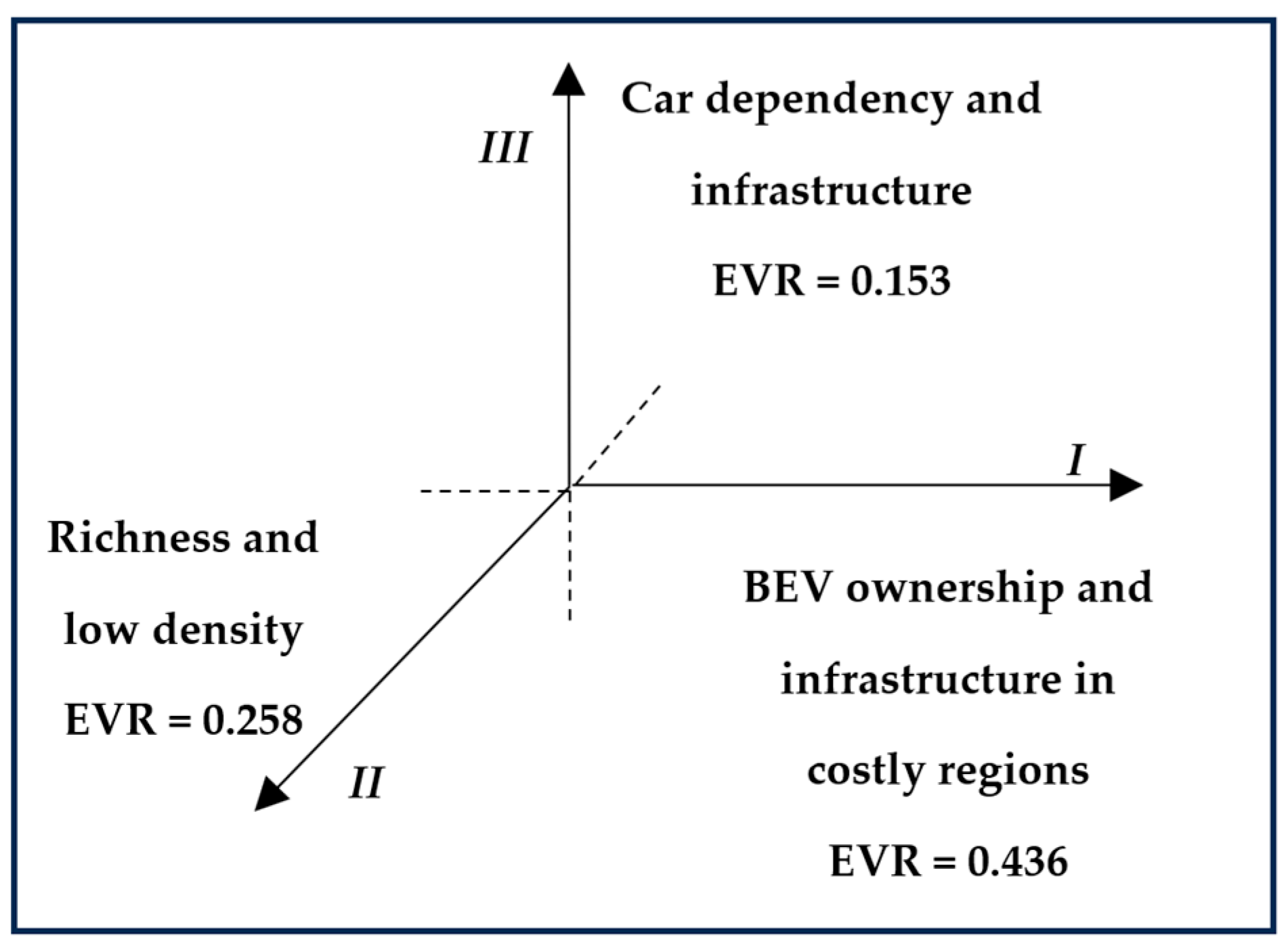
A positive value for Principal Component 1 is associated with high values of “Number of charging points”, “Electric Vehicle Registrations”, “Population Density”, and “Home Loan Installment”. This suggests that a region that presents a high value for Principal Component 1 is a rather technologically advanced one, where there has been interest in and attention towards the topic of BEVs and their uptake, as well as a rather high interest in living in that specific region. Due to these reasons, PC1 could be considered as BEV ownership and infrastructure in costly regions.

A positive value for Principal Component 2 is associated with rather new vehicles (suggesting a high renovation rate), high wages, and low population density, both across the region and the region’s capital. In this case, a high value for the expression of the second PC can be expected for regions that are wealthy and possibly positioned in low-density zones, such as mountainous regions. Due to these reasons, PC2 could be considered as high household income and low population density.

A positive value for Principal Component 3 is associated with strongly car-dependent regions, as well as a high number of charging points. A region that presents high values associated with the third PC can then be thought of as a region in which the strong dependency on cars is coupled with attention to the infrastructural side of the BEV uptake, although such information is not necessarily linked to a corresponding higher uptake of BEVs. Due to these reasons, PC3 could be considered as car dependency and infrastructure (Figure 10).

To give an example of the process of analyzing the results, the cases of Lombardy and Trentino-South Tyrol will be considered.

As is possible to see in

Table 6. Comparative table of Lombardy and Trentino-South Tyrol.

Variable	Mean	Lombardy	Lombardy (std)	Trentino-South Tyrol	Trentino-South Tyrol (std)
Number of charging points	1838.6	5971	2.754	1351	−0.324
Electric vehicle registrations	2448	8205	2.269	8404	2.348
% of existing vehicles with less than 5 years	22.8	24.5	0.110	57.7	2.301
% of travelers that drive a car while going to work	70.9	70.4	−0.073	60.9	−1.393
Median household income	29,137.7	32,485	0.744	37,052	1.760
Population density	181.9	421.9	2.167	78.80	−0.932
Population density in the region’s capital	2469.4	7539	2.222	754	−0.752
Home loan installment	577.1	685	1.413	583.66	0.085

, Lombardy presents a higher-than-average value for all variables except for “% of travelers that drive a car while going to work”, for which a slightly below average value is present, with a corresponding standardized value below 0. The same applies to Trentino-South Tyrol for the variables “Number of charging points”, “% of travelers that drive a car while going to work”, “Population density”, and “Population density in the region’s capital”.

Taking as an example PC2 in

Table 7. Principal Components for Lombardy and Trentino-South Tyrol.

Region	PC1	PC2	PC3	Cluster
Lombardy	4.668	−1.348	1.024	6
Trentino-South Tyrol	1.592	3.230	−1.192	3

, the value for Trentino-South Tyrol is positive also because the standardized values for “Population Density” and “Population Density in the region’s capital” are negative (below the average) and successively mapped by means of a negative coefficient into the new Principal Component coordinate system. This reasoning also shows that, with Lombardy having above-average values for the same variables, the final PC2 value happens to be negative. The sharp difference between the values of PC2 is then to be understood as deriving from the linear combination of the values of all the standardized variables with all the factor loadings, and not a single one-to-one cause–effect. In particular, when tracking the values of PCs, major attention has to be given to the sign of the standardized values and the number of high-value factor loadings associated with the specific PC. Furthermore, when considering PC3, which finds a strong expression in the number of charging points and % of car travelers, that in the former Trentino-South Tyrol is below average and is thus mapped negatively, while in Lombardy it is above average and is thus mapped positively. Despite this, the distance between the two values is further affected by all the other variables and factor loadings, attenuating the strong effect of % of car travelers.

Having explained the process that leads to the creation of Principal Components, an analysis of the clustering is presented, with a brief summary with respect to PCs presented in

Table 8. Summary of the characteristics of the clusters. In brackets is the min–max value of each PC for all regions in the cluster.

Cluster	# Regions	Range PC1	Range PC2	Range PC3
0	1	0.220	−0.911	−2.761
1	10	(−2.709, −0.752)	(−1.457, 1.044)	(−1.034, 1.469)
2	1	2.525	−0.562	−0.644
3	2	(1.593, 0.727)	(3.230, 3.280)	(−1.492, −1.193)
4	4	(0.999, 1.663)	(0.320, 0.803)	(0.260, 1.362)
5	1	1.285	−2.929	−1.328
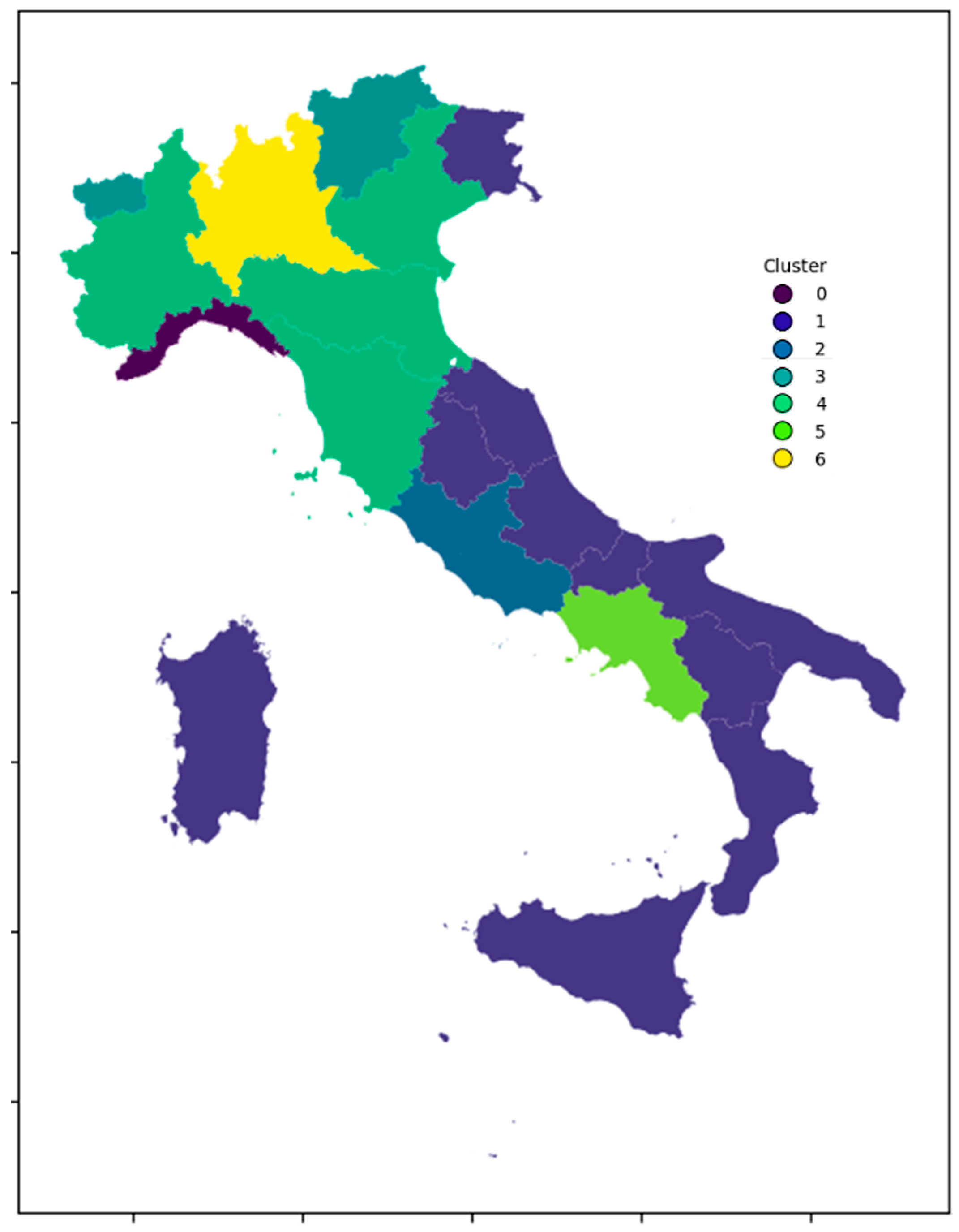
6	1	4.668	−1.348	1.024

. As is possible to see in Figure 11, such aggregations do not represent, as an example, the distributions seen in Figure 4, nor do others, and thus provide a unique visualization of the state of adoption.

Three more-than-single clusters were found (namely Cluster 1, Cluster 3, and Cluster 4), comprising 16 out of 20 regions, meaning that many regions occupy a similar position in the Principal Component space.

On the one hand Cluster 1 alone is composed of 10 regions (Apulia, Molise, Abruzzo, Marche, Umbria, Sicily, Sardinia, Friuli-Venezia Giulia, Basilicata, Calabria), 7 of which are adjacent, meaning that the dynamics behind BEV adoption could have a spatial dependency that goes beyond the simple dependence on parameters. On the other hand, Friuli-Venezia Giulia seems to share the same combination of parameters that characterize such a cluster, despite the rather large spatial distance and being a Special Status region. On the topic, special research could be conducted to understand the reasons behind such lag. Some examples could be to study the financial position of the region, the way such a parameter propagates to the population, or the political and cultural stances on sustainability and electric transition. The remaining two regions, Sardinia and Sicily, are islands, which are complex in terms of connections and infrastructure in general.

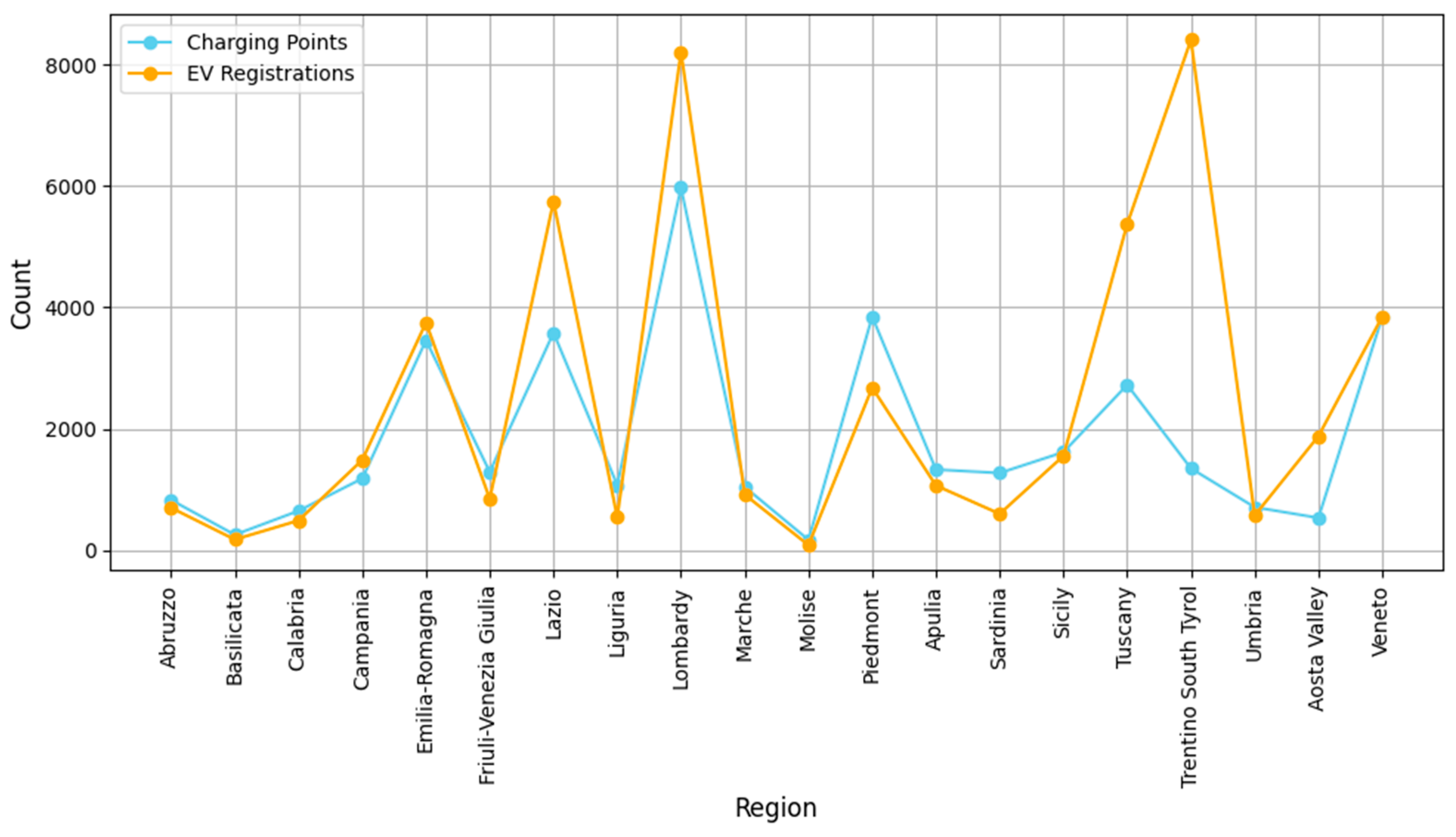
Cluster 4 is composed of four regions, namely Piedmont, Emilia Romagna, Tuscany, and Veneto. All these regions share rather high values of car dependency in the home-to-work trip as well as high values of the number of charging points. As shown in Figure 12 below, the charging point values are not coupled by the same high values as for BEV registrations, meaning that there is a difference in the relative ratios of BEVs/charging points in the regions. This theme could be influenced by a set of factors, from political intentions to financial reasons.

Cluster 3 comprises Aosta Valley and Trentino-South Tyrol, which were highlighted in the beginning as having Special Status. Considering the Special Status, it is worth mentioning that the increased autonomy and deliberative power given to these regions could have improved the centralized decisional power, aiding the adoption of BEVs and distinguishing them from other similar regions. As an example, both these regions are in the top four in terms of GDP per capita, meaning that to a wealthy population with strong purchasing power, the highest regional incentives available are also coupled. When it comes to the proposed analysis, they fit the description given for PC2, meaning that they are rather wealthy and part of low-density zones, for which they find the strongest expression in the dataset. Although specific research should be conducted on merit, it is reasonable to assume such values come from the combination of the financial factors highlighted, coupled with leading positions in sustainability and electric transition. In this context, it is worth highlighting how the interfacing of these regions with countries such as Switzerland, France, and Austria could be playing a role in the adoption of BEVs.

Coming now to the one-point clusters, Liguria—Cluster 0—is of interest since it shows how the uptake of BEVs is not a vertical theme, but rather a horizontal one. In depth, when considering “% of travelers that drive a car while going to work”, Liguria shows the lowest value across the dataset, reaching 49.6% of the respondents. Analyzing only the variable “Electric Vehicle Registrations” would not have shown the role that the mode used in day-to-day life plays in BEV adoption. By further analyzing the ISTAT dataset related to mode repartition, Liguria presents an outstanding percentage of the population that uses private mopeds, reaching 17.7%. Actions that target the scrapping of an old car in favor of a new one are missing a substantial part of the population, effectively reducing the positive effects of such programs.

Campania—Cluster 5—presents an extremely low value for PC2, which is generated by particularly low values of “% of existing vehicles with less than 5 years” and “Median Household income” and particularly high values for both population density variables. The value of PC1 is influenced positively by population density variables and negatively by the actual uptake of EVs and the number of charging points. The combination of the three Principal Components isolates Campania without creating excessive values for PC1 and PC3, so the interpretation of such a position should be associated with the peculiarity of PC2. Interestingly, the value for PC1 suffers from the composition of the factor loadings, since in this case, the PCA is not able to distinguish combinations of a high number of charging points and electric vehicle registrations from high values of population density and population density in the region’s capital. However, confronting this information with Figure 13, it is reasonable to assume that Campania could find a large expression in PC1 if increases in registered income or share of new vehicles take place, and that such increases would reflect back onto electric vehicle registrations.

Lazio—Cluster 2—and Lombardy—Cluster 6—present the highest values for PC1, due to the combination of high values for EV registrations, charging points, and home loan installment. The differences lie in:

• The value of PC3, related to “Number of Charging Points” and “% of travelers that drive a car while going to work”.
• The value of “Density in the Region’s Capital”, which for Lombardy is more than thrice the value for Lazio.

In general, Lombardy is in first position for GDP, accounting for 22% of Italy’s GDP, followed by Lazio, accounting for 11%, a parameter that has surely played a role in opening the way to the adoption of electric vehicles. In addition to this, Lombardy is widely recognized as a dynamic and progressive region, being capable of attracting and retaining foreign talent as well as major global companies in the tech and finance sectors.

Lazio, on the other hand, is inhabited by half the size of Lombardy’s population, and from this point of view, the ratio of BEV registration to population is comparable to that of Lombardy.

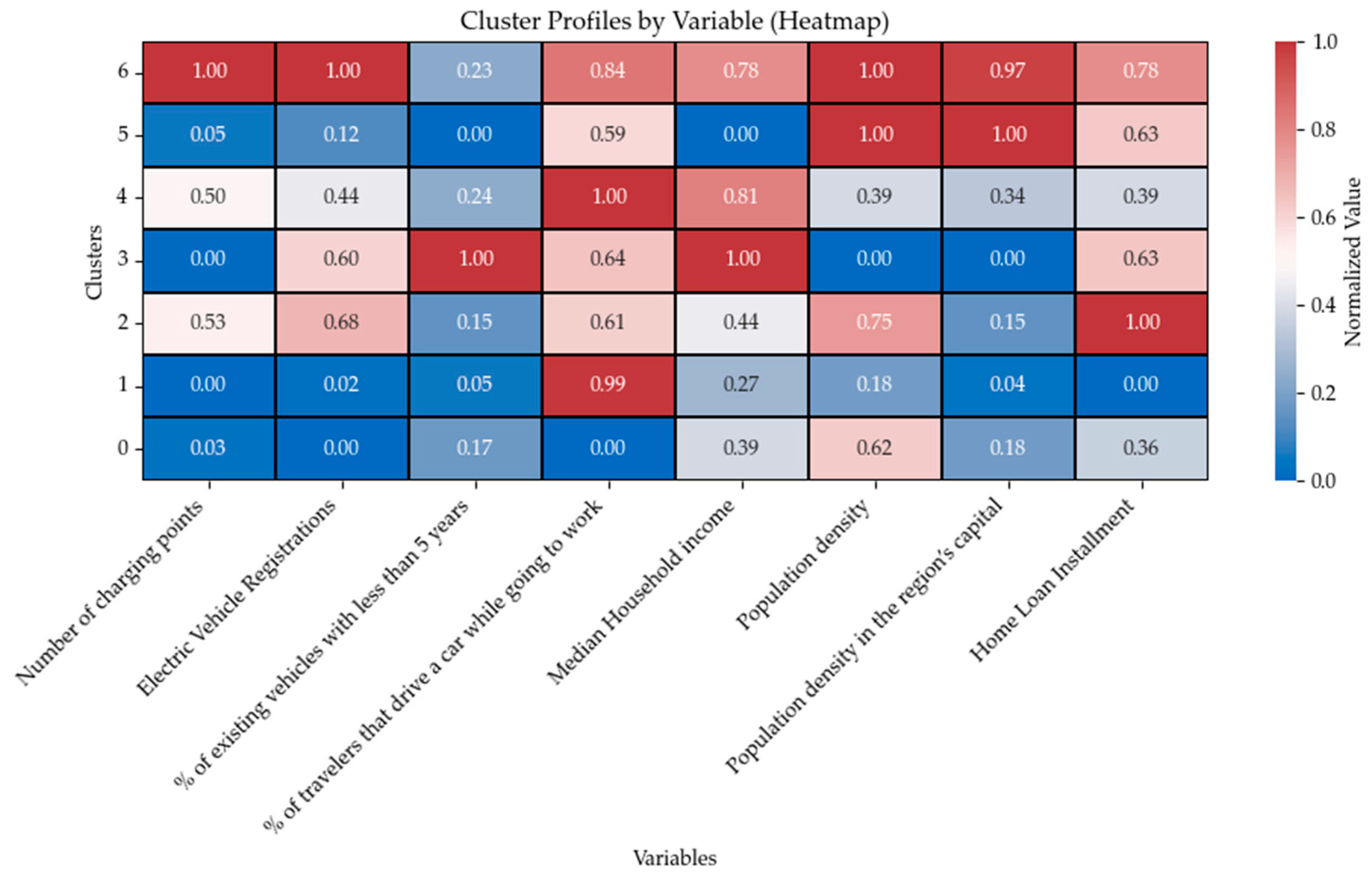
For completeness, a summary of the relationship between the clusters and the starting variables can be seen in Figure 13.

As is possible to see above, most of the clusters are identified by a particularly high value in one of the variables, with exceptions made for Cluster 0 (Liguria) and Cluster 1, which are instead representative of rather low values for most variables, with the latter also presenting, as mentioned, strong car dependence. On the opposite side of the spectrum, Lombardy presents outstandingly high values for most variables, with the exception made for the variables related to vehicle age.

3.1. Policy Recommendations

Considering the results obtained from the previous section, specific recommendations can be made for various regions, following examples suggested in [29]. In Italy, most regions (Cluster 1) seem to be at a similar advancement in terms of the combination of the number of charging points and registration of electric vehicles. For these regions, investments from the public in the charging infrastructure could be coupled with specific incentives towards electric vehicles, possibly envisioning a loan scheme that is already affecting households, such as covering extra costs deriving from a non-zero annual percentage rate and nominal annual interest rate, two parameters that influence the ratio of nominal cost and actual cost of financing the BEV. For cases in which low median income is present, special charging costs could be applied to public charging to ease the energy provision. Some regions benefit from high values of income and frequent changing of vehicles, such as Trentino-South Tyrol and Aosta Valley, although they may suffer on the economic side from having a low population density both throughout the region and in the capital. This finding suggests that the adoption of BEVs is structured and possibly does not need additional incentives. In certain cases, such as Liguria, incentives that not only involve the scrapping of old cars could be needed to reflect the different composition of users. The possibility of considering ownership of scooters could then be investigated, with the possibility of carrying out a parallel process for electric mopeds. In Campania, due to the high population density, the social aspect of EVs could be a focal point to work on, possibly with the intention of transmitting to the wider population the positive aspects of owning an EV. In this regard, possible additional research could be conducted to investigate the perceived barriers to adoption and regional incentives on the estimated WTP. Alternatively, other options such as public awareness advertising or campaigns could be studied. Finally, Lombardy appears to offer the most favorable conditions for adoption, owing to its high population density—both in the region as a whole and in its capital—as well as its above-average median income. While car dependency for commuting is close to the national average and the percentage of vehicles under five years old is relatively high, loan installments remain substantial. Therefore, to support Lombardy’s potential leading role in adoption, the implementation of loan incentives should be encouraged. The introduction of a stricter Limited Traffic Zone (LTZ), reducing it to below 49.5 g/km of CO₂, could be an option to mimic the expected legislation of 2030, which should be supported by additional studies on the response capabilities of the population and successive possible regional incentives.

Generalizing what is suggested up to now, specific studies should be conducted on the capabilities and WTP of the population for each region, possibly coupling such positive actions with restrictive ones such as LTZ, or tariffs such as congestion charges or pollution charges.

3.2. Model Limitations

One of the main limitations of this study is endogenous to the objective pursued: PCA is a statistical analysis, and it is arguable that the sample size (20—one for each region) is comparable, although still larger, to the number of variables chosen (8). Although different metrics have been used for evaluating the process, this factor could still be affecting the results. It is worth noting that the selection of variables was a guided process, but not necessarily a fixed one. The same approach, applied to other countries with different variable distributions, could generate other TEVR, meaning that less (or perhaps more) variance could be captured by the same set of variables. In addition to this, the clustering itself is only intended as an aid to the analysis and visualization, since many clustering options are available, and tweaks in parameters and algorithm selection will produce different results. Examples of this can be found in the possibility of splitting Cluster 0 into multiple clusters, only due to the non-comparable distance between the extremes of the cloud and other single-point or low-point clusters. In the end, the recommendation would be to adapt the choice to follow the guiding principles illustrated in this study, effectively negotiating a solution able to balance the mathematical constraints and the results. An example of this could be to include other social variables, such as commitment to sustainability, in case reliable data on the topic were found, and consequently re-analyze the PC composition and the number of clusters to be chosen.

Due to the structure of the factor loadings, the variables that find a strong expression in PC1, such as the number of charging points, electric vehicle registration, and home loan installment, are the ones that will affect the representation the most, meaning that there is a strong dependence on variations or errors in the data. Additional attention should then be given to collecting and preprocessing such variables.

On a positive note, the objective of the research, as well as the methods used, is not to involve predictions, but rather to offer a statistical description of the case study. From this point of view, the descriptive process could be applied to another country with a comparable or better sample size, as far as a contextual analysis is concerned. It is then not suggested to employ this research as a means of prediction.

For various reasons, mainly data collection and reliability of the sources, it has not been possible to apply the same research approach to provinces, which would raise the sample size to around 100, eliminating this issue. Some of the possible additions to this research could be to:

(1)

Replicate the analysis in a different country;

(2)

Replicate the analysis at a lower administrative level, such as provinces or single cities;

(3)

Replicate the analysis for a different year, such as 2023. In this case, an analysis of coherence between different time data should be conducted, and the variables selected should be fully available across the whole time horizon.

When replicating such results in other countries, all the limitations addressed in this paper should be approached. As an example, when comparing the results with this research, one should expect that the influence of being a border region, such as in the cases of Trentino-South Tyrol and Aosta Valley, could be lower than reported in this work, possibly due to the Special Status mentioned. The nature of the sources, ISTAT and ACI, being national entities, creates strong dependence on the elaboration and collection processes, which means that to ensure scalability of the analysis, data should be obtained from international entities (such as Eurostat, EEA, or OECD), or envision mandatory adaptation and preprocessing of the various sources. In particular, other countries might not have the same data elaboration institutes, and the analysis might then simply not be replicable with the same variables or intentions. Scalability will then only be possible for common variables, under the condition that all data elaboration methods (aggregation, preprocessing, anomaly detection, missing value replacement, etc.) are equal or at least comparable. A simple example of a possible complication of the analysis is selecting data pertaining to the housing market, for which various prices, rates, or profitability might generate different aggregations and KPIs of the state of the market, and consequently of the regions. Another possibility is that, due to the geography of the Italian territory, being fully surrounded by either sea or mountains that act as natural barriers, the results could be different, and possibly even provide a better representation.

4. Conclusions

Electric vehicles’ adoption is a complex topic, with great variability in the distributions of the variables analyzed. Due to the presence of a limited number of regions coupled with the related data, most analyses are not easy to carry out. When these two topics are coupled, predictive tools, especially linear ones, lose power and thus interest. The employment of statistical descriptions such as PCA and Clustering can offer valuable insight into the state of the art of electric vehicle uptake. Thanks to modeling, eight variables have been identified to represent the context of the 20 regions in Italy, and are reduced to three PCs, retaining 83.7% of the variance. Disparities have been studied by means of clustering and data analysis, and addressed by referring to the territories’ characteristics and the financial condition of households. Thanks to its scalability, the analysis opens the possibility of replication in different countries and administrative levels, and shows an innovative method of studying the relative positions of peers in the context of BEV adoption.