Multi-Energy Optimal Dispatching of Port Microgrids Taking into Account the Uncertainty of Photovoltaic Power

Abstract

To tackle the problems of high scheduling costs and low photovoltaic (PV) accommodation rates in port microgrids, which are caused by the coupling of uncertainties in new energy output and load randomness, this paper proposes an optimized scheduling method that integrates scenario analysis with multi-energy complementarity. Firstly, based on the improved Iterative Self-organizing Data Analysis Techniques Algorithm (ISODATA) clustering algorithm and backward reduction method, a set of typical scenarios that represent the uncertainties of PV and load is generated. Secondly, a multi-energy complementary system model is constructed, which includes thermal power, PV, energy storage, electric vehicle (EV) clusters, and demand response. Then, a planning model centered on economy is established. Through multi-energy coordinated optimization, supply–demand balance and cost control are achieved. The simulation results based on the port microgrid of the LEKKI Port in Nigeria show that the proposed method can significantly reduce system operating costs by 18% and improve the PV accommodation rate through energy storage time-shifting, flexible EV scheduling, and demand response incentives. The research findings provide theoretical and technical support for the low-carbon transformation of energy systems in high-volatility load scenarios, such as ports.

1. Introduction

Ports, as global logistics hubs, are typical scenarios with high energy consumption and high emissions. According to statistics, the energy consumption of global ports accounts for 30–40% of the total energy consumption of the maritime transport industry [1]. The load demands of ship shore power, loading and unloading equipment, and cold chain logistics in ports exhibit significant randomness and volatility. Taking the LEKKI Port in Nigeria as an example, due to the irregular arrival times of ships, the peak-valley load difference during the day can reach up to 3500 kW. The traditional scheduling mode mainly relying on thermal power faces economic problems, such as frequent start-stop of generating units and a sharp increase in fuel costs [2]. At the same time, the large-scale application of PV in the LEKKI Port is restricted by the uncertainty of its output. The PV curtailment rate has remained above 15% for a long time, severely restricting the utilization rate of clean energy [3].

In this context, the multi-energy complementary system has become the core approach for the energy transition of ports. The introduction of flexible resources, such as energy storage, electric vehicle (EV), and demand response, can smooth fluctuations through spatiotemporal energy transfer and load regulation [4]. However, multi-energy coordinated scheduling faces two major bottlenecks: the coupling problem of uncertainties brought by the randomness of new energy output and port load, and the challenge of dynamic multi-energy coordination. Therefore, constructing a multi-energy complementary optimal scheduling model for ports that takes into account the uncertainty of new energy is of urgent practical significance for reducing port carbon emissions, improving the PV accommodation rate, and ensuring the economical operation of the multi-energy system [5].

Most existing studies focus on constructing energy scheduling models around economic and environmental goals. References [6,7] establish scheduling models based on fuel costs or PV curtailment penalties according to the output characteristics of single-energy sources, such as thermal power and PV. Reference [8] proposes a strategy to minimize start-stop costs but does not consider the multi-energy complementary requirements under the penetration of new energy. Reference [9] designs an energy storage scheduling model with the PV accommodation rate as a constraint but ignores the synergistic potential of load-side resources. References [10,11,12] study the integration of 2–3 types of energy, such as the “PV-energy storage” or “thermal power-demand response” combinations, and propose a day-ahead optimization model for the PV-energy storage joint system. This model smooths the fluctuations of PV through the charging and discharging of energy storage but does not involve high-randomness loads in port scenarios. Reference [13] introduces demand response to optimize the peak-valley difference, but the model assumes that the charging and discharging behaviors of EVs are completely controllable and does not take into account the power step problem caused by dynamic grid connection and disconnection.

Regarding the uncertainties of new energy and load, mainstream methods include probability modeling and scenario generation techniques. Traditional sampling methods are mainly Monte Carlo simulation, which is widely used to generate random scenarios [14,15], but its computational complexity is high. Latin hypercube sampling (LHS) improves efficiency through stratified sampling [16]. Reference [17] generates 1000 sets of PV scenarios based on LHS, but the scenario redundancy is relatively high. The K-means algorithm is often used for scenario reduction due to its simplicity and efficiency. However, its assumption of a fixed number of clusters and poor adaptability to non-convex data lead to insufficient coverage of typical scenarios [18,19]. Reference [20] uses an improved ISODATA algorithm to optimize the clustering quality through dynamic splitting and merging operations.

The dynamic load in port scenarios and the demand for multi-energy complementarity have gradually attracted attention, yet the research depth remains insufficient. References [21,22] focus on the capacity planning of PV and energy storage in ports. They design the “source-storage” capacity ratio based on static load curves but fail to integrate flexible resources, such as EVs and demand response. Reference [23] proposes a stochastic modeling method for ship shore power load, using the Poisson distribution to simulate the arrival time of ships. However, this model is not coupled with multi-energy scheduling objectives. Reference [24] attempts to treat EV clusters as virtual batteries (VBs), but it overlooks the grid connection and disconnection behaviors of EVs.

The research in this paper provides theoretical support and practical pathways for addressing the key challenges in the low-carbon transformation of port energy systems. The energy scheduling model constructed for the special microgrid scenarios in ports encompasses multiple types of resources, including thermal power, PV, EVs, and energy storage. Based on a progressive framework of scenario generation, reduction, and optimization, it breaks through the limitations of traditional deterministic scheduling models. This significantly reduces the dimensional impact of uncertainties on the optimization model and offers an efficient modeling tool for stochastic optimization under high-penetration new energy scenarios. The main contributions are as follows:

(1)

Modeling of port multi-energy complementary systems: A port microgrid energy structure is constructed, covering PV, thermal power, energy storage, EV clusters, demand response, and interactions with the distribution network. A refined operation model is established.

(2)

Virtual battery model for EV clusters: By introducing an electricity correction term and power-energy coupling constraints, the dynamic grid connection and disconnection behaviors of EVs are characterized to support flexible scheduling.

(3)

Multi-objective optimal scheduling model: With the minimization of total operation costs as the core, a two-stage stochastic programming model is constructed. In the first stage, typical scenarios are generated, and in the second stage, the multi-energy coordinated output is optimized. Through the power purchase–sale balance constraint and multi-energy complementarity strategies, both economic efficiency and the accommodation of clean energy are enhanced.

This paper follows the logical mainline of “problem analysis-model construction-scenario generation-optimization solving-empirical verification”. In Section 2, the port multi-energy complementary system model is constructed, describing the mathematical representations of thermal power units, energy storage stations, EV clusters, and demand response. Section 3 focuses on the generation and reduction of uncertainty scenarios, extracting typical scenarios to provide probabilistic inputs for subsequent optimizations. Section 4 establishes the multi-objective optimal scheduling model and designs a mixed-integer programming model that includes multi-energy complementarity constraints, power purchase-sale balance, and equipment operation boundaries. In Section 5, the model is verified using the microgrid of the LEKKI Port as a case study.

2. Introduction to System Energy Structure and Model Establishment

2.1. Energy Structure of Multi-Energy Complementary Systems

The research subject of this article is the LEKKI Port located in Nigeria. As a coastal port with self-generated power capacity, the main power supply planning for the LEKKI Port includes diesel generator sets at the port, PV power, and the Nigerian power grid. The main electrical equipment includes quay cranes at the port, terminal transport vehicles, cold storage warehouses for storage, and daily power consumption in office areas.

The multi-energy complementary system constructed in this paper integrates five types of energy resources, namely PV, thermal power, energy storage, EVs, and power purchase from the distribution network. Meanwhile, it also incorporates the demand response resources on the load side and the energy models were given according to their respective operational characteristics. Renewable energy is significantly affected by factors, such as time and climate, exhibiting notable uncertainty and intermittency [25]. Additionally, due to the particularity of ports, the arrival time of ships at the dock is irregular, and the daily electricity consumption plan changes greatly. These reasons may lead to problems, such as reduced energy utilization efficiency, decreased system operation stability, and increased scheduling costs.

In conclusion, the energy structure of the multi-energy complementary system in this paper is shown in Figure 1.

To address the above challenges, this study focuses on two indicators: the electricity cost of ports and the PV accommodation rate. Meanwhile, in order to consider the engineering applicability, the calculation time of the method should also be taken into account. By leveraging the complementarity of the five types of power sources in terms of output characteristics and operation modes, the overall benefits are enhanced. Considering that the demand response resources on the user side have become a crucial approach to enhancing the flexibility of the power system, demand response is implemented. By providing policy incentives, users are encouraged to participate in system scheduling, thereby optimizing the electricity load.

2.2. Port Load Characteristics

Based on the statistical analysis of routine monitoring data, as shown in Figure 2, influenced by the randomness of the arrival times of international cargo ships, the peak-valley load difference during the day at the port can reach up to 3500 kW.

Moreover, due to the connection of ships to shore power, the load within each time period also exhibits a high degree of uncertainty. Consequently, even if the next-day load plan and PV power generation forecast can be obtained from the port dispatching department, the influence of uncertainties still needs to be taken into account. In Section 3 of this paper, scenario analysis is conducted for both of them simultaneously.

2.3. Generator Set Model

Considering the impacts of a high proportion of PV power and the uncertainty of ship arrivals at the port, the generator units may face frequently changing operating conditions. Against this background, an operating cost model for thermal power units is established, which includes generation costs and start-stop costs. Since this paper focuses on hourly level scheduling, the time unit for each operating period is one hour, and the ramping cost can be neglected. The cost function is as follows:

(1)

Fuel cost:

The cost function of a single generator is

$$C_{\mathrm{G}i}\left(t\right)=\left[a_i{P}_{\mathrm{G},i,t}^2+b_i{P}_{\mathrm{G},i,t}+c_i\right]\mathsf{\Delta }t$$

(1)

where C_Gi(t) represents the fuel cost of the i-th generator, P_G,i,t denotes the output value of the i-th generator at time t, and a_i, b_i, c_i are the fuel cost characteristic parameters of the i-th generator [26]. ∆t is the scheduling step size, and its value is 1 h.

Therefore, the cost function of a generator set composed of multiple generators is

$$C_{\mathrm{GE}}\left(t\right)={\displaystyle \sum _{t=1}^T{\displaystyle \sum _{i=1}^N{u}_{i,t}}}{C}_{\mathrm{G}i}\left(t\right)$$

(2)

where C_GE(t) represents the fuel cost of a generator set composed of N generators within the operating time T, and u_i,t denotes the start-stop status of the i-th generator at time t. A value of 0 indicates the shutdown state, and a value of 1 represents the startup state.

(2)

Start-stop cost:

During the start-up and shut-down processes of a generator set, additional mechanical wear and thermal stress may occur, which can lead to costs, such as part replacement and maintenance. Considering the start-stop of the generator set in actual scheduling and reasonably arranging the output plan of the generator set can effectively reduce the comprehensive cost. The calculation formula for the start-stop cost is as follows

$$C_{\mathrm{GS}}\left(t\right)={\displaystyle \sum _{t=1}^T{\displaystyle \sum _{i=1}^N\left[u_{i,t}\left(1-u_{i,t-1}\right)S_{\mathrm{G},i}\right]}}\mathsf{\Delta }t$$

(3)

where C_GS (t) represents the start-stop cost of the generator set, and S_G,i denotes the start-stop cost of the i-th generator.

In conclusion, the operating cost C_G(t) of the generator set is

$$C_{\mathrm{G}}\left(t\right)=C_{\mathrm{GE}}\left(t\right)+C_{\mathrm{GS}}\left(t\right)$$

(4)

2.4. Electrochemical Energy Storage Model

The operating cost of energy storage mainly considers its initial investment cost and operation-maintenance cost. The average charging and discharging cost C_S(t) of the port’s energy storage power station within the investment payback period t can be expressed as follows:

$$C_{\mathrm{S}}\left(t\right)={\displaystyle \sum _{t=1}^T{K}_{\mathrm{S}}\left[P_{\mathrm{S},t}^{\mathrm{dis}}/\eta +P_{\mathrm{S},t}^{\mathrm{ch}}\eta \right]}\mathsf{\Delta }t$$

(5)

In the formula, K_s represents the unit charging and discharging cost after conversion; $P_{\mathrm{S},t}^{\mathrm{dis}}$ and $P_{\mathrm{S},t}^{\mathrm{ch}}$, respectively, denote the discharge power/output power of the energy storage inverter on the AC side during time period t. η is the charging and discharging efficiency of the energy storage unit.

2.5. EV Model

(1)

Single EV Model

Different from electrochemical energy storage, the usage demands and schedules of port workers need to be taken into account for EVs. Compared with the EV cluster as a whole, each EV may experience grid connection and disconnection behaviors at any time. Therefore, the research on EVs is carried out from two perspectives: single EV and EV cluster.

The feasible region model of a typical single EV under different scenarios is shown in Figure 3.

The energy ranges corresponding to Figure 3 are given by Equations (6) and (7):

$$E_{i,t}^{\mathrm{ev},\max }=\min \left[\left(E_{i,T_0}+{\displaystyle \sum _{t=T_0}^{T_{\mathrm{d}}}{P}_{i,t}^{\max }\mathsf{\Delta }t}\right),E_i^{\max }\right]\hspace{1em}t\in \left(T_0,T_d\right)$$

(6)

$$E_{i,t}^{\mathrm{ev},\min }=\max \left[\left(E_{i,T_0}+{\displaystyle \sum _{t=T_0}^{T_{\mathrm{d}}}{P}_{i,t}^{\min }\mathsf{\Delta }t}\right),E_i^{\min }\right]\hspace{1em}t\in \left(T_0,T_d\right)$$

(7)

In the formula: $E_{i,t}^{\mathrm{ev},\max }$ and $E_{i,t}^{\mathrm{ev},\min }$ represent the maximum and minimum battery levels of the i-th EV during time period t, as well as the battery level expected by the owner when the EV is offline; T₀ and T_d are the times when the EV connects to and disconnects from the grid, respectively; $E_{i,T_0}$ is the initial battery level of the i-th EV at time T₀; $P_i^{\max }$ and $P_i^{\min }$ are the theoretical maximum and minimum charging power of the i-th EV. When their values are negative, it indicates the discharging state; $E_i^{\max }$ and $E_i^{\min }$ are the theoretical maximum and minimum battery levels of the i-th EV; E_ex is the battery level expected by the owner when the EV disconnects from the grid.

Therefore, considering the influence of the EV’s energy range, the upper and lower limits of power are as follows:

$$P_{i,t}^{\mathrm{ev},\max }=\min \left[\left(E_{i,t+1}^{\mathrm{ev},\max }-E_{i,t}^{\mathrm{ev},\min }\right)/\mathsf{\Delta }t,P_{i,t}^{\max }\right]\hspace{1em}t\in \left(T_0,T_d-1\right)$$

(8)

$$P_{i,t}^{\mathrm{ev},\min }=\max \left[\left(E_{i,t+1}^{\mathrm{ev},\min }-E_{i,t}^{\mathrm{ev},\max }\right)/\mathsf{\Delta }t,P_{i,t}^{\min }\right]\hspace{1em}t\in \left(T_0,T_d-1\right)$$

(9)

In the formula: $P_{i,t}^{\mathrm{ev},\max }$ and $P_{i,t}^{\mathrm{ev},\min }$, respectively, represent the upper and lower bounds of the actual power of the i-th EV during time period t; T_d−1 is the moment immediately before the EV disconnects from the grid. $E_{i,t+1}^{\mathrm{ev},\max }$ and $E_{i,t+1}^{\mathrm{ev},\min }$ are the lower and upper bounds of the battery level of the i-th EV calculated for time period t + 1.

Based on the above descriptions of the boundaries of power and energy, the state constraints of a single EV are as follows:

$$P_{i,t}^{\mathrm{ev},\min }\le P_{i,t}^{\mathrm{ev}}\le P_{i,t}^{\mathrm{ev},\max }$$

(10)

$$E_{i,t}^{\mathrm{ev},\min }\le E_{i,t}^{\mathrm{ev}}\le E_{i,t}^{\mathrm{ev},\max }$$

(11)

$$E_{i,t+1}^{\mathrm{ev}}=E_{i,t}^{\mathrm{ev}}+P_{i,t}^{\mathrm{ev}}\mathsf{\Delta }t$$

(12)

In the formula, $P_{i,t}^{\mathrm{ev}}$ represents the actual power of the i-th EV during time period t; $E_{i,t}^{\mathrm{ev}}$ and $E_{i,t+1}^{\mathrm{ev}}$ represent the energy of the i-th EV during time periods t and t + 1, respectively.

(2)

Cluster EV model

EVs share similar characteristics with energy storage batteries. Therefore, a virtual battery model is employed to quantitatively describe the clustered EVs formed by multiple EVs, that is, battery parameters are used to describe the clustered EVs. Based on various constraints, the cumulative boundaries under extreme scenarios are obtained as follows:

$$E_t^{\mathrm{VB},\max }={\displaystyle \sum _{i=1}^{N_{\mathrm{ev}}}{E}_{i,t}^{\mathrm{ev},\max }}$$

(13)

$$E_t^{\mathrm{VB},\min }={\displaystyle \sum _{i=1}^{N_{\mathrm{ev}}}{E}_{i,t}^{\mathrm{ev},\min }}$$

(14)

$$P_t^{\mathrm{VB},\max }={\displaystyle \sum _{i=1}^{N_{\mathrm{ev}}}{P}_{i,t}^{\mathrm{ev},\max }}$$

(15)

$$P_t^{\mathrm{VB},\min }={\displaystyle \sum _{i=1}^{N_{\mathrm{ev}}}{P}_{i,t}^{\mathrm{ev},\min }}$$

(16)

In the formula: $E_t^{\mathrm{VB},\max }$ and $E_t^{\mathrm{VB},\min }$, respectively, represent the upper and lower bounds of the battery level of the EV cluster during time period t; $P_t^{\mathrm{VB},\max }$ and $P_t^{\mathrm{VB},\min }$, respectively, represent the upper and lower bounds of the power of the EV cluster during time period t; N_ev is the number of EVs within the cluster.

Different from energy storage stations, individual EVs in the EV cluster may experience uncertain grid connection and disconnection due to work schedules, thereby causing power step-change phenomena. Consequently, the integrated power fails to achieve the time-axis coupling of the integrated energy. Taking the influence of the i-th EV on the virtual battery model of the EV cluster as an example, it is illustrated in Figure 4.

Among them, EV_i represents the i-th EV in the cluster. Initially, EV_i is in the driving state. When it enters the grid connection period, the electrical energy of the VB model of the EV cluster will suddenly increase, causing a step-change in the electrical energy of the VB. This process will occur again when it enters the off-grid state. Equation (17) is the correction equation proposed for the VB model to solve the above problems:

$$E_{t+1}^{\mathrm{VB},r}={\displaystyle \sum _{i=1}^{N_{\mathrm{ev}}}{E}_{i,t+1}^{\mathrm{ev},\max }\left(W_{i,t+1}^2-W_{i,t}^2\right)}$$

(17)

In the formula, $E_{t+1}^{\mathrm{VB},r}$ represents the change in battery level caused by the grid connection and disconnection of an EV; W_i,t+1 and W_i,t represent the grid connection status of the i-th EV at time t + 1 and time t, respectively, with a value of 0 indicating the driving state or a value of 1 indicating the grid connected state. Based on the obtained boundaries of power and energy of the EV cluster, the VB model of the EV cluster is as follows.

$$P_t^{\mathrm{VB},\min }\le P_t^{\mathrm{VB}}\le P_t^{\mathrm{VB},\max }$$

(18)

$$E_t^{\mathrm{VB},\min }\le E_t^{\mathrm{VB}}\le E_t^{\mathrm{VB},\max }$$

(19)

$$E_{t+1}^{\mathrm{VB}}=E_t^{\mathrm{VB}}+P_t^{\mathrm{VB}}\mathsf{\Delta }t+E_{t+1}^{\mathrm{VB},r}$$

(20)

In the formula: $P_t^{\mathrm{VB}}$ represents the integrated power of the EV cluster during time period t; $E_t^{\mathrm{VB}}$ represents the integrated energy of the EV cluster during time period t. The VB model can not only accurately describe the charging and discharging flexibility of EVs over multiple time periods, but also effectively reduces the dimensionality of decision variables and improves computational efficiency due to the fact that the decision vector has only one dimension.

2.6. Demand Response Model

Demand response refers to the ability of end-users in the power system to actively reduce or adjust their electricity loads according to market signals or grid dispatch instructions. The electricity consumption characteristics of demand response during the service process can be represented by the following constraints:

$${\displaystyle \sum _{t=1}^{24}{P}_{\mathrm{DR},t}}\mathsf{\Delta }t=D_{\mathrm{DR}}$$

(21)

$$D_{\mathrm{DR},t}^{\min }\le P_{\mathrm{DR},t}\le D_{\mathrm{DR},t}^{\max }$$

(22)

In the formula, P_DR(t) represents the actual dispatch power of the microgrid for the demand-response load during time period t; D_DR represents the total electricity demand of the demand-response load within a day, and the port statistical data shows it is 4500 kW·h; $D_{\mathrm{DR},t}^{\min }$ and $D_{\mathrm{DR},t}^{\max }$ represent the maximum and minimum electricity demands of the demand-response load during time period t, respectively, which are related to the users’ restrictions.

On the basis of meeting the above constraints, the microgrid can flexibly adjust the electricity consumption plan of the demand-response load. However, the change in the electricity consumption plan will inevitably affect the users’ plans. Therefore, the microgrid needs to provide economic compensation. The dispatch cost C_DR(t) required within time T can be expressed as follows:

$$C_{\mathrm{DR}}\left(t\right)=K_{\mathrm{DR}}{\displaystyle \sum _{t=1}^T\left|P_{\mathrm{DR},t}-P_{\mathrm{DR},t}^{*}\right|}$$

(23)

In the formula, K_DR represents the unit dispatch cost of the demand-response load; $P_{\mathrm{DR},t}^{*}$ represents the expected electricity power of the demand-response load during time period t. $\left|P_{\mathrm{DR},t}-P_{\mathrm{DR},t}^{*}\right|$ represents the deviation between the actual dispatch power and the expected electricity power.

2.7. Power Purchase and Sale Model

When the power generation part within the microgrid fails to meet the load demand of the port, it is necessary to purchase electricity from the distribution network. Conversely, the microgrid can sell the surplus electricity to the distribution network to obtain profits. The interaction power between the microgrid and the distribution network needs to meet the following balance constraints:

$$P_{\mathrm{M},t}^{\mathrm{buy}}-P_{\mathrm{M},t}^{\mathrm{sell}}=P_{\mathrm{DR},t}+P_{\mathrm{L},t}+P_{\mathrm{S},t}^{\mathrm{ch}}+P_t^{\mathrm{VB}}-\left(P_{\mathrm{G},t}+P_{\mathrm{PV},t}+P_{\mathrm{S},t}^{\mathrm{dis}}\right)$$

(24)

In the formula, $P_{\mathrm{M},t}^{\mathrm{buy}}$ and $P_{\mathrm{M},t}^{\mathrm{sell}}$, respectively, represent the power purchased from and sold to the distribution network by the microgrid during time period t. P_L,t and P_PV,t, respectively, represent the power of conventional loads and the output power of PV within the microgrid during time period t. The interaction power between the microgrid and the distribution network shall meet the following requirements:

$$0\le P_{\mathrm{M},t}^{\mathrm{buy}}\le u_{\mathrm{M},t}{P}_{\mathrm{M}}^{\max }$$

(25)

$$0\le P_{\mathrm{M},t}^{\mathrm{sell}}\le \left[1-u_{\mathrm{M},t}\right]P_{\mathrm{M}}^{\max }$$

(26)

In the formula, $P_{\mathrm{M}}^{\max }$ represents the maximum value of the power exchange between the microgrid and the distribution network. The value of $P_{\mathrm{M}}^{\max }$ needs to take into account factors, such as the capacity of the transformer at the connection point between the distribution network and the microgrid, as well as specific policies. $u_{\mathrm{M},t}$ is the power purchase-sale status of the microgrid with respect to the distribution network. When $u_{\mathrm{M},t}$ = 1, it indicates that the microgrid purchases power from the distribution network; when $u_{\mathrm{M},t}$ = 0, it indicates that the microgrid sells power to the distribution network. The interaction cost C_M(t) between the microgrid and the distribution network can be expressed as follows:

$$C_{\mathrm{M}}\left(t\right)={\displaystyle \sum _{t=1}^T{\lambda }_{\mathrm{M},t}\left[P_{\mathrm{M},t}^{\mathrm{buy}}-P_{\mathrm{M},t}^{\mathrm{sell}}\right]\mathsf{\Delta }t}$$

(27)

In the formula, λ_M,t represents the day-ahead trading price of the distribution network.

3. Scenario Analysis of PV and Load Outputs

The uncertainties mentioned in this article are reflected in the two types of data: PV output power and load power. The approach to handle the uncertainties of these two types of data in this article is that by generating a large number of possible scenarios and then aggregating them into five representative typical scenarios, the uncertainties of PV and load are indirectly reflected through five different scenarios. Therefore, it will not be reflected in other models, but directly incorporated into the optimization problem along with other models for solution. The final five results are precisely the system optimization scheduling results considering the uncertainties. The principles of scenario generation and reduction for PV and load outputs are consistent. The following takes PV as an example for illustration.

3.1. Scenario Generation Based on Latin Hypercube Sampling (LHS)

LHS, a statistical method for designing experiments and sampling parameter spaces, is part of the Latin Hypercube Design. This design can be used to effectively cover multi-dimensional parameter spaces. The basic idea of LHS is to divide the possible range of values for each parameter into equal sub-intervals, and then randomly select a sample point from each sub-interval. In this way, each parameter can be uniformly distributed throughout the parameter space, enabling the effective exploration of multi-dimensional parameter spaces with a smaller sample size and providing better parameter coverage and sampling efficiency.

(1)

Data Pre-processing: Input the original data of the estimated PV power generation for the next day. Divide the day into 24 time periods.

(2)

LHS Sampling: Assume that the dimensionality of the sampling samples is N and the sample length is 24. Generate an N × 24 sample space through LHS. Each dimension of the sample contains 24 data points ranging from 0 to 1.

(3)

Scenario Generation: Utilize the data in step (1) to perform an inverse transformation operation on the 0–1 data of each sample point in the N-dimensional sample space. After the transformation, the corresponding PV output scenarios are obtained.

3.2. Scenario Clustering Based on Improved ISODATA

When the scale of the initial scenario generation set increases, the complexity of the optimization scheduling model also grows. Scenario reduction can select a few typical scenarios from the initial scenario set to simplify the calculation. Currently, most studies use clustering or non-clustering methods for scenario reduction. This paper combines the two types of methods and adopts a way of clustering first and then reducing to achieve scenario reduction.

The traditional K-means clustering algorithm is conceptually straightforward and easy to implement, yet it requires manual determination of the number of clusters. When applied to large-scale scenario sets, its performance exhibits inconsistency depending on the preset initial cluster count. The ISODATA algorithm introduces cluster splitting and merging operations, enabling the dynamic adjustment of cluster numbers based on actual conditions while maintaining a given expected cluster count. However, similar to conventional K-means, ISODATA also suffers from the issue of the random initialization of cluster centers, which may adversely affect clustering convergence. Therefore, this study employs an improved ISODATA algorithm for clustering initial scenario sets. Taking photovoltaic power output scenarios as an example, the specific operational procedures are as follows:

(1)

Input the random PV output scenario set C = {x_i, i = 1, 2, …, N}, and randomly select a single scenario as the initial clustering center z₁.

(2)

Calculate the distances from the remaining scenarios to the determined clustering center z₁, record the shortest distance in each scenario and denote it as d(x_i). Calculate the probability using Equation (28) and select the new round of initial clustering centers according to the probabilities.

$$P_i={\displaystyle \frac{d{\left(x_i\right)}^2}{{\displaystyle \sum _{x\in N}d{\left(x_i\right)}^2}}}$$

(28)

(3)

Repeat step 2 until k initial clustering centers {z₁, z₂, z₃, …. z_k} are selected.

(4)

Calculate the Euclidean distances between each initial clustering center and the random scenarios and assign each scenario to the cluster where the nearest clustering center is located.

(5)

Determine whether the number of scenarios in each cluster meets the condition of Equation (29). If it does, delete this cluster, reallocate the scenarios in this cluster, and update the number of clusters to k = k − 1.

$$S_j<{\theta }_{\mathrm{N}}$$

(29)

In the formula, S_j represents the number of scenarios in the j-th clustering cluster, and θ_N represents the minimum number of scenarios allowed in a clustering cluster.

(1)

Update the clustering center {z_j, j = 1, 2, …, k} by modifying the following formula:

$$S_j<{\theta }_{\mathrm{N}}$$

(30)

(7)

Use Equation (31) to calculate the average distance D_j from scenarios within each cluster to their corresponding clustering centers and use Equation (32) to calculate the average distance D from all scenarios to the clustering centers.

$$D_j={\displaystyle \frac{1}{\left|S_j\right|}}{\displaystyle \sum _{x\in S_j}‖x-z_j‖}$$

(31)

$$D={\displaystyle \frac{1}{\left|S_j\right|}}{\displaystyle \sum _1^{\left|S_j\right|}\left|S_j\right|}{D}_j$$

(32)

(8)

Determine whether to split. Enter step 10 if the following conditions are met:

If the current number of clusters is less than half of the expected number, perform a splitting operation; the current iteration number is an even number or the current number of clusters is not less than twice the expected number; the maximum value σ_max of the standard deviation vector of the distances between scenarios in a certain clustering cluster exceeds the standard deviation threshold.

(9)

Determine whether to merge. Enter step 11 if the following conditions are met:

The current iteration number is an even number or the current number of clusters is not less than twice the expected number; the average inter-cluster distance D is less than the set threshold θ_C.

(10)

Start the splitting operation. Set the splitting parameter l. The clustering centers $z_1^{’}$ and $z_2^{’}$ of the two new clusters formed after splitting can be calculated by the following two formulas:

$$z_1^{’}=z_i+l{\left[0,\dots ,{\sigma }_{\max },\dots ,0\right]}^T,0<l<1$$

(33)

$$z_2^{’}=z_i-l{\left[0,\dots ,{\sigma }_{\max },\dots ,0\right]}^T,0<l<1$$

(34)

(11)

Start the merging operation. The clustering center $z^{’}$ of the new cluster after merging can be expressed by the following formula:

$$z^{’}={\displaystyle \frac{1}{\left|S_i\right|+\left|S_j\right|}}\left(\left|S_i\right|z_i+\left|S_j\right|z_j\right)$$

(35)

(12)

Iterate repeatedly until the clustering results no longer change or the iteration limit is reached.

Through the above process, the typical scenario clusters after clustering can be obtained.

3.3. PV Output Scenario Reduction Based on the Backward Elimination Method

Based on the backward elimination method, a reduction model for the clustering clusters of PV random output scenarios is established. Select the scenario set of a certain cluster as S = {w₁, …, w_i, w_j, …,w_n}, which contains n scenarios. The scenarios to be deleted are discarded into the scenario set S’. The specific steps are as follows:

(1)

Initialization: Set the scenario set S’ as an empty set.

(2)

Start the iteration: Calculate the probability distance of each scenario according to Equation (36).

$${\displaystyle \sum _{i\in S’}{p}_i\min d\left(w_i,w_j\right)}\hspace{1em}j\notin S’$$

(36)

In the formula, p_i represents the probability of the occurrence of scenario w_i; d(w_i,w_j) represents the Euclidean distance between two scenarios.

(3)

Scenario deletion: Select the scenario w_i that minimizes Equation (36) as the discarded scenario and add it to S’. Update the number of scenarios in the original scenario set as n = n−1.

(4)

Scenario replacement: In the updated scenario set S, find the scenario w_j that is closest to the scenario w, and use it to replace the discarded scenario w_i. Update the probability of the scenario as p_j’ = p_j + p_i.

(5)

Return to step 2 until the number of remaining scenarios in the set S reaches the given value and then stop the iteration.

Through the above steps, the typical scenarios after the reduction of each cluster can be obtained. It should be noted that the probabilities calculated during the backward reduction process only represent the probabilities of the typical scenarios occurring in the corresponding clustering set S. These probabilities should be multiplied by the probabilities of their clusters occurring in the initial scenario set to obtain the actual probabilities.

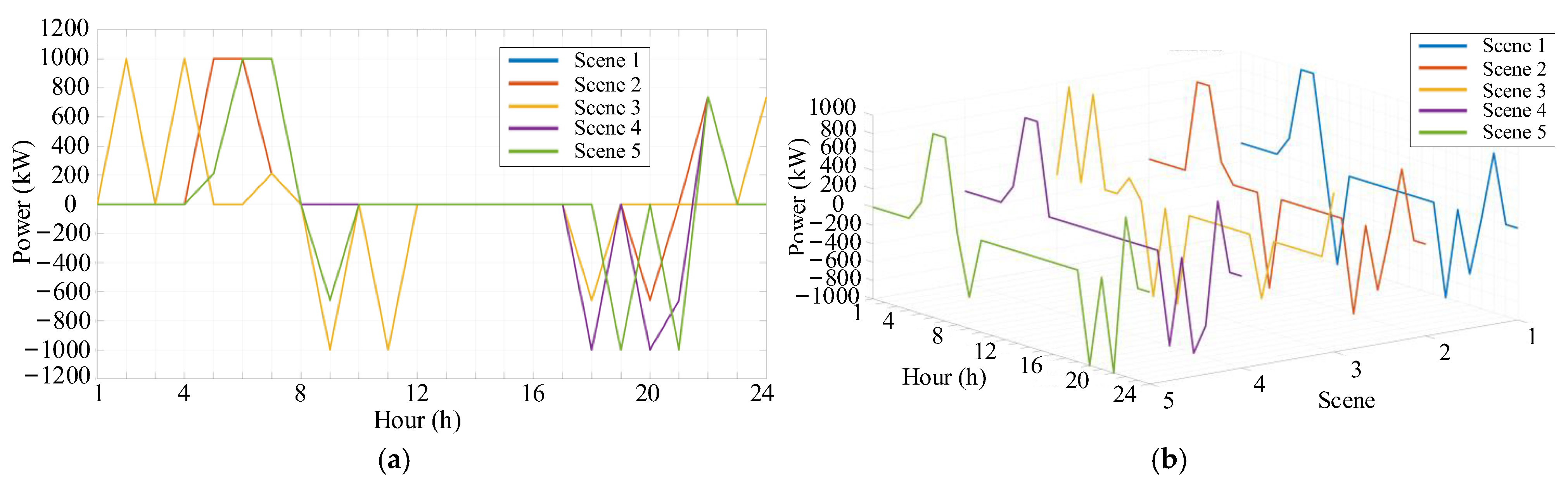
3.4. Scenario Generation Example Analysis

(1)

Scenario Generation Results

In this paper, the measured light and load data of a typical day in March at the port are selected, with a collection interval of 1 h. The initial scenario set is obtained according to the scenario generation method in Section 3.1. The initial number of scenarios is set to 1000. Figure 5 and Figure 6 show the initial scenario sets of load and PV output, respectively.

(2)

Scenario reduction results

The backward elimination method is adopted to retain a set of typical scenarios in each cluster, and ultimately, five typical scenarios are obtained.

Table 1. Probabilities of typical scenarios of load and PV.

Scenario Number	1	2	3	4	5
probability	0.132	0.255	0.197	0.145	0.217

presents the probabilities of each typical scenario. Figure 7 and Figure 8 represent the final reduced scenarios of load and PV output, respectively.

4. Optimization Model of Multi-Energy Complementary System

4.1. Optimization Objectives

The main purpose of this study is to reduce the operating costs f of various equipment in the port, including the operating cost of generator sets C_G, energy storage cost C_S, demand response cost C_DR, and electricity purchase–sale cost C_M. An economic dispatch model that conforms to the low-carbon concept is established with the sum of these costs as the optimization objective. The gurobi solve in Matlab is used to solve the optimization problem:

$$\min f=C_{\mathrm{G}}+C_{\mathrm{S}}+C_{\mathrm{DR}}+C_{\mathrm{M}}$$

(37)

4.2. Constraints

(1)

PV accommodation rate constraint

The PV accommodation rate serves as an evaluation metric, which is expressed as the ratio of the actual connected PV output to the forecasted PV output within the scheduling period. The larger the value, the stronger the system’s accommodation capacity.

$$0\le f_{\mathrm{PV}}={\displaystyle \frac{{\displaystyle \sum _{t=1}^T{P}_{\mathrm{PV},t}}}{{\displaystyle \sum _{t=1}^T{P}_{\mathrm{PV},t}^{’}}}}\le 1$$

(38)

In the formula, f_PV is the PV accommodation rate; $P_{\mathrm{PV},t}$ and $P_{\mathrm{PV},t}^{’}$ are the actual output and the forecasted output of the PV power station, respectively.

(2)

Generator output constraint

$$P_{\mathrm{G},t}^{\min }\le P_{\mathrm{G},i,t}\le P_{\mathrm{G},t}^{\max }$$

(39)

In the formula, $P_{\mathrm{G},t}^{\max }$ and $P_{\mathrm{G},t}^{\min }$ are the upper and lower limits of the output of the i-th generator set, respectively.

(3)

Electrochemical energy storage charge-discharge constraint

$$0\le P_{\mathrm{S},t}^{\mathrm{dis}}\le u_{\mathrm{S},t}{P}_{\mathrm{S}}^{\max }$$

(40)

$$0\le P_{\mathrm{S},t}^{\mathrm{ch}}\le \left[1-u_{\mathrm{S},t}\right]P_{\mathrm{S}}^{\max }$$

(41)

$$\eta {\displaystyle \sum _{t=1}^{24}{P}_{\mathrm{S},t}^{\mathrm{ch}}\mathsf{\Delta }t}-{\displaystyle \frac{1}{\eta }}{\displaystyle \sum _{t=1}^{24}{P}_{\mathrm{S},t}^{\mathrm{dis}}\mathsf{\Delta }t}=0$$

(42)

$$E_{\mathrm{S}}^{\min }\le E_{\mathrm{S}}\left(0\right)+\eta {\displaystyle \sum _{t=1}^T{P}_{\mathrm{S},t}^{\mathrm{ch}}}\mathsf{\Delta }t-{\displaystyle \frac{1}{\eta }}{\displaystyle \sum _{t=1}^T{P}_{\mathrm{S},t}^{\mathrm{dis}}}\mathsf{\Delta }t\le E_{\mathrm{S}}^{\max }$$

(43)

Equations (40) and (41) are the charging and discharging power constraints of the energy storage, respectively. $P_{\mathrm{S}}^{\max }$ is the maximum allowable charging and discharging power of the energy storage, which is mainly limited by the capacity of the grid connected inverter device of the energy storage. $u_{\mathrm{S},t}$ represents the charging and discharging state of the energy storage. When $u_{\mathrm{S},t}$ = 1, it indicates discharging; when $u_{\mathrm{S},t}$ = 0, it indicates charging. Equation (42) ensures that the capacity of the energy storage at the beginning and the end of the scheduling period is equal, which is conducive to the cyclic scheduling of the energy storage. Equation (43) represents the remaining capacity constraint of the energy storage in each time period. E_S(0) is the capacity of the energy storage at the beginning of the scheduling period, and $E_{\mathrm{S}}^{\max }$ and $E_{\mathrm{S}}^{\min }$ are the maximum and minimum allowable remaining capacities of the energy storage during the scheduling process, respectively. The purpose of this constraint is to prevent over-charging or over-discharging of the energy storage and extend the service life of the energy storage.

(4)

Demand response constraint

The operating characteristics of demand response are shown in Equations (21) and (22) in Section 2.6. Here, the constraints considering electricity price are additionally taken into account. The electricity purchase cost of users is the key factor affecting the satisfaction degree of users participating in demand response. Therefore, after the scheduling of demand response, the total electricity purchase cost within a day should not exceed the total electricity purchase cost before scheduling.

$${\displaystyle \sum _{t=1}^{24}{\lambda }_{\mathrm{M},t}{P}_{\mathrm{DR},t}}\mathsf{\Delta }t\le {\displaystyle \sum _{t=1}^{24}{\lambda }_{\mathrm{M},t}{P}_{\mathrm{load},t}}\mathsf{\Delta }t$$

(44)

λ_M,t in the formula represents the electricity price at time t, and $P_{\mathrm{load},t}$ represents the demand-response load value before scheduling at time t.

(5)

Fleet EV constraint

The constraint conditions of the fleet of EVs are similar to those of energy storage, which are shown as Equations (18)–(20).

5. Case Analysis

5.1. Basic System Parameters

A simulation analysis is carried out for the actual micro-grid of the LEKKI Port. A 3.6 MW PV power station, a 1 MW/3.6 MW·h energy storage power station, six electric trucks and tire cranes, and four generator sets are connected to the port. The basic parameters are shown in

Table 2. Basic parameters of generator sets.

Unit	${\mathit{P}}_{\mathbf{G},\mathit{t}}^{\mathbf{max}}$$/{\mathit{P}}_{\mathbf{G},\mathit{t}}^{\mathbf{min}}$	Cost-Characteristic Parameters			SG,i
		${\mathit{a}}_{\mathit{i}}$/(Dollar/MW2)	${\mathit{b}}_{\mathit{i}}$/(Dollar/MW2)	${\mathit{c}}_{\mathit{i}}$/(Dollar/MW2)
1	500/40	0.152	147.21	3400	35,000
2	500/40	0.152	147.21	3700	31,500
3	500/40	0.152	147.21	3450	31,500
4	600/40	0.183	167.44	4660	21,000

,

Table 3. Basic parameters of the demand response.

Parameters	Value
$P_{\mathrm{S}}^{\max }$/kW	1000
η	0.95/0.95
Ks/(dollar/MW2)	0.38
$E_{\mathrm{S}}^{\max }$/kw·h	3600
$E_{\mathrm{S}}^{\min }$/kw·h	800
ES(0)/kw·h	1500

and

Table 4. Basic parameters of the energy storage system.

Parameters	${\mathit{D}}_{\mathbf{DR},\mathit{t}}^{\mathbf{max}}$/kW	${\mathit{D}}_{\mathbf{DR},\mathit{t}}^{\mathbf{min}}$	KDR
Value	400	50	0.22

. The system scheduling period is 24 h with a time interval of 1 h. The initial load data on a typical day, PV prediction data, and EV data are provided by the port operator. We used a randomly selected day of the year but also considered its representativeness. When choosing, we excluded extreme data without special circumstances. This section will apply the five final scenarios generated previously and substitute them into the scheduling model, respectively, to obtain the final optimization results and make comparisons.

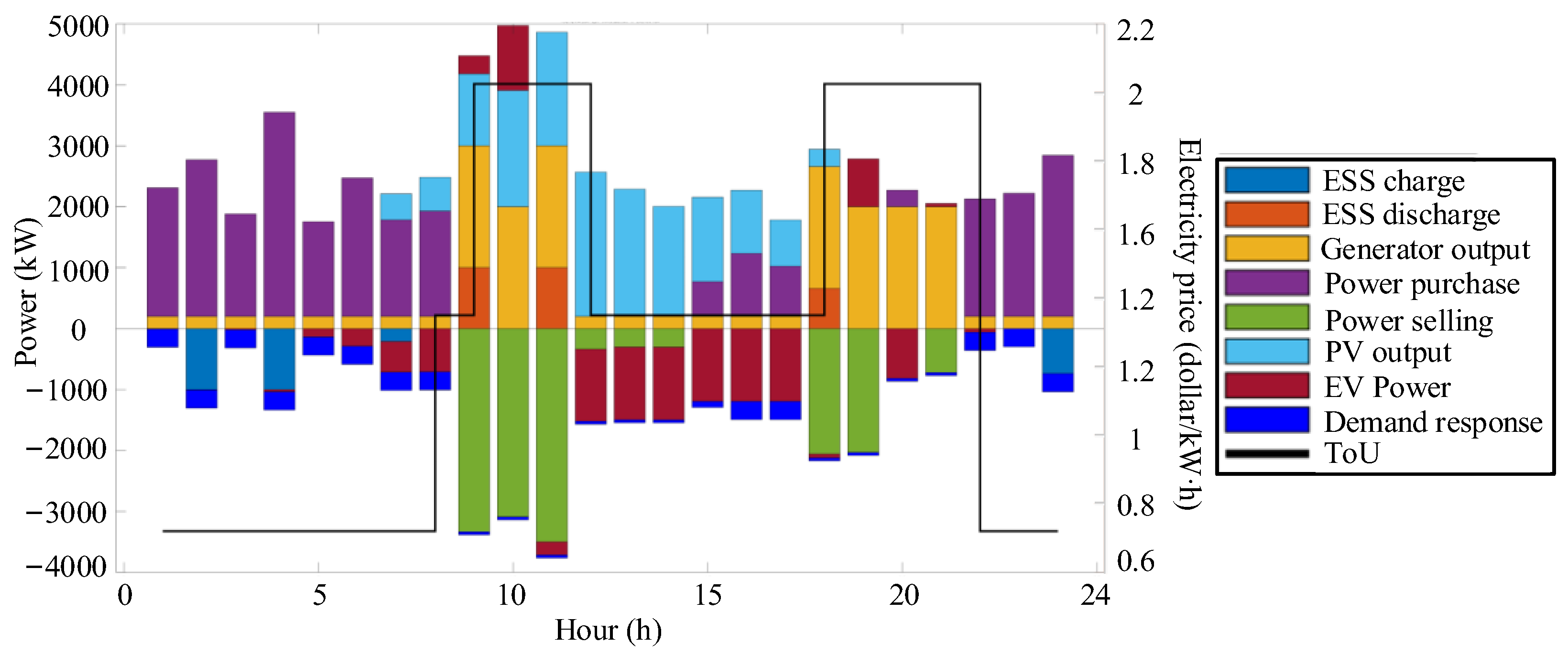
5.2. Energy Balance Results

After the system conducts energy balance through the scheduling model, the average cost is reduced from 23,419.51 to 19,230.11. The average PV accommodation rate is 91.73%, which is an 8% increase compared to the original curtailment rate of over 15%.

Based on the PV forecasted output and load demand on a typical day at the LEKKI Port, the model realizes the energy supply–demand balance throughout the day through a multi-energy complementary strategy. The result is shown in Figure 9, Figure 10, Figure 11, Figure 12 and Figure 13.

(1)

Power Purchase during Off-peak Hours (0:00–8:00): As shown in the figure, from 0:00 to 8:00, solar energy resources are scarce, approaching zero. Meanwhile, this period coincides with the off-peak period of electricity prices. To meet the basic load requirements of the system and fulfill the demand-response needs, the system gives priority to purchasing electricity from the distribution network. Any surplus power resources are stored in the energy storage system in advance.

(2)

PV Accommodation and Energy Storage Charging (9:00–17:00): The period from 9:00 to 17:00 represents the peak output period of photovoltaics. During this time, the system prioritizes the accommodation of PV power. At the same time, the energy storage power station operates in charging mode to absorb the surplus PV power. The electric vehicle (EV) cluster flexibly adjusts its charging and discharging power according to the off-grid time constraints, with a maximum discharging power of 1000 kW. This strategy significantly reduces the output of thermal power units.

(3)

Load Support and Thermal Power Adjustment (18:00–24:00): When 18:00–24:00 arrives, the PV output approaches zero. The energy storage power station switches to discharging mode to provide power support. The EV cluster also participates in power supply through discharge scheduling. The output of thermal power units is increased to 2 MW, accounting for a certain proportion of the total load. Additionally, electricity is purchased from the distribution network to ensure a stable supply of load demand.

(4)

Cost-effective Electricity Trading: As shown in Section 5.6, the interactive power of electricity purchase and sale throughout the day is influenced by time-of-use electricity prices. During the off-peak period, electricity is mainly sold, while during the peak period, electricity is mainly purchased.

(5)

Validation of the Model: The multi-energy complementary scheduling strategy effectively coordinates the volatility of PV, the randomness of load, and the operating constraints of equipment, verifying the practical application value of the model.

5.3. Optimization Results of Power-Generating Units

The optimization results of power-generating units are shown in Figure 14. The following conclusions can be drawn:

High-level Coordination of Output Strategy with PV and Load Fluctuations: The output strategy is highly coordinated with the fluctuations of PV output and load. During the peak output period of PV, the generating units operate at the minimum level, resulting in a 62% reduction in fuel costs. During the peak load period, the generating units start to relieve the system pressure.

5.4. Optimization Results of Energy Storage Power Station

The optimization results of the energy storage power station are shown in Figure 15 and Figure 16. The following conclusions can be drawn:

(1)

Charging during Off-peak and Discharging during Peak: As shown in Figure 16, the energy storage station charges at maximum power from 0:00 to 7:00, with the electricity storage increasing from 1500 kWh to 3200 kWh. Then, it discharges from 8:00 to 21:00. Compared with the scenario without energy storage, the “low-charge and high-discharge” strategy reduces the electricity purchase cost on a single day. It compensates for the power gap and reduces the demand for thermal power units.

(2)

Strict Compliance with Electricity Quantity Constraints: The electricity quantity of the energy storage remains within the safe range at all times. There are no over-charging or over-discharging phenomena. Moreover, the electricity quantity at the end of the scheduling period returns to the initial required value, meeting the cyclic scheduling constraints and effectively ensuring the service life of the energy storage.

(3)

Significant Synergistic Effect of Multi-energy Complementarity: During the peak load period, the discharging power of the energy storage and the discharging of the EV cluster work in coordination to provide flexible power, replacing the output of thermal power units.

5.5. Optimization Results of EV Fleet

The optimization results of the EV fleet are shown in Figure 17. The following conclusions can be drawn:

(1)

High Coordination of Charging and Discharging with Electricity Prices and Load Demand: The charging and discharging behavior of EVs is highly coordinated with electricity prices and load demand. Specifically, EVs charge during the off-peak period (from 0:00 to 6:00) to increase SOC to 85%, and discharge during the peak period (from 18:00 to 21:00) to support the load demand.

(2)

Photovoltaic Energy Accommodation: During the peak output period of photovoltaics, EVs charge to absorb the surplus photovoltaic power. The SOC increases from 40% to 75%, thereby reducing the loss of curtailed photovoltaic energy.

(3)

Strict Compliance with SOC Constraints: The SOC of all EVs is greater than the user’s expected value when they are disconnected from the grid. This not only meets the port operation plan but also maximizes the flexibility of charging and discharging.

(4)

Significant Benefits of Multi-energy Complementarity: During the peak load period, the discharge of EVs in coordination with energy storage reduces the output of thermal power units, thus lowering fuel costs.

(5)

Advantage of Model Calculation Efficiency: Compared with the traditional single-EV scheduling model, the VB model reduces the dimensionality of decision variables to 1, shortening the solution time by 30%.

5.6. Optimization Results of Electricity Purchase and Sale

The optimization results of electricity purchase and sale are shown in Figure 18 and Figure 19. The following conclusions can be drawn:

(1)

Remarkable Economic Efficiency: As shown in the figure, the microgrid purchases electricity from 0:00 to 7:00 and sells electricity during the peak photovoltaic output period.

(2)

Reduced Electricity Purchase Demand during Peak Price Periods: During high-electricity-price periods, the electricity purchase power approaches zero. The load demand is mainly met by the discharging of energy storage and EVs, which helps reduce expenditure.

(3)

Export of Surplus Photovoltaic Electricity: From 8:00 to 12:00, when the photovoltaic output exceeds the port load demand, the microgrid sells the surplus electricity to the distribution network.

(4)

Support of Sale Revenue for Economic Efficiency: The sale revenue partially offsets the fuel cost of thermal power units.

5.7. Comparative Metrics with Existing Studies

Due to the uncertainty of photovoltaic power and load at the port, when various methods are simulated in sequence, the generated data cannot be precisely compared and can only be roughly compared. The comparison results are shown in

Table 5. Comparison of characteristics.

Metrics	Cost Reduction	PV Accommodation Rate	Time
The method of this article	18%	91.73%	9.094 s
[6]	Higher	Lower	Similar
[8]	Lower	Higher	Higher
[9]	Lower	Lower	Lower
[10]	Lower	Higher	Higher

as follows. Based on the method proposed in this paper, the running time was 9.094 s. The average cost is reduced from 23,419.51 to 19,230.11 (18%). The average PV accommodation rate is 91.73%, which is an 8% increase compared to the original curtailment rate of over 15%.

It can be clearly observed that although the proposed method exhibits a slightly lower PV utilization rate compared to other approaches, its primary optimization objective—the operational cost—is effectively achieved. The proposed method demonstrates superior cost reduction while maintaining a low curtailment rate and high computational efficiency, indicating significant engineering applicability.

6. Conclusions

This paper addresses the core challenges of uncertainty in new energy output, randomness of load, and the coordinated scheduling of multi-energy complementarity in the intelligent micro-grid of ports. A two-stage stochastic programming model based on scenario analysis and multi-energy optimization is proposed, and its theoretical and application values are verified through empirical research.

(1)

Effectiveness of the Multi-energy Complementary Coordinated Scheduling Model: By integrating thermal power, PV, energy storage, EV clusters, and demand-response resources, a coordinated optimization framework for the port micro-grid is constructed. Under the premise of ensuring the stable operation of the system, the model significantly reduces the operating cost, improves the PV accommodation capacity, and reduces the dependence on traditional thermal power, providing a feasible path for the low-carbon transformation of the port energy system.

(2)

Uncertainty Scenario Characterization: The improved clustering algorithm and scenario reduction method effectively characterize the randomness of PV output and load, extracting representative typical scenarios and significantly reducing the complexity of the optimization model.

(3)

Flexible Scheduling Potential of EV Clusters: The proposed VB accurately quantifies the impact of the dynamic connection and disconnection behavior of EVs on the system, achieving a balance between user demand and scheduling flexibility. Through the coordinated charging and discharging strategy, the EV cluster shows power regulation ability comparable to that of energy storage, becoming a key resource to support the economy and reliability of the system.

(4)

Economic Benefits of Electricity Purchase and Sale Strategies and Multi-energy Complementarity: The electricity purchase and sale strategy driven by time-of-use electricity prices and the coordinated optimization of multi-energy resources significantly reduce the dependence on the external grid and improve energy utilization efficiency. The joint scheduling of energy storage, EVs, and demand response effectively smooths the peak-valley difference of the load, reduces the electricity purchase demand during high-price periods, and verifies the comprehensive benefits of multi-energy complementarity.

Through theoretical innovation and empirical analysis, this paper systematically solves the problems of uncertainty modeling, resource coordinated optimization, and economic benefit balance in the multi-energy complementary scheduling of port micro-grids, providing methodological support and engineering practice references for the green transformation of port energy systems. The research results have universal significance for the optimization of energy systems in high-volatility load scenarios.

Currently, the research focuses on hourly level scheduling. In the future, it can be extended to multi-timescale-coordinated optimization to cope with second-level fluctuations. At the same time, further exploration of the coupling mechanism of new energy sources and the game strategies in the context of the electricity market is needed to provide more comprehensive solutions for the intelligent and market-oriented operation of port micro-grids.

References

1. International Energy Agency (IEA). Energy Technology Perspectives 2024; International Energy Agency (IEA): Paris, France, 2024; Available online: https://www.iea.org/reports/energy-technology-perspectives-2024 (accessed on 18 December 2024).
2. Wang, Y.; Zhang, H.; Zhang, W.; Han, S.; Yang, Y. Energy Optimal Configuration Strategy of Distributed Photovoltaic Power System for Multi-Level Distribution Network. Appl. Sci. 2025, 15, 234. [Google Scholar] [CrossRef]
3. Fresia, M.; Robbiano, T.; Caliano, M.; Delfino, F.; Bracco, S. Optimal Operation of an Industrial Microgrid within a Renewable Energy Community: A Case Study A Greentech Company. Energies 2024, 17, 3567. [Google Scholar] [CrossRef]
4. Hu, W.; Dong, Y.; Zhang, L.; Wang, Y.; Sun, Y.; Qian, K.; Qi, Y. Research on complementarity of multi-energy power systems: A review. iEnergy 2023, 2, 275–283. [Google Scholar] [CrossRef]
5. Xiao, H.; Pu, X.; Pei, W.; Ma, L.; Ma, T. A Novel Energy Management Method for Networked Multi-Energy Microgrids Based on Improved DQN. IEEE Trans. Smart Grid 2023, 14, 4912–4926. [Google Scholar] [CrossRef]
6. Liu, J.; Wang, A.; Song, C.; Tao, R.; Wang, X. Cooperative Operation for Integrated Multi-Energy System Considering Transmission Losses. IEEE Access 2020, 8, 96934–96945. [Google Scholar] [CrossRef]
7. Zhao, S.; Suo, X.; Ma, Y.; Dong, L. Multi-Point Layout Planning for Multi-Energy Power System Based on Complex Adaptive System Theory. CSEE J. Power Energy Syst. 2024, 10, 2138–2146. [Google Scholar]
8. Suo, X.; Zhao, S.; Ma, Y.; Dong, L. New Energy Wide Area Complementary Planning Method for Multi-Energy Power System. IEEE Access 2021, 9, 157295–157305. [Google Scholar] [CrossRef]
9. Zhu, S.; Ding, T.; Chen, C.; Chow, M.Y.; Guan, X. DEED-ADMM: A Scalable Distributed Algorithm for Economic Dispatch in Multi-Energy Systems with Energy Storage. IEEE Trans. Autom. Sci. Eng. 2025, 22, 11431–11443. [Google Scholar] [CrossRef]
10. Xie, S.; Wu, Q.; Zhang, M.; Guo, Y. Coordinated Energy Pricing for Multi-Energy Networks Considering Hybrid Hydrogen-Electric Vehicle Mobility. IEEE Trans. Power Syst. 2024, 39, 7304–7317. [Google Scholar] [CrossRef]
11. Wang, D.; Huang, D.; Hu, Q.; Jia, H.; Liu, B.; Lei, Y. Electricity-Heat-Based Integrated Demand Response Considering Double Auction Energy Market with Multi-Energy Storage for Interconnected Areas. CSEE J. Power Energy Syst. 2024, 10, 1688–1700. [Google Scholar]
12. Sun, L.; Bao, J.; Pan, N.; Jia, R.; Yang, J. Optimal Scheduling of Wind-Photovoltaic- Pumped Storage Joint Complementary Power Generation System Based on Improved Firefly Algorithm. IEEE Access 2024, 12, 70759–70772. [Google Scholar] [CrossRef]
13. Wang, T.; Huang, Z.; Ying, R.; Valencia-Cabrera, L. A Low-Carbon Operation Optimization Method of ETG-RIES Based on Adaptive Optimization Spiking Neural P Systems. Prot. Control Mod. Power Syst. 2024, 9, 162–177. [Google Scholar] [CrossRef]
14. Yang, H.; Li, M.; Jiang, Z.; Zhang, P. Multi-Time Scale Optimal Scheduling of Regional Integrated Energy Systems Considering Integrated Demand Response. IEEE Access 2020, 8, 5080–5090. [Google Scholar] [CrossRef]
15. Zhong, W.; Yang, C.; Xie, K.; Xie, S.; Zhang, Y. ADMM-Based Distributed Auction Mechanism for Energy Hub Scheduling in Smart Buildings. IEEE Access 2018, 6, 45635–45645. [Google Scholar] [CrossRef]
16. Zhang, W.; Sun, C.; Alharbi, M.; Hasanien, H.M.; Song, K. A voltage-power self-coordinated control system on the load-side of storage and distributed generation inverters in distribution grid. Ain Shams Eng. J. 2025, 16, 103480. [Google Scholar] [CrossRef]
17. Lyu, J.; Cheng, K. Two-Stage Stochastic Coordinated Scheduling of Integrated Gas-Electric Distribution Systems Considering Network Reconfiguration. IEEE Access 2023, 11, 51084–51093. [Google Scholar] [CrossRef]
18. Zhu, S.; Wang, E.; Han, S.; Ji, H. Optimal Scheduling of Combined Heat and Power Systems Integrating Hydropower-Wind-Photovoltaic-Thermal-Battery Considering Carbon Trading. IEEE Access 2024, 12, 98393–98406. [Google Scholar] [CrossRef]
19. Aggarwal, S.; Kumar, N.; Tanwar, S.; Alazab, M. A Survey on Energy Trading in the Smart Grid: Taxonomy, Research Challenges and Solutions. IEEE Access 2021, 9, 116231–116253. [Google Scholar] [CrossRef]
20. Chen, Z.; Qi, J.; Chen, X.; Xu, J. Stability Margin Evaluation of Black-Box Power Distribution Systems in a Wide Load Range. CPSS Trans. Power Electron. Appl. 2023, 8, 325–335. [Google Scholar] [CrossRef]
21. Wang, W.; Huo, Q.; Liu, Q.; Ni, J.; Zhu, J.; Wei, T. Energy Optimal Dispatching of Ports Multi-Energy Integrated System Considering Optimal Carbon Flow. IEEE Trans. Intell. Transp. Syst. 2024, 25, 4181–4191. [Google Scholar] [CrossRef]
22. Zhang, W.; Wang, Y.; Zeeshan, M.; Han, F.; Song, K. Super-twisting sliding mode control of grid-side inverters for wind power generation systems with parameter perturbation. Int. J. Electr. Power Energy Syst. 2025, 165, 110501. [Google Scholar] [CrossRef]
23. Li, D.; Saad, W.; Guvenc, I.; Mehbodniya, A.; Adachi, F. Decentralized Energy Allocation for Wireless Networks with Renewable Energy Powered Base Stations. IEEE Trans. Commun. 2015, 63, 2126–2142. [Google Scholar] [CrossRef]
24. Huang, Y.; Lin, Z.; Liu, X.; Yang, L. Bi-level Coordinated Planning of Active Distribution Network Considering Demand Response Resources and Severely Restricted Scenarios. J. Mod. Power Syst. Clean. Energy 2021, 9, 1088–1100. [Google Scholar] [CrossRef]
25. Wang, Y.; Zhang, H.; Zhang, W.; Wang, X.; Wang, J. Optimization Method for Topology Identification of Port Microgrid Based on Line Disconnection. Energies 2025, 18, 706. [Google Scholar] [CrossRef]
26. Huang, Y.; Sun, Q.; Chen, Z.; Gao, D.W.; Pedersen, T.B.; Larsen, K.G.; Li, Y. Dynamic Modeling and Analysis for Electricity-Gas Systems with Electric-Driven Compressors. IEEE Trans. Smart Grid 2025, 16, 2144–2155. [Google Scholar] [CrossRef]
Figure 1. Schematic diagram of the energy structure of the port microgrid.
Energies 18 03216 g001
Figure 2. Port’s 24-h electricity consumption.
Energies 18 03216 g002
Figure 3. The feasible region model of the i-th EV.
Energies 18 03216 g003
Figure 4. The influence of EVi on the electrical energy of the VB model.
Energies 18 03216 g004
Figure 5. Initial scenario set of load output: (a) floor plan; (b) three-dimensional drawing.
Energies 18 03216 g005
Figure 6. Initial scenario set of PV output: (a) floor plan; (b) three-dimensional drawing.
Energies 18 03216 g006
Figure 7. Load typical scenario set: (a) floor plan; (b) three-dimensional drawing.
Energies 18 03216 g007
Figure 8. PV output typical scenario set: (a) floor plan; (b) three-dimensional drawing.
Energies 18 03216 g008
Figure 9. Energy balance results of Scenario 1.
Energies 18 03216 g009
Figure 10. Energy balance results of Scenario 2.
Energies 18 03216 g010
Figure 11. Energy balance results of Scenario 3.
Energies 18 03216 g011
Figure 12. Energy balance results of Scenario 4.
Energies 18 03216 g012
Figure 13. Energy balance results of Scenario 5.
Energies 18 03216 g013
Figure 14. Energy optimization results of generators.
Energies 18 03216 g014
Figure 15. Charging and discharging power of energy storage power station: (a) floor plan; (b) three-dimensional drawing.
Energies 18 03216 g015
Figure 16. Energy storage capacity of the energy storage power station: (a) floor plan; (b) three-dimensional drawing.
Energies 18 03216 g016
Figure 17. The charging and discharging power curves of EV fleet: (a) floor plan; (b) three-dimensional drawing.
Energies 18 03216 g017
Figure 18. The electricity purchase power curve: (a) floor plan; (b) three-dimensional drawing.
Energies 18 03216 g018
Figure 19. The electricity sale power: (a) floor plan; (b) three-dimensional drawing.
Energies 18 03216 g019