An Improved Maximum Power Point Tracking Control Scheme for Photovoltaic Systems: Integrating Sparrow Search Algorithm-Optimized Support Vector Regression and Optimal Regulation for Enhancing Precision and Robustness

Abstract

Overdependence on fossil fuels contributes to global warming and environmental degradation. Solar energy, particularly photovoltaic (PV) power generation, has emerged as a widely adopted clean and renewable alternative. To increase and enhance the efficiency of PV systems, maximum power point tracking (MPPT) technology is essential. However, achieving accurate tracking control while balancing overall performance in terms of stability, dynamic response, and robustness remains a challenge. In this study, an improved MPPT control scheme based on the technique of predicting the reference current at the MPP and regulating the optimal current is proposed. Support vector regression (SVR) endowed with a strong generalization stability was adopted to model the nonlinear relationship between the PV output current and the environmental factors of irradiance and temperature. The sparrow search algorithm (SSA), recognized for its excellent global search capability, was employed to optimize the hyperparameters of SVR to further increase the prediction accuracy. To satisfy the performance requirements for the current-tracking process, a linear quadratic (LQ) optimal control strategy was applied to design the current regulator based on the PV system’s state-space model. The effectiveness and superior performance of the suggested SSA-SVR-LQ control scheme were validated using measured data under real operating conditions.

1. Introduction

Heavy reliance on traditional fossil fuels has increased the risk of global warming and environmental degradation. To address these issues, renewable clean energy sources, such as solar power, are being massively integrated into conventional power grids due to their abundant availability and low carbon emissions [1,2,3]. Photovoltaic (PV) generation systems convert solar energy into electrical energy. Although the advantages of PV panels, such as a long service life, low maintenance costs, and environmental friendliness, endow them with a wide range of application prospects, their inherent limitation of relatively low energy conversion efficiency is still a challenge [4]. The generated power of a PV panel is determined by actual illumination conditions. To be specific, variations in irradiance or ambient temperature will affect the output power of the PV panel. Although the relationships between these factors are nonlinear, there exists a unique operating point at which the output power of the PV system reaches its maximum, given a specific set of irradiance and temperature values. This point is referred to as the maximum power point (MPP) [5]. Consequently, to maximize energy extraction from PV panels and to increase their efficiency, the implementation of the maximum power point tracking (MPPT) technique is imperative during the operation of PV power generation systems [6].

According to the definition of the MPP, achieving MPPT for PV systems generally includes two parts. On the one hand, it is necessary to determine the output voltage or current values of the PV system that correspond to the MPP, which is denoted as the reference value; on the other hand, the actual output voltage or current of the PV system must be regulated to the reference value through an actuator, for example, a DC/DC converter. In some cases, these two parts are combined; i.e., searching for the MPP is accompanied by output voltage/current regulation. In this context, the most commonly used MPPT methods are the perturbation and observation (P&O) method and the incremental conductance (INC) method [7,8]. The former seeks the MPP by periodically increasing or decreasing the output voltage of the PV panel and observing the change in its output power [9]. The latter judges whether the current operating point is located at the MPP by calculating the sum of the conductance and its increment. If the sum equals zero, then the MPP is reached [10]. Although both of these methods are easy to implement, their shortcomings should also be noted because the MPP may not be found in certain situations: (i) improper selection of the step size can lead to output oscillations near the MPP, which will result in power losses and a poor dynamic performance, and (ii) a fixed step size may not guarantee a satisfactory tracking accuracy and can exhibit a lack of sensitivity to varying illumination conditions, especially when irradiance changes intensively [11,12].

One effective approach to mitigate the disadvantages of the P&O and INC methods is to adopt a variable step size [13,14]. However, frequent adjustments of the step size may lead to misjudgment and negatively impact the tracking effect in environments with a large amount of noise or disturbances. An alternative effective approach is to decouple the processes of searching the reference voltage/current and regulating the voltage/current. In this context, many published results have exploited prediction algorithms based on an artificial neural network (ANN), support vector regression (SVR), and deep learning (DL) to determine the reference value at the MPP with real inputs, such as irradiance and temperature [15,16,17]. The ANN method realizes the prediction by fitting a nonlinear relationship between the inputs (irradiance and temperature) and the output (reference value at the MPP). Hence, in order to increase the predicting precision, the ANN method requires large amounts of data, which can lead to significant computational burdens and extended training times. Similarly, DL is also a time-consuming modeling tool, since it has more hidden layers; this means that building a DL model requires more powerful hardware resources, including CPU and GPU. It is worth noting that the dataset of the PV panel characteristics is generally small, since the reasonable range and sample interval for the irradiance and temperature variables are constrained. For instance, the allowed range of irradiance is typically set as [100, 1000] W/m² with a sample interval of 50 W/m². Hence, it is advisable to adopt a lightweight model to deal with this problem. Compared to an ANN and DL, SVR can achieve accurate predictions with less data and shorter training times. In addition, its easy implementation and low risk of overfitting are remarkable advantages, making it a suitable choice for predicting the reference value at the MPP. Nonetheless, it should be pointed out that the hyperparameters of SVR must be reasonably tuned to ensure its excellent performance. Generally, determining the hyperparameters of SVR is not an easy task. To solve this problem, metaheuristic algorithms are suggested to optimize SVR’s hyperparameters, which include the genitive algorithm (GA) [18], particle swarm optimization (PSO) [19], gray wolf optimization (GWO) [20,21], the musical chairs algorithm (MCA) [22], nested particle swarm optimization (NESTPSO) [23], and pigeon-inspired optimization (PIO) [24], to name just a few. Metaheuristic algorithms solve optimization problems through simulating natural phenomena or intelligent behaviors. When choosing a specific algorithm, the global search ability and convergence rate are of great concern.

After obtaining the predicted reference value, a controller which can meet the performance requirements related to stability, dynamic responses, steady-state errors, and robustness has to be designed to achieve accurate regulation. In this context, the classic PI control is the most widely used control strategy [25,26]. However, this strategy shows two disadvantages. On the one hand, the dual closed-loop voltage and current PI control [27] may encounter the risk of a dynamic response lag. On the other hand, the performance of the PI controller is heavily dependent on its parameters, i.e., the proportional and integral gains. Tuning these parameters relies largely on the engineer’s experience and is typically conducted through trial and error, and it is quite difficult to achieve optimal performance among different indexes during the regulating process [28], for instance, the overshoot, settling time, peak time, etc. To address this issue, PSO is also employed to optimize the PI’s parameters [29,30]. However, PSO is susceptible to converging on a local optimum, which may lead to the failure of the controller. Another type of controller recommended in many works is a sliding mode controller (SMC) [31]. Nevertheless, the SMC is subject to chattering due to the high-frequency switching control signal, which may cause wear and power losses in the actuator. To reduce chattering, a super-twisting SMC is introduced in [32] and [33]. Yet, this controller has high computational complexity and is sensitive to the initial conditions which may impair the control performance when the initial deviation is too large.

This study proposes a novel MPPT control scheme with superior comprehensive performance. The primary technique utilized is on the basis of reference current prediction and PV output current regulation. In order to achieve high-precision forecasting of the reference current at the MPP, the SVR is employed and the sparrow search algorithm (SSA) [34], which possesses a stronger global search ability and faster convergence rate compared with those of other heuristic algorithms such as the GA and PSO, is introduced to optimize the SVR’s hyperparameters. With this offline-trained SSA-SVR model, we can forecast the reference current with real-time measured irradiance and temperature. As for the PV current regulator design, we take advantage of the linear quadratic regulation (LQR)’s ability to trade off the stability and response performance to realize robust optimal tracking of the reference current. The effectiveness of the proposed MPPT control scheme is validated through a simulation with the observed data, and the results demonstrate its superior performance in terms of accuracy, rapidity, and robustness.

The main contributions of this work are as follows: (1) The proposed SSA-SVR method serves as an effective tool to model the nonlinear relationship among the irradiation, temperature, and PV output current at the MPP. In comparison with other modeling methods under the same test conditions, SSA-SVR can give better prediction results. (2) The adopted LQ optimal control can not only ensure the controlled system’s stability, steady-state performance, and strong robustness under uncertainties of parameter perturbation and disturbances but also achieve a satisfactory dynamic response during the regulating process. The pros and cons of some typical MPPT schemes presented in previous works and this study are summarized in

Table 1. Pros and cons of typical MPPT schemes.

Technical Scheme	Pros	Cons
PSO-SVR + PI (Refs. [25,27])	Give a precise prediction of VMPP; the SVR’s hyperparameters are optimized with PSO	Voltage–current double-closed-loop PI control increases the tuning time, and it is difficult to achieve optimal dynamic performance
GPR + SMC (Ref. [32])	The GPR can also achieve accurate VMPP predictions; high robustness	The GPR is of high computational complexity; the SMC brings in chattering during the tracking process; the controller design of the SMC is complicated
SSA-SVR-LQR (this work)	Possesses extremely high prediction accuracy of IMPP; the dynamic performance of the tracking process and steady-state behavior are satisfactory	It is difficult to obtain an original dataset under complex scenarios; the dynamic model of DC/DC must be linearized

.

The rest of this article is structured as follows: In Section 2, the structure of the PV power generation system and its modeling are described. In Section 3, the algorithms used to construct the prediction model are explained. In Section 4, the PV current regulator design approach is elaborated. In Section 5, comparative analysis and effectiveness verification are illustrated in detail. Finally, some conclusions are provided in Section 6.

2. PV Power Generation System and Its Modeling

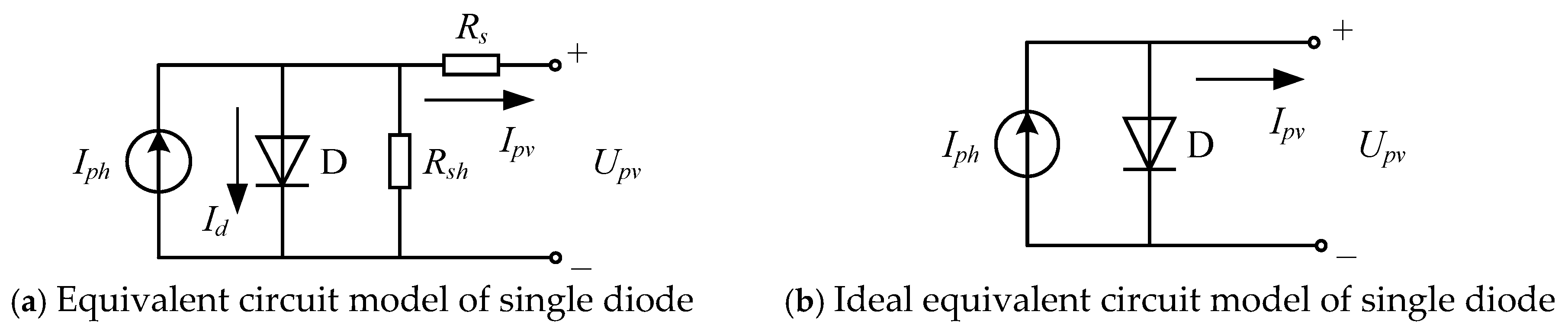
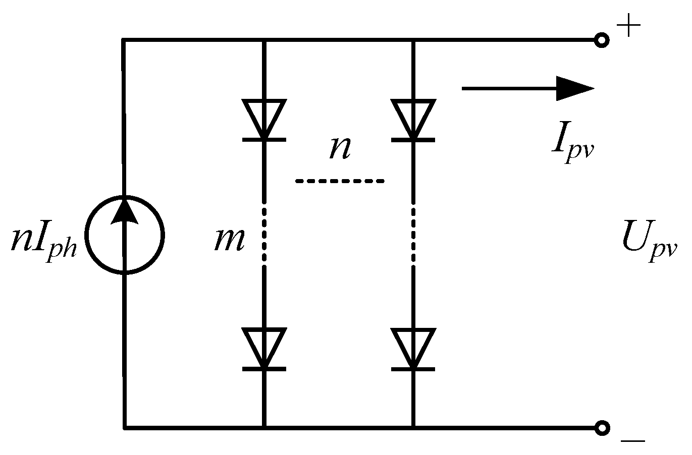
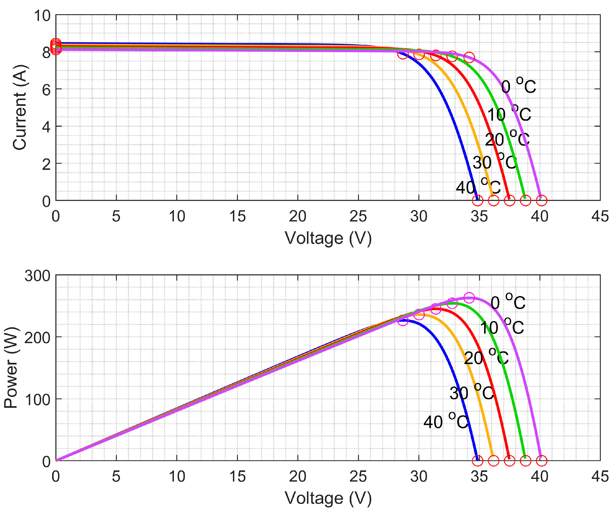
2.1. Characteristics of PV Panel

A PV array is a combination of many PV cells in series and parallel. The PV cell’s equivalent circuit model of a single diode is shown in Figure 1a. Here, I_ph represents the photocurrent which is proportional to the actual irradiance and ambient temperature; the diode describes the nonlinear relationship between the PV cell’s terminal voltage and current, with its current represented by I_d; R_sh is the equivalent bypass resistance; R_s is the equivalent series resistance; and the terminal voltage and current of the PV cell are symbolized with U_pv and I_pv, respectively. Since the magnitude of R_sh is very large and that of R_s very small, we can obtain the PV cell’s ideal equivalent circuit model depicted in Figure 1b by ignoring R_sh and R_s.

On the basis of the ideal equivalent circuit model and the PN junction’s characteristics of the diode, the mathematical model of the PV cell can be built as follows:

$$I_{pv}=I_{ph}-I_d=I_{ph}-I_0\left[\exp \left({\displaystyle \frac{q{U}_{pv}}{AkT}}-1\right)\right]$$

(1)

$$U_{pv}={\displaystyle \frac{AkT}{q}}\ln \left({\displaystyle \frac{I_{ph}}{I_0}}+1\right)$$

(2)

$$P_{pv}=U_{pv}{I}_{pv}$$

(3)

where I₀ is the diode’s reverse saturation current; A is the diode factor; q is the electron charge; k is the Boltzmann constant; T is the absolute temperature; and P_pv denotes the generated power of the PV cell.

Furthermore, based on the ideal model of the PV cell, we can construct the ideal equivalent circuit model (pictured in Figure 2) of the PV panel which comprises m PV cells in series and n strings in parallel.

Accordingly, we can derive the generated photocurrent by the following:

$$I_{pv}=n{I}_{ph}-n{I}_0\left[\exp \left({\displaystyle \frac{q{U}_{pv}}{AkTm}}-1\right)\right]$$

(4)

Given the specific illumination conditions, the power–voltage (P-U) and current–voltage (I-U) curves can be drawn demonstrating the relationship between the PV output power, terminal voltage, and output current. Figure 3 shows a typical family of P-U and I-U curves of a PV panel under consistent irradiance (1000 W/m²) and varying temperature (0–40 °C). We recognize that the P-U curves display a single-peak pattern under uniform illumination conditions. That is, there is only one MPP corresponding to a single voltage value (named as V_MPP) and a single current (named as I_MPP) because the maximum output power equals the product of V_MPP and I_MPP.

Obviously, the MPP’s position is not constant on the coordinate plane under the effect of the illumination condition. In other words, the MPP shifts in accordance with the actual irradiance and temperature. For instance, when the temperature changes, the values of the PV’s terminal voltage and output current at the MPP also change accordingly. Since the variations in V_MPP and I_MPP nonlinearly depend upon the environmental factors of irradiance and temperature, such a phenomenon naturally inspires us to fit this nonlinear relationship through machine learning.

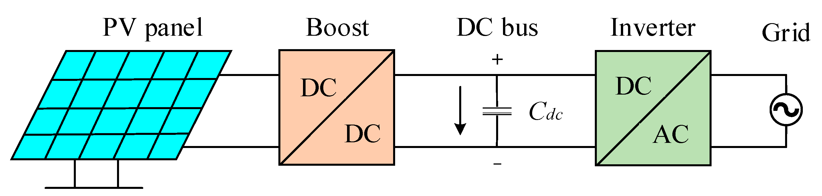
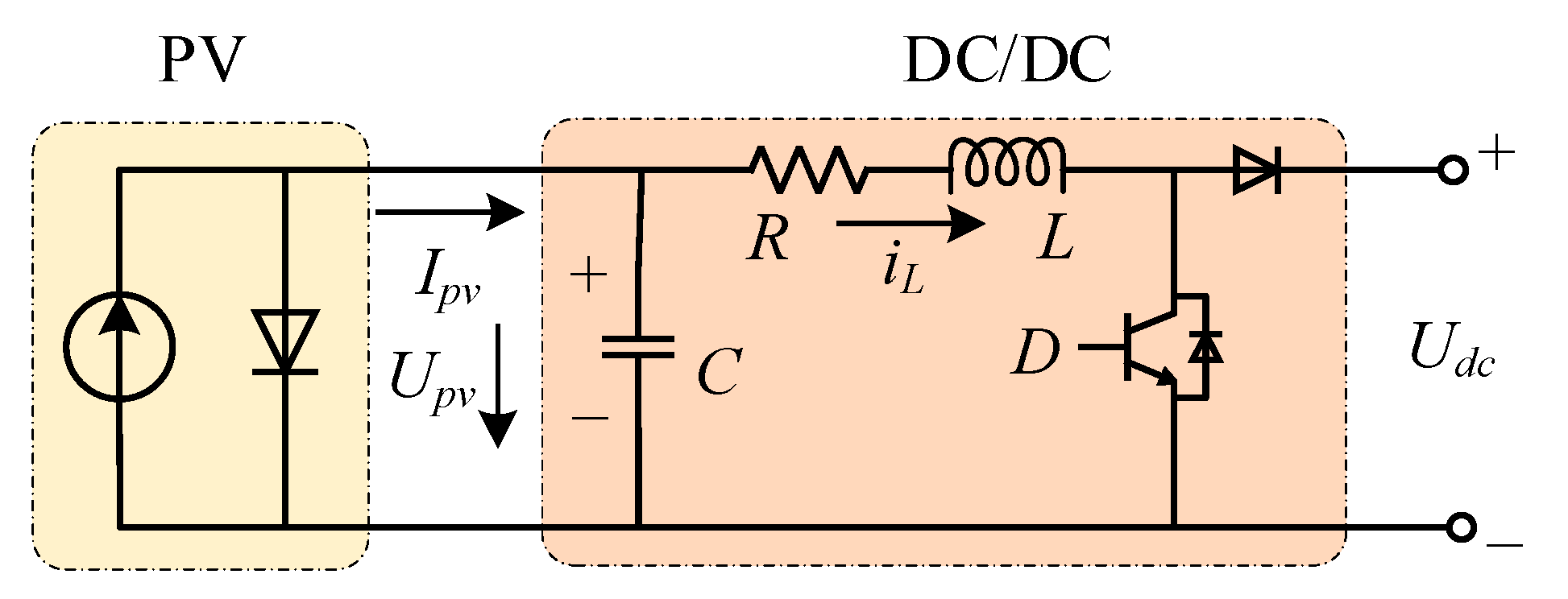
2.2. Structure of PV Power Generation System

In real applications, the two-stage grid-connected PV power generation system is an effective solution for achieving the high-efficiency utilization of solar energy. Its structure chart is depicted in Figure 4. The main tasks of the back-stage DC/AC inverter are to transfer the PV-generated power to the grid and to guarantee the DC bus voltage’s stability. Provided that the DC bus voltage is constant, then the front-stage DC/DC can achieve MPPT through adjusting its duty cycle to regulate the PV output current to its reference value at the MPP in real time, i.e., by letting I_pv approach I_MPP.

Consequently, we can draw the schematic diagram explaining the implementation of MPPT via the technique of current prediction and regulation in Figure 5. It is noticeable that the presented control scheme consists of two layers. The upper layer indeed plays the role of decision-making, i.e., generating the reference signal for the lower layer with the input information of irradiance and temperature; then, after receiving the reference value, the lower layer executes the current-tracking control. Only if each layer operates effectively and collaborates reliably with the other can the realization of MPPT be guaranteed. In this work, the function of I_MPP prediction in the upper layer is fulfilled through the SVR model whose hyperparameters are optimized by the SSA to attain high precision and a rapid convergence rate; in the lower layer, the LQ strategy is applied to realize PV’s output current regulation with satisfactory dynamic and steady-state performances.

2.3. Modeling of PV Generation System

As narrated in Section 2.2, in the scope of MPPT control, the PV system of interest consists of the PV panel and the DC/DC converter practically. The typical topology of a PV system is shown in Figure 6.

Provided that the DC bus voltage is constant, we can build the small-signal state-space model of the PV system as follows [35]:

$$\left\{\begin{array}{l}{\dot{x}}_1={\displaystyle \frac{1}{C{R}_{pv}}}{x}_1-{\displaystyle \frac{1}{C}}{x}_2\hfill \\ {\dot{x}}_2={\displaystyle \frac{1}{L}}{x}_1-{\displaystyle \frac{R}{L}}{x}_2+{\displaystyle \frac{U_{dc}}{L}}u\hfill \\ y=x_2\hfill \end{array}\right.$$

(5)

where x₁ is the small signal of the PV module output current U_pv; x₂ is the small signal of the inductance current i_L; u is the control input, that is, the PWM signal of the DC/DC; y is the system output; R_pv is the equivalent dynamic internal resistance of the PV panel; and U_dc is the DC bus voltage. It is apparent from Figure 6 and the first state equation in (5) that i_L equals I_pv when the system reaches a steady state.

In agreement with Equation (5), we can rewrite the PV system’s model in the following form:

$$\left\{\begin{array}{l}\dot{\mathit{x}}=A\mathit{x}+Bu\hfill \\ y=C\mathit{x}\hfill \end{array}\right.$$

(6)

where the matrices A, B, and C represent the system matrix, input matrix, and output matrix, respectively. And they are as follows:

$$A=\left[\begin{array}{cc}{\displaystyle \frac{1}{C{R}_{pv}}}& -{\displaystyle \frac{1}{C}}\\ {\displaystyle \frac{1}{L}}& -{\displaystyle \frac{R}{L}}\end{array}\right],B=\left[\begin{array}{c}0\\ {\displaystyle \frac{U_{dc}}{L}}\end{array}\right],C=\left[\begin{array}{cc}0& 1\end{array}\right]$$

When the parameters of the topology in Figure 6 are determined, the value of each element in matrices A, B, and C can be attained after simple calculation. Subsequently, we can develop the current regulator based on the PV system’s state-space model.

3. Constructing the Current Prediction Model

3.1. Support Vector Regression

Support vector regression (SVR) is the variant of the support vector machine applied in solving a regression problem, which is based on statistical learning theory with a loss function called the ε-insensitive loss function. SVR possesses a good generalization ability on the basis of the structural risk minimization principle and boasts small sample learning and a global optimization ability compared with an ANN [36,37].

Suppose we have a training dataset as follows:

$$S=\left\{({\mathit{x}}_1,y_1),\dots ,({\mathit{x}}_l,y_l)|{\mathit{x}}_{\mathrm{i}}\in R^n,y_j\in R\right\}$$

(7)

where x denotes the predictor variable and y represents the dependent variable.

Then, the goal of modeling the nonlinear relationship between x and y is to find a function f(x) satisfying the following equation:

$$|y_i-f({\mathit{x}}_i)|\le \epsilon ,\forall ({\mathit{x}}_i,y_i)\in S$$

(8)

And the nonlinear regression function f(x) is of the form as follows:

$$f\left(\mathit{x}\right)=(w\cdot \varphi (\mathit{x}\left)\right)+b$$

(9)

where w is the weight vector, b is the bias, and ϕ is the nonlinear function.

If the prediction error is less than ε, then it is taken as zero. Hence, the ε-insensitive loss function turns the nonlinear regression problem into an optimization problem as follows:

$$\left\{\begin{array}{l}\min {\displaystyle \frac{1}{2}}\Vert w{\Vert }^2\hfill \\ s.t.\left|y_i-f\left({\mathit{x}}_i\right)\right|\ll \epsilon ,i=1,2,\dots ,l\hfill \end{array}\right.$$

(10)

Through introducing slack variables ξ and ξ^* and regularization parameter C, Equation (10) turns into the following form:

$$\left\{\begin{array}{c}\min \left\{{\displaystyle \frac{1}{2}}\Vert w{\Vert }^2+C{\displaystyle \sum _{i=1}^L\left({\xi }_i+{\xi }_i^{*}\right)}\right\}\\ y_i-w\cdot \varphi \left({\mathit{x}}_i\right)-b\le {\xi }_i+\epsilon \\ s.t.w\cdot \varphi \left({\mathit{x}}_i\right)-y_i+b\le {\xi }_i^{*}+\epsilon \\ {\xi }_i,{\xi }_i^{*}\ge 0,i=1,2,\dots ,l\end{array}\right.$$

(11)

Furthermore, in order to solve the optimization problem simply, with the introduction of Lagrangian α and α^*, we can obtain the dual form of Equation (11) as follows:

$$\left\{\begin{array}{c}\max \left\{\begin{array}{l}-{\displaystyle \frac{1}{2}}{\displaystyle \sum _{i,j=1}^l({\alpha }_i-{\alpha }_i^{*}\left)\right({\alpha }_j-{\alpha }_j^{*})<\varphi \left({\mathit{x}}_i),\varphi \right({\mathit{x}}_j)}>\hfill \\ +{\displaystyle \sum _{i=1}^l{y}_i({\alpha }_i-{\alpha }_i^{*})}-\epsilon {\displaystyle \sum _{i=1}^l({\alpha }_i+{\alpha }_i^{*})}\hfill \end{array}\right\}\\ s.t.{\displaystyle \sum _{i=1}^l({\alpha }_i-{\alpha }_i^{*})=0,0\le {\alpha }_i,{\alpha }_i^{*}\le C,i=1,2,\dots ,l}\end{array}\right.$$

(12)

By replacing the dot product of the input vectors with the kernel function, we obtain the following SVR model.

$$f(\mathit{x})={\displaystyle \sum _{i=1}^l({\alpha }_i-{\alpha }_i^{*})K({\mathit{x}}_i,\mathit{x})+b}$$

(13)

where $K({\mathit{x}}_i,\mathit{x})$ represents the kernel function which can take the forms of being linear, Gaussian, polynomial, etc. For instance, the Gaussian kernel function’s expression is as follows:

$$K({\mathit{x}}_i,\mathit{x})=\exp \left(-g\Vert {\mathit{x}}_i-\mathit{x}{\Vert }^2\right)$$

(14)

where g is the parameter to be determined.

Last but not least, when applying SVR to construct the current prediction model for MPPT, some key points should be noted.

(1)

Data preprocessing

With the aim of improving the training effect of the SVR model, the original dataset must be preprocessed, for example, through dataset splitting and data normalization. In this study, the original data comprises three vectors, i.e., two input vectors of irradiance and temperature and one output vector of the current at the MPP. Let Irr and T symbolize the preprocessed input vectors and I_MPP the output vector. The objective of SVR modeling is to fit the input–output relationship by minimizing the error between the real value of I_MPP and its predicted value as follows:

$$\widehat{y}=f\left(\mathit{x}\right)$$

(15)

where $\mathit{x}=\left(Irr,T\right)$, and $\widehat{y}$ denotes the predicted value of the reference current at the MPP.

(2)

Hyperparameter optimization

The SVR model’s performance strongly relies on the hyperparameters’ selection. As can be recognized from Section 3.1, the SVR’s hyperparameters mainly include the regularization parameter C, the kernel function’s parameter g, and the error boundary ε. For the purpose of obtaining optimized hyperparameters through a more efficient approach compared to traditional methods like a grid search and cross validation, we decide to employ a heuristic algorithm with a better global search ability to accomplish this task.

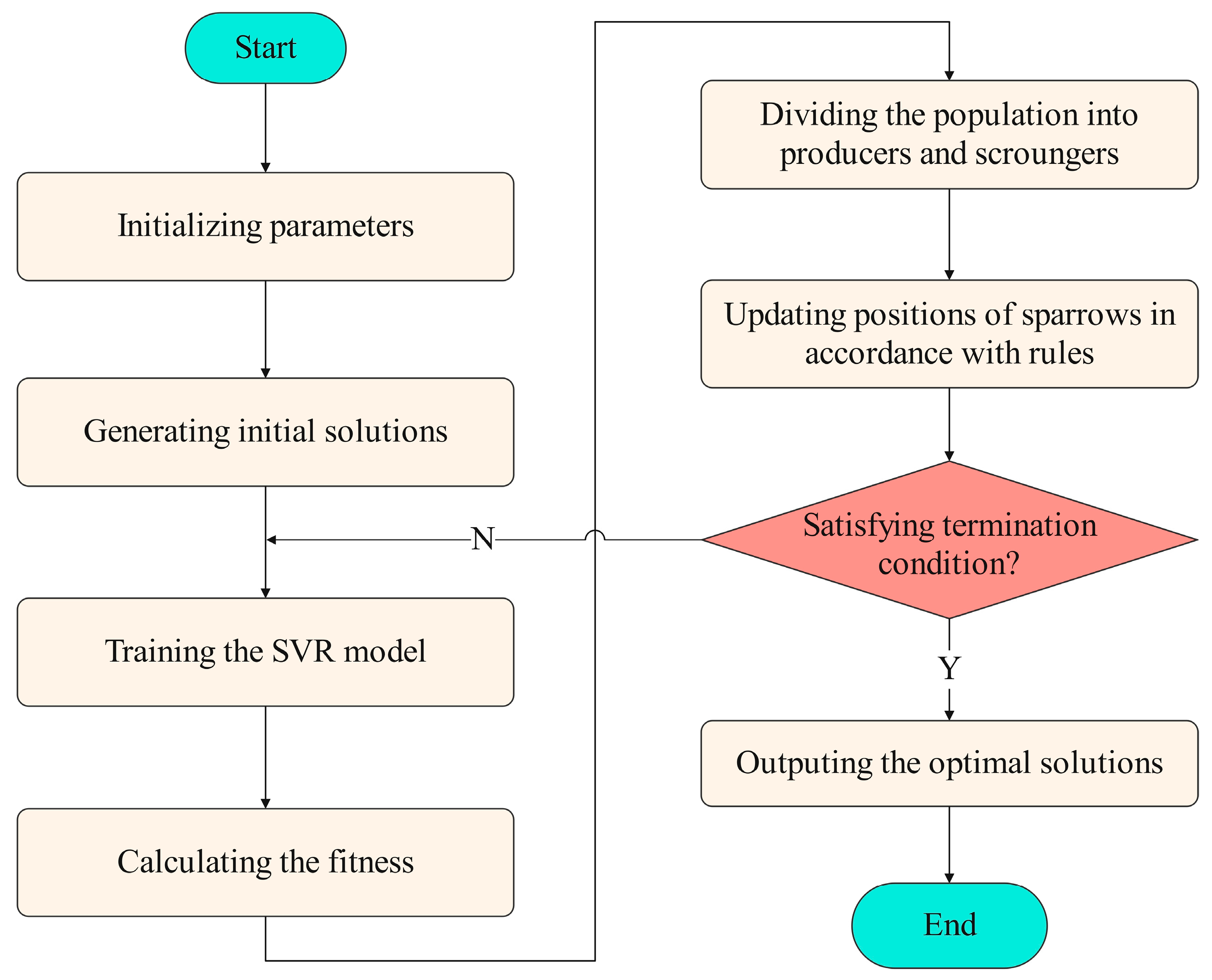
3.2. Sparrow Search Algorithm

The SSA is a novel swarm intelligence optimization approach proposed by Xue and Shen [38]. They have proved that the SSA surpasses PSO and GWO in terms of accuracy, convergence speed, stability, and robustness through a benchmark functions’ test. The SSA mimics the behavior of sparrows in nature. A group of sparrows is composed of two categories: the producers and the scroungers. The former group searches for the food source or provides directions to the food sources, while the latter group finds the food source. The role of each sparrow can switch between the producer and the scrounger. Additionally, several sparrows are responsible for sounding the alarm when discovering predators during food-searching [39].

To translate the sparrows’ behavior into an optimization algorithm, some necessary rules are summarized and listed as follows [40,41,42]:

(1)

The producers responsible for locating areas with abundant food have higher fitness than the scroungers. The fitness is determined by an optimized objective function.

(2)

If a predator is perceived and the corresponding alarm value exceeds the threshold, the producers will direct the scroungers to the safe place.

(3)

A scrounger can become a producer if its fitness is better. However, the total number of each group remains unchanged; i.e., a producer will turn into a scrounger accordingly.

(4)

Scroungers follow the producer with best fitness. During the food-searching process, hungry scroungers with low fitness tend to change their positions to improve their fitness.

(5)

The sparrows at the edge of the group will promptly fly to a safe area in case of danger, while the sparrows in the center of the group randomly move to the rest of the group.

In compliance with the above rules, the mathematical description of the SSA is as follows:

Assuming that the population size of sparrows is N and the dimension of the variables to be optimized is D, then the position matrix of all sparrows can be defined as follows:

$$X=\left[\begin{array}{cccc}{X}_{1,1}& X_{1,2}& \dots & X_{1,D}\\ X_{2,1}& X_{2,2}& \dots & X_{2,D}\\ ⋮& ⋮& ⋮& ⋮\\ X_{N,1}& X_{N,2}& \dots & X_{N,D}\end{array}\right]$$

(16)

Next, the fitness values of all sparrows can be expressed as a vector:

$$F_X=\left[\begin{array}{c}f\left(\left[X_{1,1}{X}_{1,2}\dots X_{1,D}\right]\right)\\ f\left(\left[X_{2,1}{X}_{2,2}\dots X_{2,D}\right]\right)\\ ⋮\\ f\left(\left[X_{N,1}{X}_{N,2}\dots X_{N,D}\right]\right)\end{array}\right]$$

(17)

In agreement with rule (1) and rule (2), the update law of the producer at each iteration is as follows:

$$X_{i,j}^{t+1}=\left\{\begin{array}{ll}{X}_{i,j}^t\cdot \exp \left({\displaystyle \frac{-i}{\alpha ·{iter}_{\max }}}\right)\hfill & R<ST\hfill \\ X_{i,j}^t+Q\cdot L\hfill & R\ge ST\hfill \end{array}\right.$$

(18)

where t denotes the current iteration, the maximum number of iterations is iter_max, α is a random number belonging to (0, 1], Q is a random number obeying the normal distribution, L is a vector with the length of D in which all elements equal 1, R represent the warning value which belongs to [0, 1], and ST, whose value falls in [0.5, 1], symbolizes the safety threshold. When R < ST, there are no predators around, and the producers can search for food in a larger range, but when R ≥ ST, the predators are detected, and thus all the sparrows fly to safe places rapidly.

With respect to the scroungers, in line with rule (3) and rule (4), their positions update according to the following law:

$$X_{i,j}^{t+1}=\left\{\begin{array}{ll}Q\cdot \exp \left({\displaystyle \frac{X_{worst}^t-X_{i,j}^t}{i^2}}\right)\hfill & i>\frac{n}{2}\hfill \\ X_P^{t+1}+\left|X_{i,j}^t-X_P^{t+1}\right|\cdot A^{+}\cdot L\hfill & i\le \frac{n}{2}\hfill \end{array}\right.$$

(19)

where X_worst signifies the current global worst position, and X_P signifies the current best position occupied by the producer. A is a vector with the length of D, in which each element is assigned a value of −1 or 1 randomly, and A⁺ = A^T(AA^T)⁻¹. When i > n/2, the ith scrounger is suffering from hunger and has to fly to other places to seek food. When i ≤ n/2, the ith scrounger will fly close to the best sparrow to find food.

The response strategy to danger is based on rule (5). The position-updating formula is expressed as follows:

$$X_{i,j}^{t+1}=\left\{\begin{array}{ll}{X}_{best}^t+\beta \cdot \left|X_{i,j}^t-X_{best}^t\right|\hfill & f_i\ne f_g\hfill \\ X_{i,j}^t+K\cdot \left({\displaystyle \frac{\left|X_{i,j}^t-X_{worst}^t\right|}{\left({\displaystyle f_i-f_w}\right)+ϵ}}\right)\hfill & f_i=f_g\hfill \end{array}\right.$$

(20)

where X_best is the current global best location; β is the step size, which is a random number subject to standard normal distribution; K is a random number belonging to [−1, 1], which decides the sparrow’s flying direction; f_i represents the fitness value of the ith sparrow; f_g and f_w are the best and worst fitness values of the current population, respectively; and $ϵ$ is a minimal positive real number lest the denominator equals zero.

By fusing the procedures of nonlinear modeling with SVR and its hyperparameters’ optimization with the SSA, we can draw the flowchart of SSA-SVR in Figure 7.

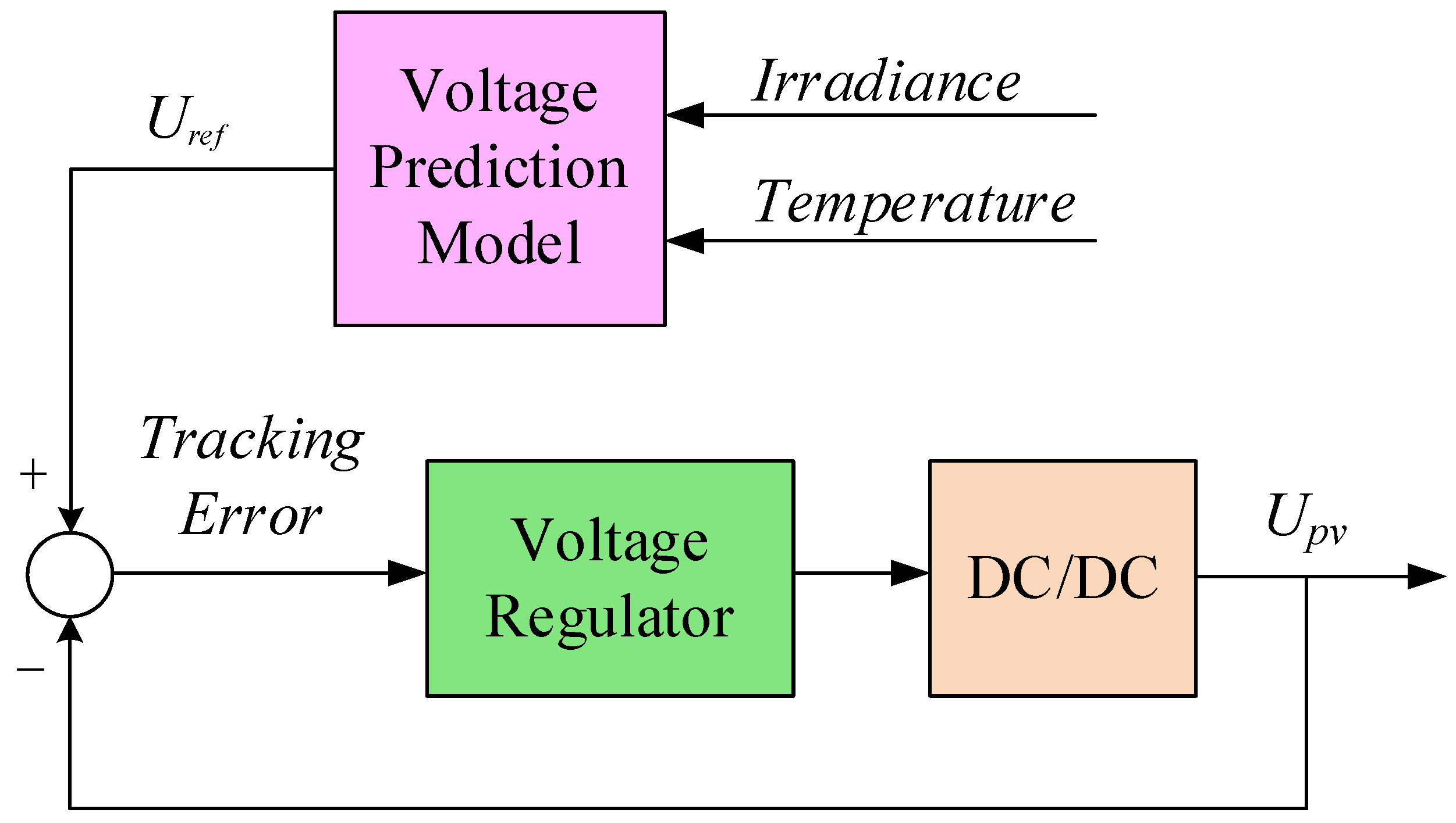
4. Robust Current-Tracking Controller Design

4.1. Problem Formulation

As analyzed in Section 2.2, the lower layer of the MPPT control actually regulates I_pv to its reference value I_MPP, and we can design the controller on the basis of the PV system’s state-space model. If there are no uncertainties like a model’s parameters’ perturbation, the variation in the reference input, and unknown disturbances, the controller design is a classic stabilization problem which can be solved by means of the pole placement method. However, there are some issues that should be addressed for this controller design strategy: (i) The position of poles decides the system’s dynamic response. Nevertheless, the determination of the poles’ anticipated position is not easy and generally depends on the designer’s experience. (ii) To improve the system’s comprehensive performance, we need to trade off the stability and other indexes, for instance, the overshoot, settling time, etc. (iii) The uncertainties exist objectively, so the controller must function properly under the uncertainties as well; i.e., the robustness is a necessary requirement for MPPT.

Concerning issues (i) and (ii), we propose designing the controller based on the linear quadratic optimal control, which can improve the system’s behavior by optimizing the performance index. The details on this trick are explained in Section 4.2. As for issue (iii), we turn the stabilization problem into a regulation problem by introducing a new state variable. The analysis procedure is as follows:

The regulation of the PV panel’s output current I_pv means moving it to its reference value I_MPP with zero steady-state errors; i.e., the tracking error approaches zero.

$$\underset{t\to \infty }{\lim }e\left(t\right)=\underset{t\to \infty }{\lim }\left[I_{pv}\left(t\right)-I_{MPP}\left(t\right)\right]=0$$

(21)

where e denotes the tracking error, and t is the time variable.

Since the effect of uncertainties will influence the tracking error, we therefore define a new state variable ξ as follows:

$$\dot{\xi }=e$$

(22)

It is apparent that when ξ → 0, the tracking error becomes close to zero too. In accordance with the built model in Equation (6), we can obtain the new variable’s state equation as follows:

$$\dot{\xi }=y-y_{ref}=C\mathit{x}-y_{ref}$$

(23)

where y_ref represents I_MPP.

By combining Equations (6) and (23), we obtain a new state-space model as follows:

$$\left[\begin{array}{c}\dot{\mathit{x}}\\ \dot{\xi }\end{array}\right]=\left[\begin{array}{cc}A& 0\\ C& 0\end{array}\right]\left[\begin{array}{c}\mathit{x}\\ \xi \end{array}\right]+\left[\begin{array}{c}B\\ 0\end{array}\right]u+\left[\begin{array}{c}0\\ -1\end{array}\right]y_{ref}$$

(24)

Finally, let $\mathit{z}={\left[\mathit{x},\xi \right]}^T$, $\tilde{A}=\left[\begin{array}{cc}A& 0\\ C& 0\end{array}\right]$, $\tilde{B}=\left[\begin{array}{c}B\\ 0\end{array}\right]$, $\tilde{C}=\left[\begin{array}{cc}C& 0\end{array}\right]$, $W=\left[\begin{array}{c}0\\ -1\end{array}\right]$; then, we rewrite the PV system’s model as follows:

$$\left\{\begin{array}{l}\dot{\mathit{z}}=\tilde{A}\mathit{z}+\tilde{B}u+W{y}_{ref}\hfill \\ y=\tilde{C}\mathit{z}\hfill \end{array}\right.$$

(25)

With this model, we adopt the following technique to design its controller.

4.2. Linear Quadratic Optimal Control

The linear quadratic (LQ) optimal control seeks to find a permissible control input to minimize the given energy-type performance index function as follows [30,43,44]:

$$J\left(u\left(\cdot \right)\right)={\displaystyle {\int }_0^{\infty }\left({\mathit{z}}^{T}Q\mathit{z}+u^{T}Ru\right)dt}$$

(26)

where z represents the state vector, u is the control input, and Q and R are the weighing matrices which are usually set as the symmetric positive definite matrix.

According to Equation (26), the LQ strategy is physically an optimal control strategy designed to stabilize a linear dynamic system while balancing two competing objectives, i.e., minimizing deviations in the system’s states from a desired equilibrium and the consumed energy with the application of the control input.

The permissible control is of the state feedback form as follows:

$$u^{*}\left(t\right)=-K^{*}{\mathit{x}}^{*}\left(t\right)$$

(27)

where u^* represents the optimal control, K^* is the optimal state feedback matrix, and x^* symbolizes the optimal trajectory of the state variables.

The optimal state feedback matrix is solved by the following:

$$K^{*}=R^{-1}{B}^{T}P$$

(28)

where matrix P is the unique symmetric positive definite solution of the following matrix Riccati algebraic equation.

$$P\tilde{A}+{\tilde{A}}^{T}P+Q-P\tilde{B}{R}^{-1}{\tilde{B}}^{T}P=0$$

(29)

Finally, yet importantly, it should be pointed out that before applying the LQ strategy to design the controller, the system must be controllable, which is readily verified using the rank criterion as follows:

$$Rank\left[\tilde{B},\tilde{A}\tilde{B},\dots ,{\tilde{A}}^{n-1}\tilde{B}\right]=n$$

(30)

where n is the system model’s order.

5. Results and Discussion

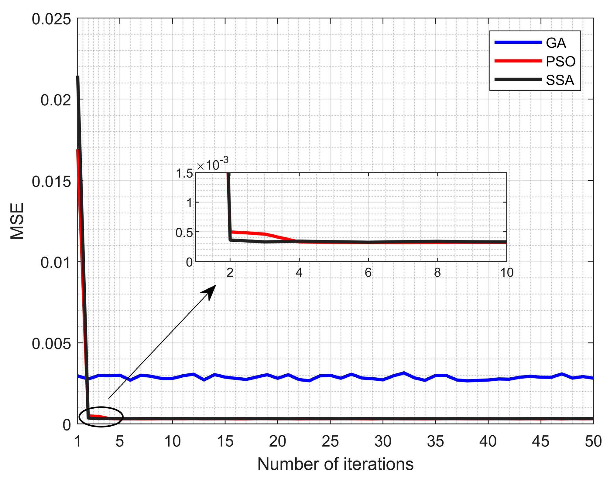
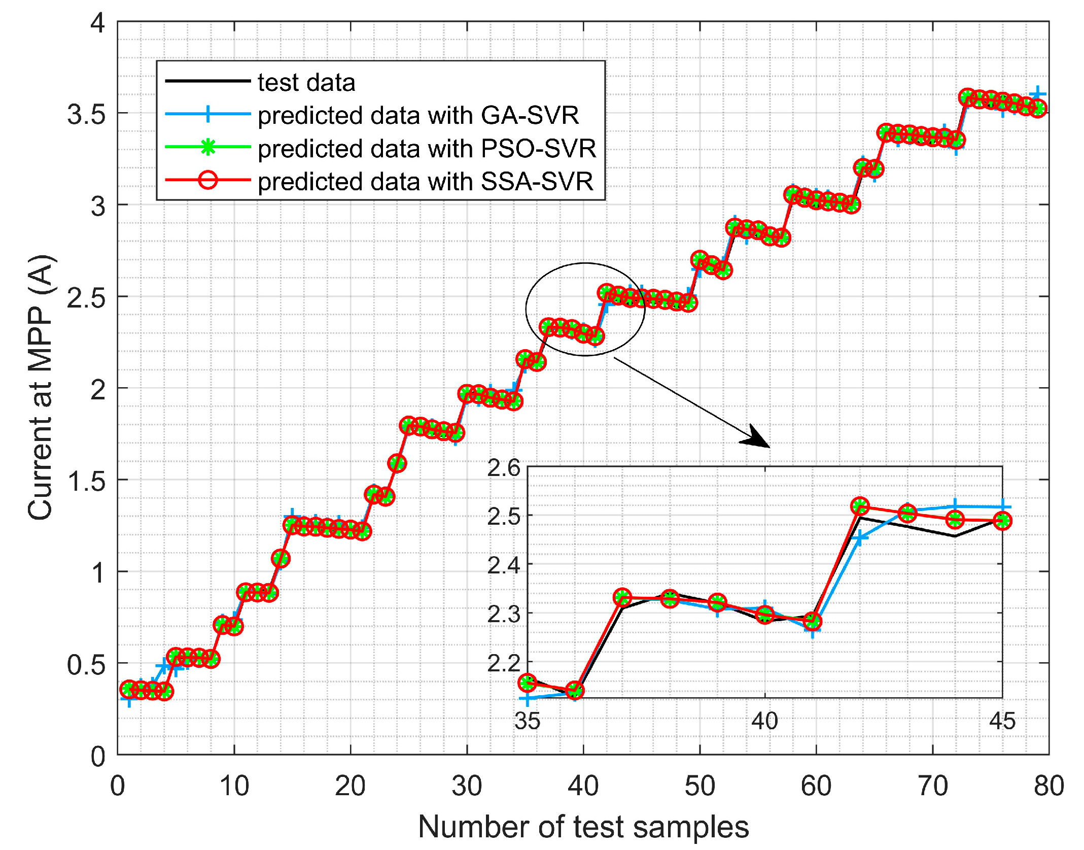
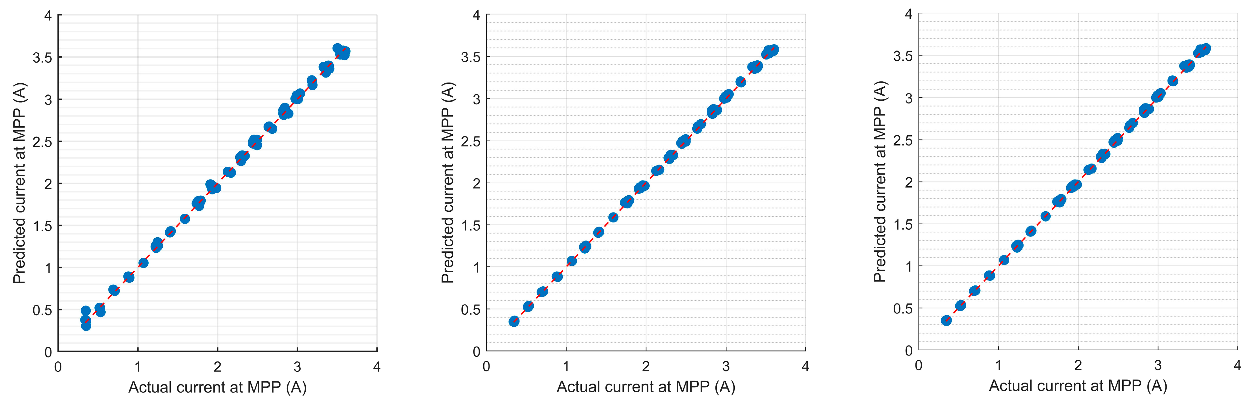
5.1. Predicting the Reference Current at the MPP Based on SSA-SVR

To verify the effectiveness and accuracy of predicting the reference current at the MPP through the presented SSA-SVR approach, we first train the SVR model with the dataset provided in [45]. The datasheet contains 27 × 399 data points corresponding to some variables such as temperature, irradiance, maximum power voltage, maximum power current, and many others (the number of variables is 27 and the length of each variable data is 399). Since we use the data for training the I_MPP prediction model, we then take the irradiance and temperature values from the original dataset as the input vectors of the SVR, and the maximum power current as the output vector. The dataset is divided into the training set (80% of the total data) and the test set (20% of the total data), which are normalized with a standard score before training and testing. As previously mentioned in Section 1, the GA and PSO are two typical heuristic algorithms successfully used for hyperparameter optimization. Therefore, we compare the performance between the SSA and optimizing the SVR’s hyperparameters C, g, and ε. The population size and the number of iterations for all three metaheuristic algorithms are uniformly set to 20 and 50, respectively. Additional parameter settings are listed in

Table 2. Parameter settings of selected metaheuristic algorithms.

Algorithm	Parameters
GA	crossover rate is 0.8; mutation rate is 0.01
PSO	inertia weight is 0.5; learning factors are 1.5
SSA	ST = 0.8; the proportion of producers is 70%

.

The optimal hyperparameters of SVR obtained by the GA, PSO, and the SSA are listed in

Table 3. Optimized hyperparameters of SVR with different metaheuristic algorithms.

Algorithm	C	g	ε
GA	343.9078	5.8824	0.0185
PSO	717.5694	0.01	0.01
SSA	1000	0.01	0.01

. The convergence performances are depicted in Figure 8. It is obvious that both PSO and the SSA outperform the GA in terms of prediction accuracy. The GA depends on fixed genetic operations, which lead to lower global search efficiency and a higher likelihood of premature convergence. The minimum errors achieved by PSO and the SSA are very close; however, the SSA ensures stronger robustness and a faster convergence rate. After just two iterations, the SSA converges near the optimal solution, and each subsequent iteration yields solutions remaining in close proximity to the optimal solution. Compared with the SSA, PSO searched the optimal solution at the fifth iteration, indicating a slower convergence rate. As PSO’s updating mechanism depends on both individual and global historical optima, its convergence is frequently hindered by parameter dependency.

To quantitatively compare the performance of these algorithms, the evaluation metrics are listed in

Table 4. Comparison of performance metrics.

Algorithm	MAE	MSE	RMSE	R2
GA	0.0262	0.0011	0.0334	0.9988
PSO	0.0116	0.00024	0.0151	0.9997
SSA	0.0102	0.00019	0.0139	0.9998

, including the mean absolute error (MAE), mean squared error (MSE), root mean squared error (RMSE), and coefficient of determination (R²). We can discern that the SSA exhibits optimal performance across all metrics. Clearly, the results demonstrate that the SSA is an excellent choice for the offline optimization of SVR’s hyperparameters.

Based on the three optimized SVR models, we further examine their prediction accuracy with test data. The results are shown in Figure 9. It is apparent that the SSA-SVR model can achieve the highest precision. Additionally, the scatter plots of the predicted values versus those of the actual values for each model are pictured in Figure 10. We recognize that all the points of the SSA-SVR and PSO-SVR models are closely clustered around the diagonal line, which also proves their excellent behavior. Since the SSA-SVR model excels in many aspects including the convergence rate, robustness, and precision, we decide to choose it as the preferred tool for predicting the reference current at MPP based on the measured irradiance and temperature.

Figure 11 shows the results of the case under real operational conditions in a day. Figure 11a depicts the trends of the measured irradiance and temperature from 8:00 to 17:00. The sample interval is 5 min; hence, there are 109 data points totally. The variation range of the irradiance is from 121.62 w/m² to 1053 w/m² and that of the temperature is from 27.76 °C to 54.18 °C. Figure 11b displays the predicted reference current at the MPP. It is evident that the trend of the output current from a PV panel is positively correlated with the irradiance, whereas the temperature exhibits a relatively weak influence on it. In conclusion, the higher the irradiance is, the greater I_MPP.

5.2. Performance Analysis of Current Regulation

On the basis of the controlled system’s state-space model and the current regulation strategy presented in Section 4.2, we can develop the regulator using the circuit parameters of the boost DC/DC converter outlined in

Table 5. Circuit parameters of the boost DC/DC.

Parameters	Description	Value	Unit
R	Input resistance of DC/DC	0.0005	Ω
L	Input inductance of DC/DC	0.002	H
C	Input capacitance of DC/DC	0.00047	F
Udc	DC bus voltage	100	V
Uoc	Open-circuit voltage of PV panel	20.6697	V
Isc	Short-circuit current of PV panel	3.8756	A
P	Maximum output power of PV panel	60	W
Rpv	Equivalent resistance of PV panel	5.3333	Ω

. It should be pointed out that two PV panels connected in parallel are configured in the simulation model.

The calculated matrices $\tilde{A}$ and $\tilde{B}$ of the state-space model (25) are as follows:

$$\tilde{A}=\left[\begin{array}{ccc}398.9387& -2127.7& 0\\ 500& -0.25& 0\\ 0& 1& 0\end{array}\right],\tilde{B}=\left[\begin{array}{c}0\\ 50000\\ 0\end{array}\right]$$

With the rank criterion given in (30), we verified that the pair $\left\{\tilde{A},\tilde{B}\right\}$ is completely controllable. Next, to derive the optimal state feedback matrix K^*, the weight matrices R and Q must be chosen in advance. Through integrating Bryson’s Rule with the trial-and-error method, we ultimately selected the weight matrices as R = 10 and Q = diag(0.1, 0.1, 1 × 10⁴). Then, based on the determined R and Q, we can obtain the following optimal state feedback matrix.

$$K^{*}=\left[\begin{array}{ccc}0.1386& -0.1433& 31.6228\end{array}\right]$$

(1)

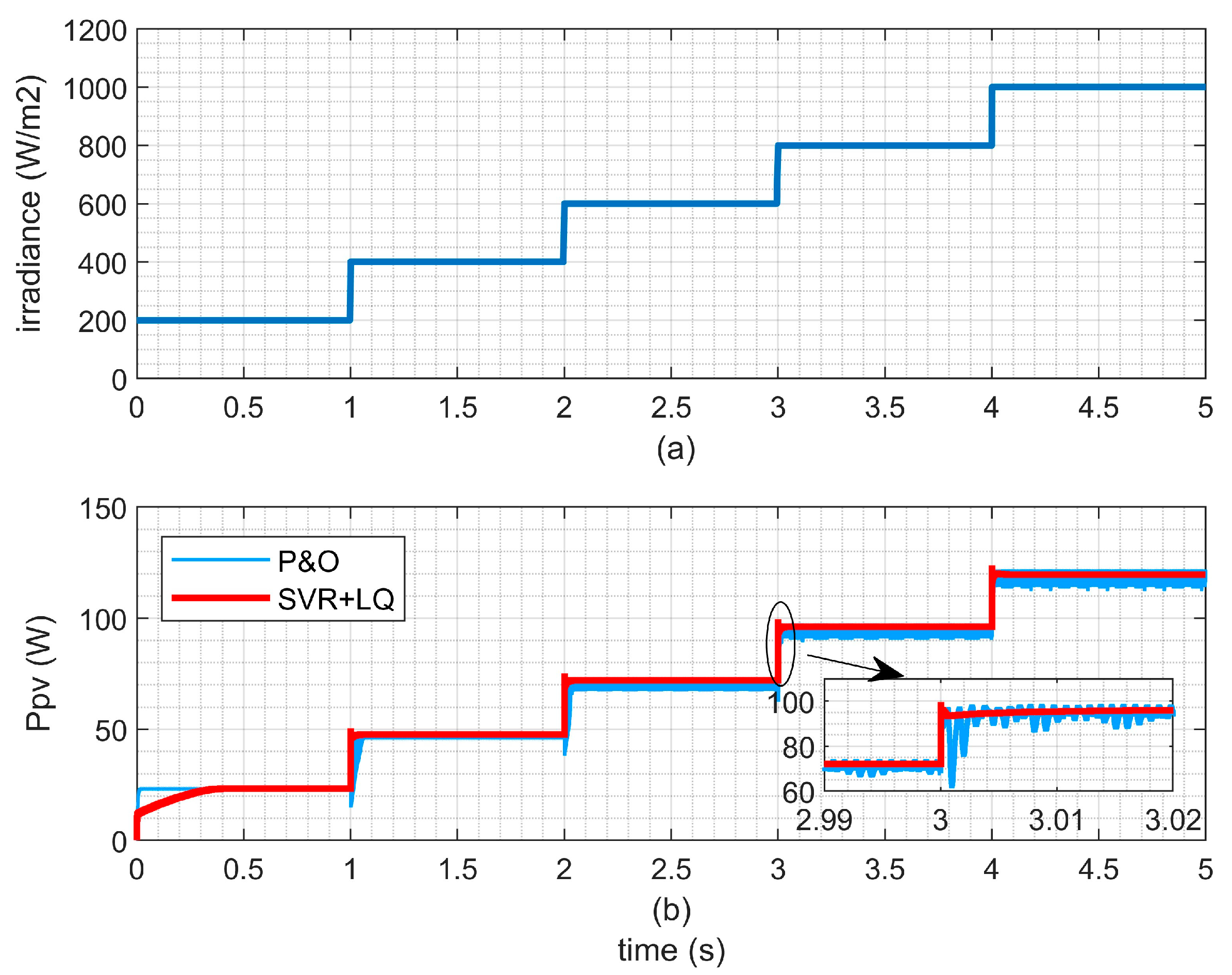
Performance Comparison between the Current Regulator and P&O

To evaluate the MPPT performance of the proposed current regulator, we conducted the simulation under varying irradiance conditions. The irradiance ranged from 200 W/m² to 1000 W/m², and the temperature was maintained at 25 °C. The responses of the LQ-based current regulator and P&O are plotted in Figure 12. Obviously, both methods are capable of achieving MPPT. However, according to the enlarged details, the current regulation approach demonstrates superior stability and accuracy compared to the P&O method.

(2)

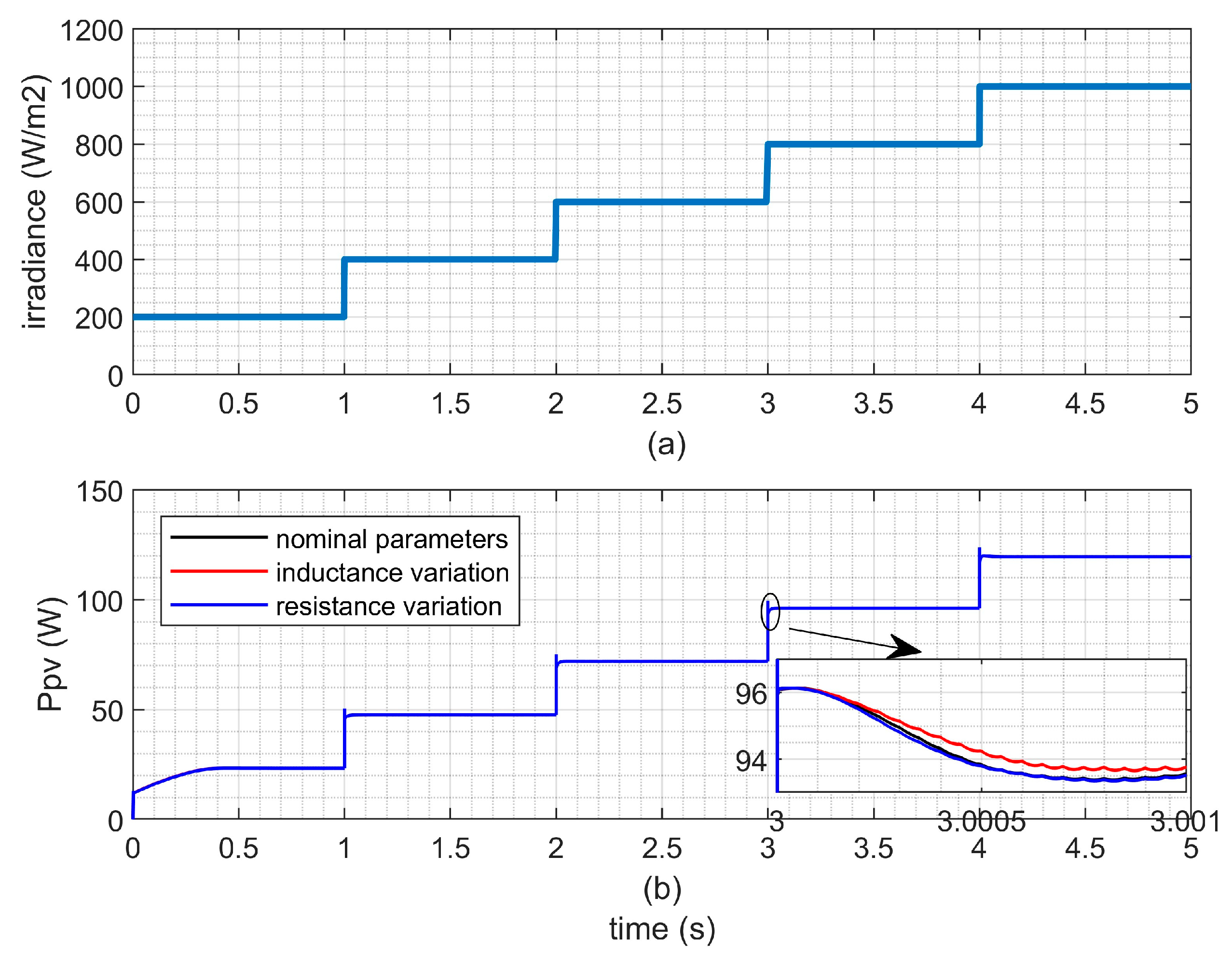
Robustness Analysis of the Current Regulator

The presented current regulator is essentially a kind of model-based technique. The designed optimal state feedback matrix K^* is calculated with the nominal parameters of the controlled system. Therefore, it is essential to further examine its robustness under parameter perturbations. In this simulation, the settings of irradiance and temperature are consistent with those in Figure 13, R and L of the DC/DC circuit (in Figure 6) are selected to be tested, and the two cases are considered. They are as follows: the perturbed value of R is twice its nominal value and that of L is half its nominal value as listed in Table 4. The results are depicted in Figure 13. We observe that responses under the three parameter configurations are very close, which proves that the proposed current regulator possesses strong robustness.

(3)

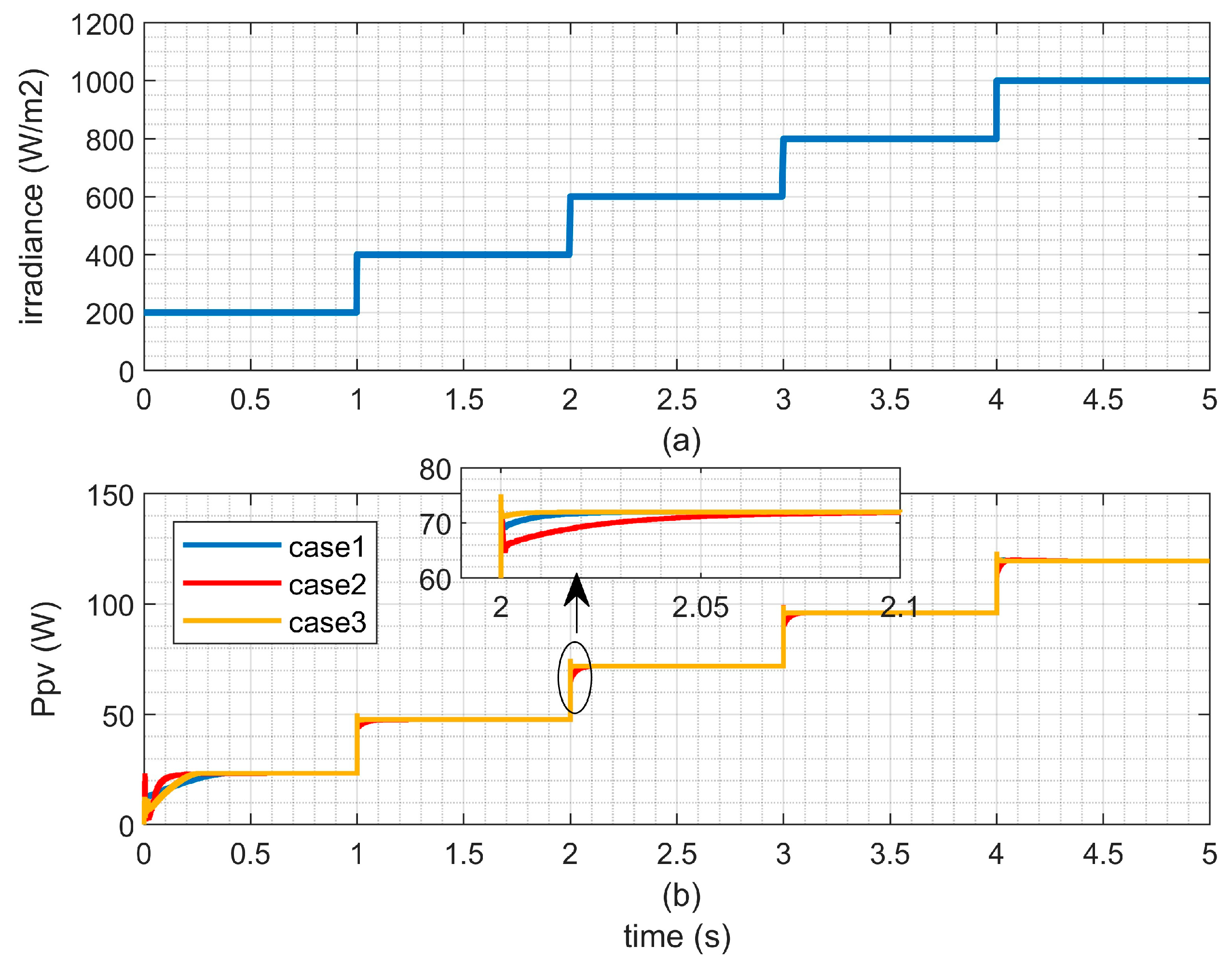
Performance Analysis of LQ Strategy with Different Weighing Matrices

The determination of the weighting matrices Q and R will influence the control effects of the LQ strategy. Generally, increasing the elements of matrix Q facilitates faster convergence of the state variables, but this may lead to excessive control inputs or actuator saturation. Meanwhile, raising the elements of matrix R tends to reduce the energy consumption of the control inputs, but this may result in a slower dynamic response. To validate the effects influenced by the weighting matrices, we conducted a performance comparison among the three different settings of Q and R, i.e., Case 1: R = 10 and Q = diag(0.1, 0.1, 1 × 10⁴); Case 2: R = 100 and Q = diag(0.1, 0.1, 1 × 10³); and Case 3: R = 1 and Q = diag(0.1, 0.1, 1 × 10⁵). The results are shown in Figure 14. It is apparent that Case 1 presents the most satisfactory comprehensive performance. Consequently, we select this configuration as the final choice for matrices Q and R.

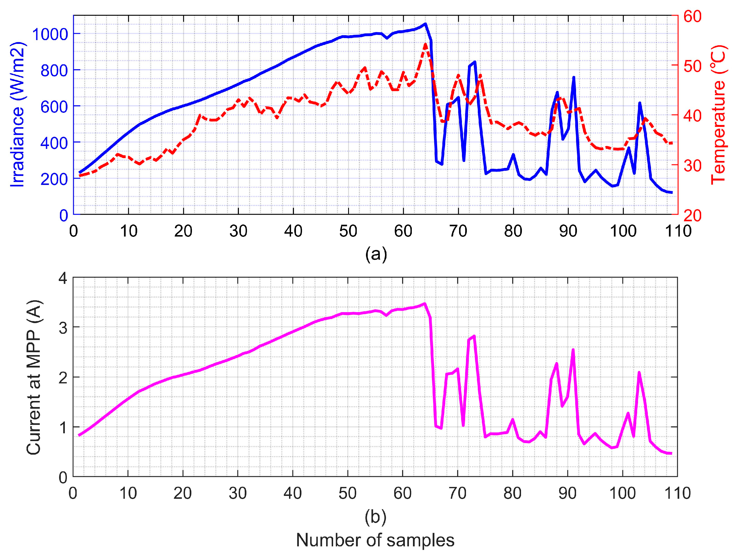
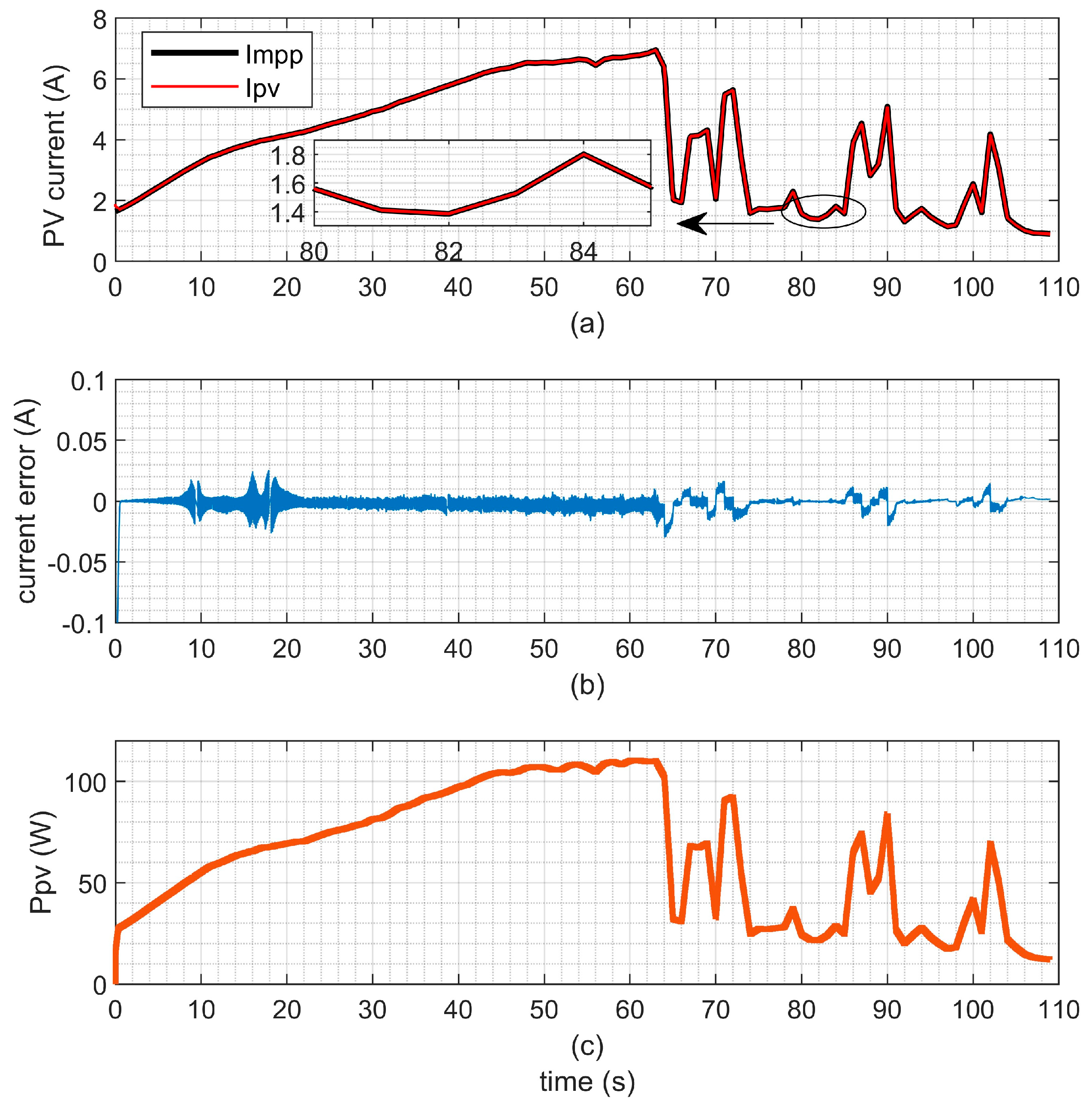
5.3. Effect Verification of MPPT with the Measured Irradiance and Temperature of a Day

For validating the effects of the proposed MPPT algorithm under real environmental conditions, the predicted current at the MPP shown in Figure 11 is set as the reference signal for the current regulator. To improve simulation efficiency, the timescale of the reference current samples is scaled into a 1 s interval. The current-tracking performance is illustrated in Figure 15a. It is apparent that the PV output current maintains tight proximity to the reference current. Figure 15b shows the tracking errors. We can see that the error approaches zero throughout the whole process. The maximum absolute error is 0.03 A and the mean absolute error is 0.0034 A, which demonstrate high tracking accuracy. The PV output power is shown in Figure 15c. The results confirm that the proposed SSA-SVR-LQ strategy can achieve the function of MPPT with satisfactory performance.

6. Conclusions

This study focuses on the MPPT control problem of the PV system. A complete control scheme, including predictions of the reference current at the MPP and PV output current regulation, is proposed. To achieve high-precision predictions, the SVR method is suggested. Besides that, the SSA is utilized to optimize the hyperparameters of the SVR to ensure better performance. For the purpose of acquiring satisfactory comprehensive performance of the controlled system, the LQ optimal control strategy is introduced to design the optimal regulator. The effectiveness of the presented control scheme is validated through simulations with multiple cases and the following conclusions are drawn:

(1)

SSA-SVR is an effective tool to model the nonlinear relationship among irradiation, temperature, and the PV output currents at the MPP. In comparison with other modeling methods in the same test conditions, SSA-SVR can give better prediction results.

(2)

The adopted LQ optimal control can both ensure the controlled system’s stability, steady-state performance, and strong robustness under uncertainties of parameter perturbation and disturbances and also achieve a satisfactory dynamic response during the regulating process.

While the excellent performance of the proposed SSA-SVR-LQR scheme is demonstrated with some cases and real measured data, the results are limited to simulations, and the dataset used to train the SVR model does not cover the conditions of partial shading. Hence, based on the work of this article, the authors will in the future further strive to apply the scheme in the real system and address the MPPT problem under more complicated scenarios.

References

1. Vodapally, S.N.; Ali, M.H. A Comprehensive Review of Solar Photovoltaic (PV) Technologies, Architecture, and Its Applications to Improved Efficiency. Energies 2023, 16, 319. [Google Scholar] [CrossRef]
2. Shakeel, S.R.; Yousaf, H.; Irfan, M.; Rajala, A. Solar PV adoption at household level: Insights based on a systematic literature review. Energy Strateg. Rev. 2023, 50, 101178. [Google Scholar] [CrossRef]
3. Huang, C.; Yan, Y.; Madonski, R.; Zhang, Q.; Deng, H. Improving operation strategies for solar-based distributed energy systems: Matching system design with operation. Energy 2023, 276, 127610. [Google Scholar] [CrossRef]
4. Zidane, T.E.K.; Aziz, A.S.; Zahraoui, Y.; Kotb, H.; Aboras, K.M.; Kitmo; Jember, Y.B. Grid-connected Solar PV power plants optimization: A review. IEEE Access 2023, 11, 79588–79608. [Google Scholar] [CrossRef]
5. Katche, M.L.; Makokha, A.B.; Zachary, S.O.; Adaramola, M.S. A Comprehensive Review of Maximum Power Point Tracking (MPPT) Techniques Used in Solar PV Systems. Energies 2023, 16, 2206. [Google Scholar] [CrossRef]
6. Sharma, S.; Jately, V.; Kuchhal, P.; Kala, P.; Azzopardi, B. A Comprehensive Review of Flexible Power-Point-Tracking Algorithms for Grid-Connected Photovoltaic Systems. Energies 2023, 16, 5679. [Google Scholar] [CrossRef]
7. Ramírez Torres, J.A.; Lastres Danguillecourt, O.; González Domínguez, R.A.; Ibáñez Duharte, G.R.; Verea Valladares, L.E.; Pantoja Enríquez, J.; Enríquez Santiago, J.A.; López López, A.; Verde Añorve, A. Development and Implementation of the MPPT Based on Incremental Conductance for Voltage and Frequency Control in Single-Stage DC-AC Converters. Energies 2025, 18, 184. [Google Scholar] [CrossRef]
8. Khan, M.A.; Usama, M.; Kim, J. Deep Symbolic Regression-Based MPPT Control for a Standalone DC Microgrid System. Energies 2024, 17, 6377. [Google Scholar] [CrossRef]
9. Mahdi, A.S.; Mahamad, A.K.; Saon, S.; Tuwoso, T.; Elmunsyah, H.; Mudjanarko, S.W. Maximum power point tracking using perturb and observe, fuzzy logic and ANFIS. Sn Appl. Sci. 2020, 2, 89. [Google Scholar] [CrossRef]
10. Podder, A.K.; Roy, N.K.; Pota, H.R. MPPT methods for solar PV systems: A critical review based on tracking nature. IET Renew. Power Gen. 2019, 13, 1615–1632. [Google Scholar] [CrossRef]
11. Zhang, Y.; Wang, H.; Zhu, X. Hybrid maximum power point tracking control method for photovoltaic power generation systems. J. Power Electron. 2023, 23, 1542–1550. [Google Scholar] [CrossRef]
12. Manna, S.; Akella, A.K.; Singh, D.K. Novel Lyapunov-based rapid and ripple-free MPPT using a robust model reference adaptive controller for solar PV system. Prot. Contr Mod. Pow. 2023, 8, 13–25. [Google Scholar] [CrossRef]
13. Feroz Mirza, A.; Mansoor, M.; Ling, Q.; Khan, M.I.; Aldossary, O.M. Advanced Variable Step Size Incremental Conductance MPPT for a Standalone PV System Utilizing a GA-Tuned PID Controller. Energies 2020, 13, 4153. [Google Scholar] [CrossRef]
14. Harrag, A.; Messalti, S. Variable step size modified P&O MPPT algorithm using GA-based hybrid offline/online PID controller. Renew. Sustain. Energy Rev. 2015, 49, 1247–1260. [Google Scholar]
15. Elobaid, L.M.; Abdelsalam, A.K.; Zakzouk, E.E. Artificial neural network-based photovoltaic maximum power point tracking techniques: A survey. IET Renew. Power Gen. 2015, 9, 1043–1063. [Google Scholar] [CrossRef]
16. Venkata Mahesh, P.; Meyyappan, S.; Alla, R. Support Vector Regression Machine Learning based Maximum Power Point Tracking for Solar Photovoltaic systems. Int. J. Electr. Comput. 2023, 14, 100–108. [Google Scholar] [CrossRef]
17. Roy, B.; Adhikari, S.; Datta, S.; Devi, K.J.; Devi, A.D.; Ustun, T.S. Harnessing Deep Learning for Enhanced MPPT in Solar PV Systems: An LSTM Approach Using Real-World Data. Electricity 2024, 5, 843–860. [Google Scholar] [CrossRef]
18. Jiang, C.; Chen, X.; Jiang, B.; Liang, G. Hybrid genetic algorithm and support vector regression for predicting the shear capacity of recycled aggregate concrete beam. Soft Comput. 2024, 28, 1023–1039. [Google Scholar] [CrossRef]
19. Açıkkar, M.; Altunkol, Y. A novel hybrid PSO- and GS-based hyperparameter optimization algorithm for support vector regression. Neural Comput. Appl. 2023, 35, 19961–19977. [Google Scholar] [CrossRef]
20. Sakib, M.; Ahmad, S.; Anwar, K.; Saqib, M. Optimizing support vector regression using grey wolf optimizer for enhancing energy efficiency and building prototype architecture. Cluster Comput. 2025, 28, 60. [Google Scholar] [CrossRef]
21. Águila-León, J.; Vargas-Salgado, C.; Díaz-Bello, D.; Montagud-Montalvá, C. Optimizing photovoltaic systems: A meta-optimization approach with GWO-Enhanced PSO algorithm for improving MPPT controllers. Renew. Energ. 2024, 230, 120892. [Google Scholar] [CrossRef]
22. Eltamaly, A.M. A novel musical chairs algorithm applied for MPPT of PV systems. Renew. Sustain. Energy Rev. 2021, 146, 111135. [Google Scholar] [CrossRef]
23. Eltamaly, A.M. A novel particle swarm optimization optimal control parameter determination strategy for maximum power point trackers of partially shaded photovoltaic systems. Eng. Optimiz 2022, 54, 634–650. [Google Scholar] [CrossRef]
24. Zhao, Z.; Zhang, M.; Zhang, Z.; Wang, Y.; Cheng, R.; Guo, J.; Yang, P.; Lai, C.S.; Li, P.; Lai, L.L. Hierarchical Pigeon-Inspired Optimization-Based MPPT Method for Photovoltaic Systems Under Complex Partial Shading Conditions. IEEE Trans. Ind. Electron. 2022, 69, 10129–10143. [Google Scholar] [CrossRef]
25. Takruri, M.; Farhat, M.; Barambones, O.; Ramos-Hernanz, J.A.; Turkieh, M.J.; Badawi, M.; AlZoubi, H.; Abdus Sakur, M. Maximum Power Point Tracking of PV System Based on Machine Learning. Energies 2020, 13, 692. [Google Scholar] [CrossRef]
26. Mohammed, F.A.; Bahgat, M.E.; Elmasry, S.S.; Sharaf, S.M. Design of a maximum power point tracking-based PID controller for DC converter of stand-alone PV system. J. Electr. Syst. Inf. Technol. 2022, 9, 9. [Google Scholar] [CrossRef]
27. Ahmad, G.A.K. Maximum power point tracking for a pv system using tuned support vector regression by particle swarm optimization. J. Eng. Res. 2020, 8, 139–152. [Google Scholar]
28. Girgis, M.E.; Elkhateeb, N.A. Enhancing photovoltaic MPPT with P&O algorithm performance based on adaptive PID control using exponential forgetting recursive least squares method. Renew. Energy 2024, 237, 121801. [Google Scholar]
29. Al-Muthanna, G.; Fang, S.; AL-Wesabi, I.; Ameur, K.; Kotb, H.; AboRas, K.M.; Garni, H.Z.A.; Mas Ud, A.A. A High Speed MPPT Control Utilizing a Hybrid PSO-PID Controller under Partially Shaded Photovoltaic Battery Chargers. Sustainability 2023, 15, 3578. [Google Scholar] [CrossRef]
30. Chacko, S.J.; Neeraj, P.C.; Abraham, R.J. Optimizing LQR controllers: A comparative study. Results Control. Optim. 2024, 14, 100387. [Google Scholar] [CrossRef]
31. Contreras Carmona, I.; Saldivar, B.; Portillo-Rodríguez, O.; Ramírez Rivera, V.M.; Gil Antonio, L.; Jacinto-Villegas, J.M. A novel strategy for the MPPT in a photovoltaic system via sliding modes control. PLoS ONE 2024, 19, e0311831. [Google Scholar] [CrossRef] [PubMed]
32. Yılmaz, M.; Kaleli, A.; Çorapsız, M.F. Machine learning based dynamic super twisting sliding mode controller for increase speed and accuracy of MPPT using real-time data under PSCs. Renew. Energy 2023, 219, 119470. [Google Scholar] [CrossRef]
33. Jamshidi, F.; Salehizadeh, M.R.; Yazdani, R.; Azzopardi, B.; Jately, V. An Improved Sliding Mode Controller for MPP Tracking of Photovoltaics. Energies 2023, 16, 2473. [Google Scholar] [CrossRef]
34. Wu, Y.; Cong, P.; Wang, Y. Charging Load Forecasting of Electric Vehicles Based on VMD–SSA–SVR. IEEE T Transp. Electr. 2024, 10, 3349–3362. [Google Scholar] [CrossRef]
35. Tao, H.; Zhao, S.; Jia, C. Dynamics characteristics of boost converter in maximum power point tracking for photovoltaic power generation. Proc. CSU-EPSA 2022, 34, 26–34. [Google Scholar]
36. Smola, A.J.; Schölkopf, B. A tutorial on support vector regression. Stat. Comput. 2004, 14, 199–222. [Google Scholar] [CrossRef]
37. Tan, B.; Ke, X.; Tang, D.; Yin, S. Improved Perturb and Observation Method Based on Support Vector Regression. Energies 2019, 12, 1151. [Google Scholar] [CrossRef]
38. Xue, J.; Shen, B. A novel swarm intelligence optimization approach: Sparrow search algorithm. Syst. Sci. Control Eng. 2020, 8, 22–34. [Google Scholar] [CrossRef]
39. Gharehchopogh, F.S.; Namazi, M.; Ebrahimi, L.; Abdollahzadeh, B. Advances in Sparrow Search Algorithm: A Comprehensive Survey. Arch. Comput. Method. E 2023, 30, 427–455. [Google Scholar] [CrossRef]
40. Awadallah, M.A.; Al-Betar, M.A.; Doush, I.A.; Makhadmeh, S.N.; Al-Naymat, G. Recent Versions and Applications of Sparrow Search Algorithm. Arch. Comput. Method. E 2023, 30, 2831–2858. [Google Scholar] [CrossRef]
41. Yue, Y.; Cao, L.; Lu, D.; Hu, Z.; Xu, M.; Wang, S.; Li, B.; Ding, H. Review and empirical analysis of sparrow search algorithm. Artif. Intell. Rev. 2023, 56, 10867–10919. [Google Scholar] [CrossRef]
42. Yan, S.; Liu, W.; Li, X.; Yang, P.; Wu, F.; Yan, Z. Comparative Study and Improvement Analysis of Sparrow Search Algorithm. Wirel. Commun. Mob. Com. 2022, 2022, 1–15. [Google Scholar] [CrossRef]
43. Liu, C.; Qiu, X.; Xu, T.; Wei, W.; Sun, H.; Hou, Y. A Linear Quadratic Regulation Controller Based on Radial Basis Function Network Approximation. Electronics 2024, 13, 4279. [Google Scholar] [CrossRef]
44. Li, Q.; Baran, M.E. A Novel Frequency Support Control Method for PV Plants Using Tracking LQR. IEEE T Sustain. Energ. 2020, 11, 2263–2273. [Google Scholar] [CrossRef]
45. Harrison, A.; Henry, A.N. Solar PV Data: (a-m) Piecewise Segmentation of the I-V Curve. Figshare. Dataset 2022. Available online: https://figshare.com/articles/dataset/Solar_PV_Data_a-m_Piecewise_segmentation_of_the_I-V_curve/21677555/1?file=38433818 (accessed on 26 April 2025).
Figure 1. Equivalent circuit model of PV cell.
Energies 18 03182 g001
Figure 2. Ideal equivalent circuit model of PV panel.
Energies 18 03182 g002
Figure 3. P-U and I-U characteristics of PV panel.
Energies 18 03182 g003
Figure 4. Structure of the two-stage grid-connected PV power generation system.
Energies 18 03182 g004
Figure 5. Schematic diagram of MPPT.
Energies 18 03182 g005
Figure 6. Topology of PV system.
Energies 18 03182 g006
Figure 7. Flowchart of SSA-SVR for reference current prediction.
Energies 18 03182 g007
Figure 8. Comparison of convergence curves.
Energies 18 03182 g008
Figure 9. Prediction effects based on the test data.
Energies 18 03182 g009
Figure 10. Scatters of the prediction.
Energies 18 03182 g010
Figure 11. Results of current prediction with measured information of a day. (a) Real-measured irradiance and temperature data; (b) prediction of IMPP.
Energies 18 03182 g011
Figure 12. MPPT responses of current regulator and P&O. (a) Variation in irradiance; (b) PV output power.
Energies 18 03182 g012
Figure 13. Comparison between nominal and perturbed parameters. (a) Variation in irradiance; (b) PV output power.
Energies 18 03182 g013
Figure 14. Performance comparison of LQ strategy with different weights. (a) Variation in irradiance; (b) PV output power.
Energies 18 03182 g014
Figure 15. Responses of MPPT with real irradiance and temperature of a day. (a) PV output current; (b) tracking error of PV output current; (c) PV output power.
Energies 18 03182 g015