Estimation of Remaining Insulation Lifetime of Aged XLPE Cables with Step-Stress Method Based on Physical-Driven Model

Abstract

The remaining lifetime of the cable insulation is an important but hard topic for the industry and research groups as there are more and more cables nearing their designed life in China. However, it is hard to accurately and efficiently obtain the ageing characteristic parameters of cross-linked polyethylene (XLPE) cable insulation. This study systematically analyzes the evolution of the remaining insulation lifetime of XLPE cables under different ageing states using the step-stress method combined with the inverse power model (IPM) and a physical-driven model (Crine model). By comparing un-aged and accelerated-aged specimens, the step-stress breakdown tests were conducted to obtain the Weibull distribution characteristics of breakdown voltage and breakdown time. Experimental results demonstrate that the characteristic breakdown field strength and remaining lifetime of the specimens decrease significantly with prolonged ageing. The ageing parameter of the IPM was calculated. It is found that the ageing parameter of IPM increases with the ageing time. However, it can hardly link to the other properties or physic parameters of the material. The activation energy and electron acceleration distance of the Crine model were also calculated. It is found that ageing activation energy stays almost the same in samples with different ageing time, showing that it is a material intrinsic parameter that will not change with the ageing; the electron acceleration distance increases with the ageing time, it makes sense that the ageing process may break the molecule chain of XLPE and increase the size of the free volume. It shows that the Crine model can better fit the physic process of ageing in theory and mathematic, and the acceleration distance of the Crine model is a physical driven parameter that can greatly reflect the ageing degree of the cable insulation and be used as an indicator of the ageing states.

1. Introduction

Due to its excellent insulation performance, mechanical strength, and thermal conductivity, cross-linked polyethylene (XLPE) has been widely used in high-voltage direct current cable insulation systems and serves as the primary insulating material for 10 kV to 220 kV power cables [1]. With the continuous growth of societal electricity demand, requirements for cable operational stability have become increasingly stringent. As early installed cables approach extended service periods, many cables deployed before 2003 have now operated for over 20 years. The failure rates of the cable will rise with the reduction in the insulation lifetime, as the bathtub curve and the application data suggest. So, the remaining ageing lifetime of these old cables has become a critical concern for the cable operators. Effective monitoring of XLPE cable insulation and accurate assessment of its remaining lifetime are essential for enhancing power system reliability.

High-voltage cables are typically designed for a 30- or 40-year service life. However, factors such as manufacturing processes, installation quality, and operational stresses (electrical, thermal, and mechanical) significantly impact XLPE insulation performance [2]. Statistical analyses of cable failures reveal that operational failure rates follow a bathtub curve. With many XLPE cables nearing their 30-year design lifetime, insulation degradation has become increasingly prominent [3]. Harsh installation environments and inherent local defects further accelerate ageing, leading to frequent insulation failures. The growing number of ageing cables in service has imposed substantial pressure on maintenance operations.

Merely evaluating XLPE insulation status proves insufficient for precise remaining lifetime prediction. Premature cable replacement incurs unnecessary economic costs, while delayed action jeopardizes system safety. Thus, developing an engineering-applicable cable lifetime assessment methodology enables scientifically optimized maintenance planning and targeted resource allocation, minimizing wasteful expenditures.

Extensive research has been conducted globally on insulation material lifetime evaluation, with models broadly categorized into empirical and physical types. Empirical models like the Dakin model and inverse power model, derived from statistical electrical ageing patterns, are widely used in industrial testing and ageing assessments due to their simplicity and ability to reflect characteristic ageing trends [4,5]. However, these models lack direct correlation with intrinsic ageing mechanisms. For instance, the ageing lifetime exponent in the inverse power model remains an empirical parameter without explicit physical meaning or connection to material properties.

To address these limitations, researchers have developed physical models based on microscopic processes, including the Lewis kinetic model [6], DMM space charge model [7], and Crine thermodynamic model [8]. The Lewis model interprets ageing as a chemical dynamic process where charge carriers gain energy under electric fields, causing structural damage through impact ionization and bond rearrangement. The DMM model emphasizes space charge effects in insulation ageing, proposing a lifetime model based on space charge dynamics. The Crine model conceptualizes ageing as a thermally activated process requiring overcoming energy barriers [8].

The Crine model frames polymer ageing as a thermally activated transition from un-aged to aged states, necessitating the surmounting of ageing activation energy barrier [8]. Electric fields reduce the required activation energy by introducing electrostatic forces from charged particle. The ageing activation energy barrier exhibits linear variation with electric field intensity, influenced by the ageing activation energy difference between initial and final states. It is considered that a critical field strength exists at the exponential-to-non-exponential transition point, beyond which micro-void or defect formation may initiate. Below this threshold, ageing is suppressed, though sub-threshold ageing remains possible under specific conditions.

While the inverse power model retains broad applicability, it is an empirical model with good mathematic fitting with the experimental results but hardly links to the physics of the insulation materials. Moreover, it cannot be sufficiently used in the estimation of ageing states of the insulation.

This study compares the inverse power model and Crine model with step-up test data, investigates Crine-based ageing mechanisms, and explores methods of assessing insulation ageing states using the Crine model.

2. Experimental Setup

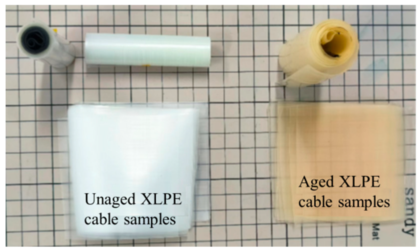
2.1. Sample Preparation

The cross-linked polyethylene (XLPE) insulation samples are obtained from a YJV62 single-core cable with a rated voltage of 10 kV, produced by Jinda Cable from Tianjin, China. The XLPE samples are made by a numerically controlled machine tool via ring cutting. All the samples have a thickness of 0.2 mm, as shown in Figure 1. A portion of the un-aged cable insulation layer from the middle section was ring-sectioned to obtain cable insulation slice samples. The obtained XLPE cable insulation material slices and remaining un-aged cable sections were subjected to thermal ageing in an oven. The acceleration temperature range is usually set between 120 and 140 °C, as it is found that a higher temperature may melt the XLPE sample and a lower temperature will not effectively accelerate the ageing process. So, we choose to use 135 °C as the accelerating temperature [9]. The cables were thermally aged for 0, 3, and 5 weeks. The aged cables were sectioned to obtain slices of the aged cable insulation material, which were labelled according to the ageing weeks, as AS0, AS3, AS5, etc.

The ring-sectioned cable slices are inherently curved, uneven, and marked with cutting scratches, which adversely affect the accuracy of experimental measurements. To obtain transparent and flat slice samples, the cable slices were placed in a 0.2 mm thick stainless-steel mould, with silicone oil-coated PET films placed on both the top and bottom surfaces to prevent adhesion. After heating the flat-plate vulcanizing press to 120 °C, the samples were placed inside and pressed under a pressure of 15 MPa for 40 s. Upon removal, they were sandwiched between water-cooled plates for cooling.

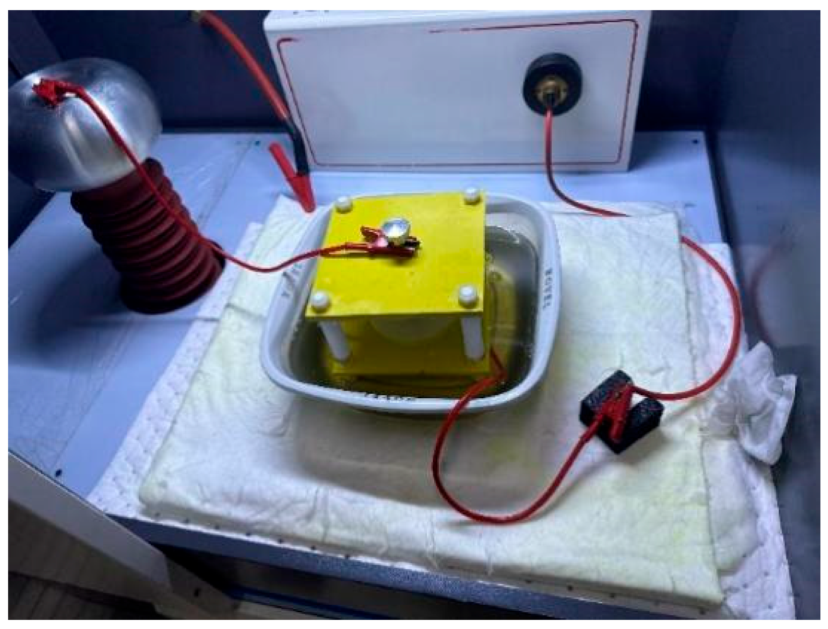
2.2. Accelerated-Ageing Test Platform

Acquisition of ageing lifetime exponents or other critical parameters for insulation material lifetime models necessitates accelerated-ageing tests, which predominantly employ the constant voltage method and step-up voltage method—each offering distinct advantages suited to different testing scenarios. The constant voltage method applies a steady voltage until specimen breakdown, providing simplicity and reliability but requiring extended test durations with inherent limitations including time inefficiency, low data acquisition rates under low-voltage conditions, and significant data dispersion. In contrast, the step-up voltage method, grounded in the cumulative ageing lifetime model, operates on the premise of irreversible ageing damage accumulation in insulation materials. This approach demonstrates superior efficiency, shorter testing cycles, and reduced data scatter. By incrementally elevating the applied voltage at predetermined time-steps until breakdown occurs, this method capitalizes on the cumulative effects inherent to solid insulation, particularly effective for materials lacking self-healing properties.

The Nelson model postulates that material residual lifetime is determined by the synergistic effects of voltage stress and breakdown probability at corresponding stress levels [10]. By conceptualizing insulation breakdown as a consequence of voltage stress accumulation, progressive voltage escalation enables evaluation of solid insulation’s endurance capability and remaining service life.

Figure 2 schematically illustrates the step-up voltage ageing test configuration with the following definitions:

V_s: Initial voltage;

T_r: Time step duration;

V_r: Voltage increment per step;

V_f: Breakdown voltage;

T_f: Final step duration.

In accelerated-ageing tests the prepared sheet samples are cleaned with alcohol and placed between the upper and lower electrodes, ensuring the samples are fully immersed in insulating oil. First, a constant voltage breakdown test is conducted at room temperature to determine the sample’s breakdown voltage range. For the step-stress method, the initial voltage is typically set to 60% of the room-temperature breakdown voltage [11]. The voltage gradient is selected to ensure at least three test steps before breakdown occurs, with gradient time intervals (e.g., 5 min, 10 min, 30 min) chosen. Voltage is continuously increased until the sample breaks down, and the breakdown time and voltage are recorded. The accelerated-ageing test setup is illustrated in Figure 3. In this study, the initial voltage was set to 45 kV, the voltage gradient to 5 kV, and three time-steps of 200 s, 600 s, and 1800 s were applied. The temperature is 25 °C, and the humidity is about 40%. To ensure the accuracy of the test, 6 samples are used in each group to reduce the dispersity of the data.

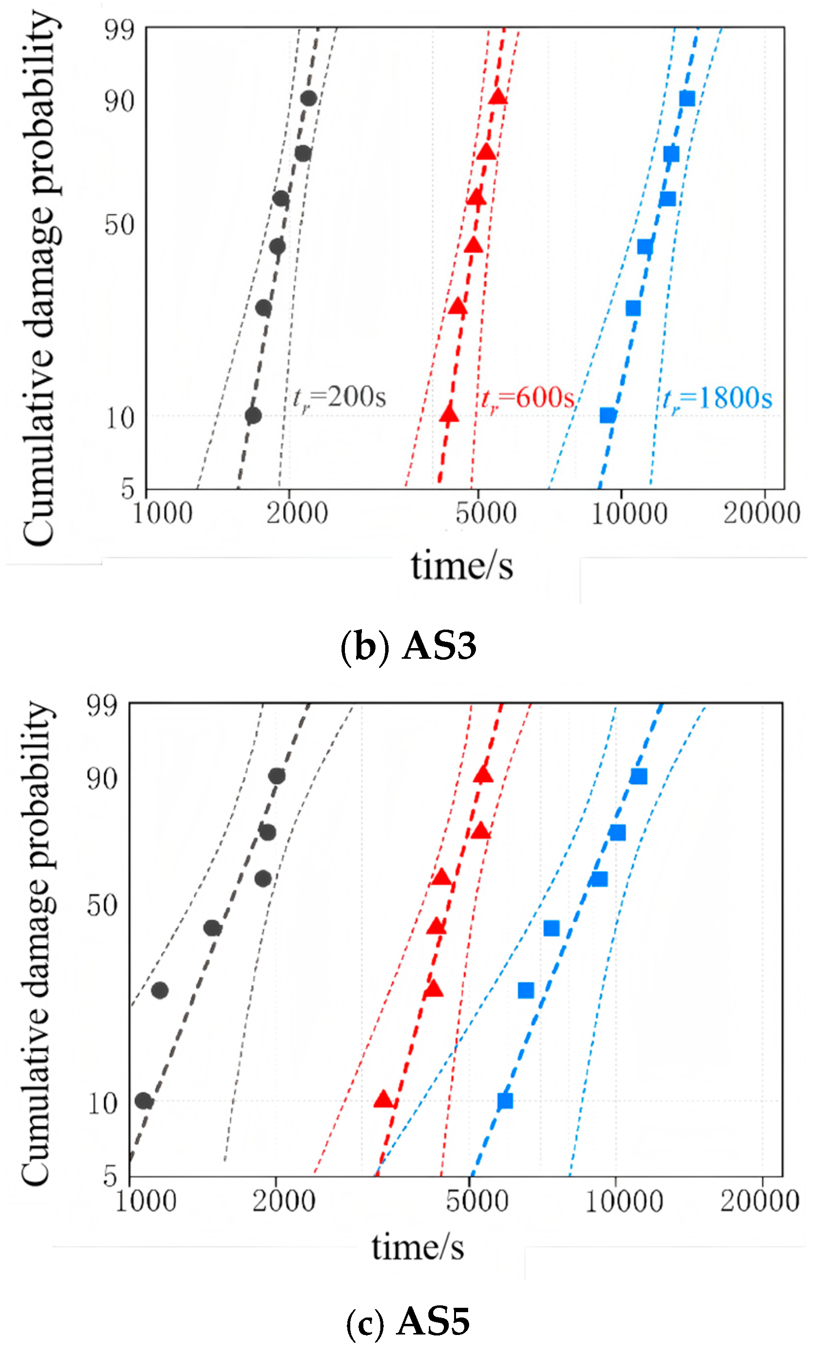
3. Measurement Results

The step-up voltage accelerated-ageing test was performed on aged cable insulation sheet samples to record the time required for the voltage level to incrementally increase from the initial voltage according to predefined time-steps until breakdown occurred. The results are shown in

Table 1. Gradual voltage rise test data of cable slices in different ageing states.

Sample	Step Duration (s)	No.	Breakdown Voltage (kV)	Total Time (s)	Last Step Time (s)
AS0	200	1	95	2135	90
		2	85	1678	33
		3	90	1920	75
		4	95	2194	149
		5	90	1887	42
		6	85	1762	117
	600	1	80	4519	274
		2	85	4884	39
		3	85	4954	109
		4	80	4337	92
		5	90	5494	49
		6	85	5191	346
	1800	1	80	12,696	51
		2	80	13,725	1080
		3	75	11,186	341
		4	90	12,509	1664
		5	65	10,546	1501
		6	70	9327	282
AS3	200	1	75	1374	129
		2	90	2017	172
		3	95	2187	142
		4	85	1783	138
		5	80	1461	16
		6	85	1679	34
	600	1	90	5459	14
		2	80	4399	154
		3	80	4505	260
		4	80	4336	91
		5	70	3446	401
		6	80	4519	274
	1800	1	70	10,832	1787
		2	65	8100	855
		3	65	8933	1688
		4	80	12,723	78
		5	75	11,645	800
		6	75	11,420	575
AS5	200	1	80	1474	29
		2	80	1550	105
		3	70	1106	61
		4	85	1768	123
		5	80	1528	83
		6	90	1935	90
	600	1	70	3167	122
		2	80	4273	28
		3	65	2522	77
		4	60	1993	148
		5	90	5801	356
		6	85	5165	320
	1800	1	70	9117	72
		2	75	10,873	28
		3	75	11,768	728
		4	65	7381	136
		5	70	9195	150
		6	65	7956	711

.

When the number of samples in the step-up voltage test is sufficiently large, the total breakdown time can be assumed to follow a Weibull distribution. Figure 4 illustrates the Weibull distribution of breakdown times for XLPE cable slices subjected to step-up voltage ageing tests under different time-steps. In the statistical analysis a confidence level of 0.95 was set. Additionally, the scale parameter of the Weibull distribution is defined as the characteristic ageing time, representing the typical time at which the material is likely to reach breakdown under specific conditions. Using the characteristic ageing times obtained from each experimental group, the corresponding characteristic breakdown voltages were further determined.

Table 2. Weibull distribution parameters of cable slices in different ageing states.

Sample	Step Duration (s)	Characteristic Breakdown Voltage (kV)	Characteristic Ageing Time (s)	Last Step Time (s)
Un-aged	200	90	2015	170
	600	85	5077	232
	1800	75	12,308	1463
AS3	200	90	1874	29
	600	80	4701	456
	1800	75	11,284	439
AS5	200	85	1697	52
	600	80	4290	45
	1800	70	10,539	1194

presents the Weibull distribution parameters of XLPE sheet samples with different ageing degrees under three step durations. The results show that the characteristic breakdown voltage of the same sample decreases with increasing step duration. Under a fixed step duration, XLPE sheet samples with prolonged ageing time exhibited lower characteristic breakdown voltages.

4. Analysis

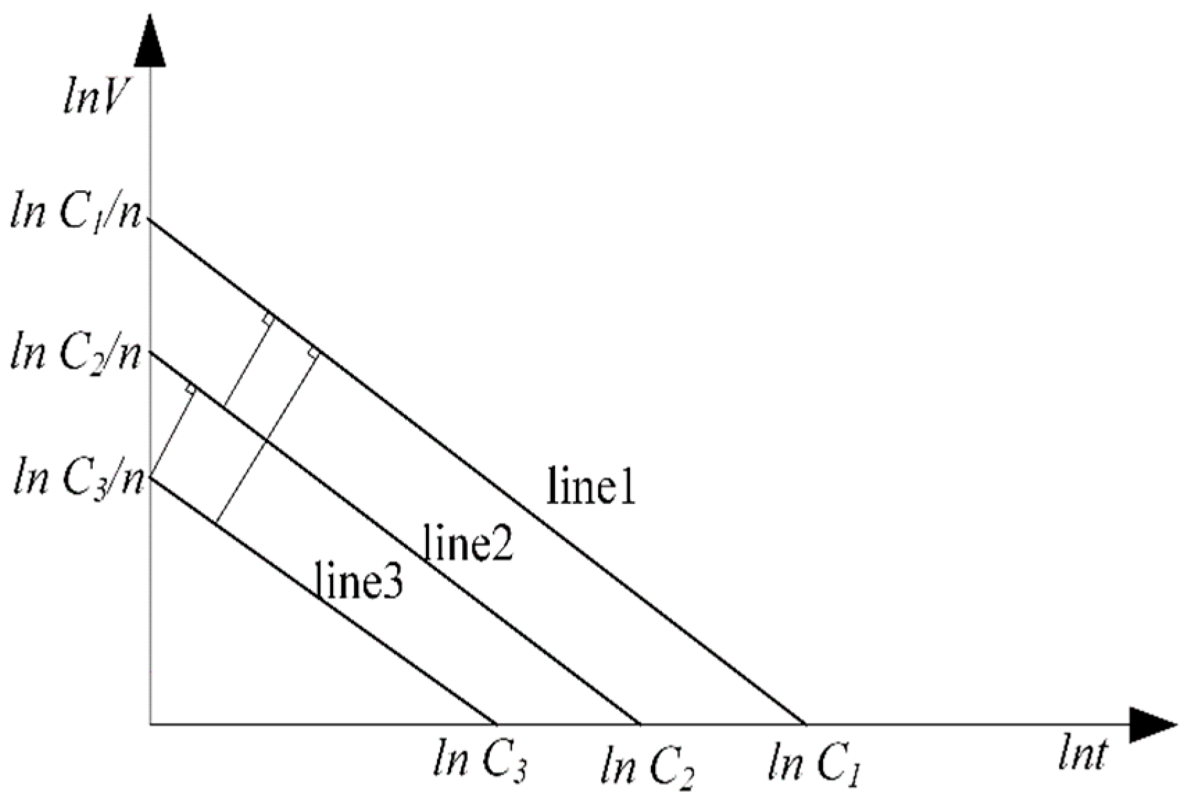
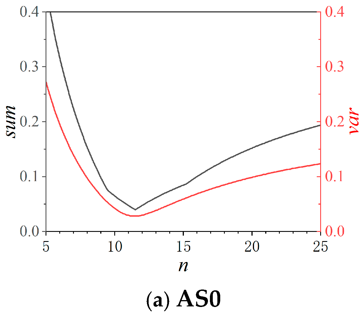
4.1. Insulation Ageing Lifetime Evaluation Based on Inverse Power Model

The inverse power model, which is the most widely used empirical model in engineering [11,12], can be used to estimate the electrical ageing life of materials. It is expressed by Formula (1) as follows:

$$t_2=t_1{\left({\displaystyle \frac{U_2}{U_1}}\right)}^n$$

(1)

where n is the ageing exponent of the inverse power model, t₁ is the electrical ageing life at U₁, and t₂ is the electrical ageing life at U₂.

Equation (1) can be expressed as follows:

$$C=U^{n}t$$

(2)

In the inverse power model, C is a constant, and the higher the applied voltage, the shorter the time required for insulation breakdown. Due to the uncertainty in insulation failure time, the ageing life also exhibits uncertainty. Consequently, the insulation breakdown time is treated as a probability function.

Equation (2) can be modified based on the step-up voltage test as follows:

$$C={\displaystyle \sum t_r{V}_i^n}+t_f{V}_f^n$$

(3)

where t_r is step duration/s; V_i is voltage level at each step/kV; t_f is final step time/kV; V_f is breakdown voltage/kV. It should be noted that the value of C is usually regarded as an accumulated ageing ‘amount’, however, its unit depends on the value of n and it actually has no real physical meaning.

To determine the lifetime exponent n, this study defines three step durations t_r1, t_r2, and t_r3, with the final step voltage levels set as V_f1, V_f2, and V_f3, and the final step times as t_f1, t_f2, and t_f3, Equation (3) can be reformulated as follows:

$$\left\{\begin{array}{c}{C}_1={\displaystyle \sum t_{r1}{V}_i^n}+t_{f1}{V}_{f1}^n\\ C_2={\displaystyle \sum t_{r2}{V}_i^n}+t_{f2}{V}_{f2}^n\\ C_3={\displaystyle \sum t_{r3}{V}_i^n}+t_{f3}{V}_{f3}^n\end{array}\right.$$

(4)

Since directly solving Equation (4) is challenging, the value of n is predefined to facilitate computation, and the ageing life accumulation parameter C is calculated with this preset value. By taking the logarithm of both sides, we obtain the following:

$$\left\{\begin{array}{c}\ln (C_1)=\ln (t_1)+n\ln (V_1)\\ \ln (C_2)=\ln (t_2)+n\ln (V_2)\\ \ln (C_3)=\ln (t_3)+n\ln (V_3)\end{array}\right.$$

(5)

According to Equation (5), three straight lines are plotted in the lnV-lnt coordinate system, as shown in Figure 5. These lines correspond to material ageing data under three different step durations. Assuming that they are under the same temperature condition, the data from these varying time intervals maintain consistency with their respective lifetime exponent n and the three lines are parallel to each other. If the ageing life accumulation parameter C differs for each step duration, the intercepts of each line with the coordinate axes will also vary. By defining the true value of the lifetime exponent as n₀, the ageing life accumulation parameter C should remain constant under this value, causing the three lines to coincide. However, due to experimental deviations and data uncertainty, it is generally impossible for the three curves to perfectly overlap. As the value of n gradually approaches the true n₀, the spacing between the curves continuously decreases. Thus, the n value that minimizes this spacing is considered the true lifetime exponent.

In Figure 5, the sum of the absolute values and the variance of the pairwise distances between the three straight lines can serve as criteria to determine whether the value of n has reached the true value. The distance between any two lines can be expressed by the following formula:

$$d_{12}=\cos {\alpha }_{12}\cdot \left|{\displaystyle \frac{\ln C_1}{n}}-{\displaystyle \frac{\ln C_2}{n}}\right|={\displaystyle \frac{\left|\ln C_1-\ln C_2\right|}{\sqrt{n^2+1}}}$$

(6)

The following formulas can be used to describe the sum of the distances between straight lines (denoted as sum) and the variance of the distances (denoted as var):

$$sum={\displaystyle \sum {\mathit{d}}_{\mathit{i}\mathit{j}}}$$

(7)

$$\mathrm{var}=\sqrt{{\displaystyle \sum {{\mathit{d}}_{\mathit{i}\mathit{j}}}^2}}$$

(8)

Within the range of 1–30, we select the n value that yields the lowest sum and var values as the true value.

The dependence of total inter-curve spacing and variance on the ageing lifetime exponent n in the inverse power model is demonstrated in Figure 6. It can be seen that the values of the sum and var all decrease first and then increase. There is a lowest point in the figure which is related to the true value of the ageing parameter of the IPM. So, the ageing parameters of samples with different ageing states can be calculated, and the specific data are listed in

Table 3. Inverse power model characteristic parameters.

	AS0	AS3	AS5
C1	1.6 × 1059	2.67 × 1059	9.74 × 1060
C2	1.13 × 1059	1.06 × 1060	9.56 × 1060
C3	1.69 × 1059	4.79 × 1059	1.04 × 1061
C	1.47 × 1059	6.2 × 1059	9.90 × 1060
n	11.5	11.7	12.1

.

It seems that the value of C increases with the ageing time. If it strictly reflects the accumulated ageing ‘amount’, it suggests that the sample with long ageing time can withstand a higher accumulated ageing ‘amount’ than the un-aged sample. This does not make sense as the sample with ageing history should have more accumulated ageing amount before the ageing test, and then the tested accumulated ageing ‘amount’ of the aged sample should be smaller than the un-aged sample. So, here there is a chaos of the physical links between the ageing process and the parameter of IPM.

It can also be seen that the ageing parameter of IPM n increases from 11.5 to 12.1 with the ageing process. Both the values of C and n determine the ageing life curve (the V-t plot), as shown in Figure 7. The ageing parameter n does not have a clear physical meaning, but it defines the slope of the lnV-lnt, where the bigger the n value the gentler the slope, as shown in Figure 7.

It can also be seen that the line for the un-aged sample is above the other lines, with a higher intercept at the Y axis. It shows that the un-aged sample has a higher breakdown voltage than the other samples. The intercept of the X axis at the voltage of 10 kV reflects the estimated lifetime of the sample. It can be seen that the un-aged sample has a longer estimated lifetime than the aged sample.

However, it still does not have a solid physical meaning which can directly link to the physics of the ageing process. And it can hardly explain why the n value increase and how it may link to the insulation property. And it should be noted that the value of C strongly depends on the value of n, as n is the index of V. That is why C cannot truly and strictly reflect the accumulative ageing ‘amount’. Both the values of n and C of IPM cannot be used as a parameter to reflect the ageing state of the insulation.

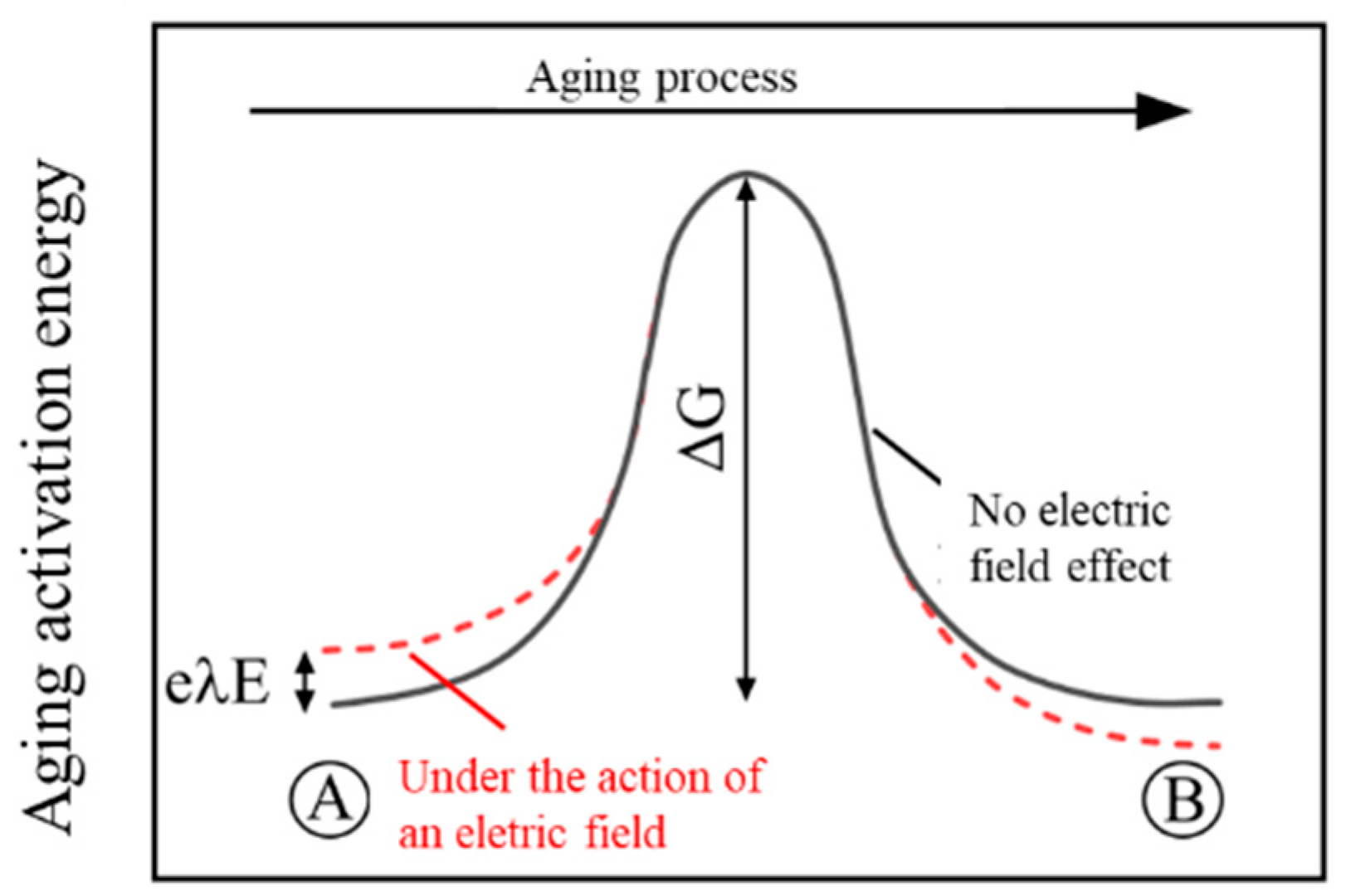
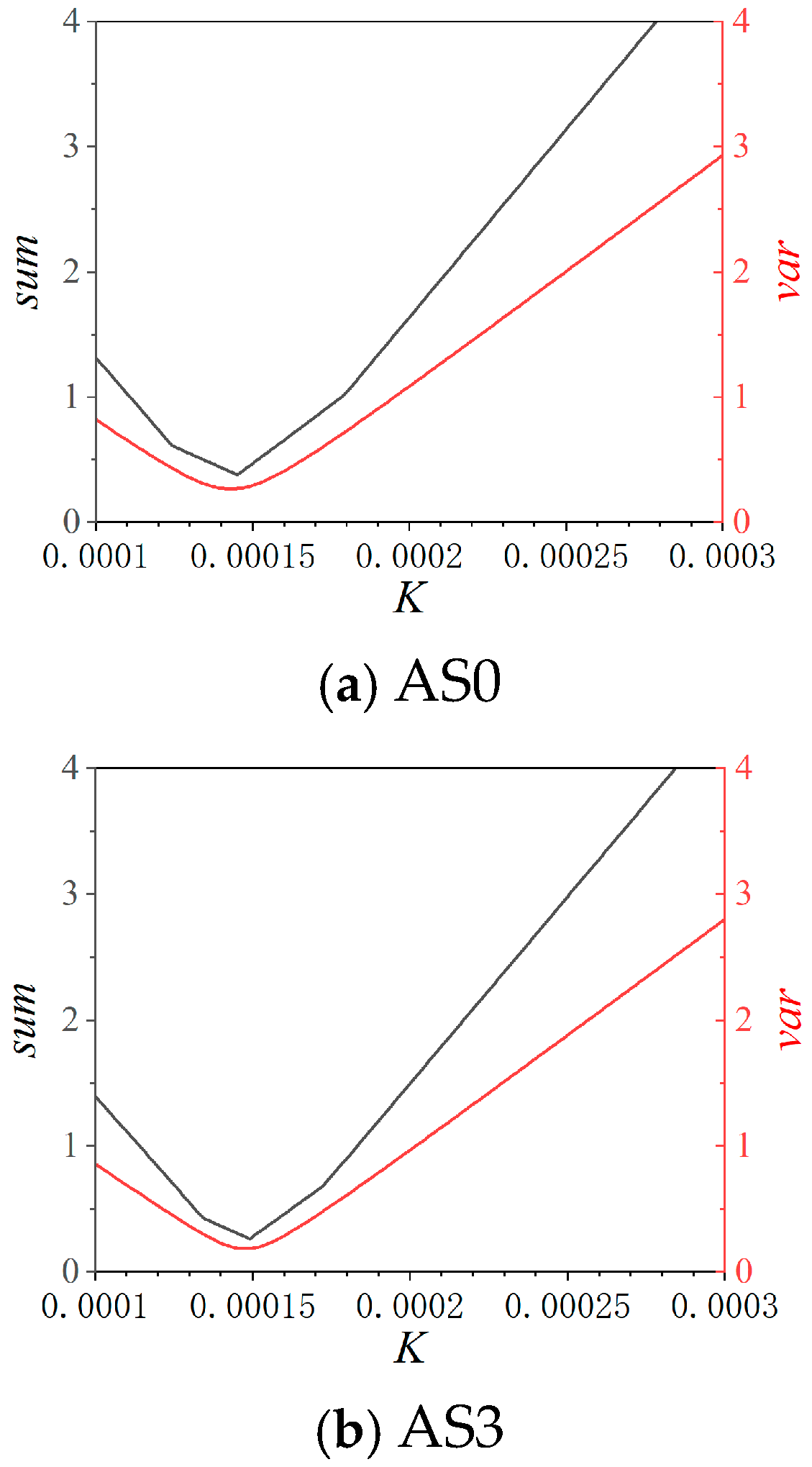
4.2. Insulation Ageing Lifetime Evaluation Based on Crine’s Model

The Crine model assumes that polymer ageing is a thermally activated process requiring the overcoming of a free energy barrier, as shown in Figure 8. It considers that the microcavity or free volume is the origin position of the ageing. The ageing happens when the electrons in the free volume obtain higher energy than the ageing activation energy barrier ΔG₀ and break the chain of polymer to make a bigger defect. The applied electric field will increase the energy of the free electrons with an acceleration distance λ. In the assumption of the Crine model, λ is limited by and equal to the maximum length of microcavities or free volume. The variation in activation energy barrier correlates with the material’s initial and final free energy states and is influenced by van der Waals bond strength. When the electric field-induced change in activation energy exceeds the interbond cohesive energy, bond rupture occurs. Above the critical field strength, the charges in microcavities have big enough energy to break the chemical chain of the material, leading to a reduction in the insulation property.

The Crine model formula under high field strength can be expressed as follows:

$$\mathit{t}\approx {\displaystyle \frac{h}{2kT}}{e}^{{\displaystyle \frac{\Delta G_0-e\lambda E}{kT}}}$$

(9)

where T is the absolute temperature/K; k is the Boltzmann constant; h is the Planck constant; E is the electric field strength/V·m⁻¹; ΔG₀ is the activation energy of ageing/eV; and λ is the acceleration distance equal to the maximum length of microcavities or free volume in XLPE/m.

Under constant temperature conditions it is assumed that λ and ΔG₀ remain unchanged. Let $K={\displaystyle \frac{e\lambda }{kTd}}$ and ${L={\displaystyle \frac{h}{2kT}}e}^{{\displaystyle \frac{∆G_0}{kT}}}$, which can be considered constants. Equation (9) is rewritten in the following exponential form:

Note: The placeholders “K = ${\displaystyle \frac{e\lambda }{kTd}}$” and “L = ${\displaystyle \frac{h}{2kT}}{e}^{{\displaystyle \frac{∆G_0}{kT}}}$” are retained as in the original text, likely indicating that specific expressions for K and L were omitted.

$${\mathit{t}\mathit{e}}^{KU}=L$$

(10)

where L can be regarded as a parameter quantifies the accumulative degradation due to ageing. Then, set the test parameters to be consistent with calculating the ageing parameter of the inverse power model. According to the step-stress, Equation (10) can be written in the following form:

$$L={\displaystyle \sum t_i{e}^{k{U}_i}+t_f{e}^{K{U}_f}}$$

(11)

where similarly to solving the problem of the ageing parameter for the inverse power model, the values of K are firstly set in a range. And then the values of sum and var for different K values can be calculation. Then the true value of K can be determined when both sum and var are with minimum value. Tests conducted over a wide range show that the true value generally falls within the range of 0.0001 to 0.001. Figure 9 illustrates the variation in the sum and var values with the ageing parameter K for XLPE cable insulation sheet samples at room temperature based on the Crine model.

It can be seen that the values of K decrease first and then increase. It is similar to the condition of Figure 6. The lowest point of K corresponds to the condition in which the three sets of data have the smallest dispersity and is with the true values. Substituting the obtained K and L values into the equation allows for the calculation of acceleration distance λ and ageing activation energy barrier ΔG₀, with the results presented in

Table 4. The feature parameters of the Crine model.

	AS0	AS3	AS5
K	0.000145	0.000149	0.00016
L1	1.66 × 108	1.40 × 108	1.49 × 108
L2	1.79 × 108	1.50 × 108	1.93 × 108
L3	1.65 × 108	1.46 × 108	1.93 × 108
L	1.7 × 108	1.45 × 108	1.78 × 108
ΔG0 (eV)	1.269	1.265	1.27
λ (m)	0.739 × 10−9	0.753 × 10−9	0.809 × 10−9

.

As shown in Table 4, the ageing activation energy ΔG₀ shows very small variation with the different ageing states. The biggest error between the values of ΔG₀ is just 0.4%. It shows that the ageing activation energy ΔG₀ does not change with the ageing process and can be considered as a material intrinsic parameter. The value of the ageing activation energy ΔG₀ may corresponds to the bond energy of PE chain, the cross-linking network, and the band energy of the XLPE insulation. However, more work is still needed to reveal this detailed relationship.

λ is the acceleration distance of the free electron, and equals the maximum length of microcavities or free volume. Table 4 demonstrates that as ageing time increases, the value of λ increases, leading to greater electron acceleration distances within the microcavities or free volume. It consequently makes the electrons with higher energy more likely to cause damage on XLPE chains. Then the lifetime of the aged sample becomes shorter than the un-aged sample. The test results also make sense as the ageing process may break the polymer chain of XLPE, and make larger sized microcavities or free volume. So the value of the acceleration distance can be regarded as an indicator for the estimation of the insulation lifetime. In the case of unchanged ageing activation energy, the bigger the acceleration distance, the shorter the insulation lifetime.

The ageing lifetime curve based on the Crine model is shown in Figure 10. It can be seen that the ageing lifetime gradually decreases with increasing ageing time, and the remaining lifetime of aged specimens is significantly shorter than that of un-aged specimens. The result is similar to the trend of the IPM, but still has some differences.

The first difference is that the slope of lnV-lnt changes in the ageing life curve based on the Crine model rather than the IPM. The reason is that the higher the electric field, the higher energy the electrons are supposed to observe from the electric field. And then the electrons are more probable to cause damage to the sample in the higher electric field than in the lower electric field. However, due to the existence of the activation energy, it behaves differently with the IPM. When the lifetime is very short, the voltage should be very near to the breakdown voltage. It is more reliable for the Crine model, as the voltage changes slightly with the lifetime when the lifetime is shorter than 10 s. But the IPM suggests that the voltage may continuously increase as there is a decrease in the lifetime. It does not make sense. Similarly, when the voltage is very low, the lifetime of insulation based on the Crine model tends to reach a maximum value rather than continuously increase, as suggested by the IPM. This is also due to the limited activation energy. The electrons cannot only obtain energy from electric field but also from the thermal kinetic activities. They still have a very small possibility to cause damage in the condition of limited activation energy. So, the Crine model describes a more reasonable lifetime trend than the IPM.

The second difference is that the Crine model predict a much shorter lifetime than the IPM at the voltage of 10 kV. The 5 weeks aged samples have about 1.29 years remaining lifetime in the Crine model, while they have a 142,694 years lifetime in the IPM. Even though it is in the condition of room temperature, it is still inaccurate that the 5 weeks aged sample has such a long remaining lifetime. However, it is still hard to clearly figure out which prediction is more reliable, as the long-term test has many factors which are hard to control and takes too much time and cost.

With the discussions above, it can be seen that the key parameters of the Crine model have clear physical meaning, while the IPM can only fit the mathematic pattern of the data. The activation energy barrier of the Crine model does not change with the ageing process, so that it can be considered as a material intrinsic parameter that is determined by the nature of the bond, cross-linking network, and band energy of the XLPE. The acceleration distance of the Crine model increases with the ageing time, so it can be regarded as an indicator of the ageing state. Conversely, the key parameters of the IPM do not have clear physical meaning and their change with ageing time cannot be sufficiently used as an indicator of ageing states. Furthermore, the Crine model describes a more reasonable ageing lifetime pattern than the IPM, especially when the voltage is high and low. So, the Crine model has a greater potential to be used in the remaining lifetime estimation of the cable insulation or other materials.

5. Conclusions

This paper tests the remaining lifetime of aged and un-aged XLPE samples with the step-stress method. The inverse power model and the physical-driven Crine model are employed in the analysis, and the calculation method of the key parameters of the two models are proposed. The characteristics of remaining lifetime and key ageing parameters of the samples with different ageing states are discussed regarding the two models. The following conclusions are drawn:

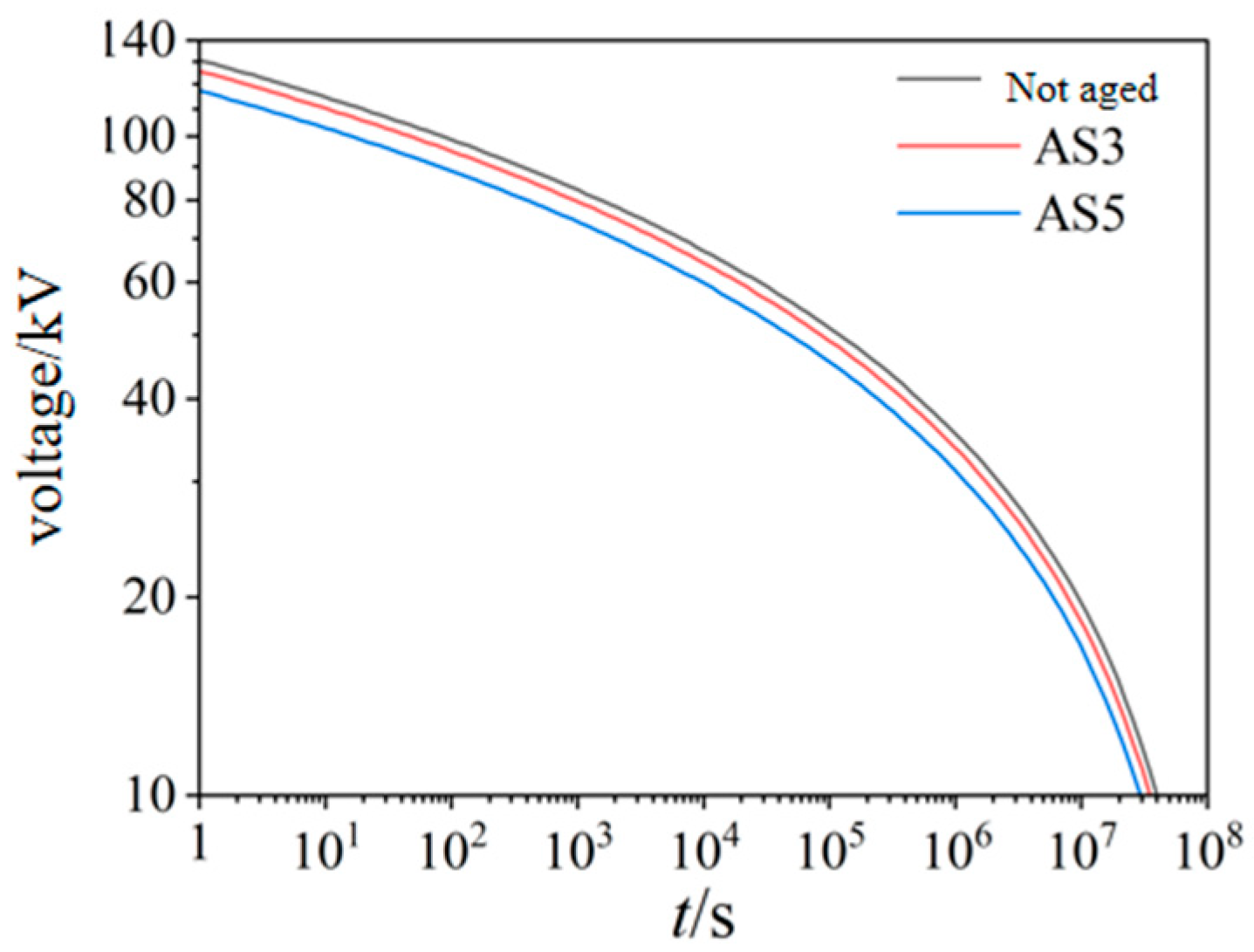
• The step-stress method can efficiently obtain the lifetime data of the insulation samples. It is found that the longer the ageing time, the shorter the remaining lifetime of the XLPE sample.
• The ageing parameters n and C of the IPM increase with the ageing time, but they can hardly link to the physics of the ageing process, and they cannot be used as an indicator of the ageing state.
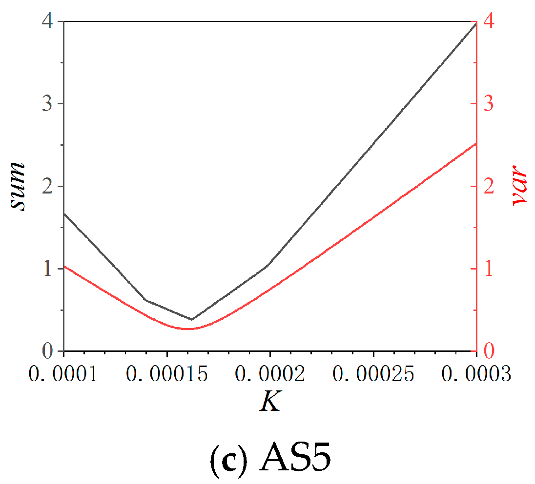
• The activation energy barrier of the Crine model does not change with the ageing process, and so it can be considered as a material intrinsic parameter determined by the material nature. The acceleration distance of the Crine model increases with the ageing time, and it can be regarded as an indicator of the ageing state.
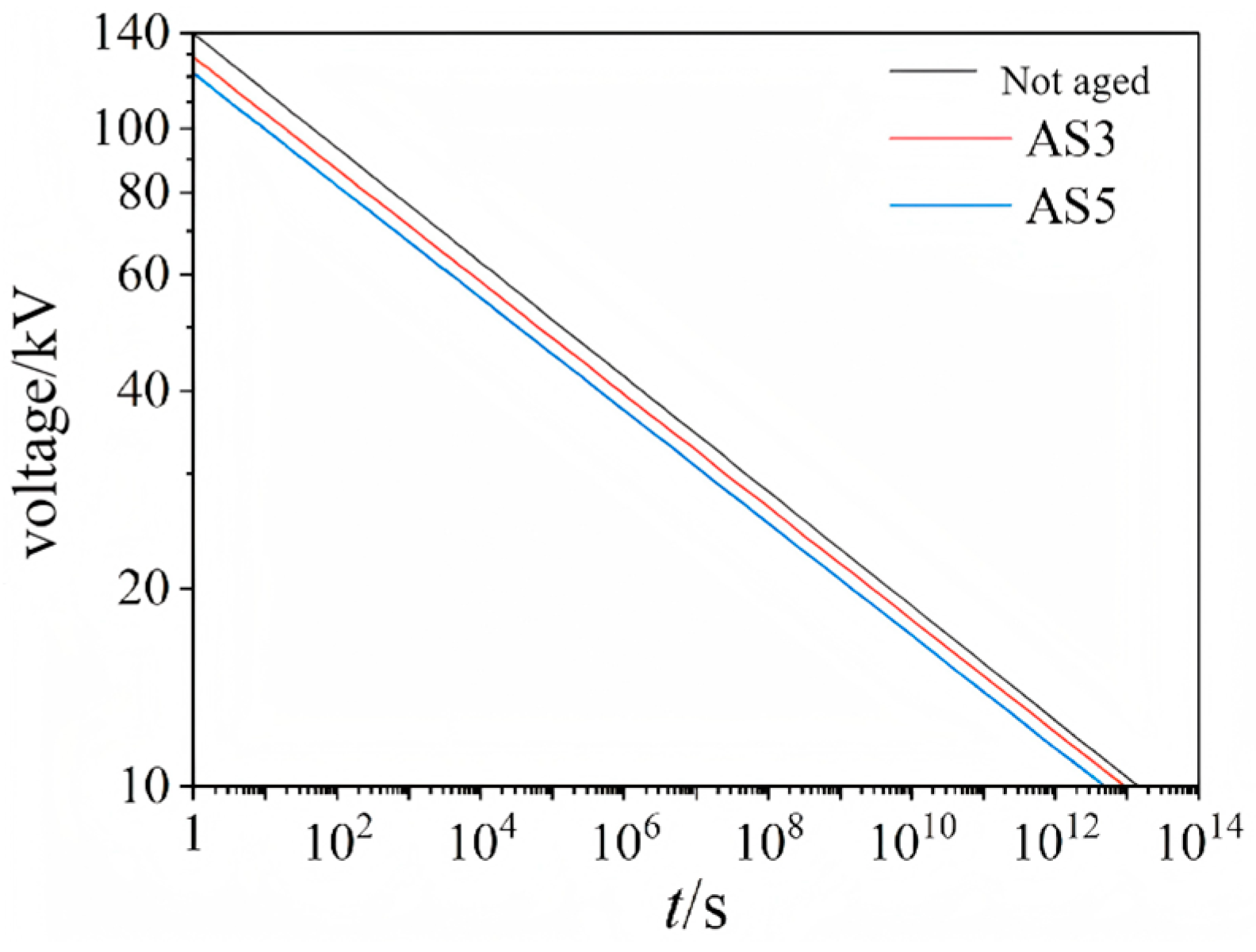
• The Crine model describes a more reasonable ageing lifetime pattern than IPM, especially when the voltage is high and low. The Crine model has a greater potential to be used in the remaining lifetime estimation of the cable insulation or other materials.

References

1. Du, B.X.; Li, Z.L.; Yang, Z.R.; Li, J. Application and Research Progress of HVDC Cross-Linked Polyethylene Cables. High Volt. Eng. 2017, 43, 344–354. [Google Scholar]
2. Zhou, T.X.; Wang, L.Y.; Ji, X.P.; Han, X.Y. Power Grid Scale Prediction and Optimization Needs Based on Policy Requirements of Modern Infrastructure System. Electr. Power 2024, 57, 1–8. [Google Scholar]
3. China Electricity Council. Annual Development Report of China’s Electric Power Industry 2019; China Building Materials Industry Press: Beijing, China, 2019. [Google Scholar]
4. Dakin, T.W.; Studniarz, S.A. The voltage endurance of cast and molded resins. In Proceedings of the 1977 EIC 13th Electrical/Electronics Insulation Conference, Chicago, LI, USA, 25–29 September 1977. [Google Scholar]
5. Endicott, H.S.; Hatch, B.D.; Sohmer, R.G. Application of the eyring model to capacitor ageing data. IEEE Trans. Compon. Parts 1965, 12, 34–41. [Google Scholar] [CrossRef]
6. Lewis, T.J.; Liewellyn, J.P.; Freestone, J.; Hampton, R.N. A newmodel for electrical ageing and breakdown in dielectrics. In Proceedings of the Seventh International Conference on Dielectric Materials, Measurements and Applications, IET, Bath, UK, 23–26 September 1996. [Google Scholar]
7. Dissado, L.; Mazzanti, G.; Montanari, G.C. The incorporation of space charge degradation in the life model for electrical insulating materials. IEEE Trans. Dielectr. Electr. Insul. 1995, 2, 1147–1158. [Google Scholar] [CrossRef]
8. Crine, J.P.; Parpal, J.L.; Lessard, G. A model of ageing of di-electric extruded cables. In Proceeding of the 3rd International Conference on Conduction and Breakdown in Solid Dielectrics, Trondheim, Norway, 3–6 July 1989. [Google Scholar]
9. GB/T 11026.1-2012; National Standard of the People’s Republic of China. Electrical Insulating Materials—Thermal Endurance—Part 1: Ageing Procedures and Evaluation of Test Results. General Administration of Quality Supervision, Inspection and Quarantine of the People’s Republic of China and the Standardization Administration of the People’s Republic of China: Beijing, China, 2012.
10. Zhang, Z.; Li, Y.; Zheng, Y.; Li, H.; Zhao, X.; Li, B.; Pei, X.; Cheng, Y. Insulation Aging Assessment Method for HVDC Cable Based on Space Charge Characteristics. Guangdong Electr. Power 2019, 32, 98–105. [Google Scholar]
11. Wang, Y.; Lv, Z.; Wang, X.; Wu, K.; Zhang, C.; Li, W.; Dissado, L.A. Estimating the inverse power law aging exponent for the DC aging of XLPE and its nanocomposites at different temperatures. IEEE Trans. Dielectr. Electr. Insul. 2016, 23, 3504–3513. [Google Scholar]
12. Xia, W.; Xiaotong, S.; Quanyu, L.; Wu, K.; Tu, D. Research progress on insulation ageing life model based on space charge effect. High Volt. Eng. 2016, 42, 861–867. [Google Scholar]
Figure 1. XLPE cable insulation slice sample.
Energies 18 03179 g001
Figure 2. Schematic diagram of gradually increasing pressure method for accelerating ageing test pressure.
Energies 18 03179 g002
Figure 3. Step-stress method accelerated ageing test pressure test diagram.
Energies 18 03179 g003
Figure 4. Distribution of breakdown time for XLPE sheet specimens (Black: tr = 200 s, Red: tr = 600 s, Blue: tr = 1800 s).
Energies 18 03179 g004aEnergies 18 03179 g004b
Figure 5. Data analysis in lnV-lnt coordinate system.
Energies 18 03179 g005
Figure 6. The variation in sum (black line) and var (red line) values of XLPE cable insulation sheet pattern with n value.
Energies 18 03179 g006aEnergies 18 03179 g006b
Figure 7. The ageing life curve of samples with different ageing states based on the inverse power model.
Energies 18 03179 g007
Figure 8. The diagram of the ageing process of the Crine model.
Energies 18 03179 g008
Figure 9. The variation in sum (black line) and var (red line) values of XLPE cable insulation sheet pattern with K value.
Energies 18 03179 g009aEnergies 18 03179 g009b
Figure 10. The ageing life curve of samples with different ageing states based on the Crine model.
Energies 18 03179 g010