
Comprehensive Performance Assessment of Conventional and Sequential Predictive Control for Grid-Tied NPC Inverters: A Hardware-in-the-Loop Study

 , ,
, ,  , , and
Abstract
1. Introduction
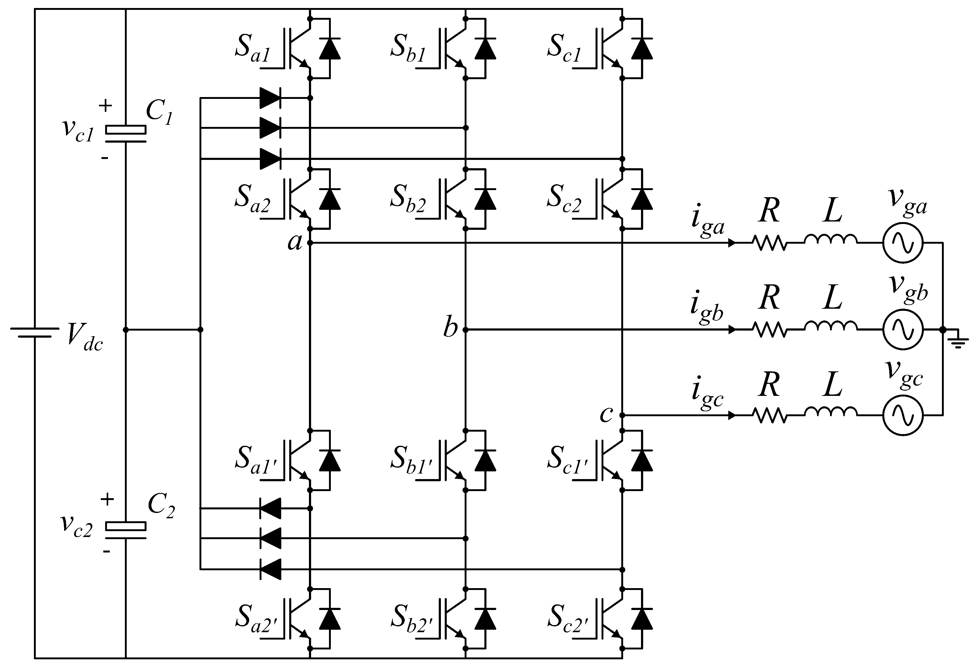
2. System Modelling
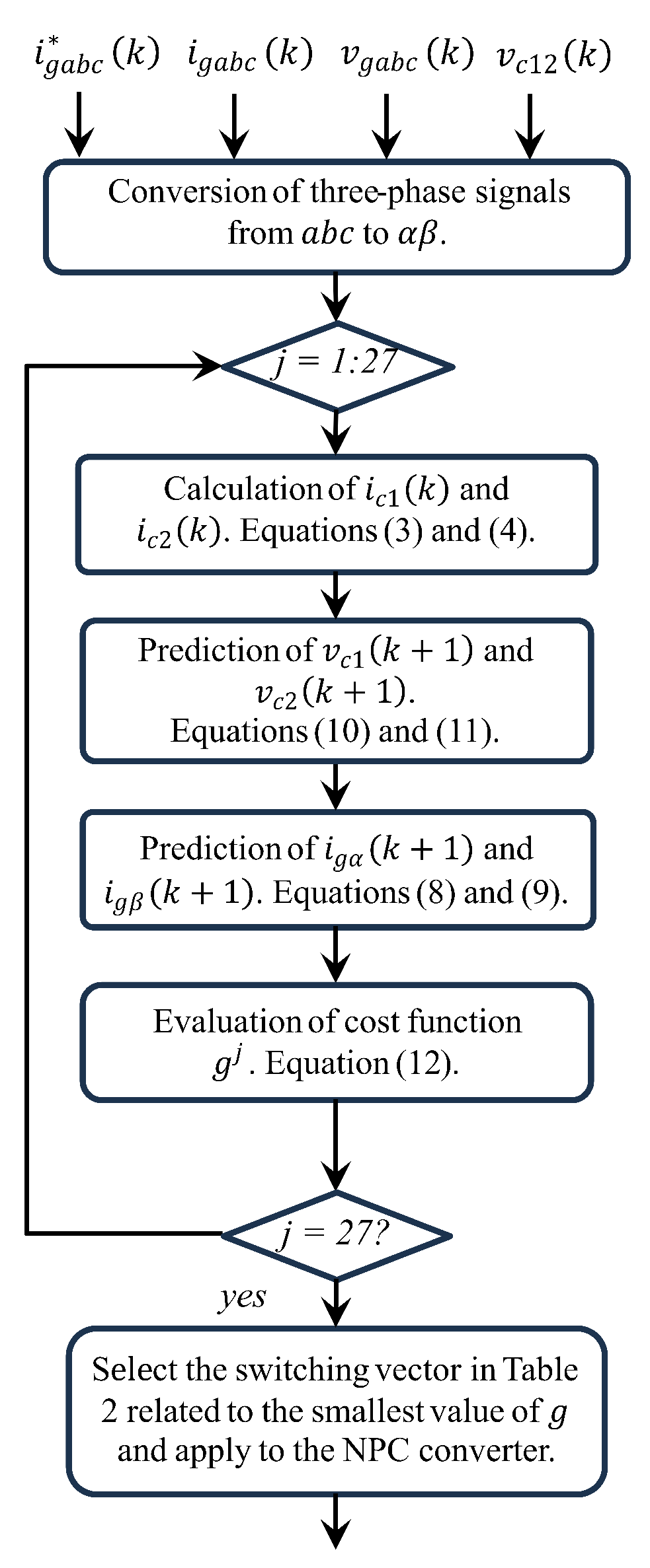
2.1. Conventional Model Predictive Control (C-MPC)
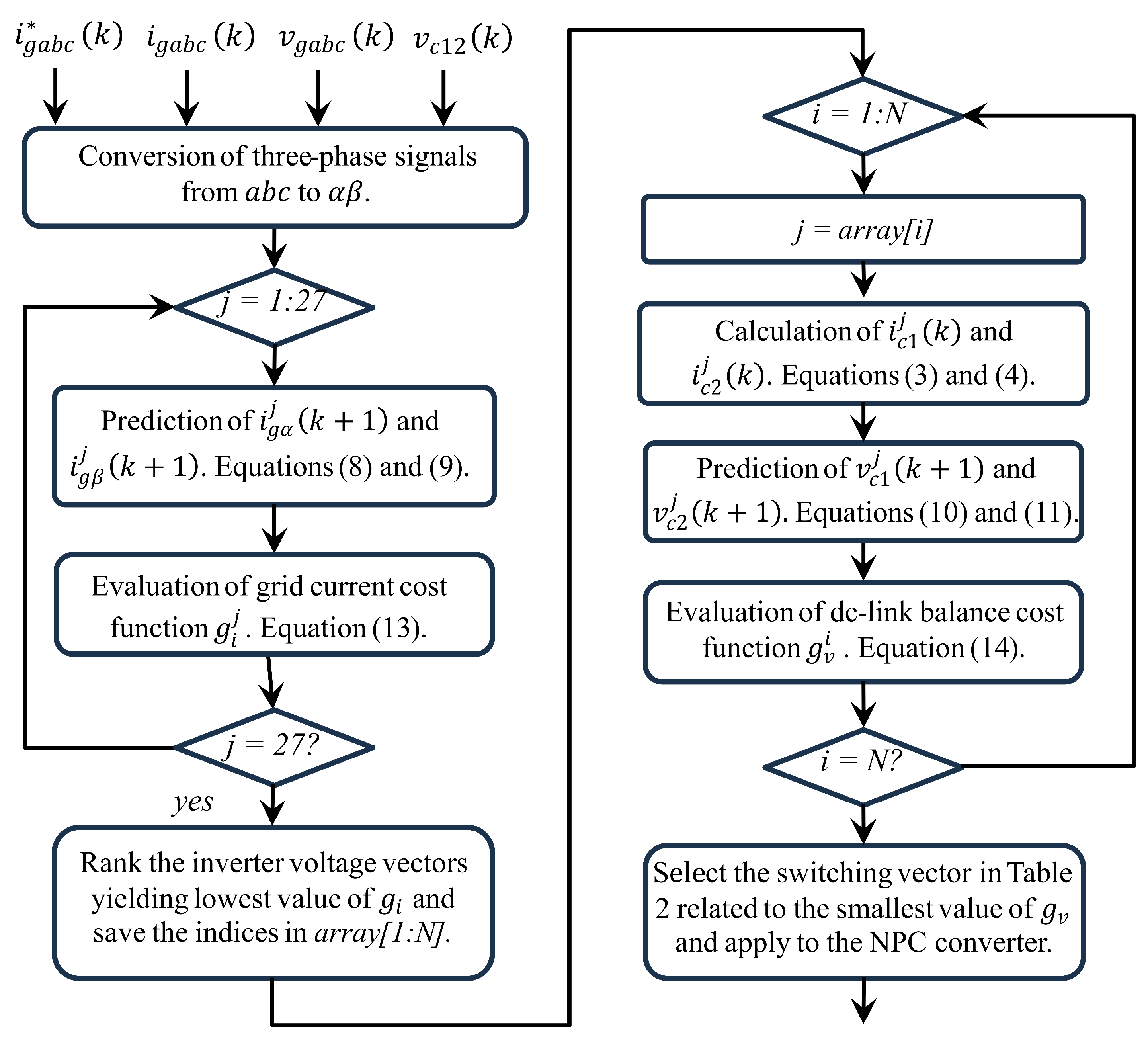
2.2. Sequential Model Predictive Control (S-MPC)
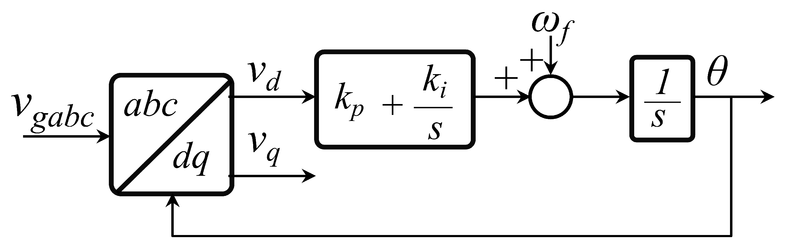
2.3. Current Reference Generation (PLL Design)
3. Determination of MPC Parameters
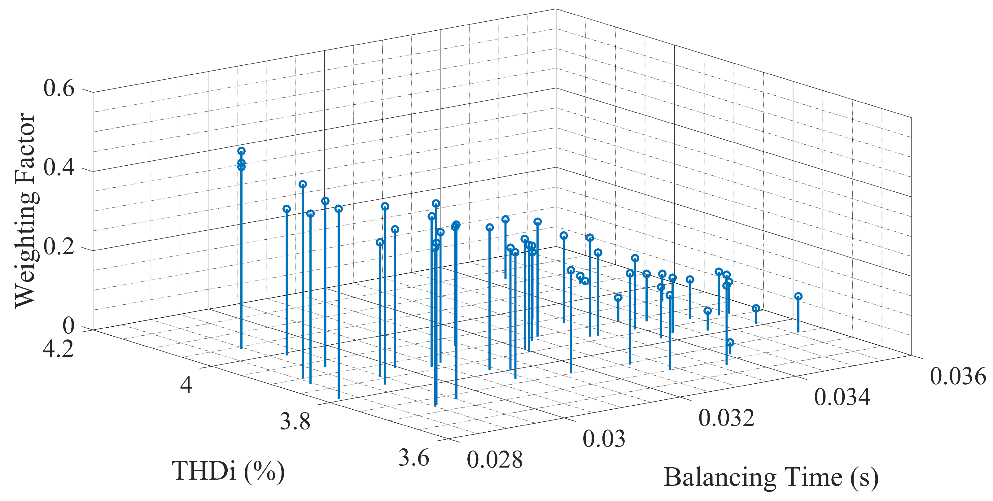
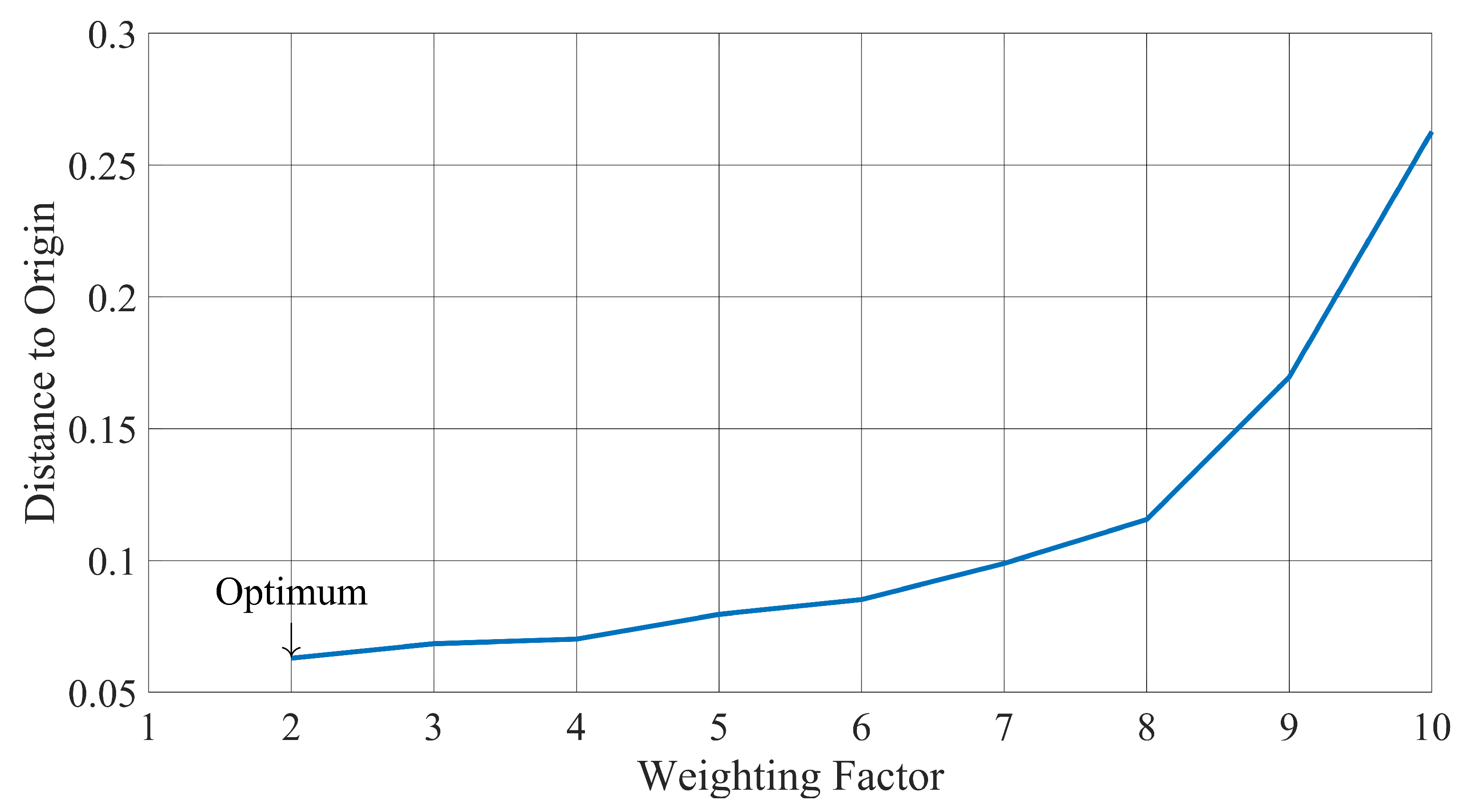
3.1. Optimal for C-MPC Strategy
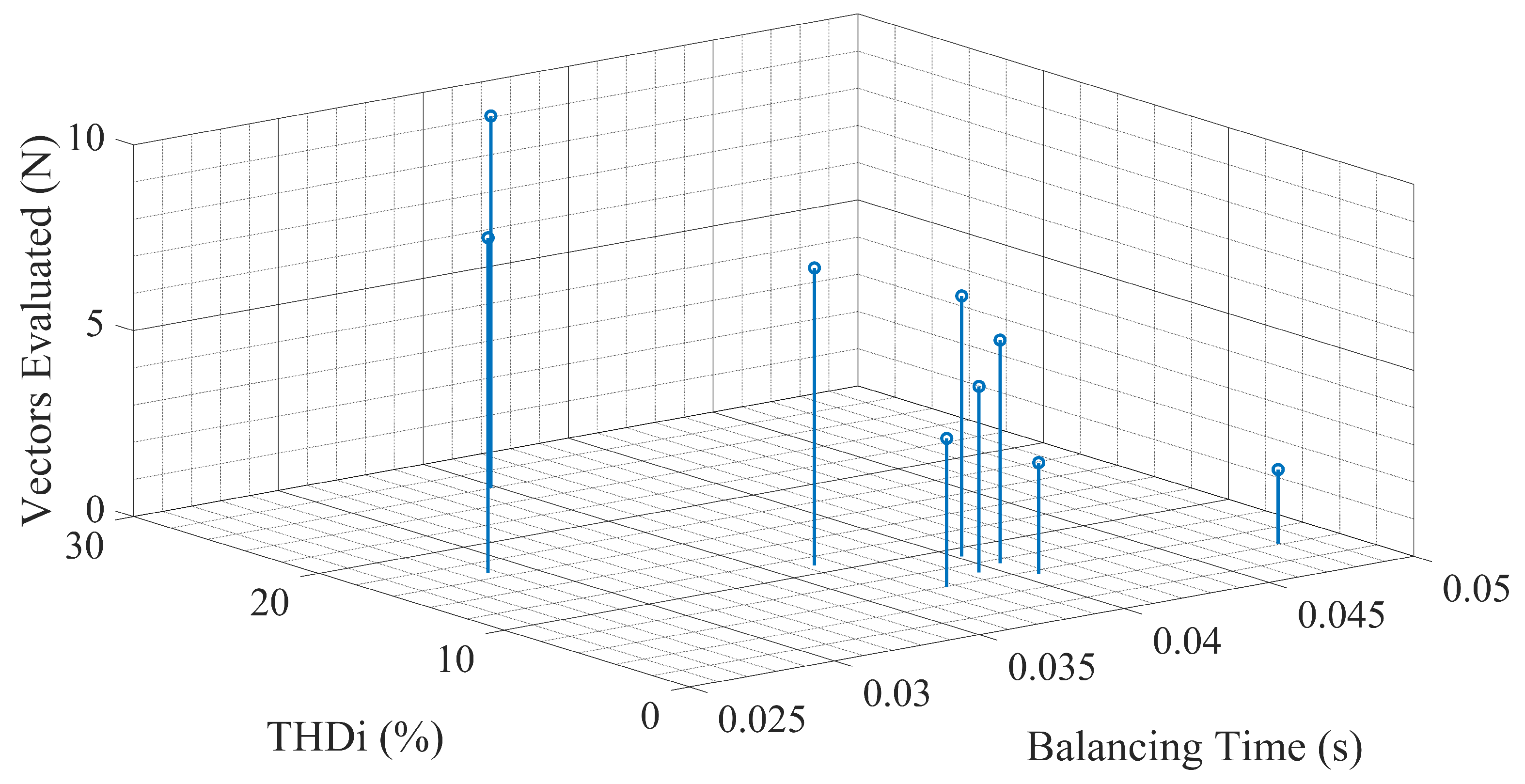
3.2. Optimum Number of Candidates Voltage Vectors for S-MPC Strategy
4. Hardware in the Loop (HIL) Implementation
4.1. Design of NPC Inverter Parameters
4.2. Real-Time HIL Overview
4.3. Working Flow
5. Results Analysis
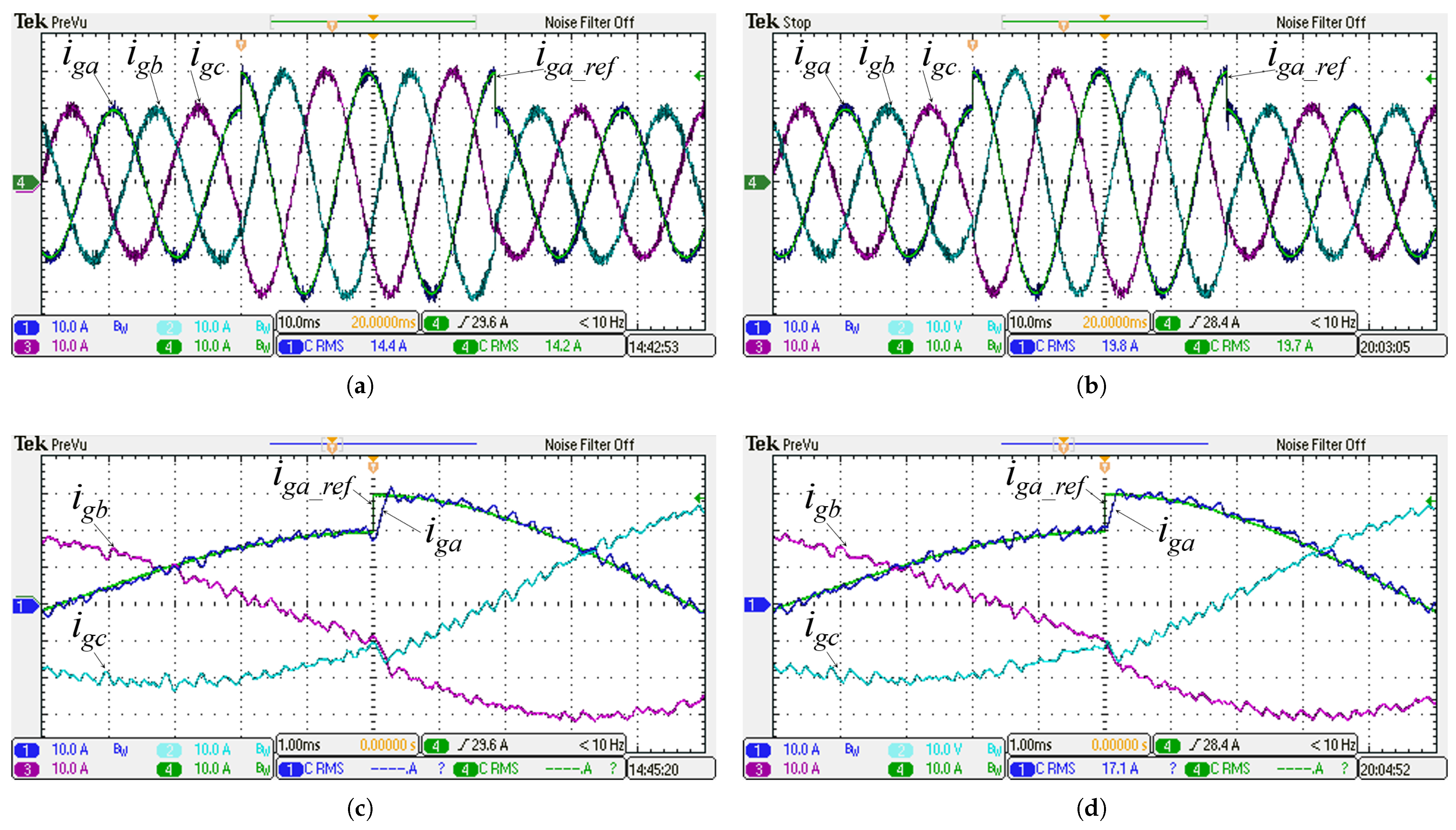
5.1. Steady-State Response
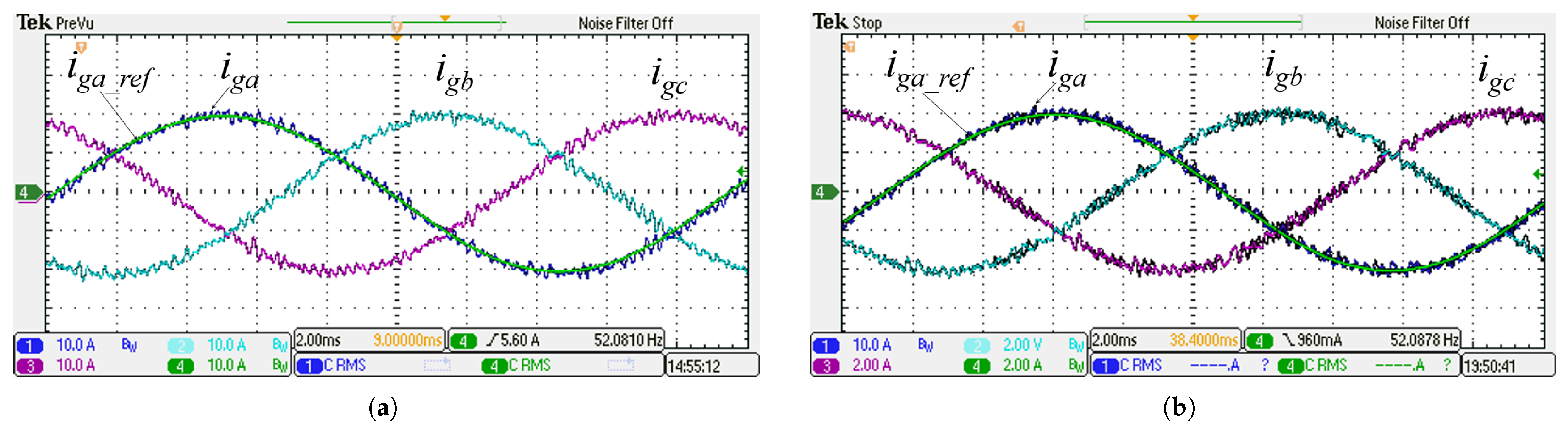
5.2. Current Tracking Transient Response
5.3. Influence of and N on Predictive Control Performance
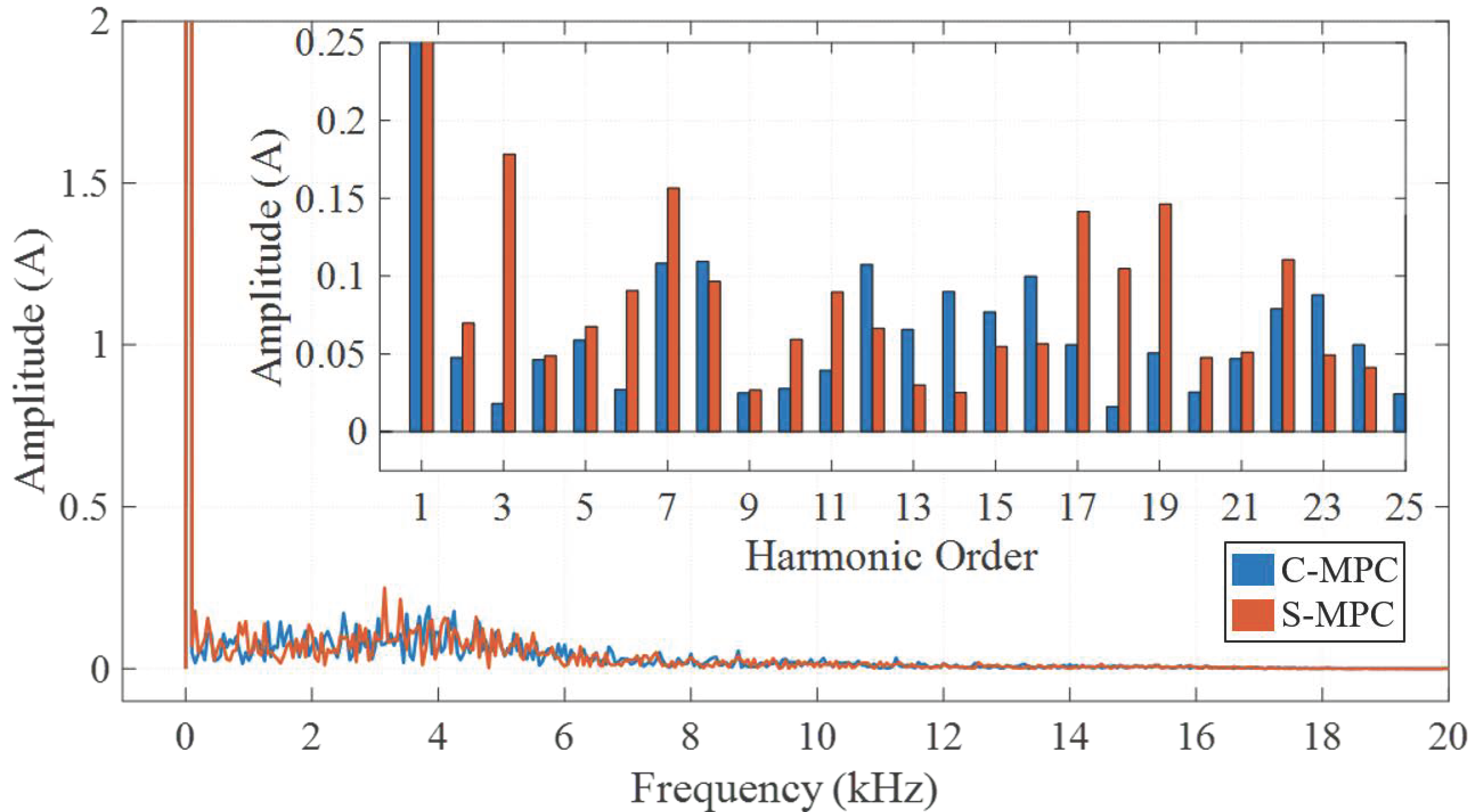
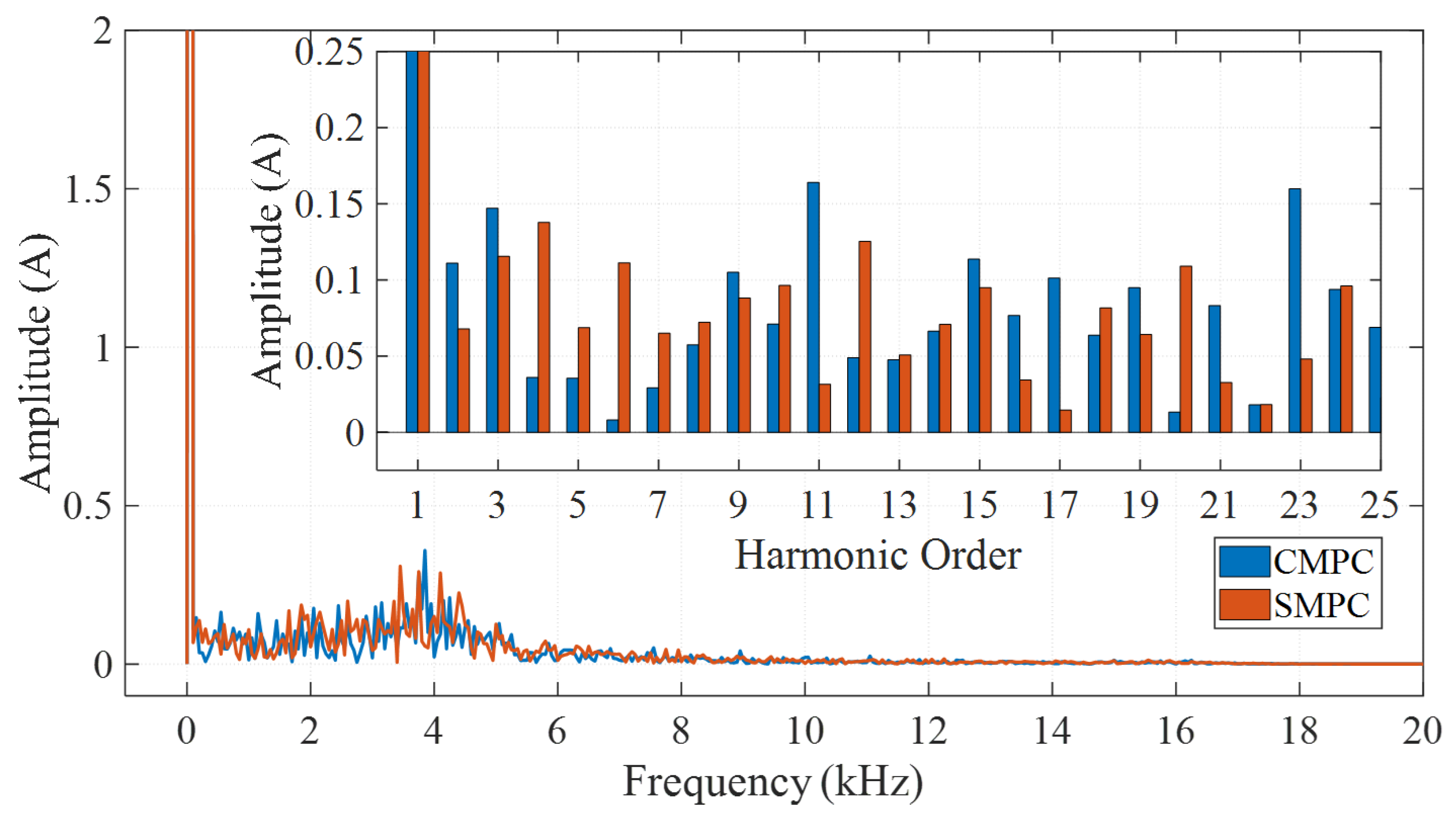
5.4. Voltage Harmonics
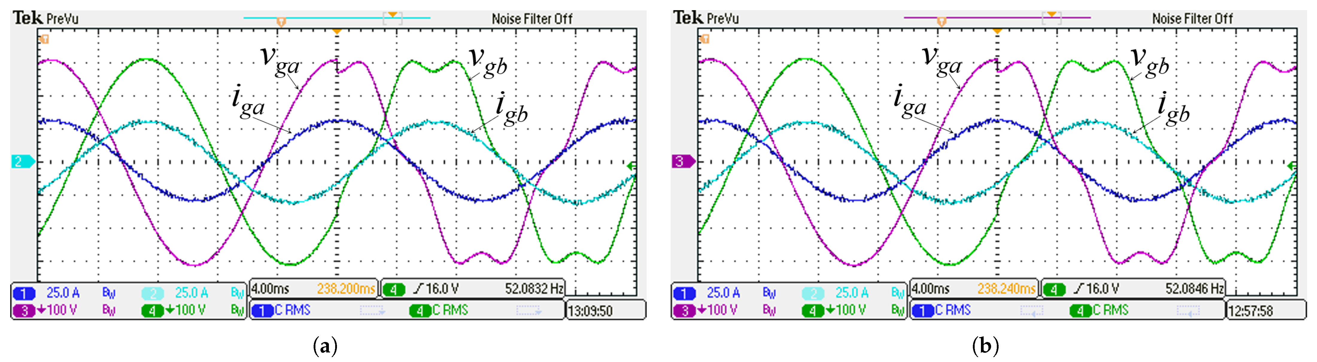
5.5. Voltage Sag and Swell
5.6. Sensitivity to Parameter Variations
5.7. Performance Summary
6. Conclusions
Author Contributions
Funding
Data Availability Statement
Conflicts of Interest
References
- Wang, G.; Li, X.; Zhang, H. Research on Microgrid Emission Reduction Mechanism and Emission Reduction Calculation Method. In Proceedings of the 2022 International Conference on Artificial Intelligence in Everything (AIE), Lefkosa, Cyprus, 2–4 August 2022; pp. 243–247. [Google Scholar] [CrossRef]
- Wang, Z.; Yang, B.; Wei, W.; Zhu, S.; Guan, X.; Sun, D. Multi-Energy Microgrids: Designing, Operation under New Business Models, and Engineering Practices in China. IEEE Electrif. Mag. 2021, 9, 75–82. [Google Scholar] [CrossRef]
- Liu, Q.; Caldognetto, T.; Buso, S. Review and Comparison of Grid-Tied Inverter Controllers in Microgrids. IEEE Trans. Power Electron. 2020, 35, 7624–7639. [Google Scholar] [CrossRef]
- Roselund, C.; Bernhardt, J. Lessons Learned Along Europe’s Road to Renewables. IEEE Spectrum. 2015. Available online: https://spectrum.ieee.org/lessons-learned-along-europes-road-to-renewables (accessed on 11 June 2025).
- IEEE Std 1547-2018; IEEE Standard for Interconnection and Interoperability of Distributed Energy Resources with Associated Electric Power Systems Interfaces. IEEE: Piscataway, NJ, USA, 2018.
- IEEE Std 519-2014; IEEE Recommended Practice and Requirements for Harmonic Control in Electric Power Systems. IEEE: Piscataway, NJ, USA, 2014. [CrossRef]
- IEC 61000-2-2:2002; Electromagnetic Compatibility (EMC)—Part 2-2: Environment–Compatibility Levels for Low-Frequency Conducted Disturbances and Signaling in Public Low-Voltage Power Supply Systems. IEC: Geneva, Switzerland, 2002.
- Kouro, S.; Malinowski, M.; Gopakumar, K.; Pou, J.; Franquelo, L.; Wu, B.; Rodriguez, J.; Perez, M.; Leon, J. Recent advances and industrial applications of multilevel converters. IEEE Trans. Ind. Electron. 2010, 57, 2553–2580. [Google Scholar] [CrossRef]
- Liu, J.; Shen, X.; Alcaide, A.M.; Yin, Y.; Leon, J.I.; Vazquez, S.; Wu, L.; Franquelo, L.G. Sliding Mode Control of Grid-Connected Neutral-Point-Clamped Converters via High-Gain Observer. IEEE Trans. Ind. Electron. 2022, 69, 4010–4021. [Google Scholar] [CrossRef]
- Yu, T.; Wan, W.; Duan, S. A Modulation Method to Eliminate Leakage Current and Balance Neutral-Point Voltage for Three-Level Inverters in Photovoltaic Systems. IEEE Trans. Ind. Electron. 2023, 70, 1635–1645. [Google Scholar] [CrossRef]
- Sanchez-Ruiz, A.; Mazuela, M.; Fernandez-Rebolleda, H.; Ceballos, S.; Perez-Basante, A.; Ibanez-Hidalgo, I.; Zubiaga, M.; Pou, J.; Beniwal, N.; Konstantinou, G. DC-Link Neutral Point Control for 3LNPC Converters Utilizing Selective Harmonic Elimination-PWM. IEEE Trans. Ind. Electron. 2022, 69, 8633–8644. [Google Scholar] [CrossRef]
- Wu, B. High-Power Converters and AC Drives, 1st ed.; Wiley-IEEE Press: Hoboken, NJ, USA, 2006. [Google Scholar]
- Vazquez, S.; Rodriguez, J.; Rivera, M.; Franquelo, L.G.; Norambuena, M. Model Predictive Control: A Review of Its Applications in Power Electronics. IEEE Ind. Electron. Mag. 2014, 8, 16–31. [Google Scholar] [CrossRef]
- Song, Y.; Liu, J.; Zhang, X. Research on Control Strategy of Three-level PV Grid-Connected Inverter Based on FCS-MPC. In Proceedings of the 2023 4th International Conference on Advanced Electrical and Energy Systems (AEES), Shanghai, China, 1–3 December 2023; pp. 39–44. [Google Scholar] [CrossRef]
- Karamanakos, P.; Liegmann, E.; Geyer, T.; Kennel, R. Model Predictive Control of Power Electronic Systems: Methods, Results, and Challenges. IEEE Open J. Ind. Appl. 2020, 1, 95–114. [Google Scholar] [CrossRef]
- Wang, X.; Hu, J.; Garcia, C.; Rodriguez, J.; Long, B. Robust Sequential Model-Free Predictive Control of a Three-Level T-Type Shunt Active Power Filter. IEEE Trans. Power Electron. 2024, 39, 9505–9517. [Google Scholar] [CrossRef]
- Vazquez, S.; Rodriguez, J.; Rivera, M.; Franquelo, L.G.; Norambuena, M. Model Predictive Control for Power Converters and Drives: Advances and Trends. IEEE Trans. Ind. Electron. 2017, 64, 935–947. [Google Scholar] [CrossRef]
- Novak, M.; Xie, H.; Dragicevic, T.; Wang, F.; Rodriguez, J.; Blaabjerg, F. Optimal Cost Function Parameter Design in Predictive Torque Control (PTC) Using Artificial Neural Networks (ANN). IEEE Trans. Ind. Electron. 2021, 68, 7309–7319. [Google Scholar] [CrossRef]
- Prajapati, D.; Dekka, A.; Ronanki, D.; Rodriguez, J. High-Performance Sequential Model Predictive Control of a Four-Level Inverter for Electric Transportation Applications. IEEE J. Emerg. Sel. Top. Ind. Electron. 2024, 5, 253–262. [Google Scholar] [CrossRef]
- Cortes, P.; Rivera, M.; Norambuena, M.; Rodriguez, J. Guidelines for weighting factors design in Model Predictive Control of power converters and drives. In Proceedings of the 2009 IEEE International Conference on Industrial Technology, Churchill, VIC, Australia, 10–13 February 2009; pp. 1–7. [Google Scholar] [CrossRef]
- Karamanakos, P.; Geyer, T. Guidelines for the Design of Finite Control Set Model Predictive Controllers. IEEE Trans. Power Electron. 2020, 35, 7434–7450. [Google Scholar] [CrossRef]
- Norambuena, M.; Rodriguez, J.; Zhang, Z.; Wang, F.; Garcia, C.; Kennel, R. A Very Simple Strategy for High-Quality Performance of AC Machines Using Model Predictive Control. IEEE Trans. Power Electron. 2019, 34, 794–800. [Google Scholar] [CrossRef]
- Zhang, H.; Tao, R.; Li, Z.; Zhang, X.; Ma, Z. Multivariable Sequential Model Predictive Control of LCL-Type Grid Connected Inverter. IET Power Electron. 2023, 16, 558–574. [Google Scholar] [CrossRef]
- Albalawi, H.; Zaid, S.A. Performance Improvement of a Grid-Tied Neutral-Point-Clamped 3-φ Transformerless Inverter Using Model Predictive Control. Processes 2019, 7, 856. [Google Scholar] [CrossRef]
- Herrera, F.; Mora, A.; Cárdenas, R.; Díaz, M.; Rodríguez, J.; Rivera, M. An Optimal Switching Sequence Model Predictive Control Scheme for the 3L-NPC Converter with Output LC Filter. Processes 2024, 12, 348. [Google Scholar] [CrossRef]
- Liu, X.; Zhang, Z.; Gao, F.; Norambuena, M.; Rodríguez, J.; Yavas, O.; Kennel, R. Sequential Direct Model Predictive Control for Grid-Tied Three-Level NPC Power Converters. In Proceedings of the 2018 IEEE International Power Electronics and Application Conference and Exposition (PEAC), Shenzhen, China, 4–7 November 2018; pp. 1–5. [Google Scholar] [CrossRef]
- Donoso, F.; Mora, A.; Cárdenas, R.; Angulo, A.; Sáez, D.; Rivera, M. Finite-Set Model-Predictive Control Strategies for a 3L-NPC Inverter Operating With Fixed Switching Frequency. IEEE Trans. Ind. Electron. 2018, 65, 3954–3965. [Google Scholar] [CrossRef]
- Baker, R.J. Power Electronics Handbook, 3rd ed.; Elsevier: Amsterdam, The Netherlands, 2011; pp. 247–248. [Google Scholar]
- Rodriguez, J.; Bernet, S.; Blaabjerg, F. Power Electronics for Renewable Energy Systems. IEEE Trans. Ind. Electron. 2008, 55, 2654–2671. [Google Scholar]
- Martins, D.C.; Júnior, R.M.A.; da Silva, J.L. Analysis of Capacitor Voltage Balancing Control in NPC Inverters. IEEE Trans. Power Electron. 2013, 28, 1911–1920. [Google Scholar]
- Wang, J.; Yang, Z.; He, X.; Zhang, H. A New Modulation Method for NPC Inverters with Capacitor Voltage Balancing. IEEE Trans. Ind. Electron. 2011, 58, 4135–4143. [Google Scholar]
- Wang, Y.; Xu, Y.; Xu, L. Voltage Balancing Control of Neutral-Point-Clamped Inverters with Unbalanced Loads. IEEE Trans. Power Electron. 2014, 29, 2254–2265. [Google Scholar]
- Blaabjerg, F.; Chen, Z. Power Electronics for Industrial Applications. IEEE Trans. Ind. Appl. 2006, 42, 937–945. [Google Scholar]
- Cortes, P.; Rivera, M.; Rodriguez, J. Neutral Point Voltage Balancing Control for NPC Inverters with Unequal Switching Frequencies. IEEE Trans. Power Electron. 2004, 19, 1164–1172. [Google Scholar]
- Doi, M.V.; Nguyen, B.X.; Nguyen, N.V. A Finite Set Model Predictive Current Control for Three-Level NPC Inverter with Reducing Switching State Combination. In Proceedings of the 2019 IEEE 4th International Future Energy Electronics Conference (IFEEC), Singapore, 25–28 November 2019; pp. 1–9. [Google Scholar]
- Rivera, M.; Pérez, M.; Baier, C.; Muñoz, J.; Yaramasu, V.; Wu, B.; Tarisciotti, L.; Zanchetta, P.; Wheeler, P. Predictive Current Control with Fixed Switching Frequency for an NPC Converter. In Proceedings of the 2015 IEEE 24th International Symposium on Industrial Electronics (ISIE), Buzios, Brazil, 3–5 June 2015; pp. 1034–1039. [Google Scholar]
- Vedreño-Santos, F.; Odavic, M.; Guan, Y.; Azar, Z.; Thomas, A.S.; Li, G.J.; Zhu, Z.Q. Design considerations for high-power converters interfacing 10 MW superconducting wind power generators. IET Power Electron. 2017, 10, 1389–1396. [Google Scholar] [CrossRef]
- Jin, J.; Zhang, Z.; Liu, Y. A Comprehensive Analysis of Inductor Current Ripple and Filter Design for Three-phase Three-Level Grid-Tie Inverter. In Proceedings of the 2024 IEEE 10th International Power Electronics and Motion Control Conference, Chengdu, China, 17–20 May 2024; pp. 4736–4742. [Google Scholar] [CrossRef]


| Switching State | Switch Signals | Output Voltage |
|---|---|---|
| −1 | (0, 0) | |
| 0 | (0, 1) | 0 |
| 1 | (1, 1) |
| State | |||||||||||
|---|---|---|---|---|---|---|---|---|---|---|---|
| 1 | 1 | 1 | 1 | 1 | 1 | 1 | 0 | 0 | |||
| 2 | 1 | 1 | 1 | 1 | 0 | 1 | 0 | ||||
| 3 | 1 | 1 | 1 | 1 | 0 | 0 | 0 | ||||
| 4 | 1 | 1 | 0 | 1 | 1 | 1 | 0 | 0 | |||
| 5 | 1 | 1 | 0 | 1 | 0 | 1 | 0 | 0 | |||
| 6 | 1 | 1 | 0 | 1 | 0 | 0 | 0 | ||||
| 7 | 1 | 1 | 0 | 0 | 1 | 1 | 0 | 0 | |||
| 8 | 1 | 1 | 0 | 0 | 0 | 1 | 0 | ||||
| 9 | 1 | 1 | 0 | 0 | 0 | 0 | |||||
| 10 | 0 | 1 | 1 | 1 | 1 | 1 | 0 | ||||
| 11 | 0 | 1 | 1 | 1 | 0 | 1 | 0 | 0 | 0 | ||
| 12 | 0 | 1 | 1 | 1 | 0 | 0 | 0 | 0 | |||
| 13 | 0 | 1 | 0 | 1 | 1 | 1 | 0 | 0 | |||
| 14 | 0 | 1 | 0 | 1 | 0 | 1 | 0 | 0 | 0 | 0 | 0 |
| 15 | 0 | 1 | 0 | 1 | 0 | 0 | 0 | 0 | |||
| 16 | 0 | 1 | 0 | 0 | 1 | 1 | 0 | ||||
| 17 | 0 | 1 | 0 | 0 | 0 | 1 | 0 | 0 | 0 | ||
| 18 | 0 | 1 | 0 | 0 | 0 | 0 | 0 | ||||
| 19 | 0 | 0 | 1 | 1 | 1 | 1 | 0 | ||||
| 20 | 0 | 0 | 1 | 1 | 0 | 1 | 0 | ||||
| 21 | 0 | 0 | 1 | 1 | 0 | 0 | 0 | 0 | |||
| 22 | 0 | 0 | 0 | 1 | 1 | 1 | 0 | ||||
| 23 | 0 | 0 | 0 | 1 | 0 | 1 | 0 | 0 | 0 | ||
| 24 | 0 | 0 | 0 | 1 | 0 | 0 | 0 | 0 | |||
| 25 | 0 | 0 | 0 | 0 | 1 | 1 | |||||
| 26 | 0 | 0 | 0 | 0 | 0 | 1 | 0 | ||||
| 27 | 0 | 0 | 0 | 0 | 0 | 0 | 0 | 0 |
| Description and Symbol | Value |
|---|---|
| Grid voltage (/) | 380 V/50 Hz |
| Dc–link voltage () | 800 V |
| Filter inductance per phase (L) | 5 mH |
| Resistance of filter inductor (R) | 0.8 |
| Dc–link capacitance ( and ) | 3.3 mF |
| C-MPC controller—Weighting Factor () | 0.4 |
| S-MPC controller—secondary evaluation (N) | 2 |
| Sampling Time () | 50 μs |
| SRF-PLL proportional gain () | 45 |
| SRF-PLL integral gain () | 970 |
| Voltage scaling factor () | 100 |
| Current scaling factor () | 10 |
| Test Case | Performance Index | C-MPC | S-MPC |
|---|---|---|---|
| Current reference step reference (20 to 30 A) (Figure 13) | 0.25 μs | 0.20 μs | |
| Time required to balance dc–link capacitor’s voltage (Figure 14) | 27 ms | 48 ms | |
| Current distortion during balancing (Figure 14) | 10.2% | 5.2% | |
| Steady-state current ripple (reference of 20 A) (Figure 10) | 2.0 A | 2.5 A | |
| Steady-state current distortion (reference of 20 A) (Figure 10) | 4.7% | 5.0% | |
| Steady-state current ripple (reference of 30 A) (Figure 18) | 3.0 A | 4.0 A | |
| Steady-state current distortion (reference of 30 A) (Figure 18) | 3.4% | 3.4% | |
| Current ripple for 0.5 L (reference of 30 A) (Figure 18) | 9.0 A | 9.0 A | |
| Current distortion for 0.5 L (reference of 30 A) (Figure 18) | 9.2% | 10.8% | |
| Current ripple for 2 L (reference of 30 A) (Figure 18) | 9.0 A | 1.0 A | |
| Current distortion for 2 L (reference of 30 A) (Figure 18) | 2.1% | 2.0% |
Disclaimer/Publisher’s Note: The statements, opinions and data contained in all publications are solely those of the individual author(s) and contributor(s) and not of MDPI and/or the editor(s). MDPI and/or the editor(s) disclaim responsibility for any injury to people or property resulting from any ideas, methods, instructions or products referred to in the content. |
© 2025 by the authors. Licensee MDPI, Basel, Switzerland. This article is an open access article distributed under the terms and conditions of the Creative Commons Attribution (CC BY) license (https://creativecommons.org/licenses/by/4.0/).
Share and Cite
Bonaldo, J.; Duan, B.; Rivera, M.; Ling, K.V.; Fantin, C.; Wheeler, P. Comprehensive Performance Assessment of Conventional and Sequential Predictive Control for Grid-Tied NPC Inverters: A Hardware-in-the-Loop Study. Energies 2025, 18, 3132. https://doi.org/10.3390/en18123132
Bonaldo J, Duan B, Rivera M, Ling KV, Fantin C, Wheeler P. Comprehensive Performance Assessment of Conventional and Sequential Predictive Control for Grid-Tied NPC Inverters: A Hardware-in-the-Loop Study. Energies. 2025; 18(12):3132. https://doi.org/10.3390/en18123132
Chicago/Turabian StyleBonaldo, Jakson, Beichen Duan, Marco Rivera, K. V. Ling, Camila Fantin, and Patrick Wheeler. 2025. "Comprehensive Performance Assessment of Conventional and Sequential Predictive Control for Grid-Tied NPC Inverters: A Hardware-in-the-Loop Study" Energies 18, no. 12: 3132. https://doi.org/10.3390/en18123132
APA StyleBonaldo, J., Duan, B., Rivera, M., Ling, K. V., Fantin, C., & Wheeler, P. (2025). Comprehensive Performance Assessment of Conventional and Sequential Predictive Control for Grid-Tied NPC Inverters: A Hardware-in-the-Loop Study. Energies, 18(12), 3132. https://doi.org/10.3390/en18123132