Impedance Characteristic-Based Frequency-Domain Parameter Identification Method for Photovoltaic Controllers

Abstract

With the large-scale integration of photovoltaic power plants—comprising power electronic devices—into power systems, electromagnetic transient simulation has become a key tool for ensuring power system security and stability. The accuracy of photovoltaic unit controller parameters is crucial for the reliability of such simulations. However, as the issue of sub/super-synchronous oscillations becomes increasingly prominent, existing parameter identification methods are primarily based on high/low voltage ride-through characteristics. This limits the applicability of the identification results to specific scenarios and lacks targeted simulation and parameter identification research for sub/super-synchronous oscillations. To address this gap, this study proposes a mathematical model tailored for sub/super-synchronous oscillations and performs sensitivity analysis of converter control parameters to identify dominant parameters across different frequency bands. A frequency-segmented parameter identification method is introduced, capable of fast convergence without relying on a specific optimization algorithm. Finally, the proposed method’s identification results are compared with actual values, voltage ride-through-based identification, particle swarm optimization results, and results under uncertain conditions. It was found that, compared with traditional identification methods, the proposed method reduced the maximum identification error from 7.67% to 4.3% and the identification time from 2 h to 1 h. The maximum identification error of other intelligent algorithms was 5%, with a difference of less than 1% compared to the proposed method. The identified parameters were applied under conditions of strong irradiation (1000 W/m²), weak irradiation (300 W/m²), rapidly varying oscillation frequency, and constant oscillation frequency, and the output characteristics were all close to those of the original parameters. The effectiveness and superiority of the proposed method have been validated, along with its broad applicability to different intelligent algorithms and its robustness under uncertain conditions such as environmental variations and grid frequency fluctuations.

1. Introduction

With the continuous development of new energy power generation in China [1,2], photovoltaic power has been widely applied in power systems due to its excellent economic efficiency, reliability, and sustainability [3,4]. While photovoltaic energy improves the energy structure in China, it also affects the stability of power systems [5,6]. As large-scale photovoltaic power plants are integrated into power systems [7,8], several cases of sub-synchronous and super-synchronous oscillations have occurred in new energy systems [9,10]. For example, sub-synchronous and super-synchronous oscillations caused by the interaction between new energy sources and transmission lines were reported in Texas, USA, in 2009, and in Hebei, China, in 2012 [11,12]. In 2015, similar oscillations occurred in Hami, Xinjiang, China, when new energy sources were integrated into a weak power grid, resulting in the trip of nearby thermal power units [13]. These incidents have made the study of sub-synchronous and super-synchronous oscillation response characteristics of photovoltaic systems increasingly important [14].

Currently, the primary methods for studying photovoltaic power generation systems can be categorized into the eigenvalue analysis method, time-domain simulation method, and impedance-based analysis method [15]. The eigenvalue analysis method evaluates system stability by solving the state-space equations of the small-signal model and observing the location of eigenvalues in the complex plane, thus analyzing the oscillation characteristics of the system. However, this method involves a large computational burden and complex calculation processes. The time-domain simulation method analyzes the oscillation characteristics of the system by observing the time-varying trends of system variables during the simulation process, but it heavily relies on the accuracy of the established model. The impedance-based analysis method, on the other hand, constructs an impedance model and conducts frequency sweeping to obtain the impedance characteristics of the system across the full frequency range. By combining the obtained impedance characteristics with appropriate stability criteria, the oscillation characteristics of the system under different frequency ranges can be analyzed. This method has gradually become the primary approach for studying sub-synchronous and super-synchronous oscillation characteristics.

According to current research on the transient stability of photovoltaic power systems [16], this study on the sub-synchronous and super-synchronous oscillation phenomena in photovoltaic power generation systems mainly focuses on the simulation and analysis of the model. Since the converter control parameters are unknown in the simulation model, errors will lead to inaccurate analysis of the sub-synchronous and super-synchronous oscillation phenomena. Therefore, researching the impact of converter control parameters on the oscillatory characteristics of photovoltaic power generation systems is of significant importance. However, due to reasons such as commercial confidentiality, manufacturers typically only provide “black-box” models, with unknown internal structures and control parameters of the converter, lacking an understanding of the relationship between the controller and the grid in terms of sub-synchronous and super-synchronous oscillations. This severely hampers research into the oscillatory characteristics of photovoltaic power generation systems. Given these two factors, research on the identification of photovoltaic converter control parameters is of great significance.

Existing parameter identification methods are primarily based on the dynamic response characteristics under high/low voltage ride-through conditions. For example, the literature [17] proposed a dq-axis decoupling parameter identification strategy for the dual-loop control model of inverters based on the damping least squares method. However, this approach shows high identification accuracy for the outer voltage loop but relatively low accuracy for the inner current loop. The literature [18] introduced a stepwise identification method based on the random forest algorithm, which filters high-correlation observables. Nevertheless, this method only verified the accuracy of the identification results under LVRT (low voltage ride through) conditions ranging from 20% to 80%. The literature [19] proposed a distributed identification method based on an improved grey wolf optimization algorithm, which avoids the cascade issue between the inner and outer PI controllers by selecting three observable variables from both loops. However, it fails to ensure consistent identification accuracy for both the inner and outer loop control parameters. The literature [20] employed a parameter identification method based on a genetic algorithm to identify the control parameters of the rotor-side converter in a doubly fed induction generator in the time domain. Nevertheless, the identified parameters still exhibited certain deviations from the original parameters under steady-state conditions, requiring further analysis. The literature [21] applied the profile likelihood method to identify inverter control parameters by observing the impact of parameter variations on the external characteristics of the generating unit. However, this method encounters difficulty in achieving accurate identification results under minor fault conditions. The aforementioned studies have only validated the accuracy of the proposed parameter identification methods under specific High/Low Voltage Ride-Through scenarios but have not ensured that the output characteristics of the simulation model match the actual values under sub-synchronous and super-synchronous oscillation conditions. To more intuitively highlight the advantages and disadvantages of each identification method, the methods mentioned above have been organized into a table format as shown in

Table 1. Research status of identification methods.

Reference Title	Proposed Method	Problem Addressed	Limitations
Reference [16]	Parameter Identification of Converter Dual-Loop Control Model with DQ-Axis Decoupling Based on Damped Least Squares	The time scale of the model does not match the time scale of the transient characteristic analysis, leading to discrepancies in parameters during multiple disturbance identifications, resulting in poor consistency of the identification results	The voltage outer loop parameter identification accuracy is high, while the current inner loop parameter identification accuracy is low
Reference [17]	Stepwise Identification Method Based on Random Forest Algorithm for Selecting Highly Correlated Observables	The issue of low parameter identification accuracy for the existing doubly fed wind turbine GSC LVRT and the neglect of high-sensitivity parameters during the identification process	The accuracy of the identification results has not been verified outside the 20–80% low voltage ride-through conditions
Reference [18]	Distributed Identification Method Based on Improved Grey Wolf Optimization Algorithm	The mutual interference caused by the cascading between the inner and outer loop PI controllers leads to inaccurate identification	It is not possible to guarantee the consistency of the identification accuracy of the inner and outer loop control parameters.
Reference [19]	Parameter Identification Method Based on Genetic Algorithm	During the identification process of the integral part, input and output data are typically transformed to the complex frequency domain, and the system is discretized. The use of genetic algorithm for identification leads to a significant computational burden, which in turn prolongs the identification time	In steady-state conditions, there is a certain error between the identification results and the original parameters, which requires further analysis
Reference [20]	Profile Likelihood Method	During the simulation process, the controller parameters of the large wind farm are unknown, and only the external characteristics and performance indicators of the wind turbines are provided, which makes the simulation study challenging	Parameter identification is more difficult under minor fault conditions

.

To address the aforementioned issues, the research objectives of this paper are as follows:

(1)

Propose a mathematical model suitable for subsynchronous oscillations;

(2)

Analyze the sensitivity of the converter control parameters and identify the dominant parameters in different frequency bands;

(3)

A frequency-based parameter identification method is proposed based on the relationship between different frequency bands and dominant parameters. The effectiveness of the proposed method is then verified through a white-box model and controller from the manufacturer.

On this basis, this paper proposes a parameter identification method based on impedance characteristics. Firstly, an electromagnetic transient model of the photovoltaic power generation unit is established. Secondly, a sensitivity analysis of each parameter is conducted, followed by the design of a frequency-segmented control parameter identification process. By validating the accuracy of the identified parameters under sub-synchronous and super-synchronous oscillation scenarios, this method effectively avoids the limitations of existing methods that rely solely on high/low voltage ride-through conditions.

2. Electromagnetic Transient Model of Photovoltaic Power Generation Unit

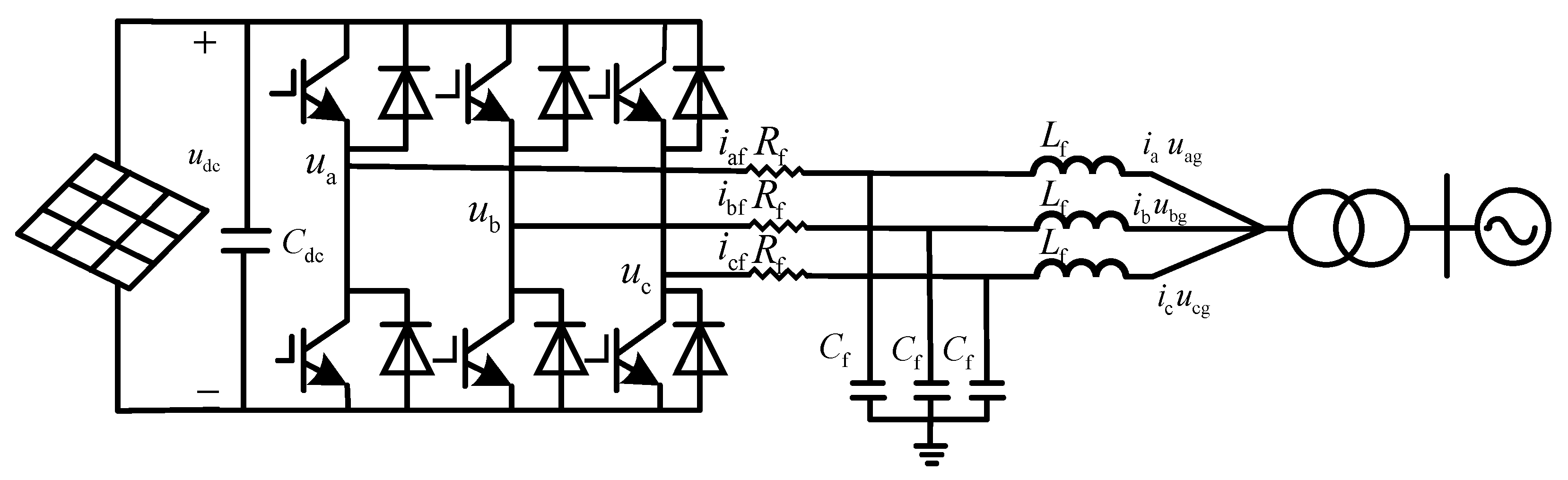
2.1. Main Circuit Topology

The photovoltaic power generation unit model primarily consists of a photovoltaic array, inverter, filter, step-up transformer, and other components. The mainstream converter topologies currently include unipolar and bipolar structures, and inverters can also be categorized into various forms such as two-level and three-level configurations. However, since this study focuses on the oscillation issues between converter control and the power grid, a unified assumption of a unipolar two-level converter topology is adopted to avoid interference with the system stability analysis. Furthermore, the equivalent average model of this topology is used, and switching details are neglected, so as to more clearly focus on the analysis of system stability characteristics. The topology structure of the photovoltaic power generation unit [22,23] is shown in Figure 1.

In the figure: u_dc represents the output voltage of the photovoltaic array; u_ag, u_bg, u_cg denote the three-phase voltage at the point of common coupling; u_a, u_b, u_c represent the three-phase output voltage of the inverter; i_af, i_bf, i_cf denote the output current of the inverter; C_dc represents the DC (direct current)-link capacitor; R_f, L_f, C_f denote the parameters of the grid-side RLC filter (resistor-inductor-capacitor filter).

2.2. Grid-Connected Inverter Modeling

As shown in Figure 1, the inverter converts the DC voltage output from the photovoltaic array into an AC (alternating current) voltage, which is then fed into the grid. Based on the circuit structure, the state-space equations of the inverter can be derived, as expressed in Equations (1) and (2). These equations serve as the basis for studying the input-output characteristics of the inverter.

$$\left\{\begin{array}{c}{u}_{\mathrm{a}}=L_{\mathrm{f}}{\displaystyle \frac{\mathrm{d}{i}_{\mathrm{af}}}{\mathrm{d}t}}+R_{\mathrm{f}}{i}_{\mathrm{af}}+u_{\mathrm{ag}}\\ u_{\mathrm{b}}=L_{\mathrm{f}}{\displaystyle \frac{\mathrm{d}{i}_{\mathrm{bf}}}{\mathrm{d}t}}+R_{\mathrm{f}}{i}_{\mathrm{bf}}+u_{\mathrm{bg}}\\ u_{\mathrm{c}}=L_{\mathrm{f}}{\displaystyle \frac{\mathrm{d}{i}_{\mathrm{cf}}}{\mathrm{d}t}}+R_{\mathrm{f}}{i}_{\mathrm{cf}}+u_{\mathrm{cg}}\end{array}\right.\mathrm{k}$$

(1)

$$\left\{\begin{array}{c}{i}_{\mathrm{af}}=i_{\mathrm{a}}+C_{\mathrm{f}}{\displaystyle \frac{\mathrm{d}(u_{\mathrm{ag}}-u_{\mathrm{bg}})}{\mathrm{d}t}}+C_{\mathrm{f}}{\displaystyle \frac{\mathrm{d}(u_{\mathrm{ag}}-u_{\mathrm{cg}})}{\mathrm{d}t}}\\ i_{\mathrm{bf}}=i_{\mathrm{b}}+C_{\mathrm{f}}{\displaystyle \frac{\mathrm{d}(u_{\mathrm{bg}}-u_{\mathrm{ag}})}{\mathrm{d}t}}+C_{\mathrm{f}}{\displaystyle \frac{\mathrm{d}(u_{\mathrm{bg}}-u_{\mathrm{cg}})}{\mathrm{d}t}}\\ i_{\mathrm{cf}}=i_{\mathrm{c}}+C_{\mathrm{f}}{\displaystyle \frac{\mathrm{d}(u_{\mathrm{cg}}-u_{\mathrm{ag}})}{\mathrm{d}t}}+C_{\mathrm{f}}{\displaystyle \frac{\mathrm{d}(u_{\mathrm{cg}}-u_{\mathrm{bg}})}{\mathrm{d}t}}\end{array}\right.$$

(2)

By applying a coordinate transformation, the above equations are converted into the synchronous rotating reference frame. Considering that the influence of the filter capacitor C_f is relatively small [22], the capacitor can be neglected, resulting in the mathematical model as expressed in Equation (3).

$$\left\{\begin{array}{c}{L}_{\mathrm{f}}{\displaystyle \frac{\mathrm{d}{i}_{\mathrm{d}}}{\mathrm{d}t}}=u_{\mathrm{d}}-\omega L_{\mathrm{f}}{i}_{\mathrm{q}}-i_{\mathrm{df}}{R}_{\mathrm{f}}-u_{\mathrm{dg}}\\ L_{\mathrm{f}}{\displaystyle \frac{\mathrm{d}{i}_{\mathrm{q}}}{\mathrm{d}t}}=u_{\mathrm{q}}+\omega L_{\mathrm{f}}{i}_{\mathrm{d}}-i_{\mathrm{qf}}{R}_{\mathrm{f}}-u_{\mathrm{qg}}\end{array}\right.$$

(3)

In the equation: i_df, i_qf represent the current components of the inverter output current after being transformed into the synchronous rotating reference frame; u_dg, u_qg denote the voltage components of the three-phase voltage at the point of common coupling after being transformed into the synchronous rotating reference frame; u_d, u_q represent the voltage components of the inverter output voltage after being transformed into the synchronous rotating reference frame.

All voltage and current variables in Equations (1)–(3), including i_a, i_b, i_c, i_af, i_bf, i_cf, i_df, i_qf, u_a, u_b, u_c, u_ag, u_bg, u_cg, u_dg, u_qg, u_d, and u_q, are intermittent and a function of time.

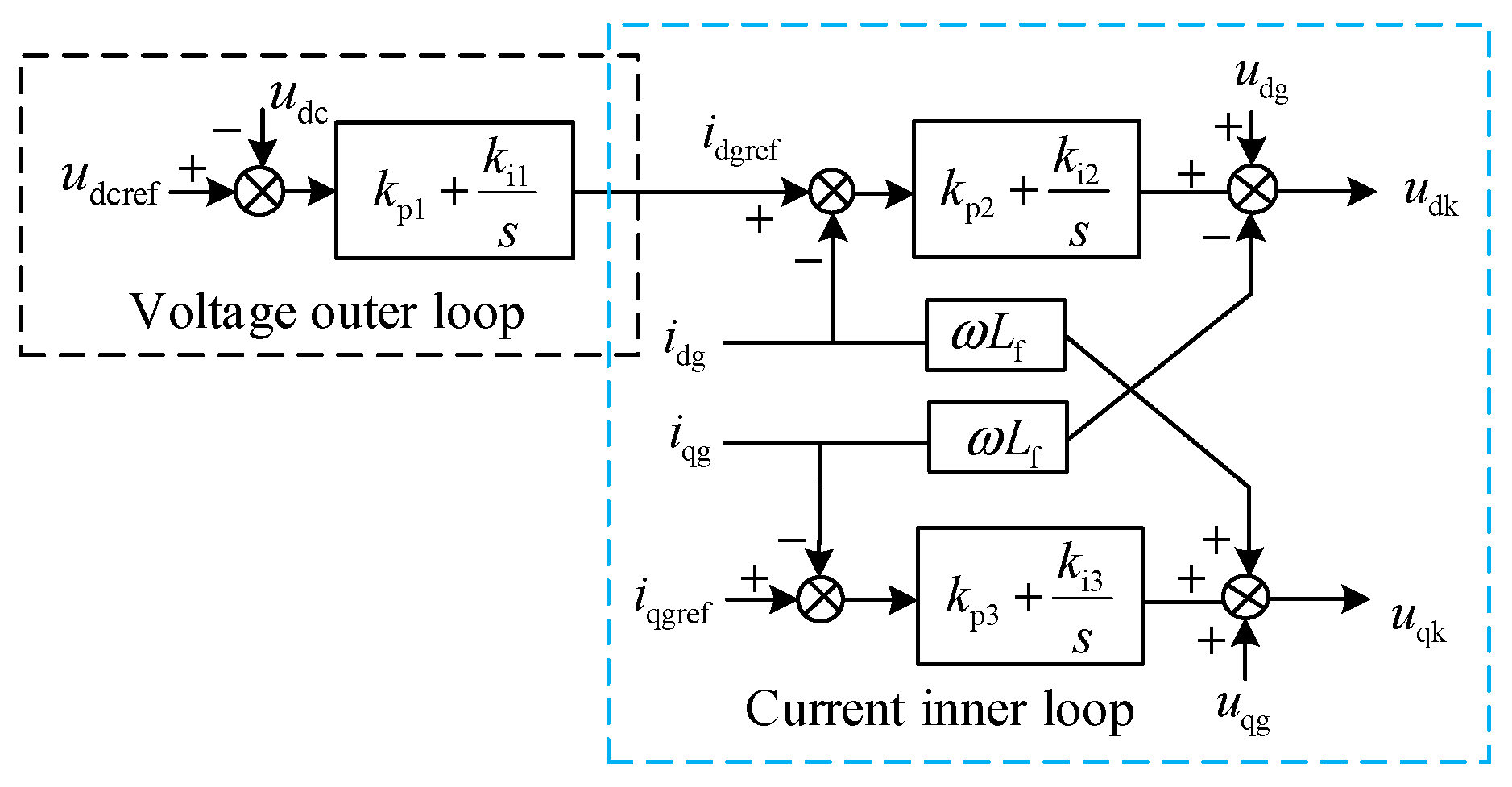
2.3. Controller Modeling

The inverter control in the photovoltaic power generation unit adopts a typical dual-loop control strategy, which consists of an outer voltage control loop and an inner current control loop. On the d-axis, the outer loop employs a PI (proportional-integral) controller to compare the DC-link voltage with its reference value, and the resulting voltage deviation is converted into an active current reference. The inner loop then regulates the active power output of the inverter by tracking the active current reference and generating the inverter’s reference voltage through PI control. On the q-axis, the inner loop directly controls the reactive current. The PI controller processes the reactive current reference, which is typically set to zero, to generate the corresponding reference voltage for the inverter. The control block diagram is shown in Figure 2.

In the figure: u_dcref denotes the DC voltage reference; i_dgref represents the active current reference; i_qgref represents the reactive current reference. Based on the aforementioned dual-loop control structure consisting of an outer voltage control loop and an inner current control loop, the state-space equations of the inverter can be derived as shown in Equation (4).

$$\left\{\begin{array}{c}{\displaystyle \frac{\mathrm{d}{x}_1}{\mathrm{d}t}}=u_{\mathrm{dcref}}-u_{\mathrm{dc}}\\ {\displaystyle \frac{\mathrm{d}{x}_2}{\mathrm{d}t}}=i_{\mathrm{dgref}}-i_{\mathrm{dg}}\\ {\displaystyle \frac{\mathrm{d}{x}_3}{\mathrm{d}t}}=i_{\mathrm{qgref}}-i_{\mathrm{qg}}\\ i_{\mathrm{dgref}}=k_{\mathrm{p}1}(u_{\mathrm{dcref}}-u_{\mathrm{dc}})+k_{\mathrm{il}}{x}_1\\ u_{\mathrm{dk}}=k_{\mathrm{p}2}(i_{\mathrm{dgref}}-i_{\mathrm{dg}})+k_{\mathrm{i}2}{x}_2+u_{\mathrm{dg}}-\omega L_{\mathrm{f}}{i}_{\mathrm{qg}}\\ u_{\mathrm{qk}}=k_{\mathrm{p}3}(i_{\mathrm{qgref}}-i_{\mathrm{qg}})+k_{\mathrm{i}3}{x}_3+u_{\mathrm{qg}}+\omega L_{\mathrm{f}}{i}_{\mathrm{dg}}\end{array}\right.$$

(4)

In the equation: k_pj, k_ij represent the control parameters of the inverter for the outer voltage loop and inner current loop, respectively; u_dk, u_qk denote the control signals of the inverter.

3. Frequency-Division Parameter Identification Principle

3.1. Controller Parameter Sensitivity Analysis

3.1.1. Sensitivity Analysis Methodology

Among the various control parameters of the converter, different control parameters dominate the impedance response characteristics in different frequency bands. Identifying the parameters using the full-frequency impedance characteristics not only results in a slow identification process but also reduces the accuracy of parameter identification. Among these parameters, high-sensitivity control parameters have a stronger influence on the system’s output characteristics, while low-sensitivity control parameters have a weaker influence. Therefore, prior to parameter identification, sensitivity analysis of the parameters to be identified should be conducted. By identifying the dominant parameters in different frequency bands, the accuracy and speed of parameter identification can be significantly improved.

In this paper, the time-domain simulation method is adopted for impedance scanning. By injecting small disturbance signals across the full frequency band, system oscillations are induced. Subsequently, appropriate observation variables are selected to analyze the sensitivity of the parameters to be identified in different frequency bands. The specific testing steps are as follows:

(1)

Simulation Platform

Based on the proposed model, a photovoltaic power generation unit simulation model is built on the SIMULINK platform, with specific parameters shown in

Table 2. Specific parameter settings of the model.

Parameter Name	Parameter Value
Power output of the generation unit/kW	255
DC-side voltage/kV	1.5
AC-side voltage/kV	0.8
Grid-side voltage/kV	37
Equivalent series resistance of the step-up transformer/Ω	0.00431746
Leakage inductance of the step-up transformer/H	0.03475
Filter inductance/H	0.0003, 0.003
Filter capacitance/F	5.5953 × 10−5
DC resistance/Ω	5000
DC capacitance/F	0.2

.

(2)

Multi-Parameter Stepwise Testing

Based on the original values of the parameters to be identified, adjust the control parameter values by a certain percentage each time, and then inject the modified control parameter values into the simulation model.

(3)

Time-Domain Response Analysis

The system synchronization frequency is 50 Hz. A small perturbation signal ranging from 1 Hz to 1000 Hz is injected at the low-voltage side of the step-up transformer in the photovoltaic power generation unit, thereby inducing sub/super-synchronous oscillations in the system. The system output characteristics under oscillations at each frequency are recorded.

(4)

Results Analysis

Perform a Fast Fourier Transform on the voltage and current signals to convert them into the frequency domain. This transformation enables a spectral representation that visually illustrates the intensity and characteristics of sub-/super-synchronous oscillations, thereby further validating the model’s accuracy. Additionally, the impedance characteristics of the photovoltaic generation unit at different frequencies are calculated and used as observables. By analyzing these impedance characteristics alongside the system’s original parameter model, the influence of various converter control parameters on system performance across different frequency bands is determined. High-sensitivity parameters are then identified for final parameter estimation. The sensitivity calculation formula is given by Equation (5).

$$S_{\theta i}={\displaystyle \frac{\frac{y({\theta }_1,\dots \hspace{0.17em},{\theta }_i+\Delta {\theta }_i,\dots \hspace{0.17em},{\theta }_m,f_j)-y({\theta }_1,\dots \hspace{0.17em},{\theta }_i,\dots \hspace{0.17em},{\theta }_m,f_k)}{y({\theta }_1,\dots \hspace{0.17em},{\theta }_i,\dots \hspace{0.17em},{\theta }_m,f_k)}}{\frac{\Delta {\theta }_i}{{\theta }_i}}}$$

(5)

where S_θi represents the trajectory sensitivity of the control parameter θ_i, Δθ_i is the deviation of the control parameter, θ_i is the original value of the control parameter, and y is the observable quantity, which in this case is the admittance of the photovoltaic power generation system. f_k represents the current injected disturbance frequency. The oscillation interval is divided into low-frequency (1–10 Hz), medium-frequency (10–100 Hz), and high-frequency (100–1000 Hz) ranges. It can be observed that each frequency range contains multiple impedance characteristics, and for ease of analysis, the average and maximum sensitivity values within each range are taken for analysis.

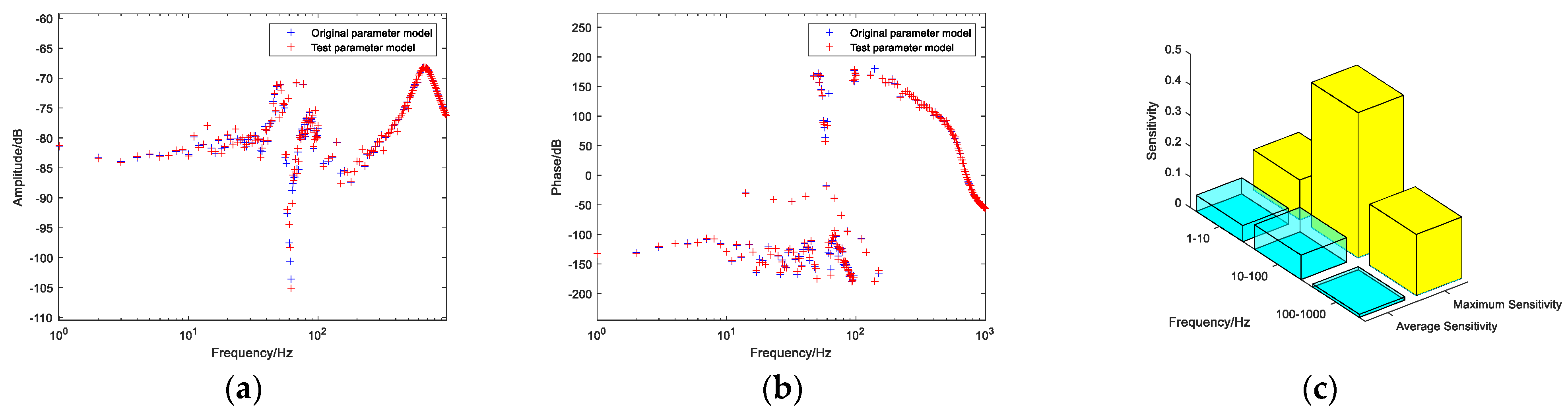
3.1.2. Sensitivity Analysis Results

The control parameters to be identified include the voltage outer loop control parameters k_{p_v}, k_{i_v} and the current inner loop control parameters k_{p_idg}, k_{i_idg}, k_{p_iqg}, k_{i_iqg}. The original values of these parameters are shown in

Table 3. Original values of control parameters.

Parameter	kp_v	ki_v	kp_idg	ki_idg	kp_iqg	ki_iqg
Original value	−60	−9000	3	3	3	3

.

The test parameters are set to twice the original parameter values. After starting the test, all parameters other than the test parameters are kept unchanged, and the new control parameter samples are injected into the simulation model. The impedance characteristics are calculated, and the error between the injected impedance characteristics of the original parameters and the new ones is determined. The specific test results are as follows:

(1)

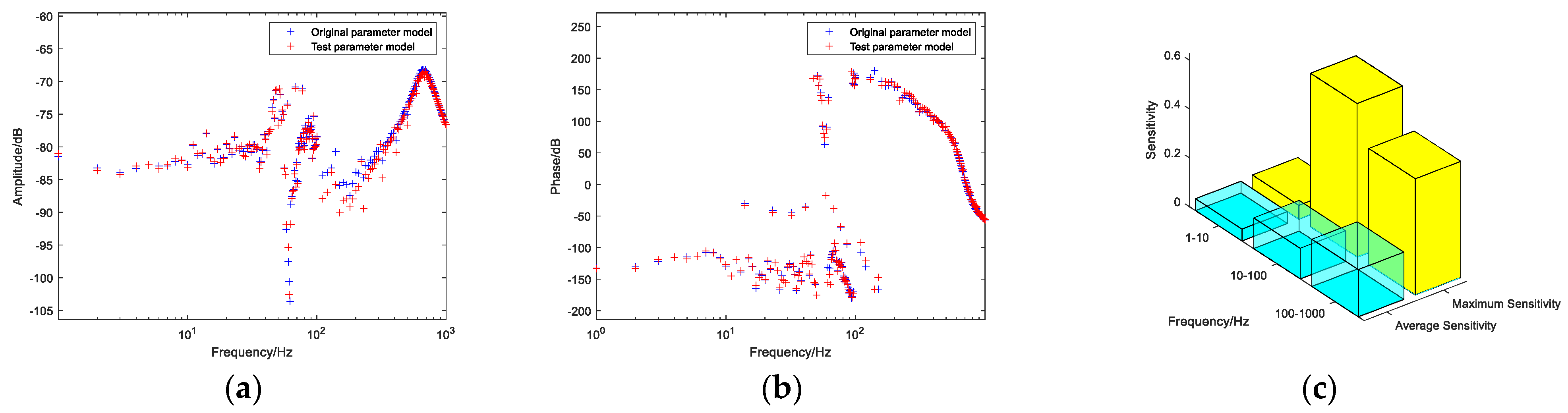
The sensitivity test for the control parameter k_{p_v} was conducted, and the test results are shown in Figure 3.

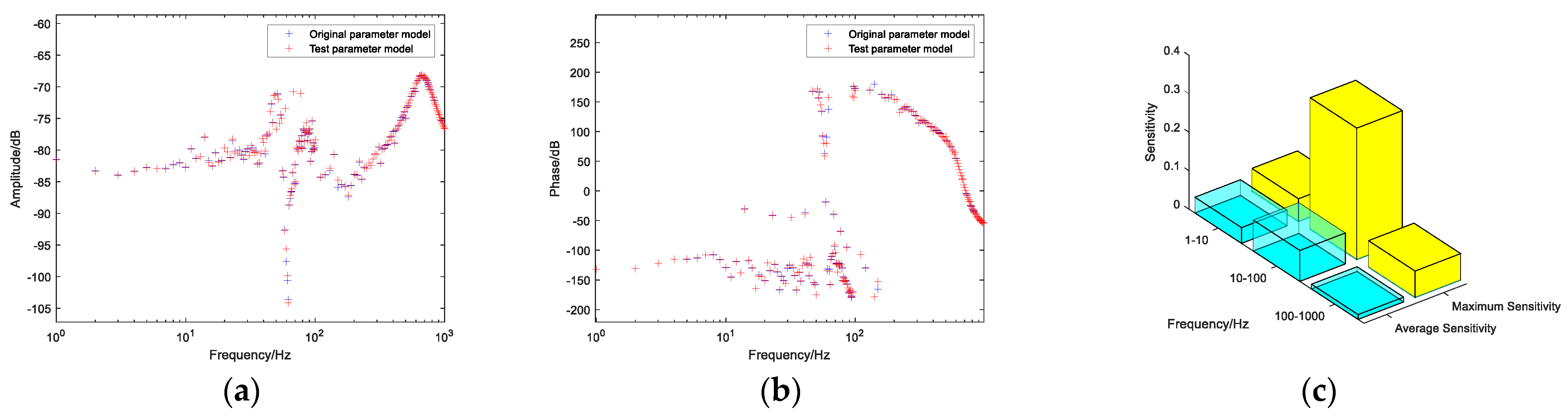
By observing the impedance characteristics in Figure 3, it can be seen that changing the voltage outer-loop control parameter k_{p_v} has no effect on the impedance phase-frequency characteristics of the test parameter model. The amplitude-frequency characteristics in the low-frequency range are almost identical to those of the original parameter, while significant differences appear in the mid- and high-frequency ranges. Observing the sensitivity graph, it is found that the average sensitivity of this parameter is low in the low-frequency band but shows higher average sensitivity in the mid- and high-frequency bands, with certain operating points exhibiting extremely high sensitivity, making it more identifiable.

(2)

The sensitivity test for the control parameter k_{i_v} was conducted, and the test results are shown in Figure 4.

By observing the impedance characteristics in Figure 4, it can be seen that changing the voltage outer-loop control parameter k_{i_v} has no effect on the impedance phase-frequency characteristics of the test parameter model. The amplitude-frequency characteristics in the low-frequency and high-frequency ranges are almost identical to those of the original parameter model, while there is some difference in the mid-frequency range. Observing the sensitivity graph, it is found that the average sensitivity of this parameter is lower in the high-frequency band, while the average sensitivity is relatively higher in the low and mid-frequency bands, with certain operating points showing large sensitivity, making it more identifiable.

(3)

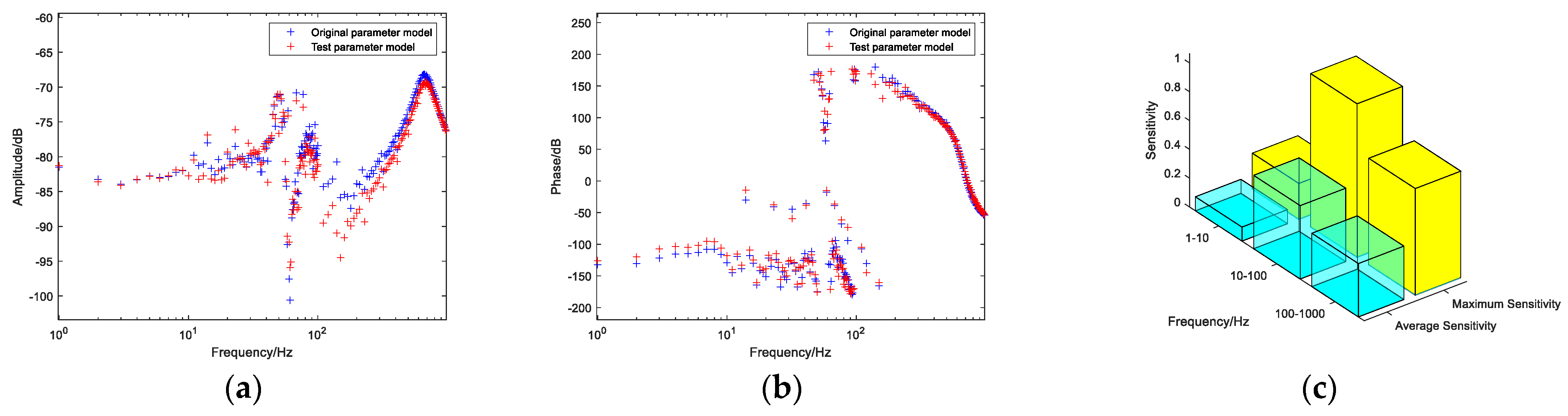
The sensitivity test for the control parameter k_{p_idg} was conducted, and the test results are shown in Figure 5.

By observing the impedance characteristics in Figure 5, it can be seen that changing the current inner-loop control parameter k_{p_idg} results in certain differences in the impedance phase-frequency characteristics between the test parameter model and the original parameter model in the low- and mid-frequency ranges, while they remain almost identical in the high-frequency range. The amplitude-frequency characteristics are nearly the same as the original parameter model in the low-frequency range but show significant differences in the mid- and high-frequency ranges. Observing the sensitivity graph, it is found that this parameter exhibits higher average sensitivity in the mid- and high-frequency bands, indicating strong identifiability.

(4)

The sensitivity test for the control parameter k_{i_idg} was conducted, and the test results are shown in Figure 6.

By observing the impedance characteristics in Figure 6, it can be seen that changing the current inner-loop control parameter k_{i_idg} has no effect on the impedance phase-frequency characteristics of the test parameter model. The amplitude-frequency characteristics remain nearly identical to the original parameter model in the low- and high-frequency ranges but exhibit significant differences in the mid-frequency range. Observing the sensitivity graph, it is found that this parameter has relatively high average sensitivity in the low- and mid-frequency bands, indicating strong identifiability.

(5)

The sensitivity test for the control parameter k_{p_iqg} was conducted, and the test results are shown in Figure 7.

By observing the impedance characteristics in Figure 7, it can be seen that changing the current inner-loop control parameter k_{p_iqg} results in a significant error between the impedance phase-frequency and amplitude-frequency characteristics of the test parameter model and the original model in the low-frequency range. In the mid- and high-frequency ranges, the characteristics remain largely consistent with the original parameter model. However, the amplitude-frequency characteristics exhibit significant differences from the original model across the entire frequency range. Observing the sensitivity graph, it is found that this parameter has high average sensitivity in the low-, mid-, and high-frequency bands, indicating strong identifiability.

(6)

The sensitivity test for the control parameter k_{i_iqg} was conducted, and the test results are shown in Figure 8.

By observing the impedance characteristics in Figure 8, it can be seen that changing the current inner-loop control parameter k_{i_iqg} results in impedance phase-frequency and amplitude-frequency characteristics that remain largely consistent with the original parameter model across the entire frequency range. Observing the sensitivity graph, it is found that there are individual operating points in the mid-frequency range with relatively high sensitivity. Compared to the high-frequency range, the low- and mid-frequency ranges exhibit higher average sensitivity, indicating a certain degree of identifiability.

Based on the sensitivity test results of each parameter, considering the influence of individual points with extremely high sensitivity, the average sensitivity is used as the primary evaluation criterion, as it provides a clearer representation of the sensitivity level of control parameters. Additionally, given that the dq-axis (direct axis and quadrature axis) current inner loops share the same mathematical model with identical original control parameters and exhibit similar sensitivity characteristics, a unified set of PI control parameters is selected for both axes.

3.2. Mechanism of Frequency-Division Parameter Identification

According to the sensitivity test results of the converter control parameters, the proportional control parameters k_{p_v} and k_{p_idg} exhibit higher sensitivity in the high-frequency range. This is because, at high frequencies, the disturbance frequency is larger, resulting in a minimal effect of the integral control component in the controller. Consequently, any change in the proportional control parameters significantly impacts the control characteristics of the converter, thereby affecting the impedance characteristics of the system.

Similarly, the integral control parameters k_{i_v} and k_{i_idg} exhibit higher sensitivity in the low- and mid-frequency ranges. This is because, at low frequencies, the disturbance frequency is relatively small, leading to a greater effect of the integral control component in the controller. As a result, any change in the integral control parameters significantly influences the control characteristics of the converter, thereby affecting the impedance characteristics of the system.

4. Impedance-Based Frequency-Division Parameter Identification Method for Photovoltaic Power Generation Unit Controllers

4.1. Parameter Identification Steps

This paper proposes a frequency-division parameter identification method based on impedance characteristics, selecting the impedance characteristics of the photovoltaic generation unit as the observation metric for identification. The entire parameter identification process is divided into the following steps:

(1)

Target Parameter Definition: Under the sub-synchronous and super-synchronous oscillation scenarios, multiple sets of controller parameters can be identified, such as voltage outer loop control parameters and current inner loop control parameters. Based on the content of this paper, the PI control parameters of the converter’s voltage outer loop and current inner loop are identified.

(2)

Sensitivity Analysis of Parameters to be Identified: Different manufacturers’ converter control parameters vary significantly. Low-sensitivity control parameters have a weaker impact on output characteristics, and changing their values does not significantly alter the output characteristic curve. Performing parameter identification on these parameters results in low iteration efficiency and unclear effects, making it difficult to determine typical values. Based on the sensitivity test results from the previous section, parameter identification is conducted for k_{p_v} and k_{p_idg} in the high-frequency range, while k_{i_v} and k_{i_idg} are identified in the medium- and low-frequency ranges.

(3)

Parameter Identification: This paper employs the DE (differential evolution) algorithm as the optimization method. By injecting small perturbation signals into the photovoltaic generation unit and performing Fast Fourier Transform calculations, the impedance characteristics under sub-/super-synchronous oscillation scenarios are obtained as observables. The identification process is completed when the error is minimized as the identification objective.

The specific logic block diagram is shown in Figure 9.

4.2. Optimization Algorithm

This paper adopts the DE algorithm as the optimization algorithm, which improves the population fitness generation by generation through mutation, crossover, and selection operations to ultimately find the global optimal solution. The proposed method is not limited to a specific optimization algorithm; other optimization algorithms are also applicable. The DE algorithm mainly includes the following steps:

(1)

Population Initialization: Initialize the particle swarm parameters, set the parameter search boundaries, population size, crossover and mutation factors, and the number of iterations. Generate the initial population, where each element of an individual in the population represents a randomly generated control parameter value, typically within the defined search range of the control parameters.

(2)

Initial Optimal Solution Selection: Select the best individual from the initial population based on the target fitness as the initial global optimum.

(3)

Mutation Operation: Based on the initial global optimal individual, generate a mutant individual randomly. Select different individuals from the population at random, compute their differences, and generate a mutation vector.

(4)

Crossover Operation: Mix the mutation vector with the target individual to generate a new trial vector. This step involves gene exchange between the target individual and the mutant individual, enhancing solution diversity.

(5)

Selection Operation: Evaluate the fitness of the newly generated trial vector and the initial optimal individual, selecting the one with better fitness to be part of the new population.

(6)

Check whether the fitness of the new population is better than the global optimal individual, and update it accordingly.

(7)

After the iteration is completed, the optimal individual is obtained and output as the final identification result.

The objective function in the above differential evolution iteration process is shown in Equation (6). In steps (5) and (6), the newly generated trial vectors and the fitness of the new individuals are calculated using Equation (6).

$$E=\sqrt{{\displaystyle \frac{{\displaystyle \sum _{i=1}^N}{\left(y_{\mathrm{e}i}-y_i\right)}^2}{{\displaystyle \sum _{i=1}^N}{\left(y_i-Y_{\mathrm{true}\_\mathrm{av}}\right)}^2}}}$$

(6)

where E represents the error evaluation index, y_ei represents the system admittance measurement value under the current newly generated trial vector, y_i represents the actual system admittance value, Y_{true_av} represents the average value of the system’s actual admittance, and N represents the total number of sampling points across the full frequency range.

5. Simulation Verification

5.1. White-Box Electromagnetic Simulation Verification

To verify the effectiveness of the impedance-based parameter identification method proposed in this paper, the photovoltaic power generation unit model mentioned earlier is used. At this point, the measurement sampling is conducted under ideal conditions, and all components in the photovoltaic generation unit model are ideal components. This assumption holds under ideal conditions, but effectively eliminates system uncertainties, making the simulation results more intuitive and further enhancing the practical value for engineering guidance.

Set the number of iterations to 100, the mutation factor to 0.95, and the crossover factor to 0.6. Based on these conditions, parameter identification is performed on the photovoltaic power generation unit model. After the DE algorithm completes its iterations, the identification results are obtained. Furthermore, high/low voltage ride-through faults are introduced into the same photovoltaic power generation unit model to obtain output characteristic curves under different voltage sag conditions, followed by parameter identification. Additionally, to demonstrate the general applicability of the proposed identification method to different intelligent algorithms, parameter identification is also conducted using the PSO (particle swarm optimization) algorithm on the same photovoltaic power generation unit model. The identification results of the three methods are presented in

Table 4. Parameter identification results.

Identification Method	Parameter	Original Parameters	Identified Parameters	Error
The parameter identification method proposed in this paper	kp_v	−60	−61.42	2.36%
	ki_v	−9000	−9063	0.7%
	kp_idg	3	2.87	4.3%
	ki_idg	3	3.119	3.97%
High/low voltage ride-through parameter identification method	kp_v	−60	−62.6	4.3%
	ki_v	−9000	−9143	1.59%
	kp_idg	3	2.84	5.33%
	ki_idg	3	3.27	7.67%
Particle swarm parameter identification method	kp_v	−60	−62.53	4.22%
	ki_v	−9000	−8934	0.73%
	kp_idg	3	3.15	5%
	ki_idg	3	2.883	3.9%

.

Comparing the identification results, it is found that the parameter identification method proposed in this paper produces similar error results for the voltage outer loop control parameters k_{p_v}, k_{i_v}, and the current inner loop control parameters k_{p_idg}, k_{i_idg} when compared to the PSO-based identification method. However, for the outer loop control parameter k_{i_v} and the current inner loop control parameter k_{i_idg}, the identification error results from both of these methods are significantly smaller than those obtained from the parameter identification method based on high/low voltage ride-through characteristics.

The three sets of identification results were, respectively, applied to the photovoltaic power generation unit model, and their impedance characteristics are shown in Figure 10.

By comparing the two sets of impedance characteristic diagrams, it is observed that when comparing the parameter identification method proposed in this paper with the identification results of the high/low voltage ride-through-based parameter identification method, the magnitude-frequency characteristics in the low and mid-frequency ranges are similar to those of the original parameter model. However, in the high-frequency range, the magnitude-frequency characteristics of the high/low voltage ride-through-based method show certain differences from the original parameter model, with an overall magnitude lower than that of the original parameters. When comparing the parameter identification method proposed in this paper with the identification results based on the PSO algorithm, both methods exhibit similar magnitude-frequency and phase-frequency characteristics, which are also close to the original model. The error calculations for the three sets of identification results are shown in Figure 11.

To ensure the accuracy of the comparison results, the maximum number of iterations, population size, dimensionality, and search boundaries were set to be the same for both methods, with an initial error of 100%. A comparison of the convergence speeds of the two methods is shown in Figure 12.

The x-axis represents the number of iterations, and the y-axis represents the error. From the comparison figure, it can be observed that the PSO algorithm converges rapidly in the early stages but levels off later. In comparison, the DE algorithm exhibits a moderate convergence speed and overall stable performance. As the number of iterations increases, both optimization algorithms yield similar final results, with only minor differences remaining.

By comparing the error diagrams, it can be intuitively observed that the impedance characteristic errors between the identification results of the proposed parameter identification method and the system’s original parameters are basically consistent with those of the PSO-based parameter identification method, and the error magnitude meets accuracy requirements. Additionally, the errors of both methods are significantly lower than those of the high/low voltage ride-through-based parameter identification method. This demonstrates the effectiveness of the proposed impedance-based parameter identification method and its broad applicability to different intelligent algorithms.

In addition, to validate the robustness of the proposed parameter identification method under changing uncertainties, the accuracy of the identification results under different lighting, temperature variations, and rapid grid frequency changes is considered, and robustness verification experiments are included. The three sets of identified parameters are applied to the photovoltaic power generation unit model under low irradiance and low-temperature conditions, and their impedance characteristics are shown in Figure 13.

Subsequently, the three sets of identified parameters are, respectively, applied to the photovoltaic generation unit model under rapidly varying grid oscillation frequencies. The corresponding impedance characteristics are shown in Figure 14.

By comparing the four sets of impedance characteristic diagrams, it is observed that the frequency magnitude and phase characteristics of the identification results obtained using the proposed parameter identification method remain consistent with the original parameter model across the entire frequency range. In contrast, the identification results obtained using the high/low voltage ride-through-based parameter identification method exhibit frequency magnitude and phase characteristics that are similar to the original parameter model in the mid-frequency range but deviate in the low- and high-frequency ranges. Specifically, the admittance magnitude is higher than that of the original parameter model, while the phase magnitude is lower. The proposed parameter identification method demonstrates greater accuracy, validating its robustness under varying irradiance and temperature conditions.

Analyzing the above simulation process, it can be observed that the identification in this paper mainly involves two sets of converter control parameters: k_{i_v}, k_{i_idg}, k_{p_v}, and k_{p_idg}. With the same number of iterations set for the intelligent algorithm, the advantages and disadvantages of different identification methods are analyzed.

(1)

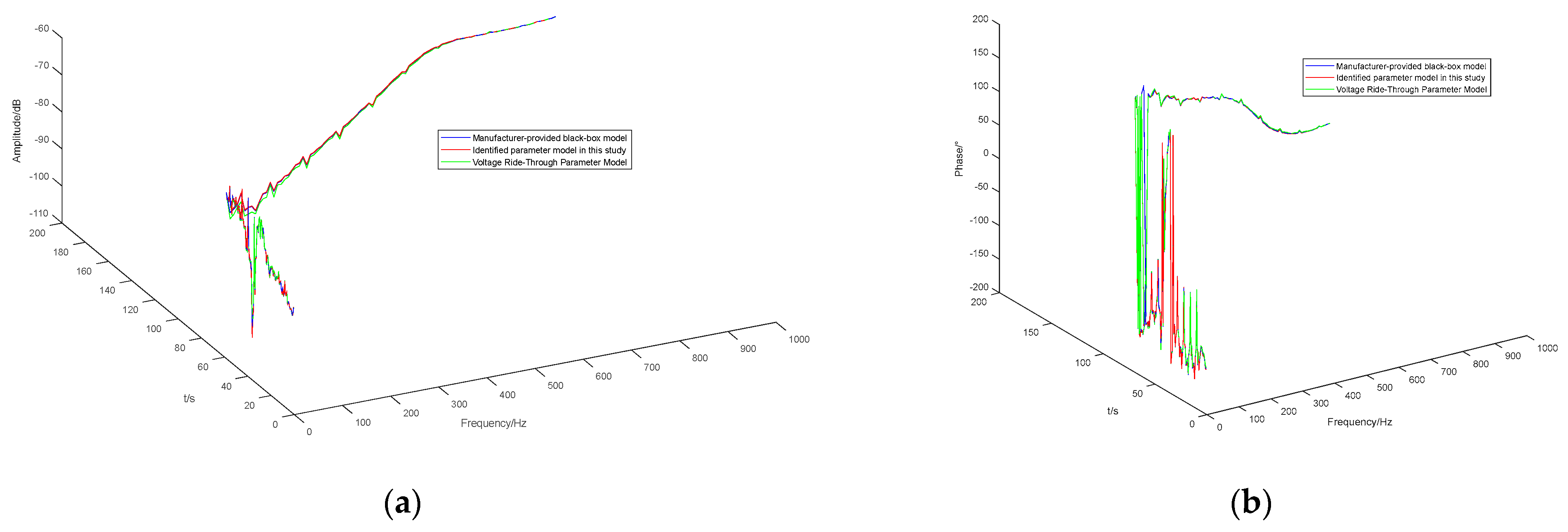
Identification based on voltage ride-through characteristics

In the traditional method identification process, from a time-domain perspective, it is necessary to sample the voltage sag and recovery process based on the actual sampling step. In this paper’s simulation process, the sampling interval is set to 5 × 10⁻⁶ s, with a single voltage sag and recovery time of approximately 0.3 s, resulting in about 50,000 samples. To ensure the accuracy of the high and low voltage ride-through identification parameters, all sampling data are involved in the intelligent algorithm iteration process.

(2)

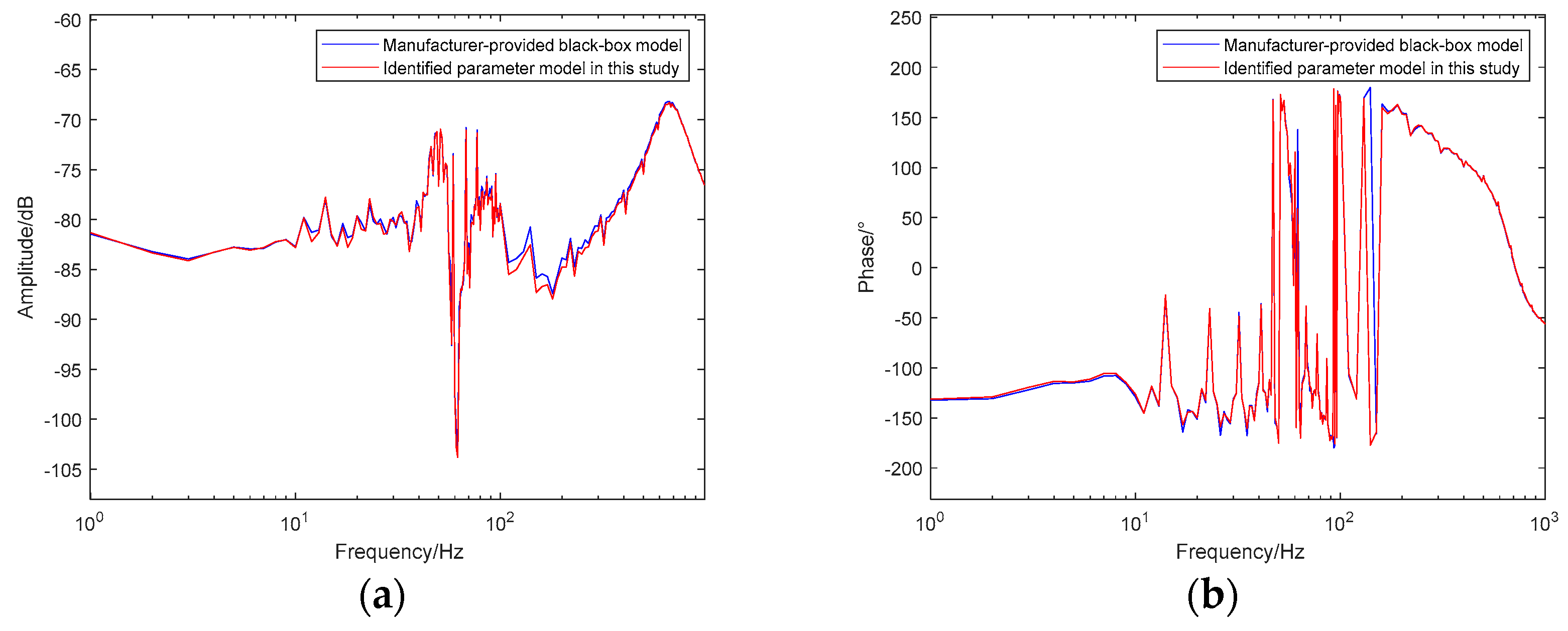
Identification based on impedance characteristics

In the parameter identification method based on impedance characteristics in this paper, it is necessary to sample and calculate the error in the frequency domain over the entire frequency range of 1–1000 Hz, with 1000 samples per iteration. Furthermore, in the proposed frequency-band-based identification method, high-frequency bands are selected to identify parameters k_{p_v} and k_{p_idg}, while medium and low-frequency bands are selected to identify parameters k_{i_v} and k_{i_idg}. This approach reduces the number of samples per iteration to 500, significantly reducing the time required for each iteration.

Taking the experimental process in this paper as an example, although the traditional identification method involves a large amount of sampling data and a complex iterative process, it allows for obtaining all the sampling data through successive simulations. The parameter identification method based on impedance characteristics requires fewer sampling data and has a simpler iterative process, but multiple simulations are needed to obtain all the sampling data. According to the simulation timing, the full-band identification method requires approximately 2 h to identify the control parameters, while using the frequency-band-based identification method proposed in this paper, the time can be reduced to under 1 h, significantly saving operating time costs.

5.2. Semi-Physical Simulation Verification with Manufacturer’s Actual Controller

In addition to the electromagnetic model simulation verification mentioned above, relevant engineering experiments have been added to further validate the effectiveness of the proposed method. Therefore, using the semi-physical simulation platform provided by the laboratory, the manufacturer’s 225 kW photovoltaic controller was operated, and its inverter control parameters were identified. The semi-physical simulation platform is shown in Figure 15.

Figure 16 presents the impedance characteristic comparison across the full frequency range between the manufacturer’s actual controller and the model identified using the proposed method.

By comparing the two sets of impedance characteristic curves, it is observed that in the newly added semi-physical simulation experiment using the manufacturer’s actual controller, the amplitude-frequency and phase-frequency characteristics obtained through the proposed parameter identification method show only small deviations from those of the actual controller across the entire frequency range, with the curves being largely consistent. This verifies the accuracy and effectiveness of the proposed method in practical engineering applications.

6. Conclusions

To address the lack of parameter identification research applicable to sub/super-synchronous oscillation scenarios, this paper constructs a mathematical model suitable for sub/super-synchronous oscillations, analyzes the sensitivity of converter control parameters, and identifies the dominant parameters in different frequency bands. Based on this, a frequency-based parameter identification method is proposed, which can quickly and accurately converge without relying on a specific optimization algorithm. Finally, comparative tests demonstrate that, under sub/super-synchronous oscillation scenarios, the effectiveness of the proposed method, its wide applicability to different intelligent algorithms, and its robustness under uncertain conditions such as environmental factors and grid frequency variations have been verified. During the simulation process, the identification errors for the parameters k_{i_v}, k_{i_idg}, k_{p_v}, and k_{p_idg} using the proposed method were 2.36%, 0.7%, 4.3%, and 3.97%, respectively, which are smaller than the errors of other identification methods in the paper, indicating higher identification accuracy. Additionally, while the traditional identification method requires approximately 2 h to identify the control parameters, the proposed frequency-segmented identification method reduces the time to under 1 h, significantly saving operational time and costs.

References

1. Li, Y.; Fan, L.; Miao, Z. Wind in weak grids: Low-frequency oscillations, sub-synchronous oscillations, and torsional interactions. IEEE Trans. Power Syst. 2020, 35, 109–118. [Google Scholar] [CrossRef]
2. Yang, C.; Ye, X. Analysis of the Development Situation of Distributed Photovoltaics in China. In Proceedings of the 2024 6th International Conference on Power and Energy Technology (ICPET), Beijing, China, 12–15 July 2024. [Google Scholar] [CrossRef]
3. Jiang, Q.R.; Wang, Y.Z. Overview of the Analysis and Mitigation Methods of Electromagnetic Oscillations in Power Systems with High Proportion of Power Electronic Equipment. Proc. CSEE 2020, 40, 7185–7201. [Google Scholar]
4. Duan, J.; Shi, D.; Diao, R.; Li, H.; Wang, Z.; Zhang, B.; Bian, D.; Yi, Z. Deep-reinforcement-learning-based autonomous voltage control for power grid operations. IEEE Trans. Power Syst. 2019, 35, 814–817. [Google Scholar] [CrossRef]
5. Shafiullah, M.; Ahmed, S.D.; Al-Sulaiman, F.A. Grid Integration Challenges and Solution Strategies for Solar PV Systems: A Review. IEEE Access 2022, 10, 52233–52257. [Google Scholar] [CrossRef]
6. Yang, D.Z.; Wang, L.P.; Zhang, J.; Wu, X.Q. Modeling of the large-scale distributed power supply and the analysis of grid-connected characteristics—(I) Photovoltaic plant thematic. Power Syst. Prot. Control. 2010, 38, 104–110. [Google Scholar]
7. Blaabjerg, F.; Teodorescu, R.; Liserre, M.; Timbus, A. Overview of control and grid synchronization for distributed power generation systems. IEEE Trans. Ind. Electron. 2006, 53, 1398–1409. [Google Scholar] [CrossRef]
8. Xiao, X.N.; Luo, C.; Liao, K.Y. Review of the Research on Subsynchronous Oscillation Issues in Electric Power System with Renewable Energy Sources. Trans. China Electrotech. Soc. 2017, 32, 85–97. [Google Scholar]
9. Xue, A.C.; Fu, X.Y.; Qiao, D.K.; Wang, Y.J.; Wang, J.W. Review and prospect of research on sub-synchronous oscillation mechanism for power system with wind power participation. Electr. Power Autom. Equip. 2020, 40, 118–128. [Google Scholar]
10. Xie, X.R.; Liu, H.K.; He, J.B.; Liu, H.; Liu, W. On New Oscillation Issues of Power Systems. Proc. CSEE 2018, 38, 2821–2828+3133. [Google Scholar]
11. Adams, J.; Carter, C.; Huang, S.H. ERCOT Experience with sub-synchronous control interaction and proposed remediation. In Proceedings of the PES T&D, Orlando, FL, USA, 7–10 May 2012; pp. 1–5. [Google Scholar]
12. Shair, J.; Xie, X.R.; Wang, L.P.; Liu, W.; He, J.B.; Liu, H. Overview of emerging subsynchronous oscillations in practical wind power systems. Renew. Sustain. Energy Rev. 2019, 99, 159–168. [Google Scholar] [CrossRef]
13. Zhan, S.Q.; Wang, N.; Li, R.; Gao, B.F.; Shao, B.B.; Song, S.H. Sub-synchronous control interaction between direct-drive PMSG-based wind farms and compensated grids. Int. J. Electr. Power Energy Syst. 2019, 109, 609–617. [Google Scholar]
14. Liang, X.; Karim, C.A.-B. Harmonics and Mitigation Techniques Through Advanced Control in Grid-Connected Renewable Energy Sources: A Review. IEEE Trans. Ind. Appl. 2018, 54, 3100–3111. [Google Scholar] [CrossRef]
15. Xiong, X.Y.; Fu, H.J.; Xiong, H.Q.; Han, Y.S.; Sun, H.S.; Li, X.M. Risk Assessment Method for the Oscillation of Renewable Energy Grid-connected System Based on Frequency Domain Impedance. High Volt. Eng. 2024, 50, 3745–3758. [Google Scholar]
16. Xiong, L.S.; Liu, X.K.; Zhuo, F.; Xie, Y.F.; Zhu, M.H.; Zhang, H.L. Small-Signal Modeling of Photovoltaic Power Generation System and Global Optimal Design for Its Controller Parameters. Power Syst. Technol. 2014, 38, 1234–1241. [Google Scholar]
17. Shen, X.W.; Zheng, J.H.; Zhu, S.Z.; Zhu, L.Z.; Shi, T.; Qu, L.N. A dq axis decoupling parameter identification strategy for grid connected inverter controller of photovoltaic generation system. Autom. Electr. Power Syst. 2014, 38, 38–43. [Google Scholar]
18. Xu, H.S.; Zeng, X.J.; Zhang, X.J.; Li, Y.R.; Xue, F.; Huang, Y.Z.; Li, C.Y. Multi-objective Step-by-step Identification Method of Control Parameters for DFIG Grid Side Converter Based on RT-LAB. Power Syst. Technol. 2025, 49, 771–780. [Google Scholar]
19. Qi, Z.H.; Duan, J.D.; Gao, T.; Deng, J.; Zhang, Y.; Chen, J. Stepwise Identification Method of Converter Control Parameters for Doubly-Fed Induction Generators. Acta Energiae Solaris Sin. 2024, 45, 18–26. [Google Scholar]
20. Ding, M.; Zhong, L.H.; Han, P.P.; Zhu, Q.L.; He, J. A practical method for parameter identification of wind power converter control link based on genetic algorithm. Electr. Technol. 2016, 35, 46–52+57. [Google Scholar]
21. Shi, R.C.; Wang, Y.H.; Shu, D.W. Identification and Modeling Method of Direct Drive Wind Farm Converter Based on Likelihood Profile Analysis. Electr. Autom. 2022, 44, 16–19. [Google Scholar]
22. Wang, F.; Yu, S.J.; Su, J.H.; Shen, Y.L. Research on Photovoltaic Grid-Connected Power System. Trans. China Electrotech. Soc. 2005, 26, 72–74+91. [Google Scholar]
23. Dash, P.P.; Kazerani, M. Dynamic Modeling and Performance Analysis of a Grid-Connected Current-Source Inverter-Based Photovoltaic System. IEEE Trans. Sustain. Ener. 2011, 2, 443–450. [Google Scholar] [CrossRef]
Figure 1. Topology of bipolar photovoltaic power generation unit.
Energies 18 03118 g001
Figure 2. Current inner loop voltage outer commutation topology.
Energies 18 03118 g002
Figure 3. (a) Admittance magnitude-frequency characteristic comparison chart; (b) Admittance phase-frequency characteristic comparison chart; (c) Parameter sensitivity chart.
Energies 18 03118 g003
Figure 4. (a) Admittance magnitude-frequency characteristic comparison chart; (b) Admittance phase-frequency characteristic comparison chart; (c) Parameter sensitivity chart.
Energies 18 03118 g004
Figure 5. (a) Admittance magnitude-frequency characteristic comparison chart; (b) Admittance phase-frequency characteristic comparison chart; (c) Parameter sensitivity chart.
Energies 18 03118 g005
Figure 6. (a) Admittance magnitude-frequency characteristic comparison chart; (b) Admittance phase-frequency characteristic comparison chart; (c) Parameter sensitivity chart.
Energies 18 03118 g006
Figure 7. (a) Admittance magnitude-frequency characteristic comparison chart; (b) Admittance phase-frequency characteristic comparison chart; (c) Parameter sensitivity chart.
Energies 18 03118 g007
Figure 8. (a) Admittance magnitude-frequency characteristic comparison chart; (b) Admittance phase-frequency characteristic comparison chart; (c) Parameter sensitivity chart.
Energies 18 03118 g008
Figure 9. Parameter identification process.
Energies 18 03118 g009
Figure 10. (a) Admittance magnitude-frequency characteristic comparison chart; (b) Admittance phase-frequency characteristic comparison chart.
Energies 18 03118 g010
Figure 11. Error diagram of the results of each parameter identification method.
Energies 18 03118 g011
Figure 12. Comparison chart of convergence speed.
Energies 18 03118 g012
Figure 13. (a) Admittance magnitude-frequency characteristic comparison chart; (b) Admittance phase-frequency characteristic comparison chart.
Energies 18 03118 g013
Figure 14. (a) Admittance magnitude-frequency characteristic comparison chart; (b) Admittance phase-frequency characteristic comparison chart.
Energies 18 03118 g014
Figure 15. Semi-physical simulation platform.
Energies 18 03118 g015
Figure 16. (a) Admittance magnitude-frequency characteristic comparison chart; (b) Admittance phase-frequency characteristic comparison chart.
Energies 18 03118 g016