Data Flow Forecasting for Smart Grid Based on Multi-Verse Expansion Evolution Physical–Social Fusion Network

Abstract

The accurate forecasting of financial flow data in power-grid operations is critical for improving operational efficiency. To tackle the challenges of low forecasting accuracy and high error rates caused by the long sequences, nonlinearity, and multi-scale and non-stationary characteristics of financial flow data, a forecasting model based on multi-verse expansion evolution (MVE²) and spatial–temporal fusion network (STFN) is proposed. Firstly, preprocess data for power-grid financial flow data based on the autoregressive integrated moving average (ARIMA) model. Secondly, establish a financial flow data forecasting framework using MVE²-STFN. Then, a feature extraction model is developed by integrating convolutional neural networks (CNN) for spatial feature extraction and bidirectional long short-term memory networks (BiLSTM) for temporal feature extraction. Next, a hybrid fine-tuning method based on MVE² is proposed, exploiting its global optimization capability and fast convergence speed to optimize the STFN parameters. Finally, the experimental results demonstrate that our approach significantly reduces forecasting errors. It reduces RMSE by 5.75% and 13.37%, MAPE by 22.28% and 41.76%, and increases R² by 1.25% and 6.04% compared to CNN-BiLSTM and BiLSTM models, respectively. These results confirm the model’s effectiveness in improving both accuracy and efficiency in financial flow data forecasting for power grids.

1. Introduction

Power grid financial flow refers to the movement and allocation of funds across various stages of power generation, transmission, and consumption during the operation of the power grid. In this paper, “financial flow data” refer specifically to the quantitative records of financial transactions associated with power grid operations. They include electricity purchase payments, transmission and distribution costs, equipment maintenance expenditures, and other monetary flows that occur across the stages of generation, transmission, and consumption. These data serve as key indicators of the grid’s operational performance, cost structure, and economic efficiency. This includes a range of financial transactions, such as electricity purchase costs, transmission and distribution expenses, and maintenance expenditures, and serves as a critical indicator of the operation efficiency and economic performance of the power grid [1]. Financial flow data are characterized by long sequences, nonlinearity, multi-scale dynamics, and non-stationarity, exhibiting complex data structures, strong volatility, and the coexistence of periodic and trend-based patterns. Forecasting power grid financial flow data not only helps power grid companies optimize financial management and improve resource scheduling efficiency, but also provides a reliable foundation for developing cost control and risk warning strategies, thereby ensuring the economic sustainability and reliability of grid operations [2,3]. The autoregressive integrated moving average (ARIMA) model is a widely used tool for time-series forecasting. It has extensive applications in data forecasting [4,5]. However, due to the dynamic nature of financial flow data, which can vary across different time periods and external environments, single accurate modeling and forecasting pose significant challenges [6].

In recent years, deep learning techniques and methods have made substantial advancements in time-series forecasting, with convolutional neural networks (CNNs) gaining widespread attention for their strengths in extracting local features [7]. In ref. [8], Mehtab et al. and colleagues conducted a comprehensive analysis of stock price time series utilizing a CNN model, demonstrating its excellent performance in capturing short-term patterns. In ref. [9], Staffini proposed a CNN architecture with extended convolutional layers to process macroeconomic time-series data, enhancing its ability to model diverse long-sequence features. In ref. [10], a convolutional neural network was applied to enterprise financial risk management. It proposed a binary classification prediction model of financial risk dilemma based on one-dimensional convolution and the sparse attention mechanism. These studies demonstrate the potential of CNNs in time-series modeling, but their ability to capture global dependencies in long sequences remains limited.

To overcome the limitations of CNNs in modeling temporal dependencies, long short-term memory (LSTM) networks have emerged as a mainstream approach for time-series modeling due to their ability to capture long-term dependencies [11]. In ref. [12], Zhao et al. proposed an LSTM model integrated with multi-attention mechanisms for stock price forecasting, significantly improving the accuracy of complex dynamic time series forecasting. In ref. [13], the LSTM was enhanced by incorporating a dynamic gating mechanism, which made it more effective in capturing long-sequence dependencies and critical temporal information. However, the unidirectional processing of LSTM overlooks the integrity of bidirectional contextual information, reducing the accuracy of power grid financial flow data forecasting and hindering effective financial management.

Bidirectional long short-term memory networks (BiLSTMs) leverage both forward and backward computations to capture contextual information in time-series simultaneously, demonstrating excellent performance in complex dynamic modeling. In ref. [14], a BiLSTM model was proposed to enhance the robustness and adaptability of financial time-series forecasting by modeling bidirectional dependencies. In ref. [15], W. Jian et al. proposed a Bi-LSTM neural network with an attention mechanism which can discern long-range relationships and sequential patterns in text data. These studies highlight that BiLSTMs outperform unidirectional LSTMs in handling complex patterns, but their higher computational complexity imposes greater demands on parameter optimization.

Despite the progress made in financial flow data forecasting, several challenges remain. The main challenges of this paper are summarized as follows:

• A single network cannot accurately extract the temporal and spatial features of financial flow data: The financial flow data of a power grid exhibit characteristics such as long sequences, nonlinearity, multi-scale patterns, and non-stationarity. While CNNs excel at capturing local features, they lack the ability to perceive global information. On the other hand, BiLSTMs can handle forward and backward dependencies in time series but show limitations in modeling nonlinear and complex patterns. Existing standalone networks cannot effectively integrate the spatial and temporal features of financial flow data, leading to lower forecasting accuracy for power grid financial flows [16].
• The ineffective training of model parameters increases the risk of the optimization process converging to local optima: Deep learning models like CNNs and BiLSTMs involve numerous parameters that significantly affect their forecasting performance. Current approaches for parameter optimization in deep learning models fail to achieve global parameter search, causing models to frequently converge to local optima during training. This limitation severely affects the efficiency and accuracy of financial flow forecasting in power grids.

To address the aforementioned challenges, a financial flow data forecasting algorithm based on multi-verse expansion evolution (MVE²) and spatial–temporal fusion network (STFN) is proposed. First, the power grid financial flow dataset is preprocessed based on the ARIMA model to construct a dataset with multi-feature dimensions and strong trend capture. Next, a financial flow data feature extraction model for power grids based on STFN is introduced, leveraging CNN to extract spatial features and BiLSTM to capture the temporal sequence features of financial flow data. This approach organically combines the spatial extraction capability of CNN and the temporal modeling strength of BiLSTM to achieve complementary advantages. Subsequently, a hybrid network fine-tuning method based on MVE² is proposed, integrating MVE² with STFN. The parameters of STFN are treated as optimization variables, and MVE² is utilized to search for the optimal parameter combination. Finally, the financial flow forecasting results are generated through pooling layers and fully connected layers. The main contributions of this paper are summarized as follows:

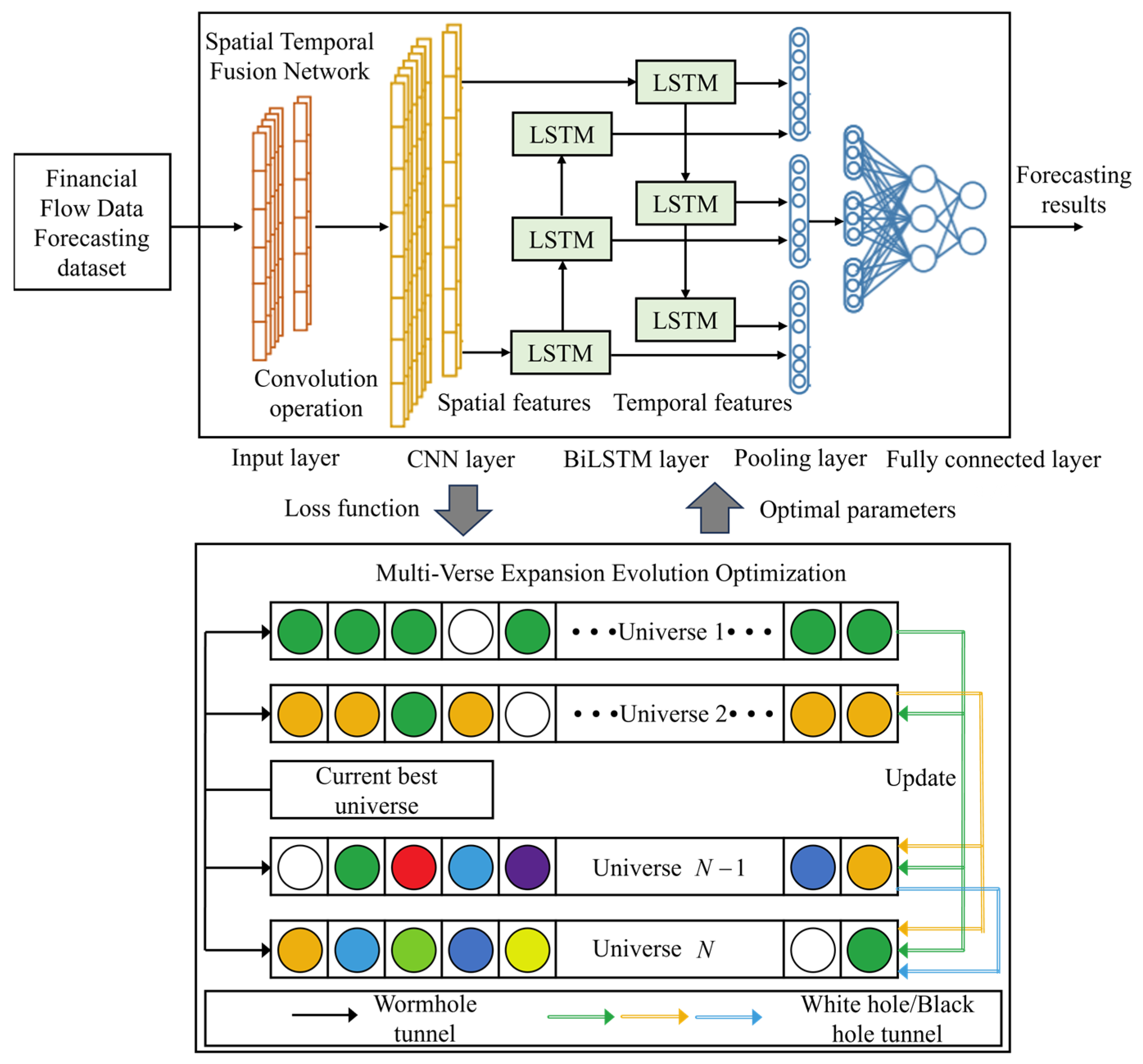
• A financial flow data feature extraction model for power grid based on STFN is proposed: This model organically combines the associative feature extraction capabilities of CNN with the temporal sequence modeling capabilities of BiLSTM. CNN effectively extracts features from the financial flow data of power grid companies, while BiLSTM captures the contextual temporal relationships. The complementary strengths of CNN and BiLSTM are leveraged, significantly improving the accuracy of power-grid financial flow data forecasting.
• A fine-tuning method for STFN based on MVE² is proposed: Leveraging the global search capability and fast convergence of MVE², it is employed to optimize the parameters of STFN. The proposed algorithm effectively mitigates the issue of traditional methods falling into local optima during model training, accelerates convergence, and significantly enhances both the efficiency and accuracy of financial flow forecasting models.

2. Data Preprocessing for Power Grid Financial Flow Data Based on ARIMA Model

2.1. Data Cleaning and Normalization Processing

The raw power grid financial flow dataset may contain a significant number of missing or anomalous values, which can severely interfere with the model’s forecasting results. Therefore, it is essential to perform imputation on the raw dataset [17]. Given the continuity characteristic of power grid financial flow data, the weighted moving average method is selected for handling missing values, expressed as

$${\tilde{x}}_t={\displaystyle \sum _{i=1}^I{v}_{t-i}{x}_{t-i}}$$

(1)

$${\displaystyle \sum _{i=1}^I{v}_{t-i}}=1$$

(2)

where ${\tilde{x}}_t$ represents the power grid financial flow data in slot $t$ imputed using the weighted moving average method. $x_t$ represents the power grid financial flow data in slot $t$. $v_t$ indicates the moving average weight of the financial flow data. $I$ is the moving average step size.

Furthermore, to accelerate the gradient descent process during model training and improve convergence speed, all data in the power grid financial flow dataset are normalized and mapped to the $[0, 1]$ range, as expressed by

$$x_t\leftarrow {\displaystyle \frac{x_t-x_{\min }}{x_{\max }-x_{\min }}}$$

(3)

where $x_{\min }$ and $x_{\max }$ denote the minimum and maximum values within the dataset, respectively. The normalized power grid financial flow data are then mapped to the range $[0, 1]$, as given by $x_t\in [0, 1]$.

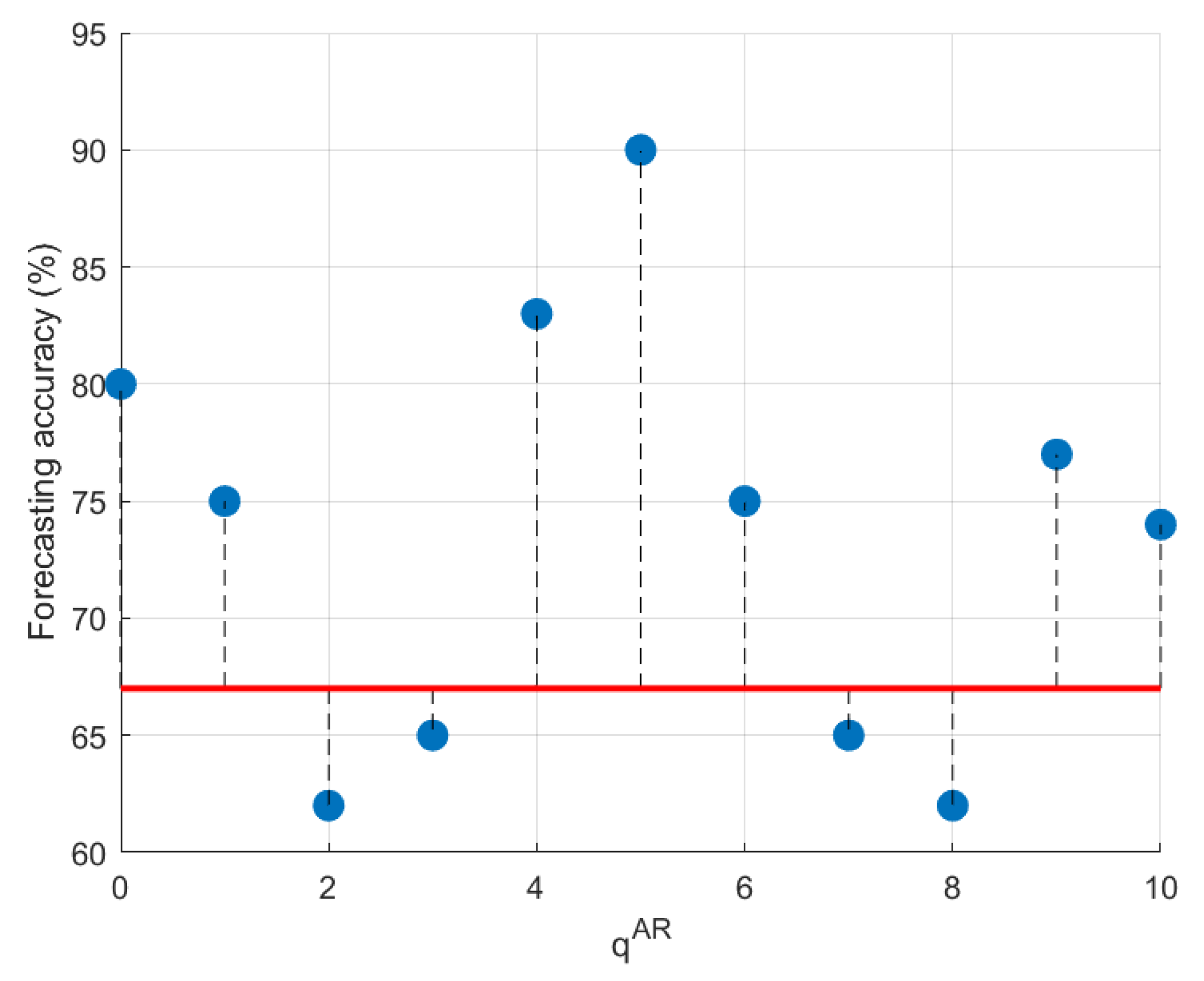
2.2. Construction of Financial Flow Data Forecasting Dataset Based on ARIMA Model

The raw grid financial flow dataset only provides surface information on financial flows and lacks the refinement of deeper features such as trends and periodicity inherent in the data. In this section, the raw grid financial flow data are modeled based on the ARIMA model. The forecasting is performed on the grid financial flow data in order to construct a dataset with multi-feature dimensions and strong trend capture, which can help the deep network to better learn and predict the general direction of future financial flows. The construction of a financial flow data forecasting dataset based on ARIMA model includes white noise test and removal, ARIMA model-based financial flow data forecasting and dataset construction.

2.2.1. White Noise Test and Removal

The financial flow data forecasting process applies the ARIMA model, which has higher requirements for the experimental data, i.e., no white noise data interference, so before the experiments are carried out, it is necessary to carry out a certain amount of pre-processing of the experimental data, i.e., white noise test and removal. The white noise test rule can be expressed as

$$\begin{array}{c}\left\{\begin{array}{cc}\xi ={\displaystyle \frac{{\displaystyle \sum } x_t}{7\times 〈{\psi }_0〉}}& \\ \left\{\begin{array}{ccc}\xi \ge {\mathsf{\Psi }}^0& \mathrm{have} \mathrm{white} \mathrm{noise}& \\ \xi <{\mathsf{\Psi }}^0\hfill & \mathrm{no} \mathrm{white} \mathrm{noise}& \end{array}\right.& \end{array}\right.\end{array}$$

(4)

where $〈{\psi }_0〉$ is the white noise auxiliary test factor. $\xi$ Indicates the value of the white noise test for financial flow data. ${\mathsf{\Psi }}^0$ is the white noise test threshold.

When the white noise test of financial flow data fails, i.e., there is a white noise situation, the filtering method is applied to the experimental data to remove the white noise, and the expression is:

$$x_t^{″}={\displaystyle \frac{x_t\times {\mu }^l}{I_t}}$$

(5)

where $x_t^{″}$ denotes the experimental data after white noise removal treatment; ${\mu }^l$ denotes the white noise filtering factor; $I_t$ denotes the standardized unit amount of the experimental data.

2.2.2. ARIMA Model-Based Financial Flow Data Forecasting and Dataset Construction

To construct a financial flow data forecasting model, the collected historical time-series data are decomposed based on a multiplicative model with the expression.

$${\tilde{x}}_t={\tilde{x}}_{t,1}+{\tilde{x}}_{t,2}+{\tilde{x}}_{t,3}+{\tilde{x}}_{t,4}+{\tilde{x}}_{t,5}$$

(6)

where ${\tilde{x}}_t$ is financial flow data time-series data. ${\tilde{x}}_{t,1}$ represents trend components of the historical financial flow data sequence. ${\tilde{x}}_{t,2}$ indicates the historical temperature fluctuation sequence. ${\tilde{x}}_{t,3}$ indicates the historical economic development sequence. ${\tilde{x}}_{t,4}$ indicates the historical business development sequence; ${\tilde{x}}_{t,5}$ indicates the historical random chance components sequence.

The structure of the ARIMA model can be expressed as $\mathrm{ARIMA}\left(p^{\mathrm{AR}}, d^{\mathrm{AR}}, q^{\mathrm{AR}}\right)$, where the order of the autoregressive term $p^{\mathrm{AR}}$ indicates that the model depends on data from the previous $p^{\mathrm{AR}}$ time point. $d^{\mathrm{AR}}$ is the order of the difference, which is used to convert non-stationary data to stationary data. $q^{\mathrm{AR}}$ is the order of the sliding average term, which indicates that the model depends on the error term at the previous $q^{\mathrm{AR}}$ time point. The forecast of financial flow data based on ARIMA model can be expressed as follows

$${\widehat{x}}_{t,d^{\mathrm{AR}}}=\left\{\begin{array}{c}{\left(1-\beta \right)}^d{\tilde{x}}_t\\ {\chi }_1{\widehat{x}}_{t-1,d^{\mathrm{AR}}}+{\chi }_2{\widehat{x}}_{t-2,d^{\mathrm{AR}}}+\dots +{\chi }_{q^{\mathrm{AR}}}{\widehat{x}}_{t-q^{\mathrm{AR}},d^{\mathrm{AR}}}+\delta \end{array}\right.$$

(7)

where ${\widehat{x}}_{t,d^{\mathrm{AR}}}$ is the financial flow data in the financial flow data after the $d^{\mathrm{AR}}$-th sub-differential, the composition of the time series of smooth data. $\beta$ represents the financial flow data lag operator. ${\chi }_i$ represents the autoregressive coefficient. $\delta$ represents a constant, assuming the financial flow data forecasting results of the function of error adjustment, and the value of the range is [0, 1].

A dataset is constructed based on the raw grid financial flow data and the financial flow data obtained from the ARIMA model forecasting. The dataset is further predicted by the MVE²-STFN so as to improve the efficiency and accuracy of the forecasting.

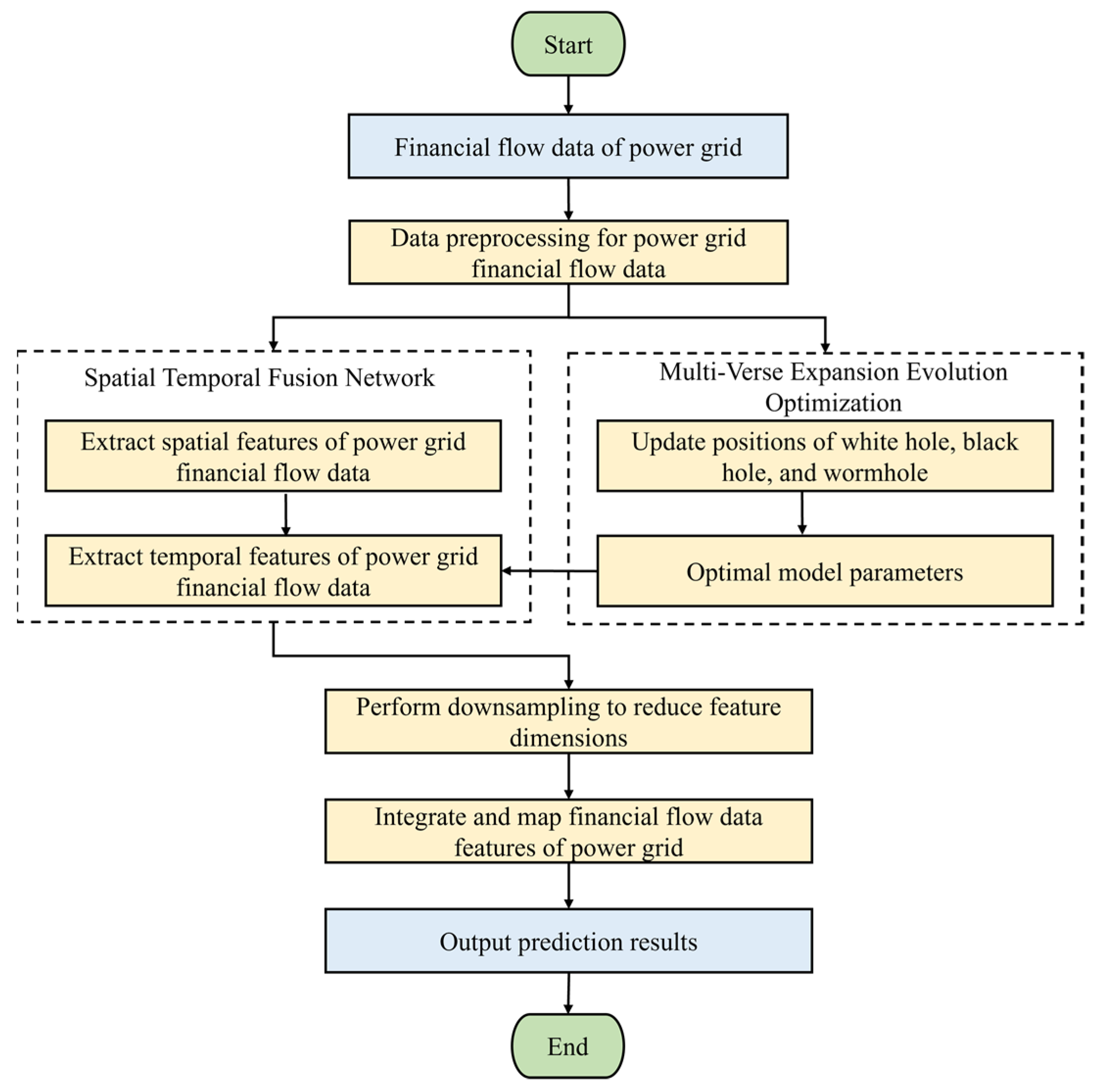
3. Financial Flow Data Forecasting Based on MVE²-STFN

To address the issues of low forecasting accuracy and high errors caused by the long sequences, nonlinearity, multi-scale, and non-stationary characteristics of power grid financial flow data, a financial flow data forecasting framework based on MVE²-STFN is proposed, as shown in Figure 1. The framework includes an input layer, CNN layer, BiLSTM layer, pooling layer, and fully connected layer. The input layer performs data cleaning and normalization on the raw power grid financial flow dataset, mitigating the impact of missing or anomalous values in the original data on the forecasting results. The CNN layer and the BiLSTM layer are used to extract spatial features and temporal sequence features of the power grid financial flow data, respectively. The pooling layer downsamples the temporal features output from the BiLSTM layer to reduce the spatial dimensions of the features, thereby enhancing the model’s generalization capability. The fully connected layer integrates and maps the spatial and temporal features of financial flow data, outputting the final forecasting results. Additionally, the MVE² algorithm is integrated with the STFN, using the STFN parameters as optimization variables for the MVE² algorithm. The MVE² algorithm is utilized to search for the optimal parameter combination, improving the forecasting accuracy and convergence speed of power grid financial flow data.

The financial flow forecasting process based on MVE²-STFN is illustrated in Figure 2. First, the power grid financial flow dataset is cleaned and normalized to eliminate the influence of missing or anomalous values on forecasting results. Next, the parameters of STFN are treated as optimization variables for the MVE² algorithm, which searches for the optimal parameter combination. Subsequently, based on the optimal parameter combination, the STFN employs CNN to extract spatial features and BiLSTM to extract temporal sequence features from the financial flow data. Finally, the pooling layer performs downsampling, while the fully connected layer combines and maps the features to generate the forecasting results for the financial flow data.

3.1. Power Grid Financial Flow Feature Extraction Model Based on STFN

Power grid financial flow data exhibit characteristics such as long sequences, nonlinearity, multi-scale variability, and non-stationarity. While CNN excels at extracting spatial features, it has limited capability to capture global information. On the other hand, BiLSTM effectively models bidirectional dependencies in temporal data but is relatively inadequate in handling the local features of financial flow data. Existing single-network architectures fail to effectively integrate the spatial and temporal features of financial flow data, leading to low forecasting accuracy. To address these issues, we propose a feature extraction model for power grid financial flow data based on STFN. The model leverages CNN to extract spatial features and BiLSTM to extract temporal features, achieving an effective integration of spatial and temporal characteristics. The detailed approach is described as follows.

First, the CNN layer receives the power grid financial flow data from the input layer and extracts its spatial features. The CNN model is made up of convolutional, pooling, and fully connected layers. Its core strength lies in its ability to effectively extract features from input data using convolutional and pooling layers. In the convolutional layers, CNN extracts local features from the data through a sequence of convolution operations. The pooling layers reduce the feature dimensions, lowering computational complexity and retaining the most significant features. CNN employs convolution operations instead of general matrix operations, significantly improving computational efficiency. This can be expressed as

$$S=X\ast W$$

(8)

where $S$ represents the feature-mapping matrix after convolution, $X$ denotes the input matrix, $W$ represents the weight matrix (i.e., the kernel function), and $\ast$ denotes the convolution operator. Since the convolution operation typically involves multidimensional input, the weight matrix is also usually multidimensional. The number of convolutional kernels determines the level of abstraction in feature extraction. Their size can be adjusted based on the data volume of the input, which can be expressed as

$$s_{p,q}={\displaystyle \sum _{l=1}^L{\displaystyle \sum _{m=1}^M{x}_{l,m}{w}_{p+l,q+m}}}$$

(9)

where $s_{p,q}$ represents the element in the $p$-th row and $q$-th column of the feature-mapping matrix $S$. $x_{l,m}$ corresponds to the element in the $l$-th row and $m$-th column of the 2D input matrix $X$, and $w_{p+l,q+m}$ is the element in the $(p+l)$-th row and $(q+m)$-th column of the 2D convolution kernel $W$. Using sparse connections and shared weights, CNN operates through convolutional and pooling layers to extract meaningful spatial feature information from power grid financial flow data.

Next, the spatial features of power grid financial flow data extracted by the CNN are input into the BiLSTM network. The forward LSTM cells process the preceding temporal dependencies, while the backward LSTM cells capture subsequent temporal dependencies. The forward LSTM layer’s memory units are used to learn temporal features from preceding contexts, while the backward LSTM layer’s memory units learn from subsequent contexts. Each LSTM cell consists of structures such as the input, forget, and output gates, along with memory cells. The parameter set of the BiLSTM network is denoted as ${\theta }^{BiLSTM}=\{{\overrightarrow{\omega }}_i,{\overrightarrow{\omega }}_f,{\overrightarrow{\omega }}_o,{\overrightarrow{\omega }}_C,{\overrightarrow{b}}_i,{\overrightarrow{b}}_f,{\overrightarrow{b}}_o,{\overrightarrow{b}}_C,{\overleftarrow{\omega }}_i,{\overleftarrow{\omega }}_f,{\overleftarrow{\omega }}_o,{\overleftarrow{\omega }}_C,{\overleftarrow{b}}_i,{\overleftarrow{b}}_f,{\overleftarrow{b}}_o,{\overleftarrow{b}}_C\}$. Specifically, ${\overrightarrow{\omega }}_i$, ${\overrightarrow{\omega }}_f$, ${\overrightarrow{\omega }}_o$, ${\overrightarrow{\omega }}_C$, ${\overrightarrow{b}}_i$, ${\overrightarrow{b}}_f$, ${\overrightarrow{b}}_o$, and ${\overrightarrow{b}}_C$ represent the weight and bias matrices for the input, forget, output gates, and memory cells in the forward LSTM cells, respectively. Similarly, ${\overleftarrow{\omega }}_i$, ${\overleftarrow{\omega }}_f$, ${\overleftarrow{\omega }}_o$, ${\overleftarrow{\omega }}_C$, ${\overleftarrow{b}}_i$, ${\overleftarrow{b}}_f$, ${\overleftarrow{b}}_o$, and ${\overleftarrow{b}}_C$ represent the corresponding matrices for the backward LSTM cells.

Then, the LSTM cells use the forget gates to determine which information in the cell state should be retained, which is expressed as

$$\left\{\begin{array}{l}{\overrightarrow{f}}_t=\sigma ({\overrightarrow{\omega }}_f\cdot [{\overrightarrow{h}}_{t-1},x_t]+{\overrightarrow{b}}_f)\\ {\overleftarrow{f}}_t=\sigma ({\overleftarrow{\omega }}_f\cdot [{\overleftarrow{h}}_{t+1},x_t]+{\overleftarrow{b}}_f)\end{array}\right.$$

(10)

where $\sigma (\cdot )$ represents the sigmoid activation function. ${\overrightarrow{h}}_{t-1}$ and ${\overleftarrow{h}}_{t+1}$ are the outputs from the previous forward and backward LSTM cells, respectively. ${\overrightarrow{f}}_t$ and ${\overleftarrow{f}}_t$ denote the forgetting degree applied to the cell state by the forget gates of the forward and backward LSTM cells, respectively.

Next, the LSTM cells determine the new information to be added through the input gate and update the cell state, which can be represented as

$$\left\{\begin{array}{l}{\overrightarrow{o}}_t=\sigma ({\overrightarrow{\omega }}_o\cdot [{\overrightarrow{h}}_{t-1},x_t]+{\overrightarrow{b}}_o)\\ {\overleftarrow{o}}_t=\sigma ({\overleftarrow{\omega }}_o\cdot [{\overleftarrow{h}}_{t+1},x_t]+{\overleftarrow{b}}_o)\end{array}\right.$$

(11)

$$\left\{\begin{array}{l}{\overrightarrow{C}}_t={\overrightarrow{f}}_t\times {\overrightarrow{C}}_{t-1}+{\overrightarrow{i}}_t\times \tanh ({\overrightarrow{\omega }}_C\cdot [{\overrightarrow{h}}_{t-1},{\overline{s}}_t]+{\overrightarrow{b}}_C)\\ {\overleftarrow{C}}_t={\overleftarrow{f}}_t\times {\overleftarrow{C}}_{t+1}+{\overleftarrow{i}}_t\times \tanh ({\overleftarrow{\omega }}_C\cdot [{\overleftarrow{h}}_{t+1},{\overline{s}}_t]+{\overleftarrow{b}}_C)\end{array}\right.$$

(12)

where ${\overrightarrow{i}}_t$ and ${\overleftarrow{i}}_t$ represent the extent to which the input gates of the forward and backward LSTM cells update the new information, respectively. ${\overrightarrow{C}}_t$ and ${\overleftarrow{C}}_t$ represent the cell states of both the forward and backward LSTM cells.

Finally, the LSTM cells determine the output through the output gate, which can be expressed as

$$\left\{\begin{array}{l}{\overrightarrow{o}}_t=\sigma ({\overrightarrow{\omega }}_o\cdot [{\overrightarrow{h}}_{t-1},x_t]+{\overrightarrow{b}}_o)\\ {\overleftarrow{o}}_t=\sigma ({\overleftarrow{\omega }}_o\cdot [{\overleftarrow{h}}_{t+1},x_t]+{\overleftarrow{b}}_o)\end{array}\right.$$

(13)

$$\left\{\begin{array}{l}{\overrightarrow{h}}_t={\overrightarrow{o}}_t\times \tanh ({\overrightarrow{C}}_t)\\ {\overleftarrow{h}}_t={\overleftarrow{o}}_t\times \tanh ({\overleftarrow{C}}_t)\end{array}\right.$$

(14)

where ${\overrightarrow{o}}_t$ and ${\overleftarrow{o}}_t$ represent the tolerance levels of the output gates in the forward and backward LSTM cell units, respectively. ${\overrightarrow{h}}_t$ and ${\overleftarrow{h}}_t$ denote the outputs from both the forward and backward LSTM cell units.

By combining the outputs of the forward and backward LSTM cell units, the final temporal feature representation of the BiLSTM network is expressed as

$$y_t=\sigma (\overrightarrow{\upsilon }\cdot {\overrightarrow{h}}_t+\overleftarrow{\upsilon }\cdot {\overleftarrow{h}}_t)$$

(15)

where $\overrightarrow{\upsilon }$ and $\overleftarrow{\upsilon }$ represent the weights of the forward and backward LSTM cell units.

3.2. Fine-Tuning Method for STFN Based on MVE²

MVE² is a heuristic optimization algorithm based on the concept of universe expansion. It offers strong global optimization capabilities, fast convergence, and minimal parameter adjustment. The parameters of STFN are treated as optimization variables for MVE². The algorithm searches for the optimal parameter combination to address the issue of traditional methods falling into local optima during model training, thereby accelerating convergence. The core idea of MVE² leverages the concepts of white holes, black holes, and wormholes in the universe to guide the search process in finding optimal solutions [18]. Each universe is treated as a candidate solution to the optimization problem, with the objects within the universe representing parameter combinations. The fitness of a candidate solution corresponds to the universe’s expansion rate. Finding the optimal universe involves iterative optimization. After initialization, multi-verse iteratively evolves to reach the optimal solution. In this study, MVE² is used to optimize the parameters $\pi =\{W,{\theta }^{BiLSTM}\}$ of the STFN, including the weight matrix $W$ of the CNN model and the parameters ${\theta }^{BiLSTM}$ of the BiLSTM model. Suppose a population consisting of $N$ universes search within a $D$-dimensional objective space, where the corresponding universe matrix for the search space can be expressed as

$$U=\left(\begin{array}{c}{u}_1\\ u_2\\ ⋮\\ u_N\end{array}\right)=\left(\begin{array}{cccc}{\pi }_1^1& {\pi }_1^2& \dots & {\pi }_1^D\\ {\pi }_2^1& {\pi }_2^2& \dots & {\pi }_2^D\\ ⋮& ⋮& \ddots & ⋮\\ {\pi }_N^1& {\pi }_N^2& \dots & {\pi }_N^D\end{array}\right)$$

(16)

where N represents the number of universes (candidate solutions), and D represents the dimension of each universe. $u_n=[{\pi }_n^1,{\pi }_n^2,\dots ,{\pi }_n^D]$ denotes the $n$-th universe. ${\pi }_n^d$ indicates the position of the $d$-th black hole in the $n$-th universe.

In the context of financial flow data prediction, the encoding of each universe represents a specific forecasting scenario. Assume there are city nodes and regional nodes, with each node and its corresponding grid parameters encoded into specific values. Each encoding scheme includes both spatial and temporal features of the grid, which are identified using natural number labels, ensuring that each feature has a unique identifier. To optimize the model’s performance, the MVE² algorithm treats these encodings as optimization variables and adjusts them, simulating the process of material exchange and expansion between multiple universes. The encoding process is as follows: first, parameters are extracted using CNN and BiLSTM models to obtain spatial and temporal features. Then, these extracted features are numbered according to specific rules to form the initial universe encodings, ensuring that each encoding corresponds to a complete forecasting scenario. Subsequently, the MVE² algorithm optimizes these encodings through global search, progressively adjusting parameters to find the optimal combination of forecasting scenarios, ultimately producing the predicted financial flow results for the grid.

In this study, MVE² is used to optimize the parameters $\pi =\{W,{\theta }^{BiLSTM}\}$ of the STFN. $W$ represents the weight matrix (i.e., the kernel function). ${\theta }^{BiLSTM}=\{{\overrightarrow{\omega }}_i,{\overrightarrow{\omega }}_f,{\overrightarrow{\omega }}_o,{\overrightarrow{\omega }}_C,{\overrightarrow{b}}_i,{\overrightarrow{b}}_f,{\overrightarrow{b}}_o,{\overrightarrow{b}}_C,{\overleftarrow{\omega }}_i,{\overleftarrow{\omega }}_f,{\overleftarrow{\omega }}_o,{\overleftarrow{\omega }}_C,{\overleftarrow{b}}_i,{\overleftarrow{b}}_f,{\overleftarrow{b}}_o,{\overleftarrow{b}}_C\}$ is the parameter set of the BiLSTM network. Specifically, ${\overrightarrow{\omega }}_i$, ${\overrightarrow{\omega }}_f$, ${\overrightarrow{\omega }}_o$, ${\overrightarrow{\omega }}_C$, ${\overrightarrow{b}}_i$, ${\overrightarrow{b}}_f$, ${\overrightarrow{b}}_o$, and ${\overrightarrow{b}}_C$ represent the weight and bias matrices for the input, forget, output gates, and memory cells in the forward LSTM cells, respectively. Similarly, ${\overleftarrow{\omega }}_i$, ${\overleftarrow{\omega }}_f$, ${\overleftarrow{\omega }}_o$, ${\overleftarrow{\omega }}_C$, ${\overleftarrow{b}}_i$, ${\overleftarrow{b}}_f$, ${\overleftarrow{b}}_o$, and ${\overleftarrow{b}}_C$ represent the corresponding matrices for the backward LSTM cells.

The MVE² algorithm employs a roulette wheel mechanism to simulate the mathematical model of white holes and black holes. Objects in different universes are transmitted through white-hole and black-hole tunnels. The roulette wheel mechanism is expressed as

$$u_n^d=\left\{\begin{array}{l}{u}_k^d, r_1<NI(u_n)\\ u_n^d, r_1\ge NI(u_n)\end{array}\right.$$

(17)

where $u_k^d$ represents the position of the $d$-th black hole in the $k$-th universe selected by the roulette wheel mechanism. $NI(u_n)$ denotes the normalized expansion rate of the $n$-th universe, and $r_1$ is a random number in the range $[0,1]$.

The travel distance rate of the object is denoted as $TDR$, which is a dynamic parameter, represented as

$$TDR=1-{\displaystyle \frac{e^{\frac{1}{\sigma }}}{E^{\frac{1}{\sigma }}}}$$

(18)

where $e$ is the current iteration number. $E$ is the preset maximum number of iterations. $\sigma$ is the adjustment coefficient, typically treated as a constant. $TDR$ dynamically adjusts the search step size by maintaining a larger value in the early stages of the algorithm to promote global exploration, then gradually decreasing the step size as iterations progress to shift toward local refinement, thereby achieving a balance between global exploration and local exploitation.

$WEP$ represents the probability of the existence of a wormhole, which is specifically expressed as

$$WEP=WE{P}^{\min }+e\cdot \left({\displaystyle \frac{WE{P}^{\max }-WE{P}^{\min }}{E}}\right)$$

(19)

where $WE{P}^{\max }$ and $WE{P}^{\min }$ represent the minimum and maximum values of the probability of the existence of a wormhole, respectively. $WEP$ employs a linearly increasing probability mechanism that sets a lower probability in the early stages to reduce random interference, then progressively increases the probability value as iterations proceed to enhance the algorithm’s ability to escape local optima.

To maintain the diversity of the multi-verse and prevent the algorithm from getting trapped in a local optimum, the positions of black holes in the optimal universe must be updated, as expressed by

$$\left\{\begin{array}{l}{\tilde{u}}_n^d+TDR\cdot \left[(b_{up}^d-b_{low}^d)\cdot r_4+b_{low}^d\right], r_3<0.5, r_2<WEP\\ {\tilde{u}}_n^d-TDR\cdot \left[(b_{up}^d-b_{low}^d)\cdot r_4+b_{low}^d\right], r_3\ge 0.5, r_2<WEP\\ {\tilde{u}}_n^d, r_2\ge WEP\end{array}\right.$$

(20)

where ${\tilde{u}}_n^d$ represents the position of the $d$-th black hole in the current optimal universe. $r_2$, $r_3$, and $r_4$ are random numbers within the range $[0,1]$. $b_{\mathrm{up}}^d$ and $b_{\mathrm{low}}^d$ denote the upper and lower boundaries of the $d$-th black hole ${\pi }_n^d$ in the $n$-th universe. By applying random perturbations to the current optimal solution based on search-space boundaries, the algorithm maintains its overall search direction while increasing population diversity, effectively preventing premature convergence to local optima.

The fitness function value is a crucial criterion for determining whether the position of an object within the current universe is optimal. In this paper, the mean squared error of the network model is chosen as the fitness function, i.e.,

$${\mathrm{Fit}}_{ \mathrm{ness}}=({\displaystyle \sum _{i=1}^n{(y_i-{\overline{y}}_i)}^2})/n$$

(21)

where $y_i$ and ${\overline{y}}_i$ represent the predicted value and the true observed value in the network prediction model, respectively.

In the early stages of the algorithm’s optimization, the distribution of object positions in the universe is random, resulting in higher dispersion and a larger standard deviation. In later stages, the objects tend to cluster around the optimal position, leading to higher concentration and a smaller standard deviation. When the standard deviation of object positions falls below a predefined reference value, the optimization process is considered complete. The decision-making formula is as follows

$$\sigma \le \epsilon$$

(22)

where $\sigma$ represents the standard deviation of all particle positions at the current time, and $\epsilon$ is the predefined small threshold value.

3.3. Limitations of the Algorithm

The proposed algorithm in this paper utilizes the global exploration ability and rapid convergence characteristics of MVE², effectively reducing the problem of traditional algorithms getting trapped in local optima during model training. This greatly improving the efficiency of power grid financial flow prediction. However, the proposed algorithm overlooks the security issue during power grid financial flow prediction. In the power grid, any tampering with or loss of financial flow data can lead to users being overcharged or undercharged, which may trigger transaction disputes and system risks. These issues can cause large-scale trust crises, resulting in severe economic and property losses. Therefore, ensuring the information security of financial flow data is crucial. For example, “Adaptive Tracking Control for Uncertain Nonlinear Multi-Agent Systems with Partially Sensor Attack” [19] highlights a key gap in the current power-system information security field—namely, the lack of attack-detection mechanisms based on output error information, which makes it challenging to detect attacks in a timely manner. Therefore, the authors propose an attack-monitoring method that combines output error detection with Nussbaum-type compensation to enhance the robustness and security of multi-agent systems under sensor attacks. “Adaptive Cooperative Fault-Tolerant Control for Output-Constrained Nonlinear Multi-Agent Systems under Stochastic FDI Attacks” [20] points out that existing information security control methods for power grids lack the consideration of real-world environmental constraints, resulting in the poor adaptability of security control strategies to practical scenarios. The aforementioned works offer valuable insights into how the proposed algorithm can be further improved, and we plan to explore these directions in future work.

4. Experimental Results and Analysis

To evaluate the effectiveness of the proposed algorithm, we select a first-tier subsidiary of a power grid as the test subject. Time-series financial flow data, collected daily from 2022 to 2024, are used to construct the dataset for model training. The collected time-series financial flow dataset is partitioned into 80% for training, 10% for validation, and 10% for testing.

Table 1. Experimental parameter settings.

Parameter	Value	Parameter	Value
Number of convolution kernels	128	Convolution kernel size	3
Training set proportion	80%	Validation set ratio	10%
Number of hidden layers	3	Initial learning rate	0.001

outlines the experimental parameter settings. The proposed MVE²-STFN model and comparative baseline algorithms are implemented using Python 3.9 with the PyTorch (PyTorch version 2.6.0) deep learning framework. All experiments are conducted on a workstation equipped with an NVIDIA RTX 3090 GPU and 128 GB of RAM. In the STFN, the CNN layer uses a single input channel with 128 convolutional kernels, each of size 3. The BiLSTM layer is configured with 128 hidden states and four stacked hidden layers to enhance the model’s capacity for handling sequential data [21]. The model training process utilizes mean square error (MSE) as the loss function, with an initial learning rate set to 0.001. A learning rate scheduler is employed to adjust the rate dynamically during training. The comparison algorithms include CNN-BiLSTM [22] and BiLSTM [23]. The CNN-BiLSTM consists of both CNN and BiLSTM layers, combining CNN’s ability to extract spatial features with BiLSTM’s capacity for sequential modeling. The CNN layers capture local spatiotemporal dependencies through convolutional kernels, while the BiLSTM’s bidirectional recurrent structure captures long-term dependencies. It uses the Adam optimizer for parameter updates but does not account for the multi-scale and non-stationary nature of power grid financial flow data. Additionally, it lacks a global optimization mechanism, limiting the parameter search to local optima. The BiLSTM consists solely of BiLSTM layers, using bidirectional gated recurrent units to model the temporal dependencies in power grid financial flow data, capturing short-term fluctuations and forecasting long-term trends. However, it does not incorporate CNN layers to extract spatial features of the power grid financial flow data or utilize the MVE² algorithm to optimize the model parameters. As a result, it fails to effectively combine the spatial and temporal features of the data, leading to lower prediction accuracy for power grid financial flows.

4.1. Evaluation Metrics

To thoroughly evaluate the algorithm’s performance in forecasting the financial flow data of the power grid, the evaluation metrics root mean square error (RMSE), mean absolute error (MAE), $R^2$-value, and mean absolute percentage error (MAPE) are employed [24,25], defined as

$$RMSE=\sqrt{{\displaystyle \frac{1}{N}}{\displaystyle \sum _{n=1}^N{(y_n-{\widehat{y}}_n)}^2}}$$

(23)

$$MAE={\displaystyle \frac{1}{N}}{\displaystyle \sum _{n=1}^N|y_n-{\widehat{y}}_n|}$$

(24)

$$MAPE=1-{\displaystyle \frac{{\displaystyle \sum _{n=1}^N{(y_n-{\widehat{y}}_n)}^2}}{{\displaystyle \sum _{n=1}^N{(\overline{y}-{\widehat{y}}_n)}^2}}}$$

(25)

$$R^2={\displaystyle \frac{\frac{1}{N}{\displaystyle \sum _{n=1}^N|y_n-{\widehat{y}}_n|}}{y_n}}$$

(26)

where $N$ represents the forecasting step length. $y_n$ and ${\widehat{y}}_n$ denote the actual and forecasting values of the financial flow data at step $n$, respectively. $\overline{y}$ represents the mean of the actual financial flow values.

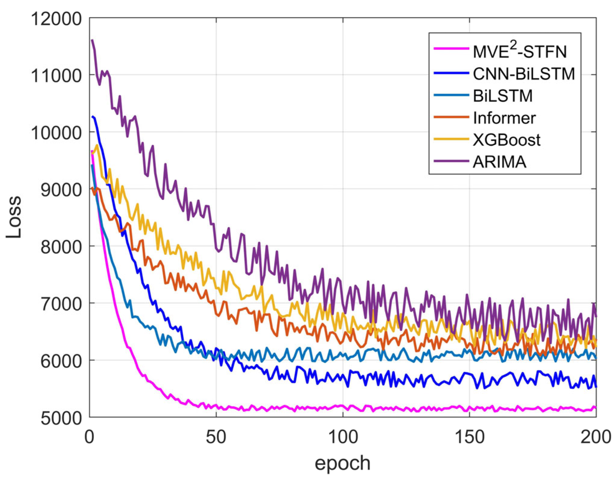
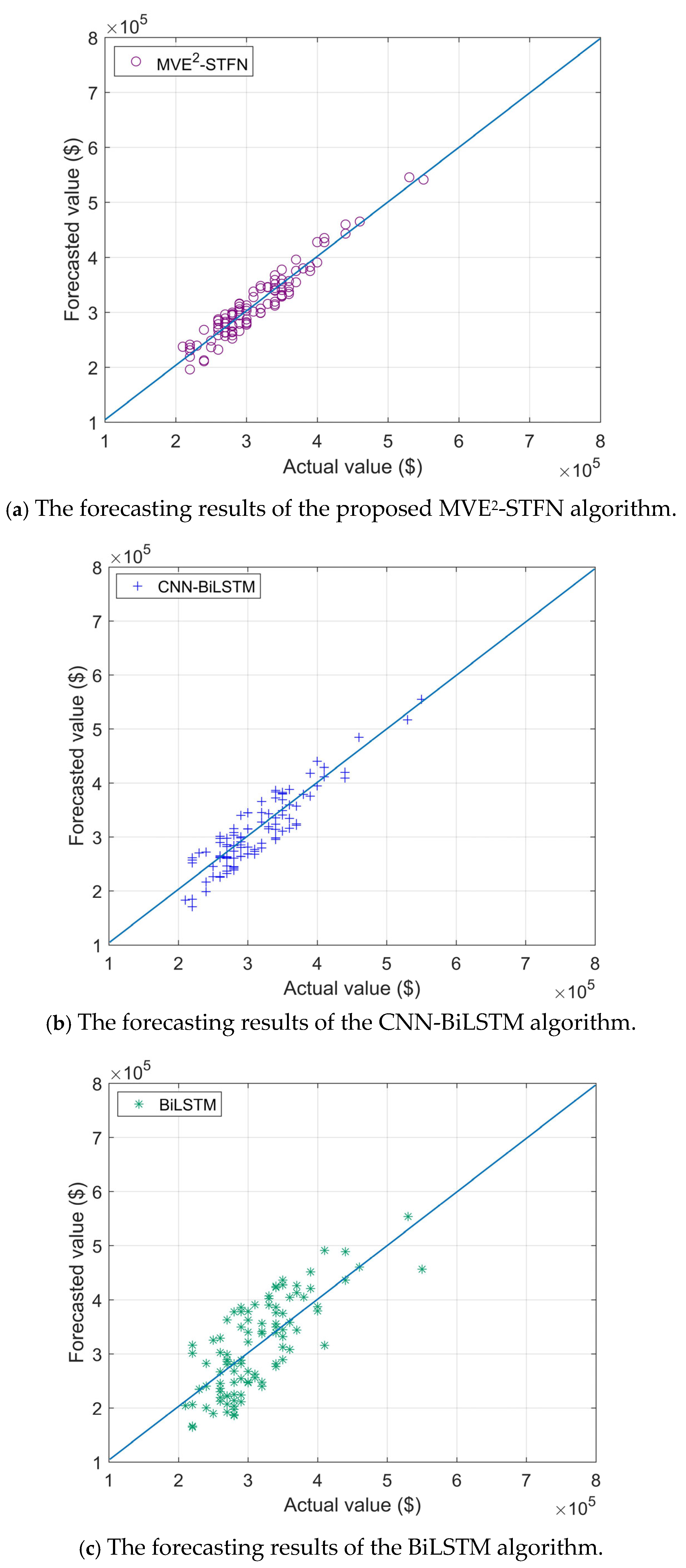
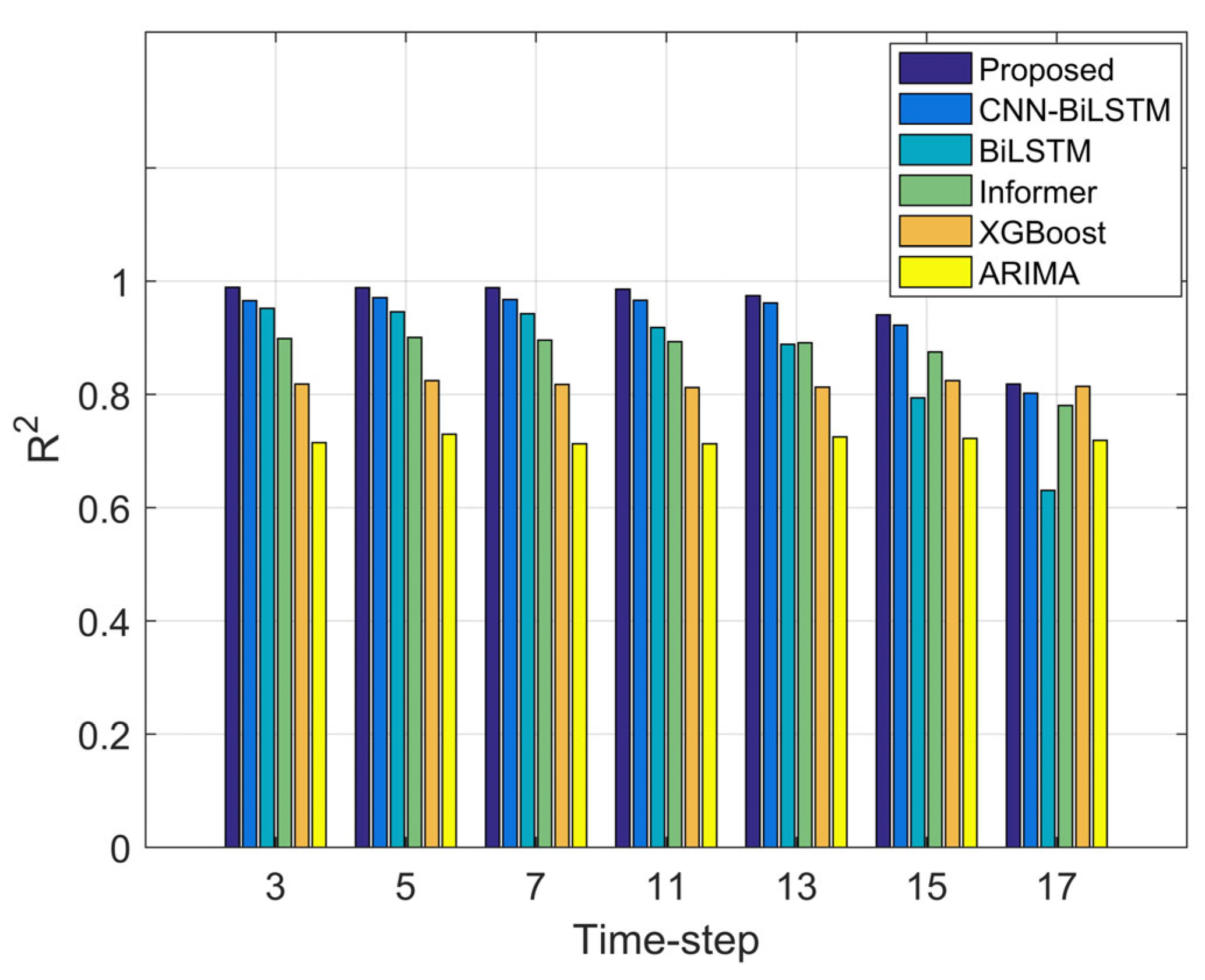
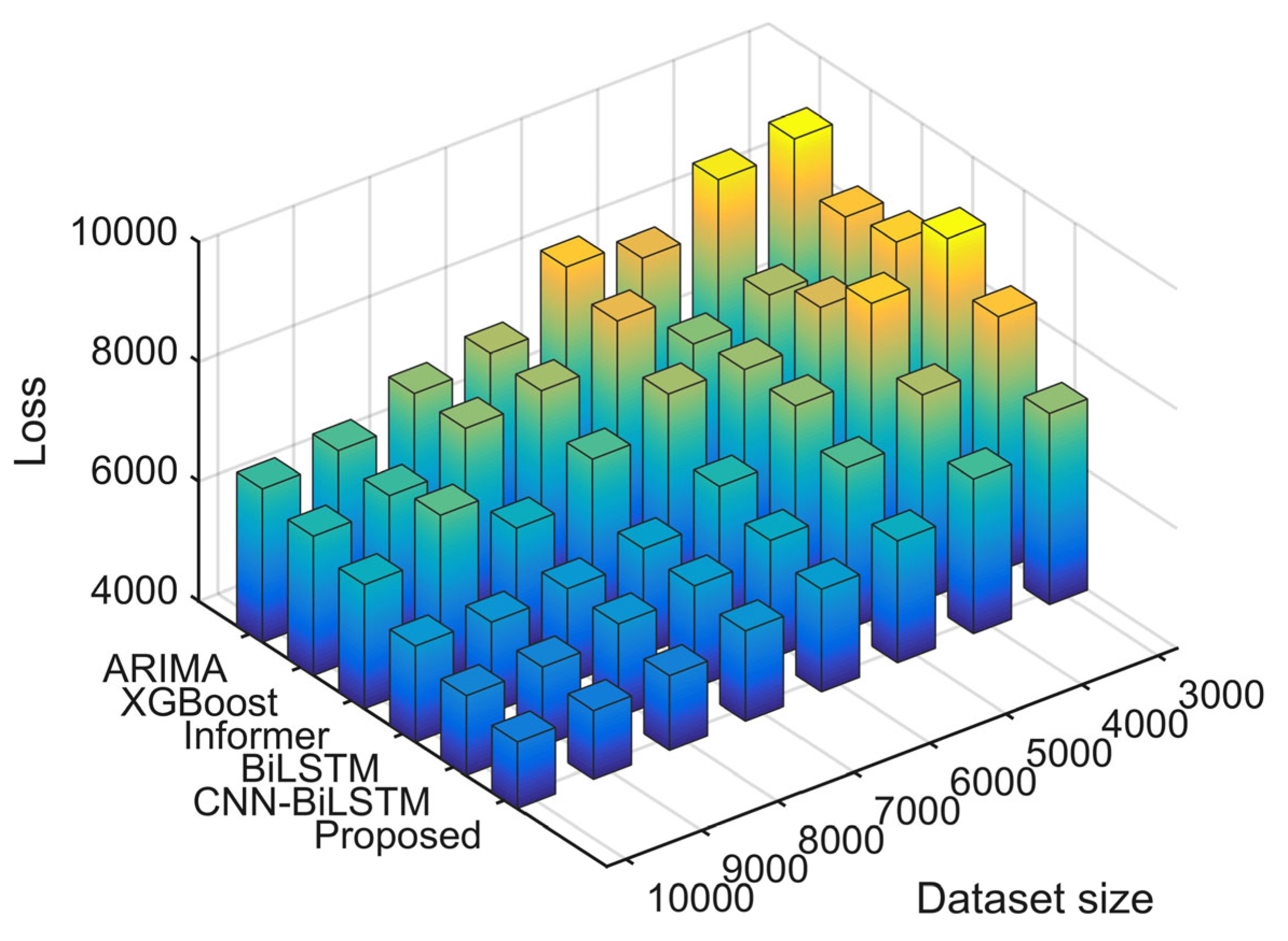
4.2. Experimental Results

Figure 3 shows the variation in the ARIMA model forecasting accuracy versus moving average order. Moving average order $q^{\mathrm{AR}}$ is directly related to the accuracy of the model forecasting. Therefore, it is necessary to determine the order of the ARIMA model before generating the dataset using the ARIMA model. The simulation results show that when the value of the moving average order $q^{\mathrm{AR}}$ is 5, the forecasting accuracy reaches the maximum value of 89%. Therefore, the optimal value of the moving average order $q^{\mathrm{AR}}$ is determined to be 5.

Figure 4 illustrates the variation in loss function across epochs for different algorithms. The loss function can be measured by RMSE. As training progresses, the loss functions of the proposed MVE²-STFN, CNN-BiLSTM, and BiLSTM algorithms all show a rapid initial decline followed by stabilization. Compared to the CNN-BiLSTM, BiLSTM, ARIMA, Informer, and XGBoost algorithms, the proposed MVE²-STFN algorithm achieves convergence rate improvements of 31.78%, 14.43%, 42.65%, 26.18%, and 28.03%, respectively. This advantage arises from the MVE² algorithm’s strong global optimization capability, fast convergence rate, and minimal parameter tuning requirements. By optimizing the STFN using the MVE² algorithm, the proposed method effectively mitigates the local optimum issue encountered in traditional training methods, accelerating convergence and enhancing both efficiency and forecasting accuracy in financial flow forecasting. During the initial 0–40 epochs of the proposed MVE²-STFN algorithm, the CNN and BiLSTM layers of the STFN rapidly extract spatial and temporal features from the financial flow data of power grid. Simultaneously, the MVE² algorithm efficiently adjusts the network parameters, resulting in a sharp decrease in the loss function. After 40 epochs, the MVE²-STFN algorithm has already extracted substantial features from the financial flow data of power grid, and the MVE² algorithm continues to fine-tune the model parameters. By the 75th epoch, the loss function of the MVE²-STFN algorithm stabilizes at 5135.84, indicating that the algorithm has effectively captured the spatial and temporal features of the financial flow data of the power grid and has reached convergence. The CNN-BiLSTM algorithm struggles to capture the deep coupling of spatiotemporal features, resulting in limited improvements in prediction accuracy. Additionally, due to the local search capability of the Adam optimizer, the parameters are prone to getting stuck in suboptimal solutions, leading to slow convergence. The BiLSTM algorithm overlooks spatial feature extraction, failing to represent the topological relationships of financial flows between regions. Furthermore, its parameter optimization process makes it prone to getting stuck in local extrema, resulting in slow convergence. The ARIMA, Informer, and XGBoost algorithms, due to their simpler models, fail to fully account for the spatiotemporal coupling features and the nonlinearity of financial flow data. Additionally, their parameter optimization strategies lack adaptive global search capabilities, limiting the effective exploration of temporal dependencies and spatial topological relationships, which results in lower convergence efficiency compared to the MVE²-STFN.

Figure 5a–c illustrate the financial flow data forecasting results of the MVE²-STFN algorithm, CNN-BiLSTM algorithm, and BiLSTM algorithm, respectively. As the forecasting values approach the diagonal, the accuracy of the forecasting results improves, indicating a better match with the actual values. As shown in the figure, compared to the CNN-BiLSTM and BiLSTM algorithms, the proposed MVE²-STFN algorithm reduces RMSE by 5.75% and 13.37%, respectively, achieving forecasting values closest to the actual values and effectively capturing the variations in real-world financial flow data. This is because the proposed algorithm leverages STFN to extract financial flow data features. It seamlessly integrates the spatial feature extraction capabilities of CNN with the temporal feature modeling strengths of BiLSTM. By utilizing CNN to effectively extract spatial features and BiLSTM to model the temporal dependencies in financial flow data, the algorithm achieves complementary enhancement between CNN and BiLSTM, significantly improving the accuracy of the financial flow data forecasting of the power grid. Although the BiLSTM algorithm can handle forward and backward dependencies in temporal data, it struggles with nonlinear and complex patterns in financial flow data, failing to effectively capture spatial features, resulting in the lowest forecasting accuracy. While the CNN-BiLSTM algorithm can utilize CNN layers for spatial feature extraction and BiLSTM layers for temporal feature extraction, it lacks the ability to perform a global search for optimal model parameters. This limitation often causes the algorithm to get trapped in local optima during training, leading to a relatively lower forecasting accuracy.

The time step is defined as the length of the input sequence during model training, representing the volume of data processed in each step. Figure 6 illustrates the variation in the $R^2$ value of different algorithms with respect to the time step. When the time step is set to 11, the proposed MVE²-STFN algorithm achieves an $R^2$ value of 0.9935, which represents improvements of 2.82%, 4.71%, 12.67%, 21.65%, and 38.92% compared to the CNN-BiLSTM, BiLSTM, Informer, XGBoost, and ARIMA algorithms, respectively. This demonstrates that the MVE²-STFN algorithm provides the highest forecasting accuracy for grid financial flow data. Furthermore, as the time step increases, the $R^2$ value of the MVE²-STFN algorithm exhibits a trend of first rising and then falling. This behavior occurs because, at shorter time steps, the CNN layer excels at extracting spatial features from the financial flow data, while the BiLSTM layer struggles to capture temporal features, resulting in a lower $R^2$ value. As the time step increases, the BiLSTM layer’s ability to extract temporal features improves, reaching the highest $R^2$ value at a time step of 11. However, when the time step exceeds 11, the CNN layer’s ability to extract spatial features from the financial flow data of power grid diminishes, causing a decline in the $R^2$ value of the proposed MVE²-STFN algorithm. The trend of the $R^2$ value in the CNN-BiLSTM algorithm is consistent with that of the proposed algorithm. However, due to the local search capability of the Adam optimizer, it is prone to getting stuck in local optima, resulting in suboptimal prediction performance. The BiLSTM algorithm relies solely on the extraction of temporal features and lacks spatial feature processing. As a result, it fails to fully capture the spatial information of the power-grid financial flow data, leading to a relatively low $R^2$ value and prediction accuracy. The Informer, XGBoost, and ARIMA algorithms, due to their simple models, fail to effectively capture the complex spatiotemporal features of grid financial flow data. Their limited global search capabilities make them prone to getting trapped in local optima, resulting in low $R^2$ values and poor prediction accuracy.

Table 2. Comparison of forecasting results across different algorithms.

Evaluation Metrics	$\mathit{R}\mathit{M}\mathit{S}\mathit{E}$	$\mathit{M}\mathit{A}\mathit{E}$	$\mathit{M}\mathit{A}\mathit{P}\mathit{E}$	${\mathit{R}}^2$
MVE2-STFN	5298.62	3880.15	0.0928	0.9924
CNN-BiLSTM	5612.37	4231.27	0.1194	0.9801
BiLSTM	6117.51	5011.89	0.1593	0.9359
Informer	6337.15 ± 322.46	4940.21 ± 294.41	0.1389 ± 0.0131	0.8802 ± 0.0056
XGBoost	6484.45 ± 342.46	5044.58 ± 300.65	0.1402 ± 0.0163	0.8157 ± 0.0063
ARIMA	6765.81 ± 332.46	5180.77 ± 243.65	0.1451 ± 0.0167	0.7143 ± 0.0071

compares the forecasting results of different algorithms based on various evaluation metrics. The proposed MVE²-STFN algorithm reduces RMSE by 5.75% and 13.37%, MAE by 8.3% and 22.58%, and MAPE by 22.28% and 41.76%, while increasing the $R^2$ value by 1.25% and 6.04%, compared to CNN-BiLSTM and BiLSTM algorithms, respectively. This improvement is attributed to the proposed MVE²-STFN algorithm, which constructs a STFN that seamlessly integrates CNN’s spatial feature extraction capability with BiLSTM’s temporal feature modeling. The CNN effectively captures the spatial features of financial flow data of power grid, while BiLSTM models the temporal context, achieving complementary enhancement between CNN and BiLSTM. Additionally, the MVE² algorithm optimizes the STFN’s parameters, alleviating the issue of local optima in traditional methods. This enables global parameter optimization, significantly enhancing the efficiency and accuracy of financial flow data forecasting of power grid.

Table 2 compares the forecasting results of different algorithms based on various evaluation metrics. The results shown in Table 2 are the averages of 500 experiments to ensure the stability and reliability of the evaluation. The proposed MVE²-STFN algorithm reduces RMSE by 5.75%, 13.37%, 19.62%, 22.38% and 27.69%, MAE by 8.3%, 22.58%, 27.32%, 30.01% and 33.53%, MAPE by 22.28% and 41.76%, 49.77%, 51.02% and 56.38%, while increasing the value by 1.25% and 6.04%, 12.58%, 21.68% and 38.75%, compared to CNN-BiLSTM, BiLSTM, Informer, XGBoost, and ARIMA algorithms, respectively. Meanwhile, compared to baseline algorithms, the proposed algorithm exhibits smaller fluctuations in the prediction results. This improvement is attributed to the proposed MVE²-STFN algorithm, which constructs a STFN that seamlessly integrates CNN’s spatial feature extraction capability with BiLSTM’s temporal feature modeling. The CNN effectively captures the spatial features of financial flow data of power grid, while BiLSTM models the temporal context, achieving complementary enhancement between CNN and BiLSTM. Additionally, the MVE² algorithm optimizes the STFN’s parameters, alleviating the issue of local optima in traditional methods. This enables global parameter optimization, significantly enhancing the efficiency and accuracy of financial flow data forecasting of power grid.

Figure 7 shows the variation in loss function with dataset size for different algorithms. The simulation results show that as the dataset size decreases from 10,000 to 3000, the loss function degradation of the proposed algorithm decreases by 43.36%, 48.87%, 46.57%, 46.03%, 49.86% compared to CNN-BiLSTM, BiLSTM, Informer, XGBoost and ARIMA algorithms, respectively. This is because the proposed algorithm generates datasets based on the ARIMA model, and these predicted data contain the potential trend, periodicity, and stochastic features in the original data to enhance the representativeness of the dataset. Meanwhile, the proposed MVE²-STFN integrates CNN and BiLSTM. This combination allows for the extraction of spatial features and the capturing of bidirectional dependencies in time series. As a result, it enhances the efficiency and accuracy of the prediction network training, thereby achieving optimal network training outcomes even with a limited dataset. The CNN-BiLSTM algorithm does not consider the multi-scale and non-stationary nature of power grid financial flow data, nor does it incorporate a global optimization mechanism. This results in the parameter update process being confined to local optima and lacks dynamic adjustment of spatiotemporal features, limiting its prediction accuracy when handling data with significant spatiotemporal variation. The BiLSTM algorithm does not consider the spatial features of power grid financial flow data and lacks parameter optimization. As a result, the algorithm is prone to getting stuck in local optima and fails to comprehensively capture the spatiotemporal coupling of financial flows, leading to lower prediction accuracy. This issue is particularly evident in complex nonlinear scenarios, where it struggles to effectively reflect the dynamic evolution of financial flows. The ARIMA, Informer, and XGBoost algorithms, due to their relatively simple models, fail to adequately account for the multi-scale characteristics and non-stationarity of grid financial flow data. Additionally, they lack effective spatiotemporal feature extraction and global optimization mechanisms, which limits their predictive performance in complex nonlinear scenarios.

The comparison of computational cost between the proposed algorithm and baseline algorithms is presented in

Table 3. Comparison of computational cost between the proposed algorithm and baseline algorithms.

	Training Time	Prediction Time	Average CPU Usage	Prediction Error
MVE2-STFN	2894.84 s	11.98 s	55%	8.89%
CNN-BiLSTM	3021.78 s	12.43 s	64%	6.26%
BiLSTM	3312.31 s	12.58 s	70%	4.63%

. The proposed method shows slightly higher training time, operation time, and average CPU usage compared to the baseline algorithms. However, it achieves a significantly lower prediction error. On one hand, power grid financial flow prediction models are typically trained offline and deployed online for real-time data prediction. Therefore, the scalability of the model is primarily related to its operation time. The proposed algorithm reduces the prediction error by 47.91% and 26.04% compared to BiLSTM and CNN-BiLSTM, respectively, while the increase in operation time is only 4.77% and 1.19%. On the other hand, power grid financial flow prediction models are generally deployed on cloud platforms or large-scale servers where computational resources are abundant. As a result, when the prediction model is deployed in the cloud, the differences in operation time and average CPU usage can be further diminished. Moreover, while the prediction errors of BiLSTM and CNN-BiLSTM exceed 5%, the proposed algorithm successfully reduces the error to within 5%. When applied to large-scale prediction tasks, the proposed algorithm can substantially reduce prediction error, thereby supporting more accurate regulation of power grid financial flows.

5. Conclusions

To address the challenges of low forecasting accuracy and high errors caused by the long sequences, nonlinearity, and multi-scale and non-stationary characteristics of the financial flow data of the power grid, we proposed a financial flow data forecasting for a power grid based on MVE²-STFN. Firstly, the power grid financial flow data are preprocessed based on ARIMA model, which can help the deep network to better learn and predict the general direction of future financial flows. Secondly, a financial flow data feature extraction model for a power grid based on STFN was proposed. This model has leveraged CNN to extract spatial features and BiLSTM to capture temporal sequence features, effectively combining their strengths to achieve complementary advantages. Subsequently, a fine-tuning method for STFN based on MVE² was introduced, integrating the MVE² algorithm with STFN. The parameters of STFN have been treated as optimization variables, and the MVE² algorithm was employed to search for the optimal parameter combination. The experimental results show that, compared to the CNN-BiLSTM and BiLSTM algorithms, the proposed MVE²-STFN algorithm reduces the RMSE by 5.75% and 13.37%, the MAE by 8.3% and 22.58%, increases the R² value by 1.25% and 6.04%, and reduces the MAPE by 22.28% and 41.76%, demonstrating superior performance across all metrics. In conclusion, the proposed method provides an effective solution for the accurate forecasting of the financial flow data of a power grid and holds significant practical application value. In future work, we will conduct research on the information security of power grid financial flow data by integrating blockchain-based trusted data-storage mechanisms, lightweight quantum encryption algorithms, and distributed adaptive cooperative fault-tolerant control (FTC) protocols. We will also explore the incorporation of sequence decomposition methods to further improve forecasting accuracy. Furthermore, we will improve the proposed algorithm by incorporating the concept of age of information (AoI) and introducing distributed fault-tolerant algorithms, making it more suitable for real-time or stochastic scenarios.

References

1. Wang, C.; Lv, Y.; Huang, H.; Zhang, J.; Li, J.; Li, Y.; Sun, W.; Chang, Y. Low Frequency Oscillation Characteristics of East China Power Grid after Commissioning of Huai-Hu Ultra-High Voltage Alternating Current Project. J. Mod. Power Syst. Clean Energy 2015, 3, 332–340. [Google Scholar] [CrossRef]
2. Pokou, F.; Sadefo Kamdem, J.; Benhmad, F. Hybridization of ARIMA with learning models for forecasting of stock market time series. Comput. Econ. 2024, 63, 1349–1399. [Google Scholar] [CrossRef]
3. Wang, Y.; Chen, Y.; Liu, H.; Ma, X.; Su, X.; Liu, Q. Day-Ahead Photovoltaic Power Forcasting Using Convolutional-LSTM Network. In Proceedings of the 2021 3rd Asia Energy and Electrical Engineering Symposium (AEEES), Chengdu, China, 26–29 March 2021; pp. 917–921. [Google Scholar]
4. Bi, J.; Yuan, H.; Li, S.; Zhang, K.; Zhang, J.; Zhou, M. ARIMA-Based and Multiapplication Workload Prediction with Wavelet Decomposition and Savitzky–Golay Filter in Clouds. IEEE Trans. Syst. Man Cybern. Syst. 2024, 54, 2495–2506. [Google Scholar] [CrossRef]
5. Yu, W.; Cheng, X.; Jiang, M. Exploitation of ARIMA and Annual Variations Model for SAR Interferometry Over Permafrost Scenarios. IEEE J. Sel. Top. Appl. Earth Obs. Remote Sens. 2025, 18, 8938–8952. [Google Scholar] [CrossRef]
6. Saba, T.; Haseeb, K.; Rehman, A.; Jeon, G. Blockchain-Enabled Intelligent IoT Protocol for High-Performance and Secured Big Financial Data Transaction. IEEE Trans. Comput. Soc. Syst. 2024, 11, 1667–1674. [Google Scholar] [CrossRef]
7. Zheng, J.; Gao, Q.; Ogorzałek, M.; Lü, J.; Deng, Y. A Quantum Spatial Graph Convolutional Neural Network Model on Quantum Circuits. IEEE Trans. Neural Netw. Learn. Syst. 2025, 36, 5706–5720. [Google Scholar] [CrossRef]
8. Mehtab, S.; Sen, J.; Dasgupta, S. Robust Analysis of Stock Price Time Series Using CNN and LSTM-Based Deep Learning Models. In Proceedings of the 2020 4th International Conference on Electronics, Communication and Aerospace Technology (ICECA), Coimbatore, India, 5–7 November 2020; pp. 1481–1486. [Google Scholar]
9. Staffini, A. A CNN–BiLSTM Architecture for Macroeconomic Time Series Forecasting. Eng. Proc. 2023, 39, 33–34. [Google Scholar]
10. Wang, Z. Application of CNN-based Financial Risk Identification and Management Convolutional Neural Networks in Financial Risk. Syst. Soft Comput. 2025, 7, 200215. [Google Scholar] [CrossRef]
11. Zhang, J.; Tang, Q.; Liu, D. Research Into the LSTM Neural Network-Based Crystal Growth Process Model Identification. IEEE Trans. Semicond. Manuf. 2019, 32, 220–225. [Google Scholar] [CrossRef]
12. Zhao, G.; Yuan, P. A Stock Prediction Model Based on CNN-Bi-LSTM and Multiple Attention Mechanisms. In Proceedings of the 2023 5th International Conference on Applied Machine Learning (ICAML), Dalian, China, 21–23 July 2023; pp. 214–220. [Google Scholar]
13. Zhao, B.; Cheng, C.; Peng, Z.; Dong, X.; Meng, G. Detecting the Early Damages in Structures With Nonlinear Output Frequency Response Functions and the CNN-LSTM Model. IEEE Trans. Instrum. Meas. 2020, 69, 9557–9567. [Google Scholar] [CrossRef]
14. Bartouli, M.; Helali, A.; Hassen, F. Applying Bayesian Optimized CNN-Bi-LSTM to Real-Time Load Forecasting Model for Smart Grids. In Proceedings of the 2024 IEEE International Conference on Advanced Systems and Emergent Technologies (ICASET)., Hammamet, Tunisia, 27–29 April 2024; pp. 1–6. [Google Scholar]
15. Jian, W.; Li, J.; Akbar, M.A.; Haq, A.U.; Khan, S.; Alotaibi, R.M.; Alajlan, S.A. SA-Bi-LSTM: Self Attention With Bi-Directional LSTM-Based Intelligent Model for Accurate Fake News Detection to Ensured Information Integrity on Social Media Platforms. IEEE Access 2024, 12, 48436–48452. [Google Scholar] [CrossRef]
16. Wasserbacher, H.; Spindler, M. Machine Learning for Financial Forecasting, Planning and Analysis: Recent Developments and Pitfalls. Digit. Financ. 2022, 4, 63–88. [Google Scholar] [CrossRef]
17. Gao, S.; Hao, W.; Wang, Q.; Zhang, Y. Missing-Data Filling Method Based on Improved Informer Model for Mechanical-Bearing Fault Diagnosis. IEEE Trans. Instrum. Meas. 2024, 73, 1–10. [Google Scholar] [CrossRef]
18. Zhang, X.; Chan, K.-W.; Li, H.; Wang, H.; Qiu, J.; Wang, G. Deep-Learning-Based Probabilistic Forecasting of Electric Vehicle Charging Load With a Novel Queuing Model. IEEE Trans. Cybern. 2021, 51, 3157–3170. [Google Scholar] [CrossRef]
19. Liu, G.; Sun, Q.; Su, H.; Hu, Z. Adaptive Tracking Control for Uncertain Nonlinear Multi-Agent Systems with Partially Sensor Attack. IEEE Trans. Autom. Sci. Eng. 2025, 22, 6270–6279. [Google Scholar] [CrossRef]
20. Liu, G.; Sun, Q.; Su, H.; Wang, M. Adaptive Cooperative Fault-Tolerant Control for Output-Constrained Nonlinear Multi-Agent Systems Under Stochastic FDI Attacks. IEEE Trans. Circuits Syst. I Regul. Pap. 2025, 1–12. [Google Scholar] [CrossRef]
21. Fu, Y.; Zhou, M.; Guo, X.; Qi, L.; Sedraoui, K. Multiverse Optimization Algorithm for Stochastic Bi-objective Disassembly Sequence Planning Subject to Operation Failures. IEEE Trans. Syst. Man Cybern. Syst. 2022, 52, 1041–1051. [Google Scholar] [CrossRef]
22. Hong, D.; Gao, L.; Yao, J.; Zhang, B.; Plaza, A.; Chanussot, J. Graph Convolutional Networks for Hyperspectral Image Classification. IEEE Trans. Geosci. Remote Sens. 2021, 59, 5966–5978. [Google Scholar] [CrossRef]
23. Sattler, F.; Wiedemann, S.; Müller, K.-R.; Samek, W. Robust and Communication-Efficient Federated Learning From Non-i.i.d. Data. IEEE Trans. Neural Netw. Learn. Syst. 2020, 31, 3400–3413. [Google Scholar] [CrossRef]
24. Huang, J.; Saw, S.N.; Feng, W.; Jiang, Y.; Yang, R.; Qin, Y.; Seng, L.S. A Latent Factor-Based Bayesian Neural Networks Model in Cloud Platform for Used Car Price Prediction. IEEE Trans. Eng. Manag. 2024, 71, 12487–12497. [Google Scholar] [CrossRef]
25. Qu, Z.; Yang, K.; Li, Y.; Jiang, X.; Zhang, Y.; Zhao, Y.; Wu, W.; Gao, Y.; Gu, Z.; Zhao, Z. On Grain Security by Temperature Interpolation: A Deep Learning Method for Comprehensive Data Fusion in Smart Granaries. IEEE Trans. Instrum. Meas. 2024, 73, 1–20. [Google Scholar] [CrossRef]
Figure 1. Financial flow data forecasting framework based on MVE2-STFN.
Energies 18 03093 g001
Figure 2. Financial flow data forecasting process based on MVE2-STFN.
Energies 18 03093 g002
Figure 3. Variation in ARIMA model forecasting accuracy versus moving average order.
Energies 18 03093 g003
Figure 4. The variation in loss function across epochs for different algorithms.
Energies 18 03093 g004
Figure 5. Financial flow data forecasting results of different algorithms.
Energies 18 03093 g005
Figure 6. Variations in R 2 value evaluation metric with time steps for different algorithms.
Energies 18 03093 g006
Figure 7. Variation in loss function with dataset size for different algorithms.
Energies 18 03093 g007