Article

Segmentation of Energy Consumption Using K-Means: Applications in Tariffing, Outlier Detection, and Demand Prediction in Non-Smart Metering Systems

by
Darío Muyulema-Masaquiza
1,† and
Manuel Ayala-Chauvin
2,*,†
1
Centro de Investigación en Mecatrónica y Sistemas Interactivos (MIST), Facultad de Ingenierías, Maestría en Big Data y Ciencia de Datos, Universidad Tecnológica Indoamérica, Ambato 180103, Ecuador
2
Centro de Investigación en Ciencias Humanas y de la Educación (CICHE), Facultad de Ingenierías, Universidad Tecnológica Indoamérica, Ambato 180103, Ecuador
*
Author to whom correspondence should be addressed.
These authors contributed equally to this work.
Energies 2025, 18(12), 3083; https://doi.org/10.3390/en18123083
Submission received: 7 May 2025 / Revised: 1 June 2025 / Accepted: 5 June 2025 / Published: 11 June 2025

Abstract

The management of energy demand in systems lacking smart metering presents a significant challenge for electric distributors, primarily due to the absence of real-time data. This research assesses the efficacy of the K-Means algorithm when applied to the monthly billing records of 221,401 residential customers from Empresa Eléctrica Ambato Regional Centro Norte S.A. (EEASA) (Ecuador) over the period 2023–2024. The methodology encompassed data cleaning, Z-score normalization, and validation employing the Silhouette (0.55) and Davies–Bouldin (0.51) indices. Additionally, linear regression (LR) and Random Forest (RF) models were utilized to forecast demand, with the latter yielding an R2 of 0.67. The findings delineated eight distinct clusters, facilitating the formulation of more representative rates, the identification of outliers through the interquartile range (IQR) method, and the enhancement of consumption estimation. It is concluded that this unsupervised segmentation approach constitutes a robust and cost-effective tool for energy planning in network environments devoid of smart infrastructure.

1. Introduction

1.1. Significance of Energy Consumption Forecasting in Networks Lacking Smart Metering Systems

Efficiently managing energy demand represents a primary strategic challenge for distribution companies, especially in developing nations where the deployment of smart metering systems remains constrained [1,2,3,4]. In such contexts, forecasting and categorizing electrical consumption bear implications that extend beyond the technical domain, encompassing social, economic, and environmental dimensions [5,6].
From the operational perspective, an accurate prediction optimizes the planning of energy purchase and distribution, improves infrastructure utilization, and reduces overload risks [7,8]. From an economic standpoint, it augments the financial viability of distributors by diminishing non-technical losses and enabling a more effective allocation of resources [3,6]. Environmentally, it facilitates the integration of renewable energies and contributes to mitigating pollutant emissions [7].
Nevertheless, the scarcity of high-frequency data, stemming from the prevalence of traditional systems, limits the utilization of advanced tools for real-time analysis [2]. In this context, developing robust methodologies that effectively derive value from monthly data is crucial, thereby facilitating more efficient and sustainable energy management [5,6,8,9].

1.2. State of the Art in Clustering Techniques and Consumption Profiling

Over the past decade, the application of clustering algorithms in energy data analysis has increased in prominence, attributed to their capability to uncover latent patterns within substantial datasets [1,5,7]. Among these algorithms, the K-Means algorithm distinguishes itself through its simplicity, computational efficiency, and scalability. The implementation of this algorithm is prevalent in tasks involving user segmentation, the formulation of differentiated tariffs, and the identification of anomalous consumption patterns, particularly within systems equipped with smart metering infrastructure and high-frequency data acquisition capabilities [10,11,12,13]. Nonetheless, the K-Means algorithm exhibits well-documented limitations, including its sensitivity to the selection of initial centroids and the requirement to predetermine the number of clusters. To address these limitations, alternative approaches like Fuzzy C-Means, DBSCAN, HDBSCAN, K-Medoids, and hierarchical algorithms have been investigated [7,8,14,15]. The evaluation of clustering quality is typically conducted using metrics such as Silhouette, Davies–Bouldin, Calinski–Harabasz, Gap Statistic, BIC, and AIC, which facilitate the assessment of internal cohesion, intergroup separation, and model efficiency [1,7,13]. Notwithstanding methodological advancements, a gap persists in the literature concerning the application of these techniques in contexts devoid of smart metering. The majority of extant studies concentrate on the analysis of hourly data obtained via smart meters, thereby neglecting contexts in which solely monthly aggregated records are accessible [1,2,3,4,9,15].

1.3. Main Applications of Clustering in Contexts Without the Presence of Smart Meters

In settings lacking advanced metering infrastructure, unsupervised clustering techniques, namely K-Means, have demonstrated their efficacy as viable tools for augmenting energy management through the use of aggregated data. The utility of these methods is substantiated in three principal domains: tariff segmentation, anomaly detection, and demand forecasting.
  • Tariff Segmentation. Numerous studies have utilized K-Means to classify residential consumers based on consumption patterns derived from monthly or low-frequency records. This segmentation facilitates the definition of tariff profiles that more accurately reflect the user’s reality, enhancing equity and reducing economic distortions. AbuBaker (2019) applied K-Means to prepaid billing data in Palestine, successfully establishing consumption profiles with direct implications for tariff policies [3]. Henriques (2024) additionally demonstrates that a structured segmentation facilitates the allocation of differentiated fees and enhances users’ perception of equity [1].
  • Detection of fraud and non-technical losses. Another significant application is the identification of atypical consumption within each homogeneous group. The combined use of K-Means and statistical methods such as the IQR has facilitated the detection of potential fraud, measurement errors, or non-technical losses, even in the absence of hourly information. Umar (2019) integrated K-Means and DBSCAN to identify non-technical losses in Nigeria, demonstrating their operational efficacy in the absence of smart meters [6]. Similarly, Ofetotse (2021) employed household survey data from Botswana and validated its segmentation using Silhouette and Davies–Bouldin indices, thus demonstrating their applicability in contexts with informational constraints [2].
  • Energy Demand Prediction. Ultimately, the integration of cluster variables into prediction models has been shown to enhance both the explanatory power and the accuracy of algorithms, especially those based on machine learning (ML). Wang (2023) demonstrated that the incorporation of segmentation using K-Means significantly improves the accuracy of urban electricity demand prediction models [16]. Albayati (2021) also concludes that the integration of clustering methods with RF algorithms surpasses the typical limitations associated with LR, particularly in contexts characterized by incomplete or disaggregated data [17].
These methodologies substantiate the viability of clustering as a scalable, replicable, and cost-effective approach to enhance both operational and regulatory planning within networks lacking smart meters. Empirical evidence substantiates that, through an astute selection of variables and the application of rigorous validation criteria, it is feasible to achieve significant outcomes even under conditions characterized by limited information.

1.4. Objective of This Study and Research Hypothesis

This study aims to assess the effectiveness of the K-Means algorithm when applied to monthly electric billing records within distribution systems lacking smart metering capabilities. The specific objectives include optimizing tariff allocation, detecting atypical consumption patterns, and forecasting energy demand. The underlying hypothesis suggests that, even in the absence of advanced infrastructure and exogenous variables, it is feasible to identify consumer groups exhibiting homogeneous consumption patterns utilizing the K-Means algorithm. This approach is anticipated to enhance tariff equity, detect operational anomalies, and reinforce predictive modeling.
Within this framework, an unsupervised segmentation approach is both proposed and validated. This is exemplified through a case study utilizing data from the EEASA spanning the period 2023–2024, encompassing over 220,000 residential users.
This study advances the development of replicable methodologies for enhanced energy management adapted to environments characterized by limited data availability, thereby broadening the practical applicability of ML techniques in networks lacking smart metering systems.
The structure of this article is delineated as follows: Section 2 details the employed methodology, encompassing data collection, preprocessing, the segmentation algorithm, and analytical applications. Section 3 elucidates the findings obtained concerning consumer characterization, model validation, cluster analysis, and the assessment of predictive models. Section 4 explores the results in the context of prior research, their practical implications, and the limitations of the methodology. Lastly, Section 5 consolidates the conclusions, affirms the research hypothesis, and suggests directions for future research in contexts lacking smart measurement.

2. Materials and Methods

2.1. Overall Structure of the Methodology

The methodology presented in this research encompasses five primary stages: data acquisition and processing, the implementation of the K-Means algorithm, model evaluation, and its subsequent application in the analysis of tariffs, anomaly detection, and demand forecasting.
Figure 1 provides a schematic representation of this process, adhering to a logical and sequential progression that guarantees the consistency of the analysis.
Initially, monthly electricity billing records are procured, serving as the foundational data for the analysis.
Subsequently, in the second phase, a meticulous procedure of data debugging and cleansing is executed to eradicate inconsistencies and ensure the data’s statistical validity and representativeness. Following filtration, the data undergo normalization via Z-score transformation, thereby standardizing its scale in preparation for the clustering process.
The third stage entails the implementation of the K-Means algorithm on the curated residential records, aiming to identify clusters of users with analogous monthly consumption patterns, thus enabling their characterization.
During the fourth stage, the quality of the segmentation model is assessed by employing validation metrics such as the Silhouette index and the Davies–Bouldin index, which facilitate the evaluation of internal coherence and inter-cluster separation.
The fifth stage encompasses the deployment of practical applications of the model, which involve the following: the reclassification of tariff segments in accordance with consumption profiles, the identification of outliers through the utilization of the IQR method, and the refinement of predictive models for energy demand by integrating the cluster as an explanatory variable.
In conclusion, a thorough analysis of the results is conducted, elaborating on their applicability in the operational planning of non-smart metering networks and underscoring their significance as an accessible and cost-effective tool for enhancing the efficiency of the electrical system.

2.2. Origin and Description of Consumption Data

For this research, monthly electricity consumption records obtained from EEASA were utilized, covering the timeframe from January 2023 to December 2024. The initial database comprised data from 311,625 customers dispersed across various parishes within the concession area.
The records encompass various dimensions of information pertinent to energy segmentation, including the following:
  • Data from the customer: contract account code and user identifiers.
  • Energy consumption: monthly history of electrical consumption expressed in kWh.
  • Billing: breakdown of monetary charges associated with recorded consumption.
  • Subsidies: information on economic benefits applied to the user.
  • Administrative and geographical data: the parish location of the customer and tariff category.
The selection of variables for segmentation was informed by criteria such as data availability, operational pertinence, and corroboration from the existing scientific literature pertaining to the analysis of electricity consumers [3,5,7]. Accordingly, the primary variable of interest was the monthly consumption measured in kWh, supplemented by the date of the record, geographical location (parish), the tariff applied, and the unique contract identifier. Table 1 provides a descriptive summary of these variables, outlining their data types and cardinality, which facilitated the characterization of the database structure and the appropriate preparation of data for subsequent analysis.

2.3. Data Preprocessing

The integrity and uniformity of the data were assured via a systematic procedure of cleansing and filtration, comprising the subsequent stages:
  • Cleaning of inactive records: In total, 21,526 accounts with no recorded consumption during the 2023–2024 period were removed, equivalent to 6.91% of the total. This stage allowed for the analysis to focus exclusively on active users, ensuring the statistical validity of the extracted consumption patterns.
  • Removal of inconsistencies due to negative values: In total, 8978 records with negative consumption values (2.88% of the total) were identified and discarded, considered atypical or erroneous due to potential measurement, entry, or re-billing errors.
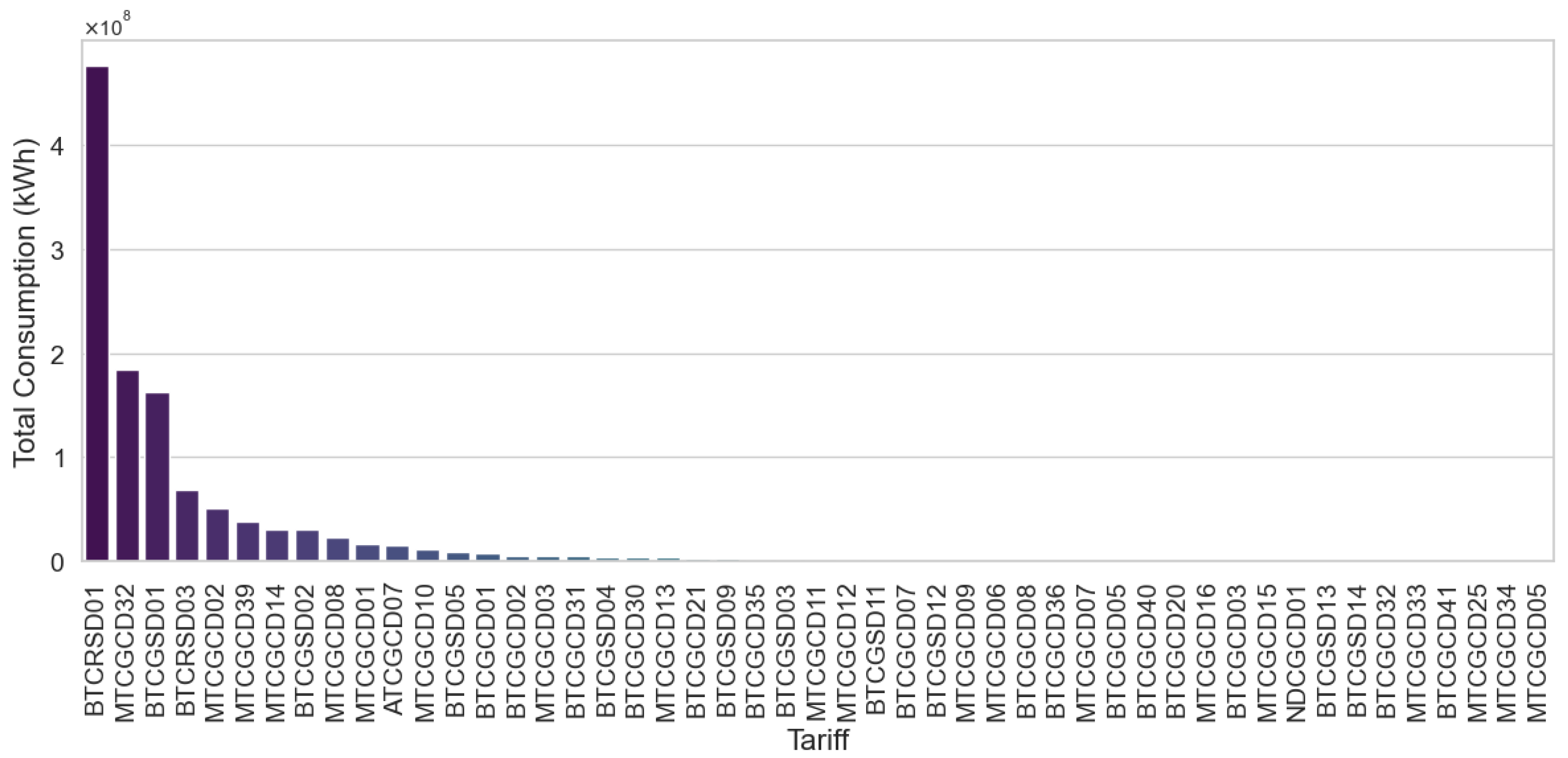
  • Segmentation of the study universe: Based on the analysis of consumption distribution by tariff type (Figure 2), the BTCRSD01 (residential) segment was exclusively selected, given that it contains the highest volume of demanded energy. Consequently, 59,720 records belonging to non-residential clients (19.16% of the total) were excluded. The complete tariff coding is detailed in Table A1.
    Table 2 summarizes the total number of records excluded at each stage of filtering, resulting in a cumulative reduction of 28.95% relative to the original dataset.
    Table 3 in Section 3 details the clean and validated records used for the segmentation of residential tariff consumptions.
  • Normalization of Consumption: In order to homogenize the data scale and prevent magnitude differences from affecting cluster assignment, Z-score normalization was applied to the monthly consumption. This transformation was performed using the following expression:
    X scaled = X μ σ
    where
    -
    X scaled is the normalized data.
    -
    X is the original energy consumption value.
    -
    μ is the mean of the dataset.
    -
    σ is the standard deviation of the dataset.

2.4. Client Segmentation with K-Means

2.4.1. Foundations of the Clustering Algorithm

The segmentation of consumers was conducted utilizing the K-Means algorithm, which is extensively acknowledged in the energy analysis literature for its simplicity, computational efficiency, and capacity to manage substantial volumes of aggregated data [5,7]. The primary aim was to delineate homogeneous groups of residential users based on their monthly consumption patterns, thereby enabling their characterization, the formulation of differentiated tariff schemes, and the identification of atypical consumption behaviors.
The selection of the K-Means algorithm is underpinned by several critical considerations. Primarily, this algorithm is particularly adept at handling extensive databases with limited temporal resolution, exemplified by the monthly billing records analyzed in this study [1,3,4]. K-Means functions by minimizing the aggregate of the squared distances between each data point and the centroid of its cluster, thereby yielding distinct partitions that enhance interpretability and facilitate subsequent applications in both operational and tariff management [1]. The effectiveness of K-Means in analogous contexts has been corroborated by various studies, underscoring its robustness compared to alternative methodologies such as DBSCAN, Fuzzy C-Means, or hierarchical clustering, particularly when the data exhibit low granularity and contain a manageable number of segments to identify [7,8,14].

2.4.2. Criteria for the Determination of the Optimal Number of Clusters

Determining the optimal number of clusters k is a crucial decision in the implementation of the K-Means algorithm, as it significantly affects the quality of segmentation. To address this decision in a rigorous and objective manner, an analytical approach was employed, utilizing the elbow method as a foundation, supplemented by polynomial fitting, which facilitated the smoothing and mathematical derivation of the total inertia curve.
  • Initially, the total inertia, also referred to as the Within-Cluster Sum of Squares (WCSS), was computed across a spectrum of k values, indicating the cumulative squared deviations of each data point from the centroid of its corresponding cluster.
    Inertia = i = 1 n j = 1 k min μ j | | x i μ j | | 2
    where
    -
    n is the total number of data points.
    -
    k is the number of clusters evaluated.
    -
    x i is the i-th data point.
    -
    μ j is the centroid of the j-th cluster.
  • Thereafter, to circumvent decisions reliant on the subjective visual analysis of the WCSS curve, a third-degree polynomial was applied to the inertia values. This facilitated the derivation of a continuous mathematical model indicative of the trend of the curve:
    P ( k ) = a d k d + a d 1 k d 1 + + a 1 k + a 0
    where
    -
    P ( k ) is the polynomial fitted to the inertia values.
    -
    k represents the number of clusters.
    -
    a d , a d 1 , , a 0 are the coefficients of the polynomial.
    -
    d is the degree of the polynomial.
  • Subsequently, the first and second derivatives of the fitted polynomial were evaluated to ascertain the point of maximum curvature, thereby determining the optimal value of k.
    P ( k ) = d P ( k ) d k
    P ( k ) = d 2 P ( k ) d k 2
    where
    -
    P ( k ) represents the first derivative of the fitting polynomial with respect to k.
    -
    P ( k ) represents the second derivative of the polynomial.
  • Finally, the curvature radius formula was applied for each value of k, with the aim of quantifying the local curvature of the smoothed curve and finding the point where it reaches its minimum value:
    R ( k ) = ( 1 + P ( k ) 2 ) 3 2 | P ( k ) |
    where
    -
    R ( k ) is the radius of curvature at each value of k.

2.4.3. Execution of the Clustering Methodology

After establishing the optimal number of clusters, the K-Means algorithm was executed, employing a random initialization of centroids. The iterative method concentrated on minimizing the sum of squared Euclidean distances between the data points and their respective centroids, thereby ensuring convergence towards a stable partitioning.
Each iteration comprises two essential phases:
  • Cluster assignment: Each observation is associated with the nearest centroid using Euclidean distance as the metric.
  • Centroid update: Centroids are recalculated as the average of the points within each cluster.
The algorithm’s objective function, which is intended for minimization, is articulated as follows:
J = j = 1 k x i C j x i μ j 2
where
  • k is the number of defined clusters.
  • x i represents each data point from the set of observations.
  • C j is the set of points assigned to cluster j.
  • μ j is the centroid vector corresponding to cluster j.
  • x i μ j 2 denotes the squared Euclidean distance between x i and μ j .
The centroid is recalibrated at each iteration using the following formalization:
μ j = 1 | C j | x i C j x i
where
  • μ j is the new centroid of cluster j.
  • C j represents the set of points assigned to cluster j.
  • | C j | is the total number of points in cluster j.
This methodology is iteratively executed until the centroids achieve convergence or the predetermined maximum number of iterations is attained. The outcome is a segmentation of users exhibiting uniform consumption patterns, facilitating pricing strategies and enhancing predictive analytics.

2.4.4. Assessment of Clustering Model Efficacy

Following the establishment of the segmentation through K-Means, it is crucial to assess its quality in order to validate the discerned patterns. Accordingly, three complementary metrics were utilized to examine internal cohesion and the separation between clusters.
  • Firstly, the total inertia metric, also known as the WCSS, is employed to evaluate the internal compactness of each cluster. This metric is computed as the aggregate of the squared distances between each data point and its corresponding centroid:
    WCSS = k = 1 K x i C k x i c k 2
    where
    -
    K is the number of clusters.
    -
    C k is the set of points assigned to cluster k.
    -
    x i represents each observation within cluster k.
    -
    c k is the centroid of cluster k.
    -
    x i c k 2 is the squared Euclidean distance between point x i and centroid c k .
  • Secondly, the Silhouette index was utilized, which assesses the similarity degree of each point with its respective cluster in comparison to neighboring clusters. Its value ranges between −1 and +1, with higher values signifying superior separation:
    S ( i ) = b ( i ) a ( i ) max ( a ( i ) , b ( i ) )
    where
    -
    S ( i ) is the Silhouette coefficient for point i.
    -
    a ( i ) is the mean distance between point i and all other points in the same cluster.
    -
    b ( i ) is the mean distance between point i and all points in the nearest cluster to which point i does not belong.
  • Finally, Davies–Bouldin (DB) was used, which quantifies the relationship between the dispersion within the clusters and the separation between them. A lower DB value implies a more defined segmentation:
    D B = 1 k i = 1 k max j i σ i + σ j d ( c i , c j )
    where
    -
    D B is the Davies–Bouldin index.
    -
    k is the number of clusters.
    -
    σ i is the intra-cluster dispersion for cluster i.
    -
    c i and c j are the centroids of clusters i and j, respectively.
    -
    d ( c i , c j ) is the distance between the centroids of clusters i and j.
In summary, these metrics offer an exhaustive assessment of clustering quality, facilitating the identification of the most robust configuration with regard to internal coherence and inter-group separation.

2.5. Practical Implementations of the Segmentation Model

The application of K-Means segmentation to residential consumer data facilitates the identification of homogeneous consumption patterns and enables the implementation of specific applications aimed at improving tariff efficiency, anomaly detection, and demand forecasting. In the subsequent sections, three primary operational applications are elaborated, which are sequentially derived from the clustering outcomes.

2.5.1. Redefinition of Tariffs Based on Consumption Profiles

Based on the centroids of the identified clusters, the consumption ranges for the residential segment were redefined with the aim of designing differentiated pricing schemes that are more representative of the reality of each user group. This approach enables a fairer and more efficient tariff allocation, aligned with the principles of equity and financial sustainability.
  • In the initial phase, the minimum and maximum consumption thresholds for each cluster are determined as follows:
    Min j = min i C j X i
    Max j = max i C j X i
    where
    -
    X i denotes the mean consumption of customer i within cluster C j .
    -
    Min j and Max j signify the lower and upper limits of cluster C j , respectively.
  • Subsequently, to maintain a consistent sequence in the segments, the clusters were systematically reorganized based on the centroid value:
    μ j = 1 | C j | i C j X i
    where
    -
    μ j is the centroid of cluster j.
    -
    | C j | is the number of clients in cluster j.
    -
    Clusters are reordered according to μ j from smallest to largest.
    The new cluster index k is defined as follows:
    k = rank ( μ j )
    where rank ( μ j ) represents the ordered position of the centroid within the set of clusters.

2.5.2. Detection of Anomalous Consumption Through IQR Analysis

Each cluster underwent a distinct evaluation process to identify outliers through the application of the IQR. This methodology facilitated the formulation of thresholds specifically adapted to the intrinsic variability of each cluster, thereby augmenting the detection sensitivity concerning aberrant consumption patterns.
The IQR is delineated as follows:
I Q R = Q 3 Q 1
wherein
  • Q 1 is the first quartile (25th percentile).
  • Q 3 is the third quartile (75th percentile).
The thresholds for the identification of outliers are defined as follows: The lower threshold is defined as follows:
L l o w e r = Q 1 1.5 × I Q R
whereas the upper threshold is defined as follows:
L u p p e r = Q 3 + 1.5 × I Q R
A value X will be considered an outlier if it meets the following condition:
X < L l o w e r or X > L u p p e r

2.5.3. Incorporation of Clustering Techniques Within Demand Forecasting Frameworks

The present study undertakes an evaluation of three complementary predictive methodologies: LR, decision trees (DTs), and RF. In every instance, the cluster label attributed to each customer was utilized as an explanatory categorical variable, in conjunction with parameters such as consumption history, applied rate, and geographical location.
  • LR A foundational multiple LR model was constructed to predict future energy consumption through a linear combination of independent variables:
    Y = β 0 + β 1 X 1 + β 2 X 2 + + β n X n + ε
    where
    -
    Y is the dependent variable (estimated energy consumption).
    -
    X i are the independent variables (factors such as historical consumption, applied tariff, location, etc.).
    -
    β i are the regression coefficients, which indicate the influence of each variable X i .
    -
    β 0 is the Y-intercept (value of Y when X i = 0 ).
    -
    ε is the error or residual term.
  • Decision Tree (DT)
    The decision tree method develops a hierarchical framework of rules systematically partitioning data into homogeneous subsets, employing measures such as entropy or information gain. A primary advantage of this approach is its capacity to model non-linear relationships, alongside its interpretability.
    y ^ = arg max i j = 1 n w j ( y j = i )
    where
    -
    y ^ is the predicted class.
    -
    w j is the weight of observation j.
    -
    ( y j = i ) is an indicator function that is 1 if y j = i and 0 otherwise.
    Nonetheless, singular DTs are prone to overfitting when confronted with noisy data, which subsequently impacts their generalization capability.
  • RF To address the issue of overfitting, the RF methodology was implemented. This approach synthesizes multiple DTs, each trained on randomly selected subsets of data and variables. Consequently, the model enhances the stability of predictions and effectively diminishes variance:
    P ( y | X ) = 1 T t = 1 T f t ( X )
    where
    -
    P ( y | X ) is the probability that instance X belongs to class y.
    -
    T is the total number of trees in the RF.
    -
    f t ( X ) is the prediction of tree t.
The evaluation of the model’s performance was executed using established metrics, namely Mean Absolute Error (MAE), Root Mean Squared Error (RMSE), and the Coefficient of Determination ( R 2 ).
  • Mean Absolute Error (MAE):
    M A E = 1 n i = 1 n | Y i Y ^ i |
    where
    -
    Y i is the actual energy consumption value.
    -
    Y ^ i is the value predicted by the model.
    -
    n is the total number of observations.
    Lower MAE values indicate better model accuracy.
  • Root Mean Squared Error (RMSE):
    R M S E = 1 n i = 1 n ( Y i Y ^ i ) 2
    where
    -
    Y i is the actual value.
    -
    Y ^ i is the predicted value.
    -
    n is the number of observations.
    A low RMSE value indicates a model with more precise predictions and fewer extreme errors.
  • The Coefficient of Determination ( R 2 ):
    R 2 = 1 i = 1 n ( Y i Y ^ i ) 2 i = 1 n ( Y i Y ¯ ) 2
    where
    -
    Y ¯ is the mean of the actual values.
    -
    Y i are the actual values.
    -
    Y ^ i are the predicted values.
    An R 2 close to 1 indicates a model with high predictive power, while values close to 0 suggest that the model does not explain the variability of the data well.

3. Results

3.1. Descriptive Analysis of the Examined Data

The analysis utilized a dataset comprising 221,401 validated records pertaining to residential customers categorized under the rate BTCRSD01, encompassing the period from January 2023 to December 2024. The preprocessing phase incorporated the elimination of inactive accounts, as well as records exhibiting null or negative consumption and inconsistencies, thereby ensuring a representative sample of active users characterized by authentic consumption patterns.
The variables under consideration comprise the registration date, the contractual identifier, the geographical location, and the monthly consumption measured in kWh. Table 3 provides a summary of their typology and cardinality.
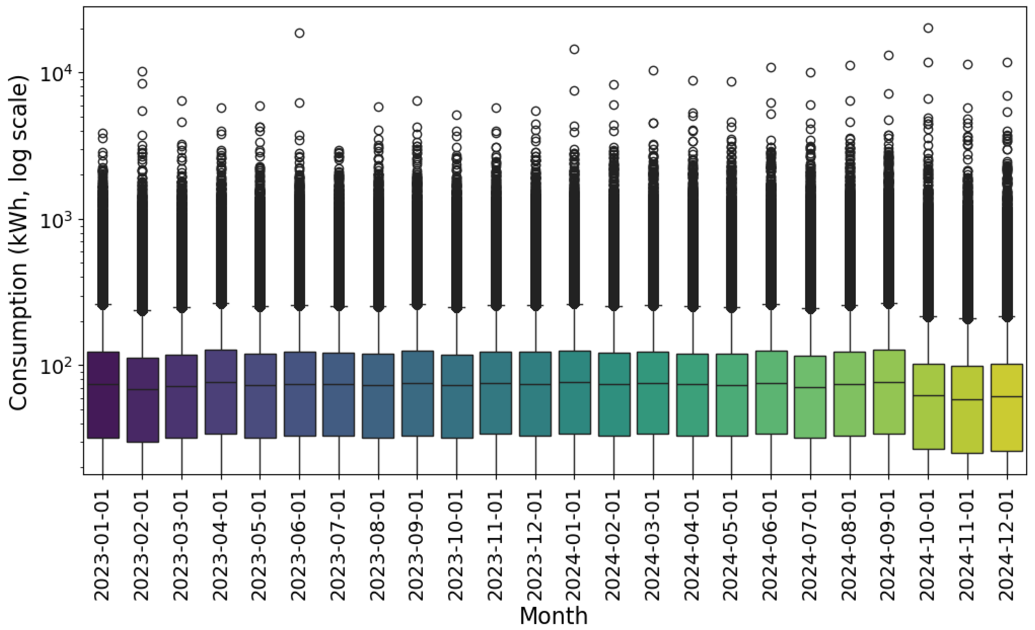
Figure 3 illustrates the distribution of monthly consumption on a logarithmic scale. There is significant heterogeneity among users, characterized by a notable concentration in the range of low to medium consumption (approximately 100 kWh/month) and a persistent occurrence of outliers. This variability substantiates the utilization of segmentation techniques to facilitate more efficient and precise rate management.

3.2. Determining and Validating the Optimal Quantity of Clusters

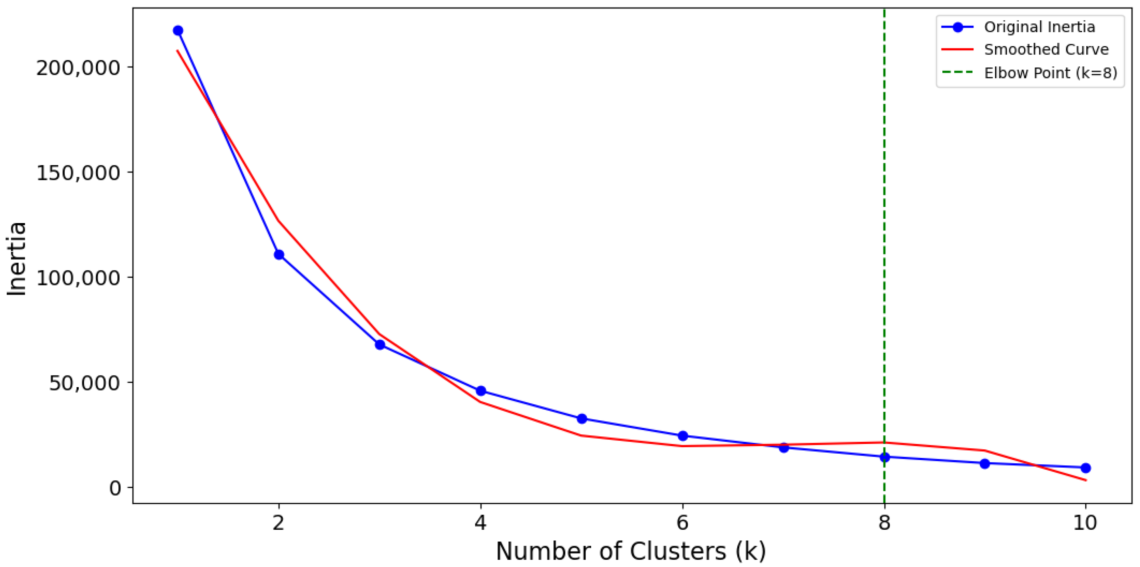
The determination of the optimal number of clusters was conducted by utilizing the elbow method on the WCSS, employing a third-degree polynomial fit to smooth the curve. Subsequently, the second derivative facilitated the precise identification of the point of maximum curvature, as illustrated in Figure 4.
The comprehensive evaluation of these criteria revealed that the optimal number of clusters is k = 8, as this configuration achieves a suitable equilibrium between internal compactness and intergroup separation, thereby mitigating the risks of both overfitting and underfitting.
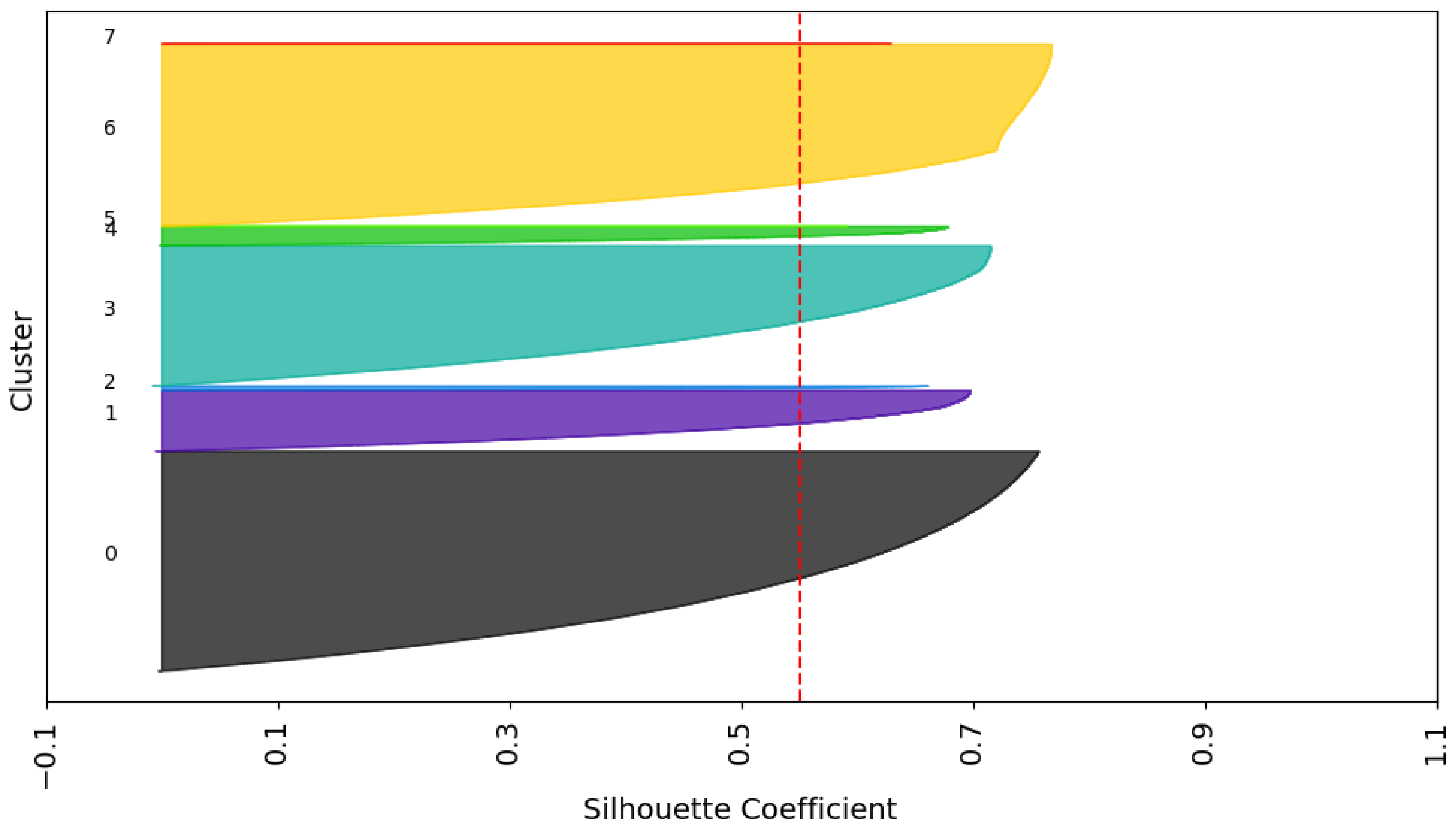
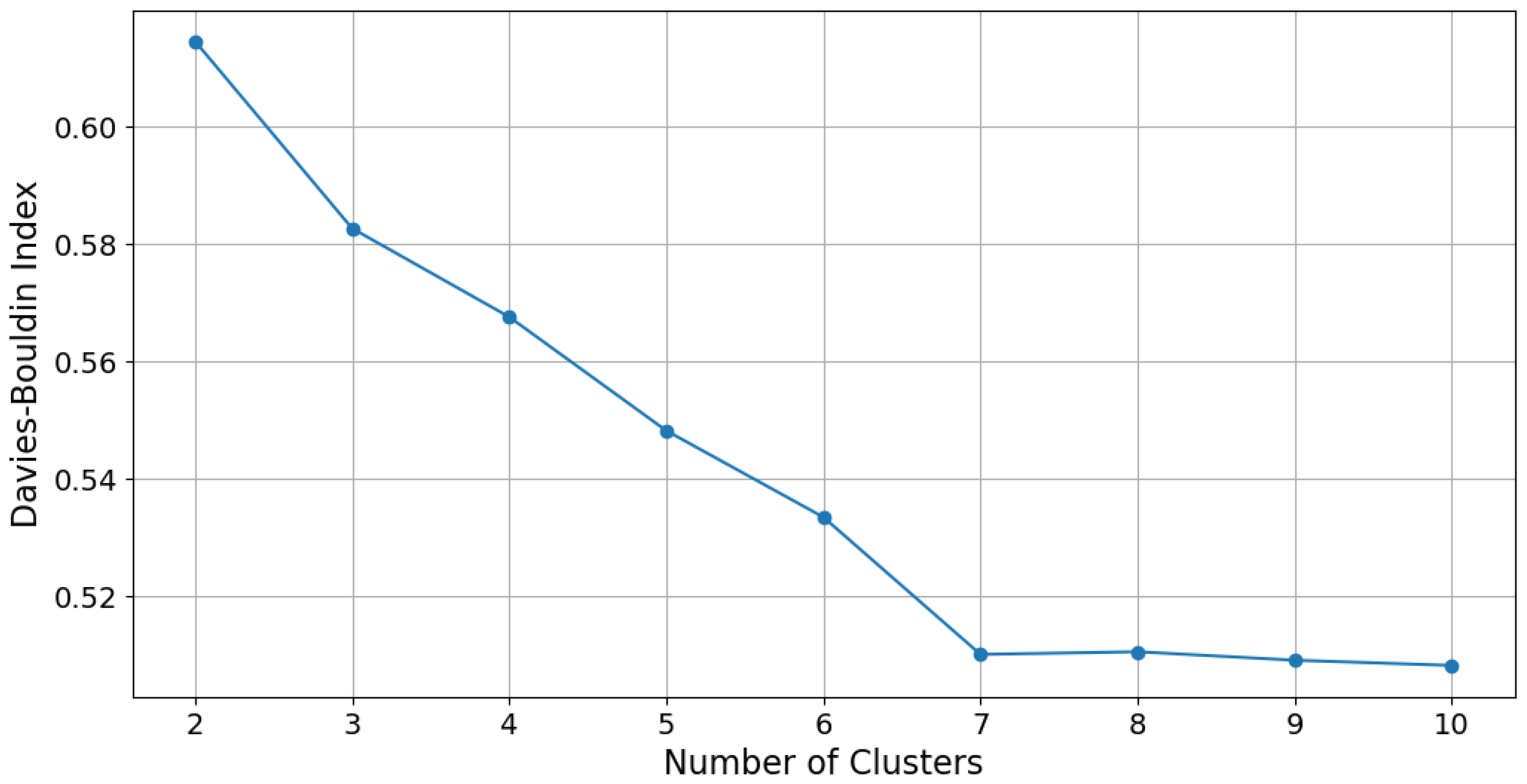
Table 4 presents a summary of the validation metrics for the models under evaluation. The silhouette score (0.55) alongside the minimum Davies–Bouldin index (0.51) corroborates the robustness of the segmentation achieved.
The analysis was further augmented by the assessment of the Silhouette and Davies–Bouldin indices, as depicted in Figure 5 and Figure 6.

3.3. Examination of the Identified Clusters

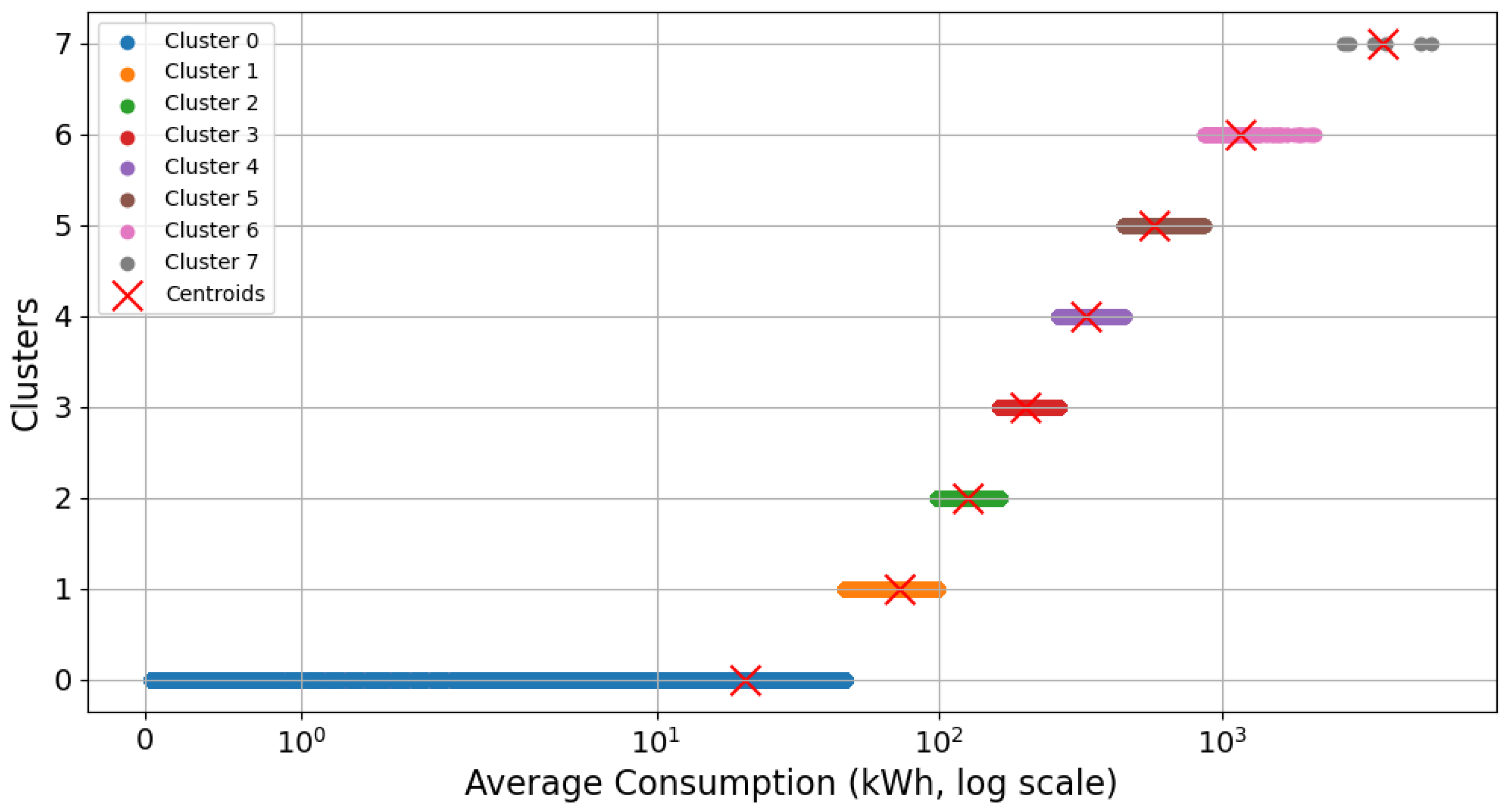
Upon ascertaining that the optimal number of clusters was k = 8, the K-Means clustering algorithm was employed to classify residential users subscribing to the BTCRSD01 tariff. Table 5 illustrates the centroids of each cluster, which epitomize the typical monthly consumption levels, extending from users with very low electricity usage (approximately 21 kWh/month) to those categorized as large residential consumers (exceeding 3700 kWh/month).
Figure 7 depicts the distribution of users according to their allocated cluster, thereby demonstrating a distinct separation between the groups and underscoring the efficacy of the segmentation process.
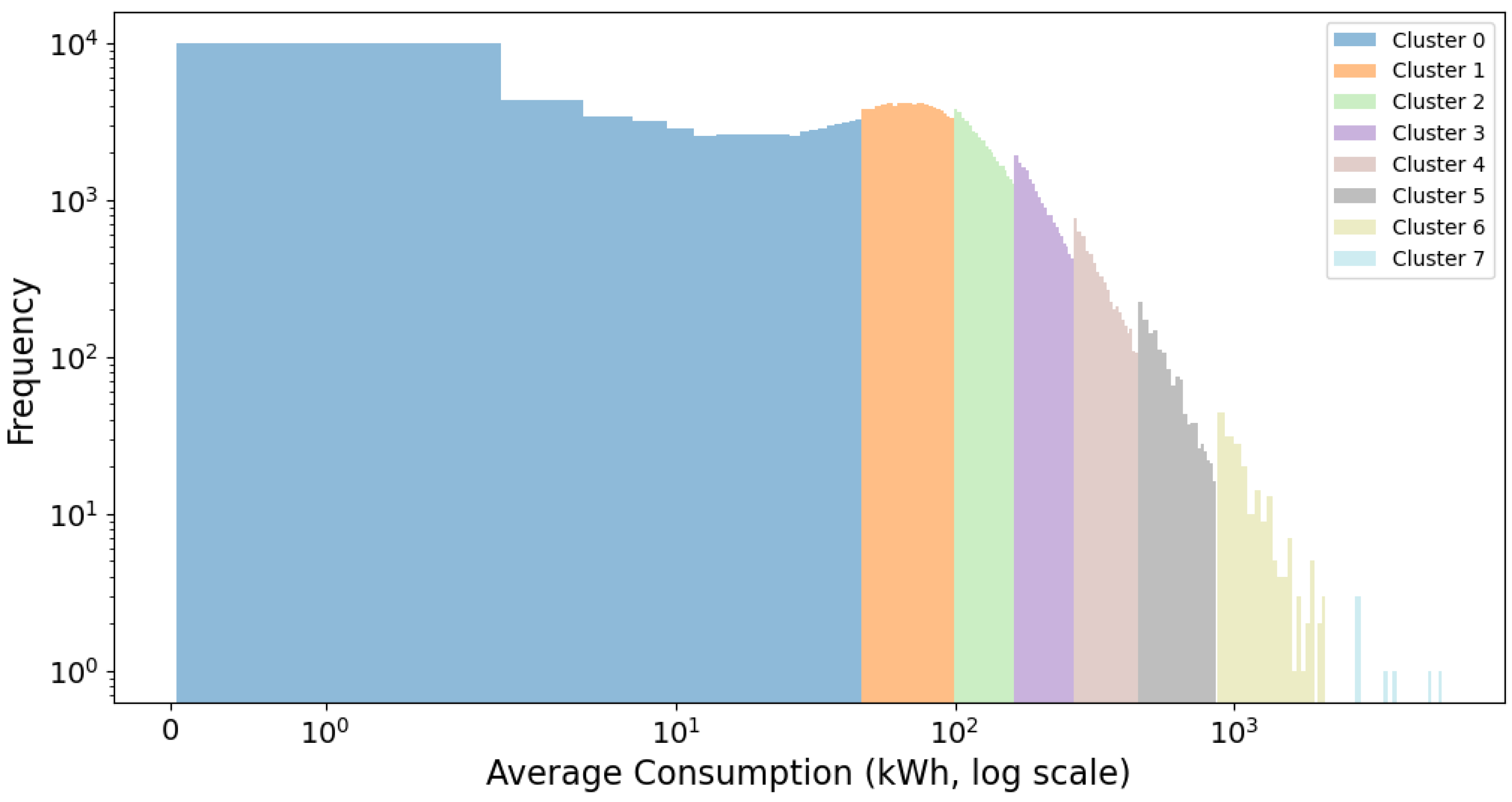
As depicted in Figure 8, it is evident that the majority of customers are categorized into clusters of low and medium consumption, whereas the clusters associated with high consumption exhibit a substantially smaller quantity of users.
For the distribution enterprise, this segmentation constitutes an essential instrument for managerial operations. It facilitates the customization of energy efficiency initiatives by cluster, directs investments toward infrastructure, and predicts consumption trends based on profile, thereby enhancing the optimization of network planning and resource allocation. Table A2 elucidates the optimal number of clusters identified for alternative rates, thereby enabling the methodology’s application across diverse tariff segments.

3.4. A Comparative Analysis of Existing and Suggested Rates

Following an analysis of the centroids derived from K-Means segmentation, new consumption ranges for the residential rate labeled BTCRSD01 have been proposed. The objective is to align the rate brackets with the actual usage patterns identified. This reformulation not only simplifies the tariff structure but also enhances its economic efficiency and reinforces regulatory coherence.
Table 6 delineates the newly defined intervals based on the lower and upper boundaries of each of the eight identified clusters. These segments encompass a consumption range extending from 1 to in excess of 5500 kWh per month. It is noteworthy that over 93% of users are predominantly situated within the initial six levels, indicating a significant density within the low and medium consumption categories. This concentration facilitates the formation of tiered rate structures without compromising the consistency of revenue collection.
Conversely, Table 7 illustrates the ranges currently enacted by EEASA, which are distinguished by a more subdivided segmentation into 15 segments determined by arbitrary thresholds, such as multiples of 50 or 100 kWh. This configuration fails to accurately capture the true diversity of consumption patterns, potentially leading to distortions in the economic signals perceived by users and fostering tariff inequities.
The proposed approach through clustering offers three key advantages:
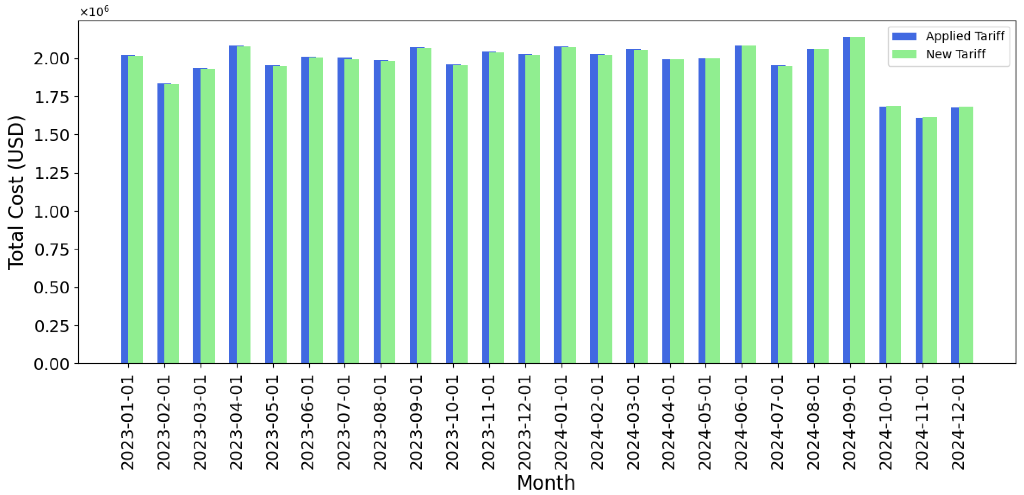
  • Economic Efficiency: The revised tariff structures are designed to more precisely reflect consumption patterns, thereby enhancing the precision in the allocation of tariff charges and mitigating economic distortions. In addition, as shown in Figure 9, the preservation of total system revenue guarantees the financial stability of the distributor.
  • Regulatory Viability: By ensuring that the tariff structure adheres to the boundaries set forth by the national regulatory framework while maintaining anticipated revenue streams, the proposal is technically feasible and can be executed without compromising the operational sustainability of the company.
  • Tariff Equity: The categorization of users based on analogous consumption patterns into distinct blocks fortifies the principle of distributive justice. Furthermore, this approach diminishes the number of users situated near pivotal thresholds, consequently reducing incentives for arbitrage and enhancing the perception of transparency within the tariff framework.
In conclusion, clustering-based segmentation facilitates the development of a pricing structure that is more representative, efficient, and equitable, without adversely affecting the distributor’s revenue or necessitating intricate alterations to the measurement infrastructure. These results underscore the potential of unsupervised learning as a strategic instrument for tariff redesign in contexts lacking smart metering capabilities.
Table A3 delineates the specific details of tailored consumption ranges pertinent to various rates, thereby illustrating the adaptability of the methodology across diverse segments.

3.5. Outcomes of Anomaly Identification by Cluster

To detect atypical consumption behaviors, the IQR method was employed within each of the eight clusters delineated via the K-Means algorithm. This approach facilitated the establishment of bespoke thresholds attuned to the statistical variability inherent in each group, thereby augmenting the precision in outlier identification without necessitating advanced measurement techniques.
The examination of Cluster 1, encompassing the largest cohort of residential customers (71,844 users), has disclosed notable deviations from the group’s average consumption patterns. Instances of exceptionally low consumption were identified, which may be attributable to vacant properties or interruptions in supply. Conversely, instances of excessively high consumption were also observed, potentially indicative of non-residential activities, billing inaccuracies, or unauthorized connections.
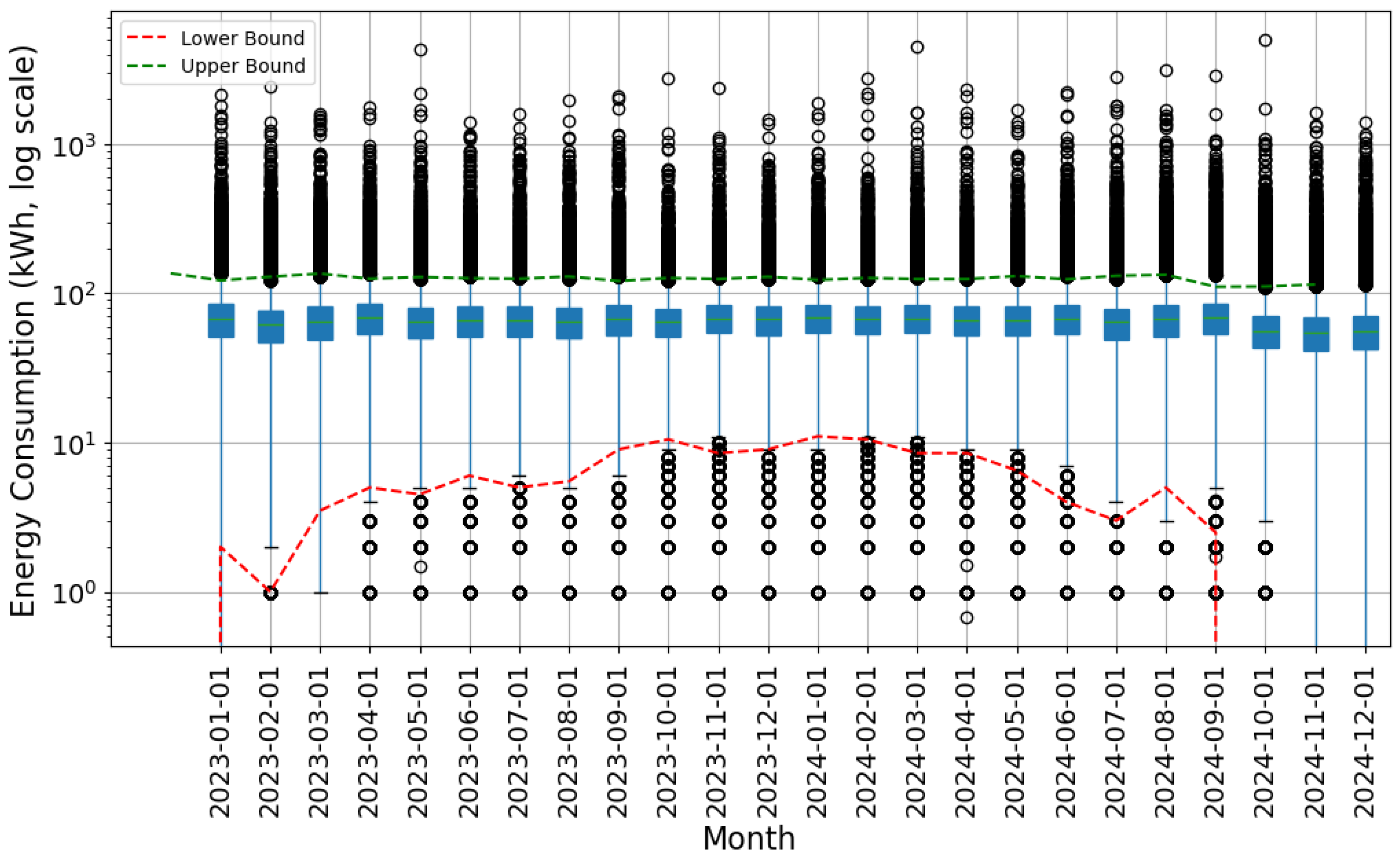
Figure 10 delineates the specified detection thresholds for this cluster, providing a graphical representation of the anticipated normal consumption range, thereby aiding operational analysis. The use of the IQR at the cluster level enables a more accurate differentiation compared to global approaches, taking into account the structural diversity within the user population.
Table 8 provides a monthly summary of detected outlier cases. On average, 1176 users exhibited consumption levels below the expected threshold (0.53%), while 1973 users demonstrated values exceeding this threshold (0.89%). Notably, the months of February and May 2023 exhibited significant spikes in anomalies, indicating the potential influence of seasonal patterns or specific events that merit further detailed examination.
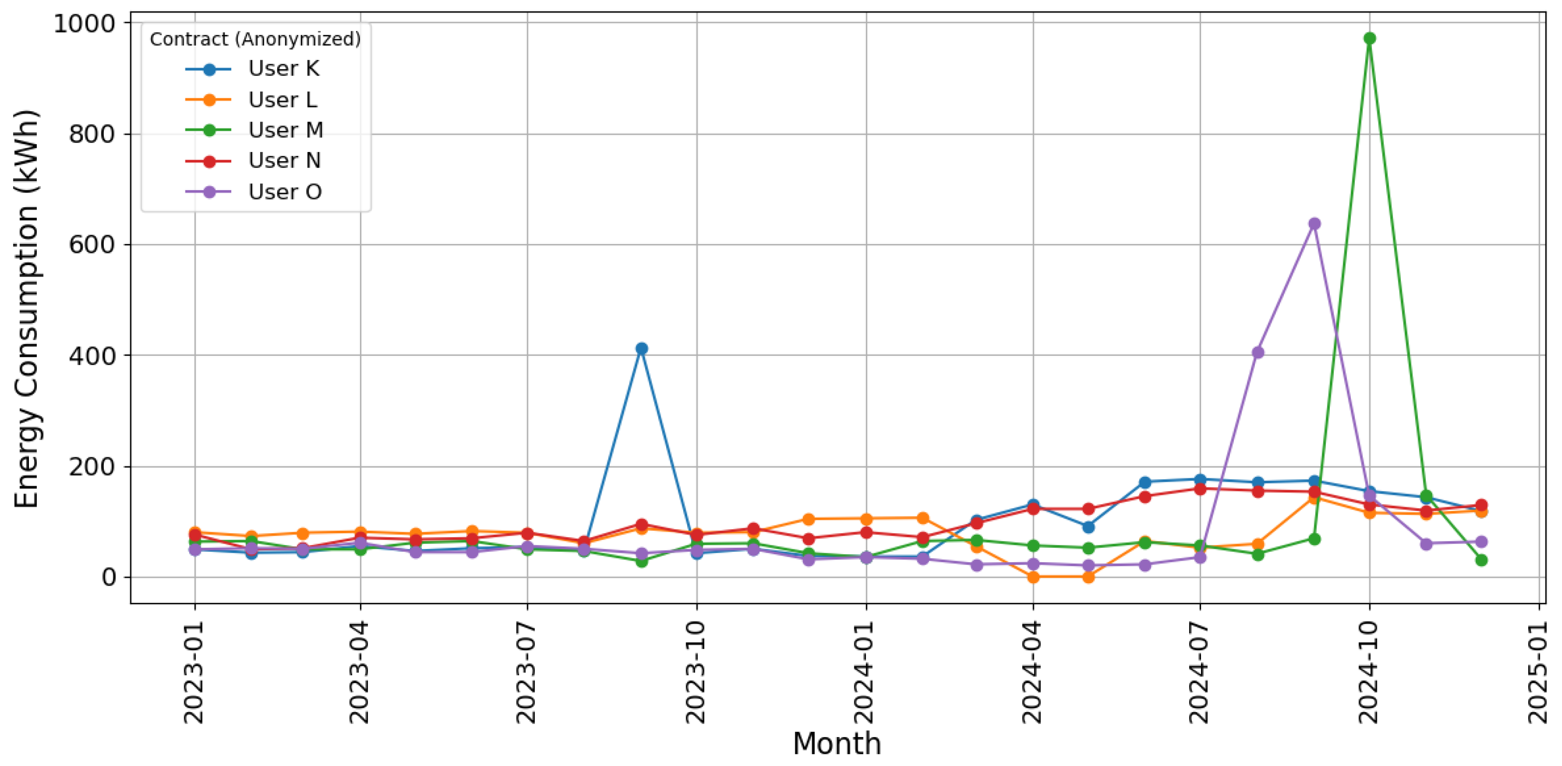
Figure 11 and Figure 12 illustrate instances of lower and upper outliers, respectively. The former could be associated with unoccupied properties, measurement inaccuracies, or unrecorded disconnections. Conversely, the latter might suggest misuse of the residential rate, errors, or fraudulent activity.
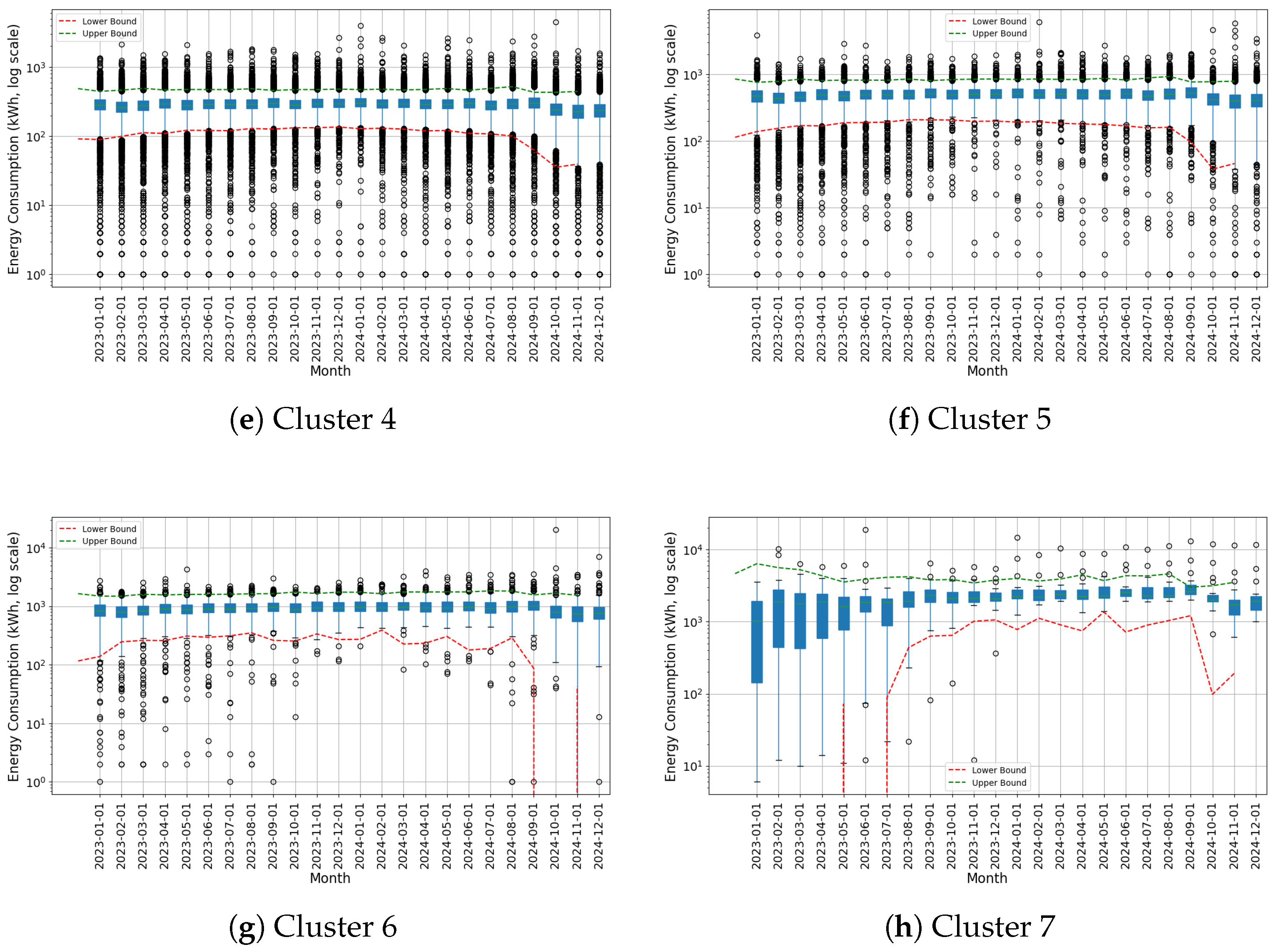
From an operational standpoint, the methodology predicated on clustering and the IQR enables distribution companies to prioritize inspections, allocate resources to critical cases, and formulate automated alerts to mitigate non-technical losses. This capability for early detection is especially beneficial in contexts devoid of smart metering infrastructure. Figure A1 elucidates the application of this analysis for the eight clusters delineated within the residential rate.

3.6. Assessment of the Efficacy of Predictive Models

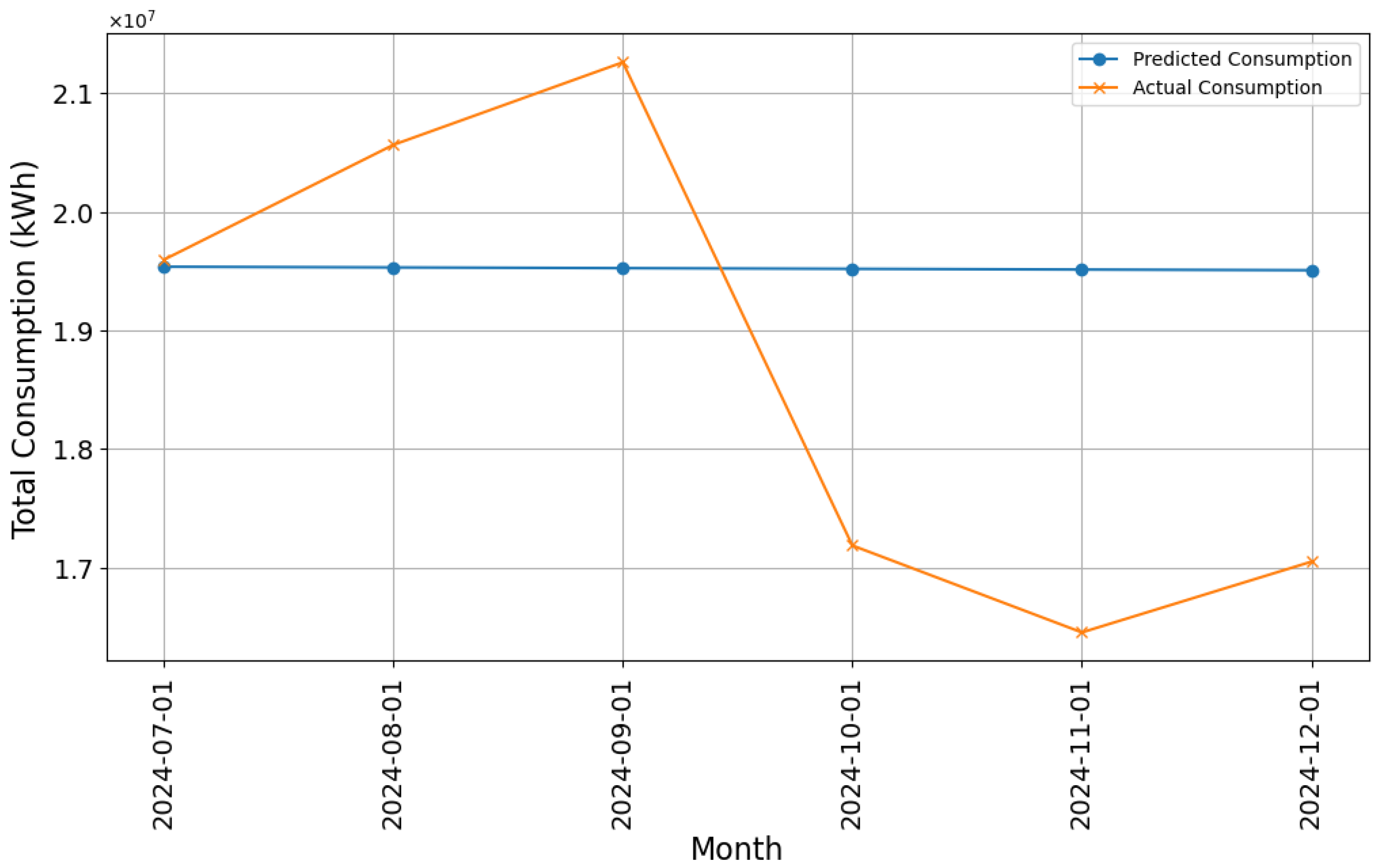
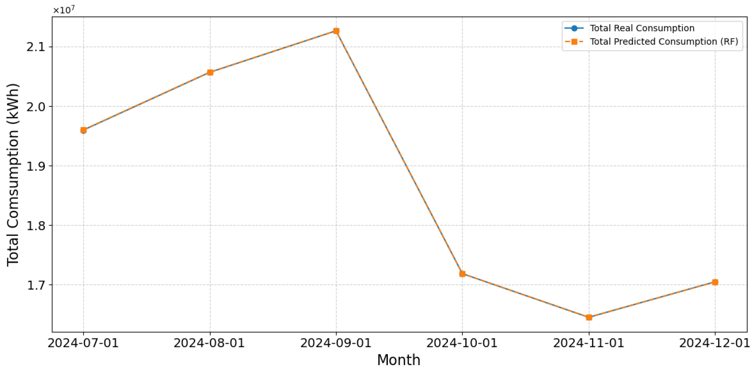
To assess the predictive capability of the segmentation model, three methodologies were evaluated: LR, DTs, and RF, each employing the cluster label as an explanatory variable. Table 9 presents a summary of the results obtained from the evaluation. The LR model exhibited suboptimal performance, evidenced by a coefficient of determination R2 of merely 0.12, highlighting its inadequacy in capturing the variability inherent in consumption patterns. Conversely, models grounded in ML methodologies demonstrated notable enhancements: the decision tree model achieved an R2 of 0.56, and the RF model attained an R2 of 0.67, indicating superior capacities for generalization and fitting.
Figure 13 demonstrates the projection produced by the LR model, which inaccurately estimates demand across various periods, thereby constraining its operational effectiveness.
Conversely, Figure 14 illustrates the projection of the RF model, which demonstrates a heightened ability to forecast consumption peaks and troughs with greater precision, thereby exhibiting superior adaptation to the historical patterns observed.
From the perspective of the distributor, the accuracy of models is critical for planning energy procurement, preventing grid overloads, and making well-informed strategic decisions in data-limited environments. The findings indicate that incorporating the cluster as a predictive variable substantially improves the estimation of energy demand.

4. Discussion

4.1. Assessment of Segmentation Model and Performance

The application of the K-Means algorithm facilitated the effective segmentation of residential consumers into homogeneous groups, which exhibited distinct patterns of energy consumption. The determination of the optimal cluster count was executed using the elbow method and further substantiated by the Silhouette and Davies–Bouldin indices, whose values demonstrated a distinct separation among groups and appropriate internal cohesion. These findings align with those articulated by Wu (2024), who employed an optimized variant of K-Means (IHHO-K-Means) in the evaluation of electric consumers in southern China, achieving efficacious and differentiated groupings [8].
Mahdi (2023) asserts that K-Means continues to be an effective and computationally economical method for systems lacking smart measurement infrastructure, as exemplified by the current study [7]. Furthermore, the utilization of a monthly data structure conforms to the guidelines proposed by Rajabi (2017), who underscores the practicality of clustering within contexts characterized by low temporal granularity [5].

4.2. Comparison with Previous Studies

The conclusions of this study are consistent with a range of international research conducted in comparable contexts. Umar (2019) utilized clustering methodologies to categorize customers and identify non-technical losses within Nigerian electrical systems [6]. Similarly, in this analysis, an analogous method is adopted wherein outliers are regarded as significant deviations warranting preliminary examination, without necessarily indicating fraud or anomaly.
Henriques (2024) employed ML techniques in Brazil to model residential consumption patterns. Utilizing billing data analogous to those of the present study, the research substantiates that average curves derived from clustering provide a precise representation of the aggregate demand [1]. In addition, Rathod (2017) advocates for the implementation of clustering to formulate more efficient pricing strategies, a method that underscores the potential of this study for segmented pricing. This perspective is further supported by Ofetotse (2021), who analyze determinants of consumption in Botswana and recommend the utilization of segmentations for the development of progressive tariff policies [2,4].
Ultimately, the study conducted by AbuBaker (2019) reveals that the application of data mining in the electrical sector can significantly enhance the understanding of customer behavior and support strategic decisions through clustering, highlighting the value of this analysis as an essential planning tool [3].

4.3. Practical Applications: Tariff Formulation, Planning, and Early Detection of Anomalous Consumption

The applicability of segmentation is articulated within three principal dimensions:
Segmented pricing: The grouping of customers based on their energy behavior allows for the design of differentiated tariffs that reflect the actual use of energy, promoting pricing efficiency and equity, as indicated in the studies by Wu (2024) and Rathod (2017) [4,8].
Early identification of atypical consumption: Clients exhibiting consumption patterns markedly divergent from the mean of their respective cluster have been identified, which may indicate billing inaccuracies, fraudulent activities, or anomalous circumstances. Such preliminary detection permits timely technical or commercial evaluations, consistent with the frameworks proposed by Umar (2019) and AbuBaker (2019) [3,6].
Projection of demand in the absence of smart metering: The creation of standard curves, organized by clusters and derived from normalized consumption data, assists in the simulation and planning of demand. This approach replicates the successful methodologies documented by Ofetotse (2021) and Rajabi (2017) [2,5].

4.4. Limitations of This Study

A prominent constraint of this study is the limited temporal resolution of the data, recorded on a monthly basis, which hinders the ability to capture intraday or weekly dynamics. Furthermore, the lack of socioeconomic, climatic, or cadastral variables restricts the scope of multivariable analysis pertaining to consumer behavior.
Rajabi (2017) and Ofetotse (2021) emphasize that a more comprehensive segmentation approach necessitates the inclusion of supplementary attributes, including income level, geographic location, household size, and type of equipment. Furthermore, this study lacks field cross-validation, requiring that the identified profiles and outliers undergo verification in future phases [2,5].

4.5. Potential Avenues for Enhancement and Future Lines of Inquiry

The current study initiates multiple trajectories of applied research. Notably, it advocates for the integration of dynamic clustering algorithms, including online K-Means and Hidden Markov Models, to effectively capture the temporal dynamics of consumption patterns. Furthermore, it is proposed to investigate hybrid models that amalgamate clustering with supervised algorithms, such as DTs and neural networks, for the purposes of classifying new clients or projecting their prospective demand, as indicated in Wu (2024) and Mahdi (2023) [7,8].
From an operational standpoint, the amalgamation of climatic, topological, and socioeconomic data facilitates the development of more resilient, flexible, and utilitarian models for tariff formulation and energy strategic planning in environments characterized by minimal technological infrastructure.
The findings derived from this study corroborate that segmentation based on the K-Means algorithm serves as an efficacious, consistent, and cost-efficient methodology for optimizing tariff and operational governance in networks lacking smart metering, despite the presence of data constraints.

5. Conclusions

5.1. Validation of the Hypothesis and Methodological Contributions

The findings of this research corroborate the posited hypothesis: employing the K-Means algorithm on monthly electric billing records proficiently segments residential customers. This is achieved even in the absence of smart metering, thereby yielding valuable insights for pricing strategies, demand forecasting, and the identification of anomalous behaviors.
From a methodological perspective, it has been empirically established that preprocessing by means of Z-score normalization, coupled with the meticulous determination of the optimal number of clusters, guarantees robust and replicable outcomes. This rigor is critical for its implementation in distribution electrical systems lacking smart meters.

5.2. Practical Applications for System Planning and Operation

A significant contribution of this study is its applicability in designing differentiated pricing structures tailored to the actual consumption behaviors of consumers. This segmentation of tariffs may enhance distributive equity and facilitate a more efficient allocation of subsidies.
The model’s capability for the early detection of outliers has been substantiated, facilitating the prioritization of technical or commercial inspections during the preliminary phases. This early warning capacity is critical for mitigating non-technical losses in systems characterized by constrained resources, particularly in areas with traditional infrastructure.
Conversely, the potential to allocate type load curves to customers in the absence of advanced metering serves as a valuable basis for enhancing demand estimation methodologies, refining operational planning, and optimizing load flow simulations within distribution networks.

5.3. Restrictions and Recommendations for Future Research

A prominent limitation of this study is the limited temporal granularity of the dataset utilized, which impedes the comprehensive analysis of nuanced intraday or seasonal fluctuations. Additionally, the absence of integration with sociodemographic or geospatial variables constrains the explanatory capacity of the model.
For future research endeavors, it is advisable to investigate dynamic clustering algorithms, such as adaptive K-Means and online clustering, along with hybrid methodologies that amalgamate supervised classification with unsupervised segmentation to facilitate the automatic allocation of new users into representative clusters. Furthermore, it is proposed to integrate climatic, social, and economic variables to augment multivariable segmentation and improve its applicability in sophisticated pricing frameworks.

5.4. Principal Contributions of This Research

  • Effective Segmentation Without Smart Metering: The model proficiently classified consumers exhibiting uniform consumption behaviors by solely employing monthly billing data.
  • Optimization of the Tariff Structure: The reclassification of consumption categories utilizing cluster centroids enhances equity, mitigates economic distortions, and maintains financial sustainability.
  • The IQR method effectively facilitated the early detection of anomalous consumption by accurately identifying outliers, thus allowing for prioritized inspections without requiring the installation of smart meters.
  • Enhanced Predictive Modeling: By incorporating the cluster as a covariate, the RF model attained an R 2 of 0.67, in contrast to 0.12 obtained with LR.
  • Practical Applicability and Replicability: The strategy proposed herein is cost-effective, replicable, and adaptable to a wide range of utilities operating within environments where data are limited.

Author Contributions

Conceptualization, D.M.-M.; methodology, D.M.-M. and M.A.-C.; software, D.M.-M.; validation, D.M.-M. and M.A.-C.; formal analysis, D.M.-M. and M.A.-C.; investigation, D.M.-M.; resources, D.M.-M.; data curation, D.M.-M.; writing—original draft preparation, D.M.-M.; writing—review and editing, D.M.-M.; visualization, D.M.-M.; supervision, M.A.-C.; project administration, M.A.-C.; funding acquisition, M.A.-C. All authors have read and agreed to the published version of the manuscript.

Funding

This research received no external funding.

Data Availability Statement

The original contributions presented in this study are included in the article. Further inquiries can be directed to the corresponding author.

Acknowledgments

The authors would like to express their gratitude to Universidad Indoamérica for its support of this research through the “Tecnologías de la Industria 4.0 en Educación, Salud, Empresa e Industria” project.

Conflicts of Interest

The authors declare no conflicts of interest.

Abbreviations

The following abbreviations are used in this manuscript:
EEASAEmpresa Eléctrica Ambato Regional Centro Norte S.A.
IQRInterquartile Range
WCSSWithin-Cluster Sum of Squares
MLMachine Learning
LRLinear Regression
DTsDecision Trees
RFRandom Forest

Appendix A. Tariff Classification and Description

Table A1. Tariff codes and descriptions.
No.CodeName
1BTCGSD03(BT/Social Assistance)
2BTCGCD03(BT/Social Assistance with Demand)
3NDCGCD01(BT/Social Assistance with Hourly Demand)
4BTCGSD04(BT/Public Benefit)
5BTCGCD05(BT/Public Benefit with Demand)
6BTCGCD20(BT/Public Benefit with Hourly Demand)
7BTCGCD21(BT/Water Pumping for Rural Communities)
8BTCGSD14(BT/Water Pumping for Public Water Service)
9BTCGCD40(BT/Water Pumping for Public Water Service with Hourly Demand)
10BTCGSD01(BT/Commercial)
11BTCGCD01(BT/Commercial with Demand)
12BTCGCD31(BT/Commercial with Hourly Demand)
13BTCGSD09(BT/Religious Worship)
14BTCGCD32(BT/Religious Worship with Demand)
15BTCGSD05(BT/Official Entities)
16BTCGCD07(BT/Official Entities with Demand)
17BTCGCD35(BT/Official Entities with Hourly Demand)
18BTCGCD08(BT/Sports Venues with Demand)
19BTCGSD02(BT/Artisan Industrial)
20BTCGCD02(BT/Industrial with Demand)
21BTCGCD30(BT/Industrial with Hourly Demand)
22BTCGSD12(BT/Sports Venues)
23BTCGSD13(BT/Water Pumping)
24BTCGSD11(BT/Community Service)
25BTCGCD36(BT/Sports Venues with Hourly Demand)
26BTCRSD01(BT/Residential)
27BTCGCD41(BT/Electric Vehicles with Hourly Demand)
28MTCGCD05(MT/Special Subscribers with Demand)
29MTCGCD06(MT/Special Subscribers with Hourly Demand)
30MTCGCD07(MT/Social Assistance with Demand)
31MTCGCD08(MT/Social Assistance with Hourly Demand)
32MTCGCD09(MT/Public Benefit with Demand)
33MTCGCD10(MT/Public Benefit with Hourly Demand)
34MTCGCD11(MT/Water Pumping with Demand)
35MTCGCD12(MT/Water Pumping with Hourly Demand)
36MTCGCD01(MT/Commercial with Demand)
37MTCGCD02(MT/Commercial with Hourly Demand)
38MTCGCD13(MT/Official Entities with Demand)
39MTCGCD14(MT/Official Entities with Hourly Demand)
40MTCGCD15(MT/Sports Venues with Demand)
41MTCGCD16(MT/Sports Venues with Hourly Demand)
42MTCGCD25(MT/Fast Charging Station with Differentiated Hourly Demand)
43MTCGCD03(MT/Industrial with Demand)
44MTCGCD32(MT/Industrial with Differentiated Hourly Demand)
45MTCGCD34(MT/Community Service with Hourly Demand)
46MTCGCD39(MT/Water Pumping for Public Water Service with Hourly Demand)
47ATCGCD07(AT/Industrial with Differentiated Hourly Demand)
48BTCRSD03(BT/Residential for PEC Program)
49MTCGCD33(MT/Religious Worship with Demand)
BT, MT, and AT denote user connection levels: BT (Low Voltage), MT (Medium Voltage), and AT (High Voltage), used for tariff classification and grid planning.

Appendix B. Cluster Analysis Results

Table A2. Optimal clusters and centroids by tariff code.
Tariff CodeOptimal ClustersCentroids
NDCGCD012[2394.43, 2895.9]
MTCGCD062[5331.01, 9263.33]
BTCGCD402[2399.95, 7418.65]
BTCGCD202[2270.96, 5712.8]
BTCGCD322[419.4, 2560.62]
BTCGCD033[1543.6, 891.0, 2642.58]
BTCGCD413[80.62, 159.79, 201.42]
BTCGCD084[171.36, 5632.1, 7048.62, 556.2]
BTCGCD054[1931.63, 497.42, 2946.97, 1616.7]
MTCGCD074[408.89, 1821.18, 3609.1, 1173.09]
MTCGCD334[129.41, 326.92, 31.54, 299.28]
MTCGCD145[3181.5, 37,063.96, 78,734.7, 129,109.17, 15,625.5]
MTCGCD135[282.56, 11,677.47, 4070.26, 1853.76, 6591.21]
MTCGCD105[2153.27, 165,376.34, 49,857.05, 19,763.66, 5138.79]
BTCGSD135[198.63, 18.91, 1066.88, 385.58, 101.52]
MTCGCD095[522.69, 3124.49, 1842.01, 164.14, 1058.21]
MTCGCD035[349.85, 2668.15, 10,839.59, 1183.11, 5242.4]
MTCGCD015[247.49, 4149.28, 2454.36, 6417.11, 1243.05]
BTCGSD145[812.89, 12.5, 300.06, 1085.94, 673.54]
MTCGCD325[45,893.64, 1,358,196.0, 4329.7, 506,672.25, 163,288.16]
MTCGCD395[5047.56, 531,873.08, 83,837.75, 335,595.17, 39,288.78]
BTCGCD015[999.16, 4328.42, 6442.52, 13,346.06, 2500.26]
BTCGCD355[3427.68, 25,806.39, 7436.79, 1253.66, 9800.71]
BTCGCD025[2110.8, 1040.54, 3546.75, 8462.81, 439.58]
BTCGCD215[158.81, 26,779.32, 6890.7, 12,042.01, 1453.09]
BTCGCD305[3198.38, 7522.15, 17,195.32, 1241.18, 5261.49]
BTCGCD365[5618.13, 496.87, 4970.8, 883.61, 139.4]
BTCGSD125[26.25, 1429.3, 409.18, 721.21, 148.47]
MTCGCD126[2546.22, 17,676.27, 73.74, 8817.99, 16,204.77, 1479.83]
MTCGCD167[89.25, 1639.05, 694.62, 2024.52, 1470.12, 181.94, 655.86]
MTCGCD157[54.83, 3990.0, 467.93, 119.28, 194.78, 429.54, 117.38]
BTCGSD058[628.38, 2094.26, 42.97, 4716.99, 3422.08, 1201.18, 7659.57, 255.87]
BTCGSD048[13.85, 832.42, 186.8, 1797.49, 331.17, 527.47, 1217.01, 85.32]
BTCRSD018[20.63, 72.25, 125.39, 201.52, 328.42, 573.09, 1159.36, 3725.24]
BTCGSD038[34.28, 782.41, 2350.22, 333.84, 1577.29, 552.38, 1231.3, 160.32]
BTCGCD079[188.97, 3001.96, 5893.12, 1624.22, 1172.06, 3559.69, 2167.13, 724.29, 398.31]

Appendix C. Consumption Range Analysis Results

Table A3. Consumption ranges per tariff.
Tariff CodeConsumption Ranges
BTCGCD01[0, 1687, 3329, 5100, 8620, 14,381, superior]
BTCGCD02[0, 721, 1527, 2742, 5484, 8462, superior]
BTCGCD03[0, 890, 1694, 2642, superior]
BTCGCD05[0, 517, 1616, 1978, 3053, superior]
BTCGCD07[0, 259, 443, 723, 1173, 1706, 2176, 3062, 3563, 5892, superior]
BTCGCD08[0, 171, 555, 5631, 7048, superior]
BTCGCD20[0, 2500, 5712, superior]
BTCGCD21[0, 613, 2631, 8808, 12748, 29,007, superior]
BTCGCD30[0, 2176, 4222, 6186, 8521, 17,194, superior]
BTCGCD31[0, 1149, 2354, 3613, 5425, 7375, 9080, 12,649, 23,056, superior]
BTCGCD32[0, 487, 2560, superior]
BTCGCD35[0, 1822, 4518, 7568, 9800, 25,805, superior]
BTCGCD36[0, 138, 496, 965, 4970, 5617, superior]
BTCGCD40[0, 2596, 7418, superior]
BTCGCD41[0, 80, 159, 200, superior]
BTCGSD01[0, 126, 305, 551, 899, 1409, 2137, 3306, 6785, superior]
BTCGSD02[0, 111, 238, 412, 669, 1042, 1542, 2328, 3699, superior]
BTCGSD03[0, 95, 242, 412, 655, 959, 1347, 1576, 2723, superior]
BTCGSD04[0, 48, 134, 257, 423, 677, 998, 1457, 2245, superior]
BTCGSD05[0, 148, 439, 904, 1612, 2693, 3865, 4978, 7659, superior]
BTCGSD09[0, 79, 219, 439, 800, 1064, 1407, 1684, 2673, superior]
BTCGSD11[0, 57, 164, 322, 507, 848, 1288, 1497, 2031, superior]
BTCGSD12[0, 85, 255, 530, 930, 1717, superior]
BTCGSD13[0, 56, 138, 216, 456, 1066, superior]
BTCGSD14[0, 31, 308, 673, 826, 1113, superior]
BTCRSD01[0, 45, 98, 162, 264, 450, 863, 2119, 5520, superior]
BTCRSD03[0, 53, 101, 151, 213, 302, 445, 731, 1523, superior]
NDCGCD01[0, 2393, 2895, superior]
MTCGCD01[0, 739, 1844, 3222, 5157, 8161, superior]
MTCGCD02[0, 3399, 8148, 14,958, 22,692, 33,649, 44,426, 75,424, 277,851, superior]
MTCGCD03[0, 756, 1895, 3562, 5471, 14,583, superior]
MTCGCD06[0, 5330, 9262, superior]
MTCGCD07[0, 429, 1359, 2068, 3608, superior]
MTCGCD08[0, 6001, 15,648, 32,224, 46,589, 104,668, 147,726, 170,948, 222,813, superior]
MTCGCD09[0, 299, 631, 1175, 2184, 3789, superior]
MTCGCD10[0, 3634, 6700, 23,791, 64,368, 165,375, superior]
MTCGCD11[0, 93, 280, 630, 1058, 1543, 2348, 4211, 18,810, superior]
MTCGCD12[0, 146, 1479, 2545, 8817, 16,204, 17,675, superior]
MTCGCD13[0, 1021, 2821, 5141, 7273, 12,383, superior]
MTCGCD14[0, 9139, 25,234, 46,236, 78,734, 129,108, superior]
MTCGCD15[0, 54, 116, 119, 194, 429, 467, 3989, superior]
MTCGCD16[0, 93, 181, 655, 694, 1469, 1638, 2024, superior]
MTCGCD32[0, 24,461, 86,416, 252,215, 610,251, 1,358,195, superior]
MTCGCD33[0, 31, 128, 298, 326, superior]
MTCGCD39[0, 21489, 55,492, 100,345, 335,594, 531,872, superior]

Appendix D. Cluster Analysis Results for Residential Tariff
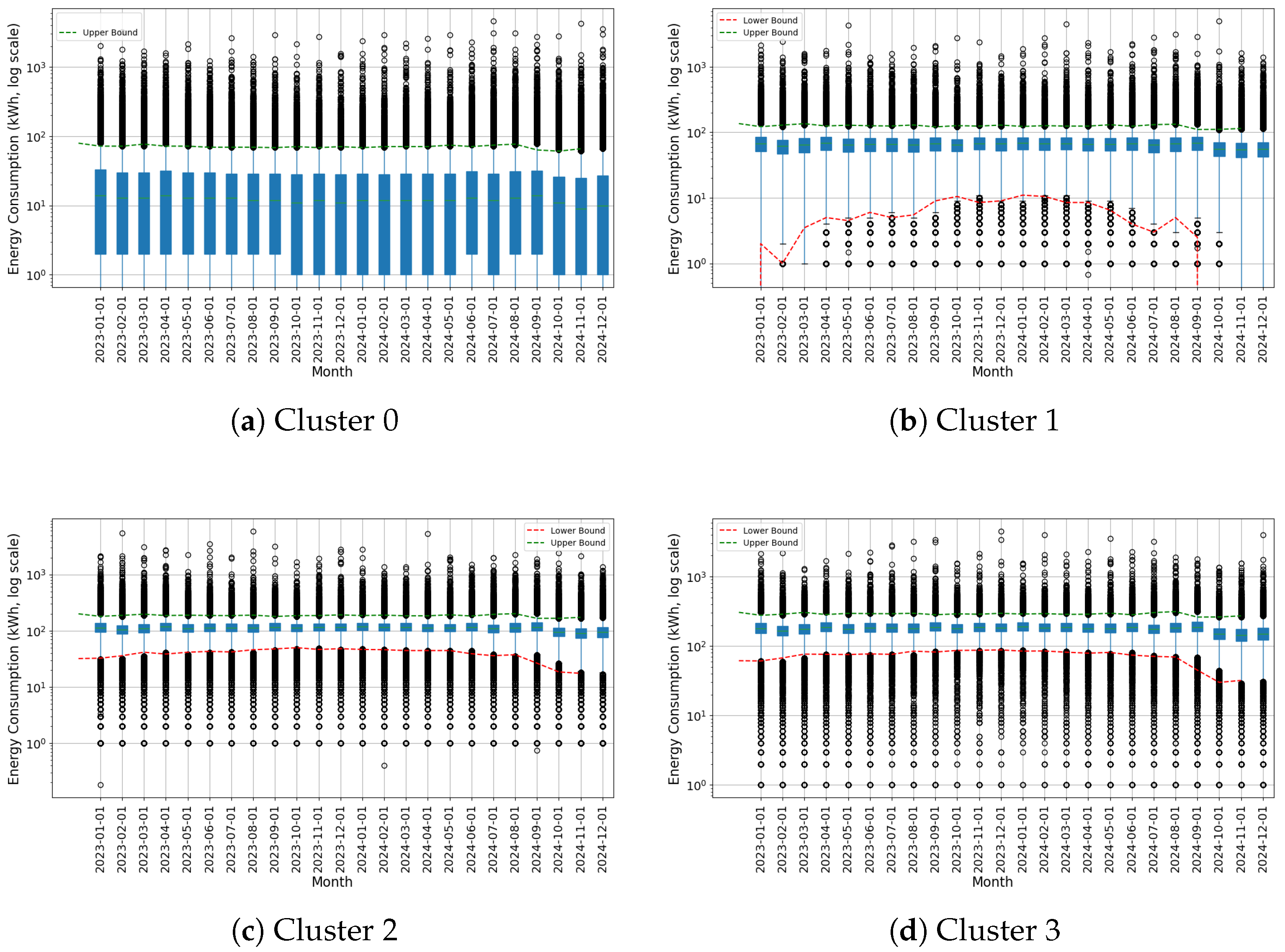
Figure A1. Outlier detection per cluster and month based on residential electricity consumption patterns. Black circles depict the consumption values attributed to individual users. Blue columns illustrate the cluster’s monthly median consumption. The red and green dotted lines denote the lower and upper bounds, respectively, as determined by the Interquartile Range (IQR) method.
Energies 18 03083 g0a1aEnergies 18 03083 g0a1b

References

  1. Henriques, L.; Lima, F.; Castro, C. Combining Advanced Feature-Selection Methods to Uncover Atypical Energy-Consumption Patterns. Future Internet 2024, 16, 229. [Google Scholar] [CrossRef]
  2. Ofetotse, E.; Essah, E.; Yao, R. Evaluating the determinants of household electricity consumption using cluster analysis. J. Build. Eng. 2021, 43, 102487. [Google Scholar] [CrossRef]
  3. AbuBaker, M. Data mining applications in understanding electricity consumers’ behavior: A case study of Tulkarm district, Palestine. Energies 2019, 12, 4287. [Google Scholar] [CrossRef]
  4. Rathod, R.; Garg, R. Design of electricity tariff plans using gap statistic for K-means clustering based on consumers monthly electricity consumption data. Int. J. Energy Sect. Manag. 2017, 11, 295–310. [Google Scholar] [CrossRef]
  5. Rajabi, A.; Li, L.; Zhang, J.; Zhu, J.; Ghavidel, S.; Ghadi, M. A review on clustering of residential electricity customers and its applications. In Proceedings of the 2017 20th International Conference on Electrical Machines and Systems, ICEMS 2017, Sydney, Australia, 11–14 August 2017. [Google Scholar] [CrossRef]
  6. Umar, H.; Prasad, R.; Fonkam, M. Assessing severity of non-technical losses in power using clustering Algorithms. In Proceedings of the 2019 15th International Conference on Electronics, Computer and Computation, ICECCO 2019, Abuja, Nigeria, 10–12 December 2019. [Google Scholar] [CrossRef]
  7. Miraftabzadeh, S.; Colombo, C.; Longo, M.; Foiadelli, F. K-Means and Alternative Clustering Methods in Modern Power Systems. IEEE Access 2023, 11, 119596–119633. [Google Scholar] [CrossRef]
  8. Wu, R. Behavioral analysis of electricity consumption characteristics for customer groups using the k-means algorithm. Syst. Soft Comput. 2024, 6, 200143. [Google Scholar] [CrossRef]
  9. Amri, Y.; Fadhilah, A.; Fatmawati; Setiani, N.; Rani, S. Analysis Clustering of Electricity Usage Profile Using K-Means Algorithm. In Proceedings of the IOP Conference Series: Materials Science and Engineering, Yogyakarta, Indonesia, 11–12 November 2015; Volume 105. [Google Scholar] [CrossRef]
  10. Kwac, J.; Flora, J.; Rajagopal, R. Lifestyle Segmentation Based on Energy Consumption Data. IEEE Trans. Smart Grid 2018, 9, 2409–2418. [Google Scholar] [CrossRef]
  11. Sarmas, E.; Fragkiadaki, A.; Marinakis, V. Explainable AI-Based Ensemble Clustering for Load Profiling and Demand Response. Energies 2024, 17, 5559. [Google Scholar] [CrossRef]
  12. Michalakopoulos, V.; Sarmas, E.; Papias, I.; Skaloumpakas, P.; Marinakis, V.; Doukas, H. A machine learning-based framework for clustering residential electricity load profiles to enhance demand response programs. Appl. Energy 2024, 361, 122943. [Google Scholar] [CrossRef]
  13. Kaur, R.; Gabrijelčič, D. Behavior segmentation of electricity consumption patterns: A cluster analytical approach. Knowl.-Based Syst. 2022, 251, 109236. [Google Scholar] [CrossRef]
  14. Fernandes, M.; Viegas, J.; Vieira, S.; Sousa, J. Segmentation of residential gas consumers using clustering analysis. Energies 2017, 10, 2047. [Google Scholar] [CrossRef]
  15. Toussaint, W.; Moodley, D. Clustering Residential Electricity Consumption Data to Create Archetypes that Capture Household Behaviour in South Africa. S. Afr. Comput. J. 2020, 32, 1–34. [Google Scholar] [CrossRef]
  16. Wang, S.; Song, A.; Qian, Y. Predicting Smart Cities’ Electricity Demands Using K-Means Clustering Algorithm in Smart Grid. Comput. Sci. Inf. Syst. 2023, 20, 657–678. [Google Scholar] [CrossRef]
  17. Albayati, A.; Abdullah, N.; Abu-Samah, A.; Mutlag, A.; Nordin, R. Smart grid data management in a heterogeneous environment with a hybrid load forecasting model. Appl. Sci. 2021, 11, 9600. [Google Scholar] [CrossRef]
Figure 1. Illustration of the general methodological framework employed in this research.
Energies 18 03083 g001
Figure 2. Aggregate energy consumption categorized by tariff.
Energies 18 03083 g002
Figure 3. Monthly consumption distribution—residential tariff. Each color is indicative of a specific month, spanning from January 2023 to December 2024.
Energies 18 03083 g003
Figure 4. The elbow method in the context of residential tariffs.
Energies 18 03083 g004
Figure 5. The silhouette plot corresponding to the eight clusters within the tariff residential dataset. Each color represents a different cluster identified by the K-Means algorithm. The red dotted line indicates the average silhouette coefficient across all clusters.
Energies 18 03083 g005
Figure 6. Davies–Bouldin index–number of clusters—residential tariff.
Energies 18 03083 g006
Figure 7. Cluster distribution of residential customers based on average monthly consumption (log scale).
Energies 18 03083 g007
Figure 8. Frequency distribution of residential consumption by cluster (log scale).
Energies 18 03083 g008
Figure 9. Monthly comparison of total residential tariff collection: applied vs. proposed tariff structure.
Energies 18 03083 g009
Figure 10. Monthly anomaly detection bounds for residential Cluster 1 (log-scaled energy consumption. Black circles represent the individual consumption values for each user. Blue columns indicate the monthly median consumption of the cluster. The red and green dotted lines correspond to the lower and upper bounds, respectively, computed using the IQR method.
Energies 18 03083 g010
Figure 11. Time series of representative lower outliers in residential electricity consumption.
Energies 18 03083 g011
Figure 12. Time series of representative upper outliers in residential electricity consumption.
Energies 18 03083 g012
Figure 13. Predicted vs. actual energy consumption using LR—residential tariff.
Energies 18 03083 g013
Figure 14. Predicted vs. actual energy consumption using RF—residential tariff.
Energies 18 03083 g014
Table 1. Exposition of the variables examined in this study.
VariableDescriptionData TypeCardinality
dateConsumption record dateDate24
contract accountUnique identifier for the customer’s contractNumeric311,625
geographic locationParish where the customer is locatedCategorical125
applied tariffType of tariff applied to the customerCategorical54
energy consumptionElectrical energy consumption in kWhNumeric-
Cardinality represents the number of distinct values each variable can take.
Table 2. Overview of the data cleaning and debugging procedure.
StageRecords RemovedPercentage of Total (%)
Inactive Accounts (zero consumption)21,5266.91
Outliers (negative consumption)89782.88
Non-residential Segments59,72019.16
Total Filtered Records90,22428.95
Table 3. Variable descriptions for residential tariffs.
VariableDescriptionData TypeCardinality
dateConsumption record dateDate24
contract accountUnique identifier for the customer’s contractNumeric221,401
geographic locationParish where the customer is locatedCategorical99
energy consumptionElectrical energy consumption in kWhNumeric-
Cardinality represents the number of distinct values each variable can take.
Table 4. Metrics for validating clustering models.
ModelWCSSSilhouetteDavies–Bouldin
K-Means (k = 8)20,0000.550.51
Table 5. Results of consumption segmentation for the residential tariff.
TariffOptimal ClustersCluster Centroids [kWh]
Residential8[20.63, 72.25, 125.39, 201.52, 328.42, 573.09, 1159.36, 3725.24]
Table 6. Proposed tariff structure based on segmented residential consumption.
TariffRangeMin Consumption (kWh)Max Consumption (kWh)Tariff Charge (USD/kWh)Average Customers
BTCRSD0110.00.0013,300
21.045.00.090057,760
346.098.00.092071,844
499.0162.00.095044,913
5163.0264.00.097620,606
6265.0450.00.10276958
7451.0863.00.12851841
8864.02119.00.1709287
92120.05520.00.436018
105521.0Superior0.68120
Table 7. Official tariff structure for residential customers used by EEASA without consumption segmentation.
TariffRangeMin Consumption (kWh)Max Consumption (kWh)Tariff Charge (USD/kWh)Average Customers
BTCRSD01100013,000
20500.091077,753
3511000.093067,410
41011500.095037,385
51512000.097016,658
62012500.09907842
72513000.10103992
83013500.10302195
93515000.10502714
105017000.12851010
1170110000.1450378
12100115000.1709142
13150125000.275244
14250135000.43608
153501Superior0.68120
Table 8. Monthly count of lower and upper outliers for residential consumption—Cluster 1.
ClusterMonthLower OutliersUpper Outliers
11 January 202302544
11 February 202314852513
11 March 202310242292
11 April 202314482339
11 May 202315232278
11 June 202314042096
11 July 202313502109
11 August 202311892016
11 September 202311531808
11 October 202313011688
11 November 202313491513
11 December 202311431523
11 January 202411321374
11 February 202413081607
11 March 202413661639
11 April 202414691753
11 May 202415231636
11 June 202413471766
11 July 202413941915
11 August 202412612074
11 September 202415402281
11 October 202415362208
11 November 202402088
11 December 202402227
Table 9. Comparative results of ML models for energy consumption prediction.
ModelMAERMSER2
LR6.308.50.12
DTs25.3067.120.56
RF25.2058.410.67
Disclaimer/Publisher’s Note: The statements, opinions and data contained in all publications are solely those of the individual author(s) and contributor(s) and not of MDPI and/or the editor(s). MDPI and/or the editor(s) disclaim responsibility for any injury to people or property resulting from any ideas, methods, instructions or products referred to in the content.