
Segmentation of Energy Consumption Using K-Means: Applications in Tariffing, Outlier Detection, and Demand Prediction in Non-Smart Metering Systems


Abstract
1. Introduction
1.1. Significance of Energy Consumption Forecasting in Networks Lacking Smart Metering Systems
1.2. State of the Art in Clustering Techniques and Consumption Profiling
1.3. Main Applications of Clustering in Contexts Without the Presence of Smart Meters
- Tariff Segmentation. Numerous studies have utilized K-Means to classify residential consumers based on consumption patterns derived from monthly or low-frequency records. This segmentation facilitates the definition of tariff profiles that more accurately reflect the user’s reality, enhancing equity and reducing economic distortions. AbuBaker (2019) applied K-Means to prepaid billing data in Palestine, successfully establishing consumption profiles with direct implications for tariff policies [3]. Henriques (2024) additionally demonstrates that a structured segmentation facilitates the allocation of differentiated fees and enhances users’ perception of equity [1].
- Detection of fraud and non-technical losses. Another significant application is the identification of atypical consumption within each homogeneous group. The combined use of K-Means and statistical methods such as the IQR has facilitated the detection of potential fraud, measurement errors, or non-technical losses, even in the absence of hourly information. Umar (2019) integrated K-Means and DBSCAN to identify non-technical losses in Nigeria, demonstrating their operational efficacy in the absence of smart meters [6]. Similarly, Ofetotse (2021) employed household survey data from Botswana and validated its segmentation using Silhouette and Davies–Bouldin indices, thus demonstrating their applicability in contexts with informational constraints [2].
- Energy Demand Prediction. Ultimately, the integration of cluster variables into prediction models has been shown to enhance both the explanatory power and the accuracy of algorithms, especially those based on machine learning (ML). Wang (2023) demonstrated that the incorporation of segmentation using K-Means significantly improves the accuracy of urban electricity demand prediction models [16]. Albayati (2021) also concludes that the integration of clustering methods with RF algorithms surpasses the typical limitations associated with LR, particularly in contexts characterized by incomplete or disaggregated data [17].
1.4. Objective of This Study and Research Hypothesis
2. Materials and Methods
2.1. Overall Structure of the Methodology
2.2. Origin and Description of Consumption Data
- Data from the customer: contract account code and user identifiers.
- Energy consumption: monthly history of electrical consumption expressed in kWh.
- Billing: breakdown of monetary charges associated with recorded consumption.
- Subsidies: information on economic benefits applied to the user.
- Administrative and geographical data: the parish location of the customer and tariff category.
2.3. Data Preprocessing
- Cleaning of inactive records: In total, 21,526 accounts with no recorded consumption during the 2023–2024 period were removed, equivalent to 6.91% of the total. This stage allowed for the analysis to focus exclusively on active users, ensuring the statistical validity of the extracted consumption patterns.
- Removal of inconsistencies due to negative values: In total, 8978 records with negative consumption values (2.88% of the total) were identified and discarded, considered atypical or erroneous due to potential measurement, entry, or re-billing errors.
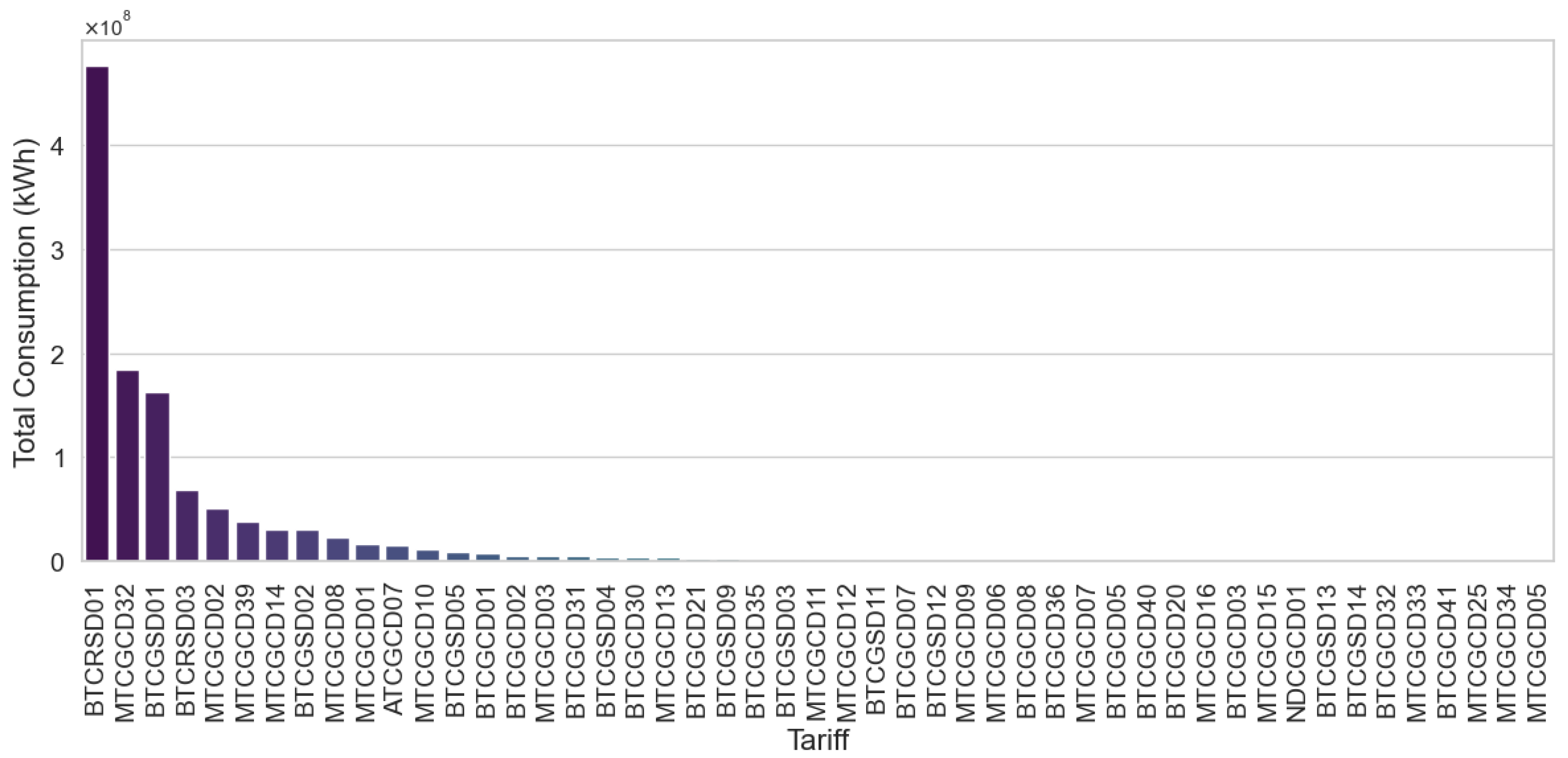
- Segmentation of the study universe: Based on the analysis of consumption distribution by tariff type (Figure 2), the BTCRSD01 (residential) segment was exclusively selected, given that it contains the highest volume of demanded energy. Consequently, 59,720 records belonging to non-residential clients (19.16% of the total) were excluded. The complete tariff coding is detailed in Table A1.Table 2 summarizes the total number of records excluded at each stage of filtering, resulting in a cumulative reduction of 28.95% relative to the original dataset.
- Normalization of Consumption: In order to homogenize the data scale and prevent magnitude differences from affecting cluster assignment, Z-score normalization was applied to the monthly consumption. This transformation was performed using the following expression:where
- -
- is the normalized data.
- -
- X is the original energy consumption value.
- -
- is the mean of the dataset.
- -
- is the standard deviation of the dataset.
2.4. Client Segmentation with K-Means
2.4.1. Foundations of the Clustering Algorithm
2.4.2. Criteria for the Determination of the Optimal Number of Clusters
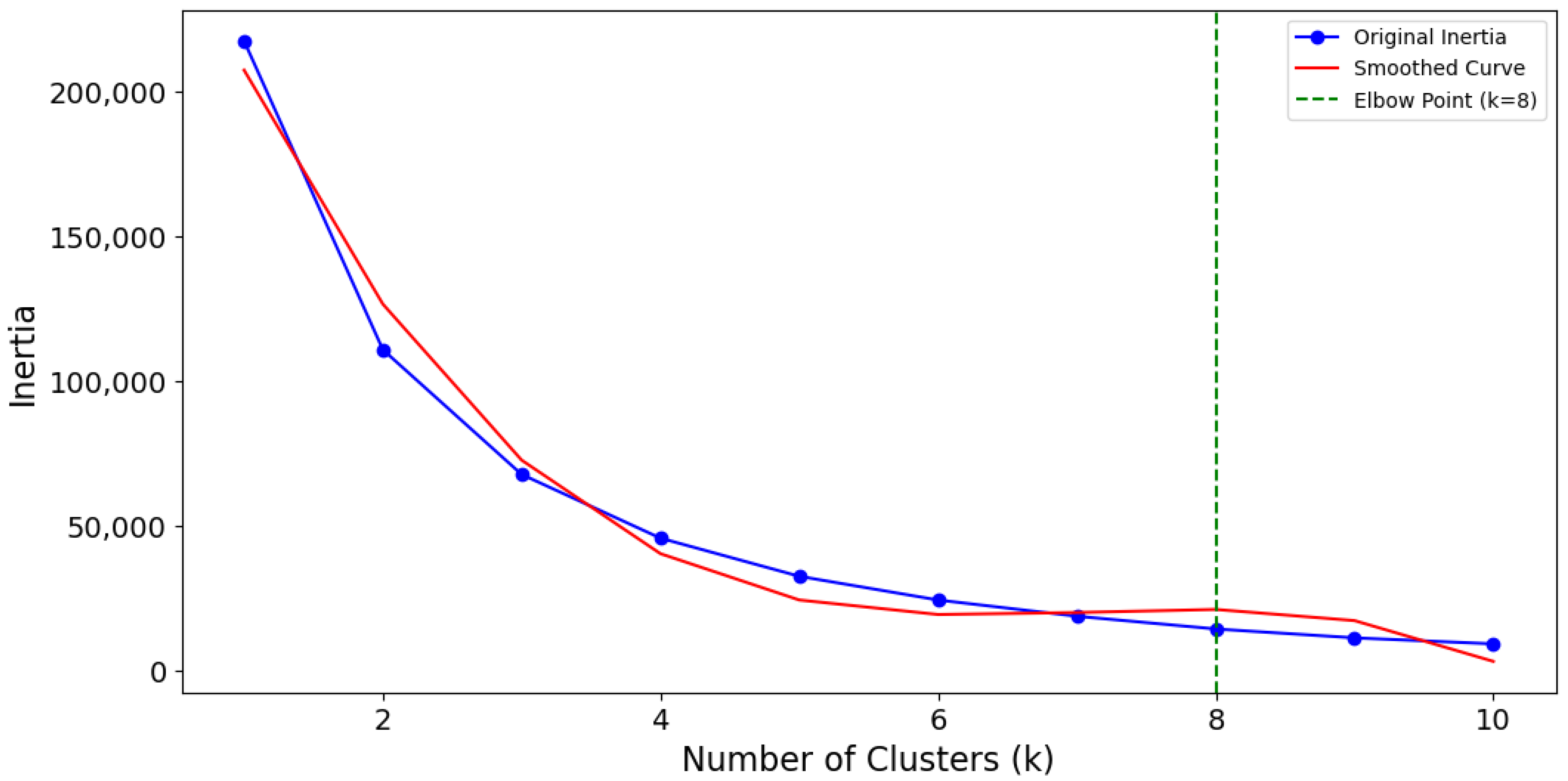
- Initially, the total inertia, also referred to as the Within-Cluster Sum of Squares (WCSS), was computed across a spectrum of k values, indicating the cumulative squared deviations of each data point from the centroid of its corresponding cluster.where
- -
- n is the total number of data points.
- -
- k is the number of clusters evaluated.
- -
- is the i-th data point.
- -
- is the centroid of the j-th cluster.
- Thereafter, to circumvent decisions reliant on the subjective visual analysis of the WCSS curve, a third-degree polynomial was applied to the inertia values. This facilitated the derivation of a continuous mathematical model indicative of the trend of the curve:where
- -
- is the polynomial fitted to the inertia values.
- -
- k represents the number of clusters.
- -
- are the coefficients of the polynomial.
- -
- d is the degree of the polynomial.
- Subsequently, the first and second derivatives of the fitted polynomial were evaluated to ascertain the point of maximum curvature, thereby determining the optimal value of k.where
- -
- represents the first derivative of the fitting polynomial with respect to k.
- -
- represents the second derivative of the polynomial.
- Finally, the curvature radius formula was applied for each value of k, with the aim of quantifying the local curvature of the smoothed curve and finding the point where it reaches its minimum value:where
- -
- is the radius of curvature at each value of k.
2.4.3. Execution of the Clustering Methodology
- Cluster assignment: Each observation is associated with the nearest centroid using Euclidean distance as the metric.
- Centroid update: Centroids are recalculated as the average of the points within each cluster.
- k is the number of defined clusters.
- represents each data point from the set of observations.
- is the set of points assigned to cluster j.
- is the centroid vector corresponding to cluster j.
- denotes the squared Euclidean distance between and .
- is the new centroid of cluster j.
- represents the set of points assigned to cluster j.
- is the total number of points in cluster j.
2.4.4. Assessment of Clustering Model Efficacy
- Firstly, the total inertia metric, also known as the WCSS, is employed to evaluate the internal compactness of each cluster. This metric is computed as the aggregate of the squared distances between each data point and its corresponding centroid:where
- -
- K is the number of clusters.
- -
- is the set of points assigned to cluster k.
- -
- represents each observation within cluster k.
- -
- is the centroid of cluster k.
- -
- is the squared Euclidean distance between point and centroid .
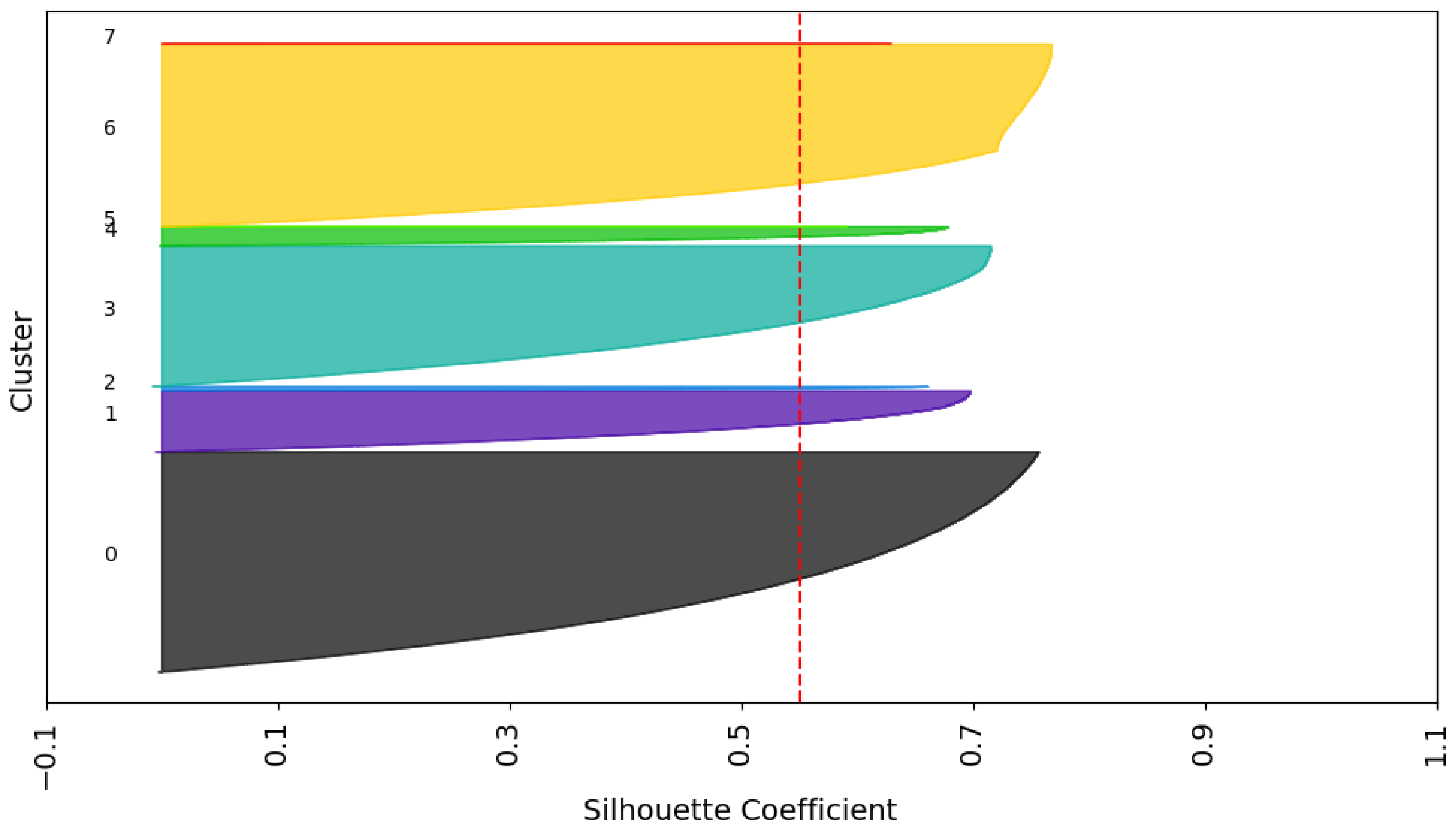
- Secondly, the Silhouette index was utilized, which assesses the similarity degree of each point with its respective cluster in comparison to neighboring clusters. Its value ranges between −1 and +1, with higher values signifying superior separation:where
- -
- is the Silhouette coefficient for point i.
- -
- is the mean distance between point i and all other points in the same cluster.
- -
- is the mean distance between point i and all points in the nearest cluster to which point i does not belong.
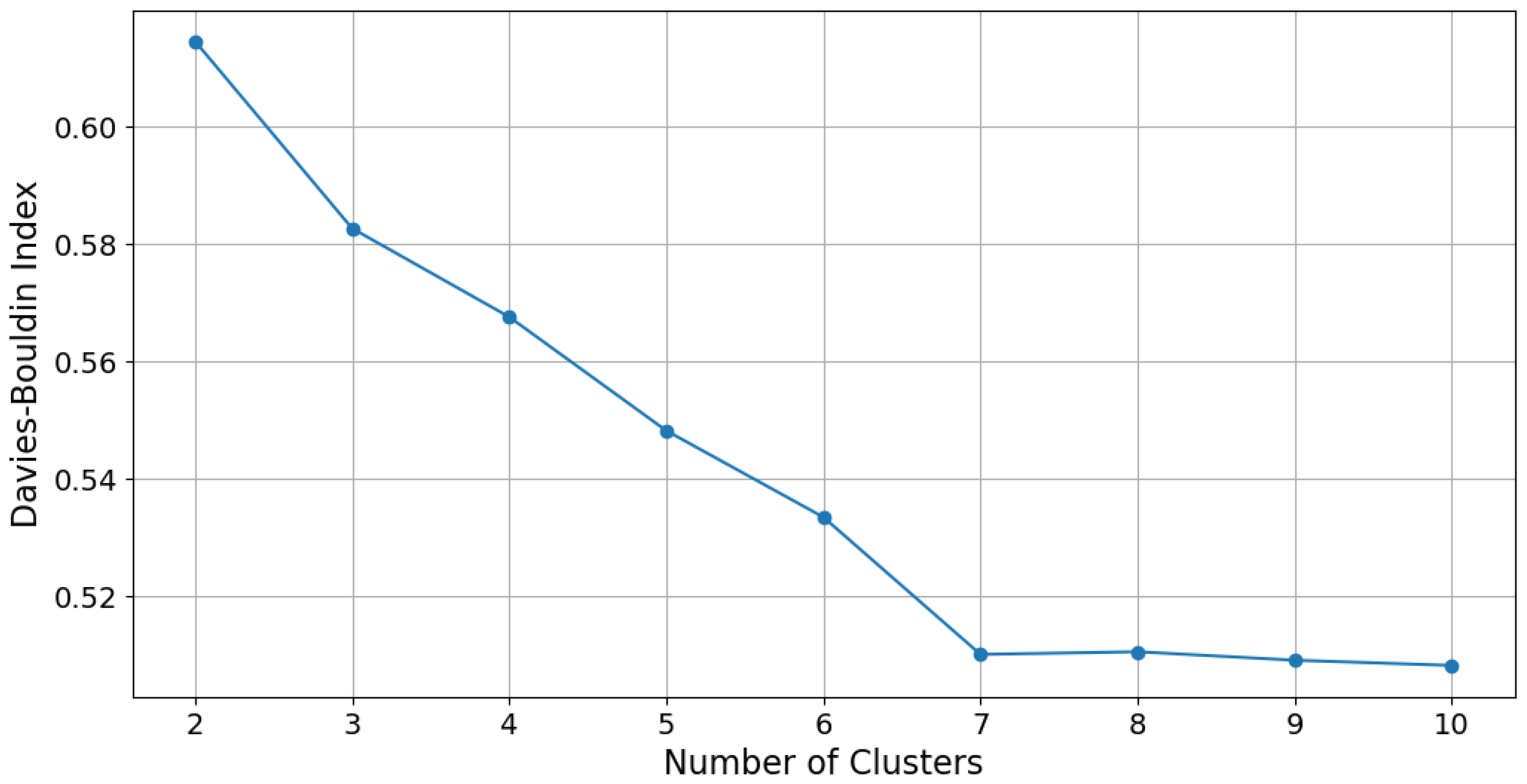
- Finally, Davies–Bouldin (DB) was used, which quantifies the relationship between the dispersion within the clusters and the separation between them. A lower DB value implies a more defined segmentation:where
- -
- is the Davies–Bouldin index.
- -
- k is the number of clusters.
- -
- is the intra-cluster dispersion for cluster i.
- -
- and are the centroids of clusters i and j, respectively.
- -
- is the distance between the centroids of clusters i and j.
2.5. Practical Implementations of the Segmentation Model
2.5.1. Redefinition of Tariffs Based on Consumption Profiles
- In the initial phase, the minimum and maximum consumption thresholds for each cluster are determined as follows:where
- -
- denotes the mean consumption of customer i within cluster .
- -
- and signify the lower and upper limits of cluster , respectively.
- Subsequently, to maintain a consistent sequence in the segments, the clusters were systematically reorganized based on the centroid value:where
- -
- is the centroid of cluster j.
- -
- is the number of clients in cluster j.
- -
- Clusters are reordered according to from smallest to largest.
The new cluster index k is defined as follows:where represents the ordered position of the centroid within the set of clusters.
2.5.2. Detection of Anomalous Consumption Through IQR Analysis
- is the first quartile (25th percentile).
- is the third quartile (75th percentile).
2.5.3. Incorporation of Clustering Techniques Within Demand Forecasting Frameworks
- LR A foundational multiple LR model was constructed to predict future energy consumption through a linear combination of independent variables:where
- -
- Y is the dependent variable (estimated energy consumption).
- -
- are the independent variables (factors such as historical consumption, applied tariff, location, etc.).
- -
- are the regression coefficients, which indicate the influence of each variable .
- -
- is the Y-intercept (value of Y when ).
- -
- is the error or residual term.
- Decision Tree (DT)The decision tree method develops a hierarchical framework of rules systematically partitioning data into homogeneous subsets, employing measures such as entropy or information gain. A primary advantage of this approach is its capacity to model non-linear relationships, alongside its interpretability.where
- -
- is the predicted class.
- -
- is the weight of observation j.
- -
- is an indicator function that is 1 if and 0 otherwise.
Nonetheless, singular DTs are prone to overfitting when confronted with noisy data, which subsequently impacts their generalization capability. - RF To address the issue of overfitting, the RF methodology was implemented. This approach synthesizes multiple DTs, each trained on randomly selected subsets of data and variables. Consequently, the model enhances the stability of predictions and effectively diminishes variance:where
- -
- is the probability that instance X belongs to class y.
- -
- T is the total number of trees in the RF.
- -
- is the prediction of tree t.
- Mean Absolute Error (MAE):where
- -
- is the actual energy consumption value.
- -
- is the value predicted by the model.
- -
- n is the total number of observations.
Lower MAE values indicate better model accuracy. - Root Mean Squared Error (RMSE):where
- -
- is the actual value.
- -
- is the predicted value.
- -
- n is the number of observations.
A low RMSE value indicates a model with more precise predictions and fewer extreme errors. - The Coefficient of Determination ():where
- -
- is the mean of the actual values.
- -
- are the actual values.
- -
- are the predicted values.
An close to 1 indicates a model with high predictive power, while values close to 0 suggest that the model does not explain the variability of the data well.
3. Results
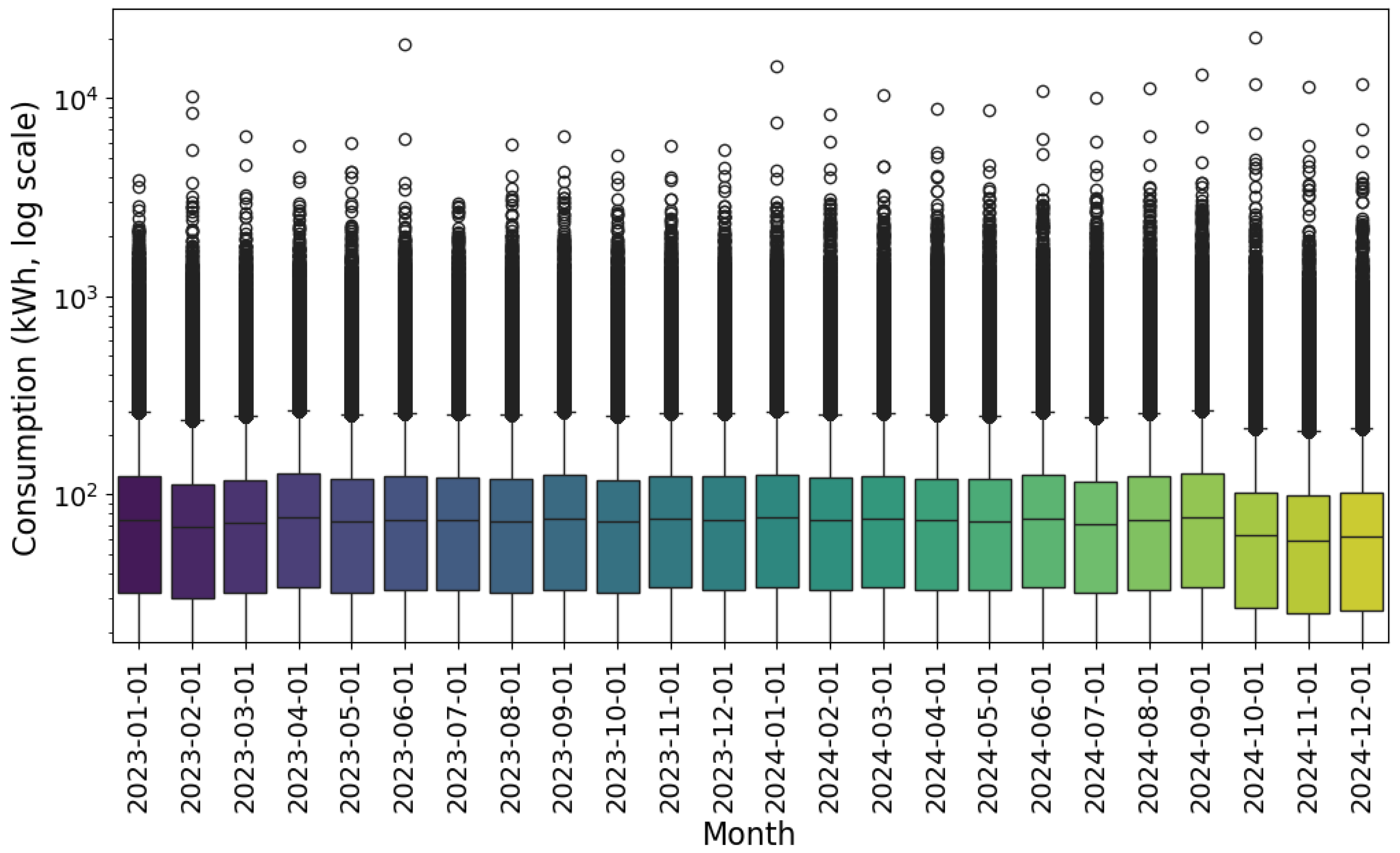
3.1. Descriptive Analysis of the Examined Data
3.2. Determining and Validating the Optimal Quantity of Clusters
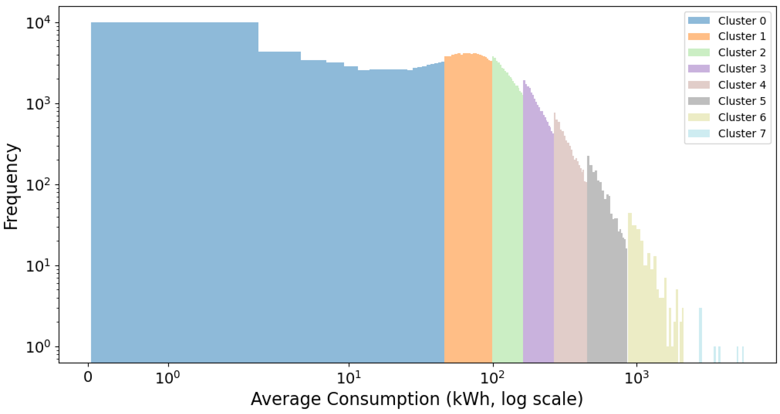
3.3. Examination of the Identified Clusters
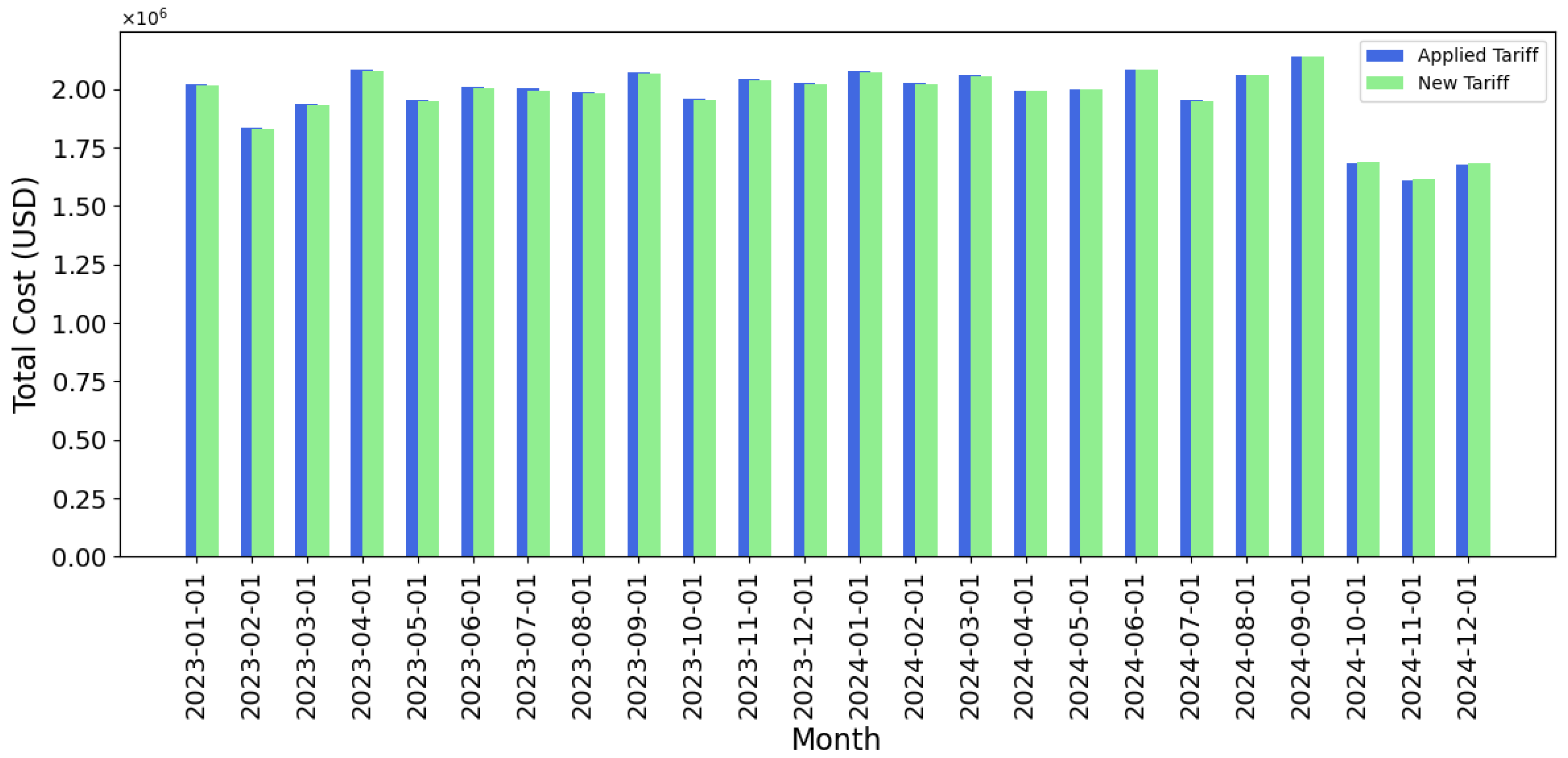
3.4. A Comparative Analysis of Existing and Suggested Rates
- Economic Efficiency: The revised tariff structures are designed to more precisely reflect consumption patterns, thereby enhancing the precision in the allocation of tariff charges and mitigating economic distortions. In addition, as shown in Figure 9, the preservation of total system revenue guarantees the financial stability of the distributor.
- Regulatory Viability: By ensuring that the tariff structure adheres to the boundaries set forth by the national regulatory framework while maintaining anticipated revenue streams, the proposal is technically feasible and can be executed without compromising the operational sustainability of the company.
- Tariff Equity: The categorization of users based on analogous consumption patterns into distinct blocks fortifies the principle of distributive justice. Furthermore, this approach diminishes the number of users situated near pivotal thresholds, consequently reducing incentives for arbitrage and enhancing the perception of transparency within the tariff framework.
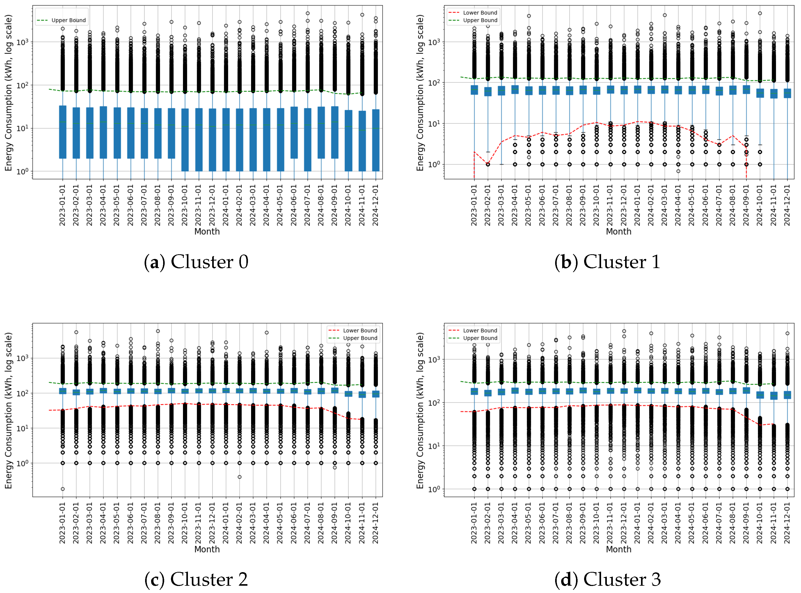
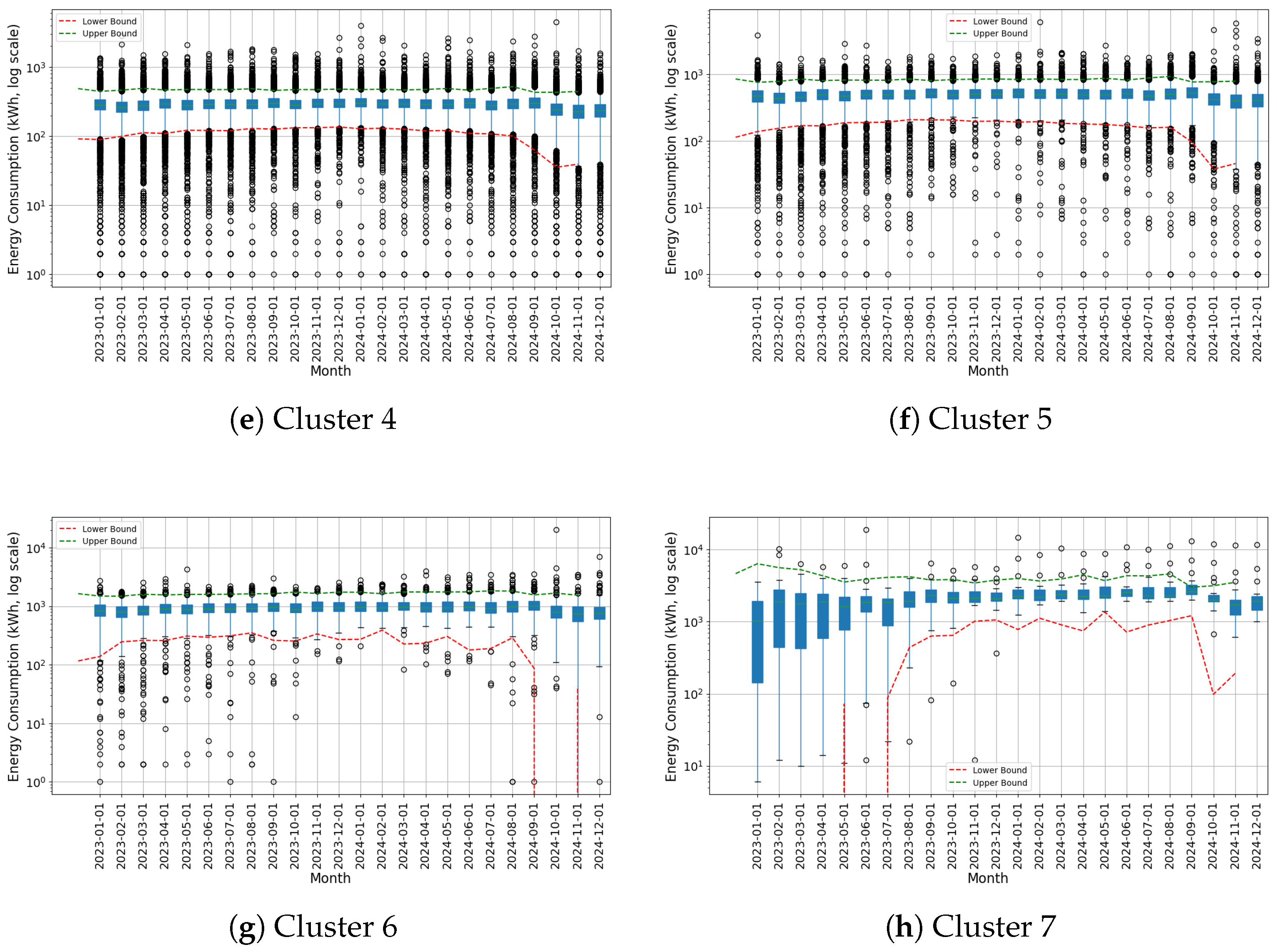
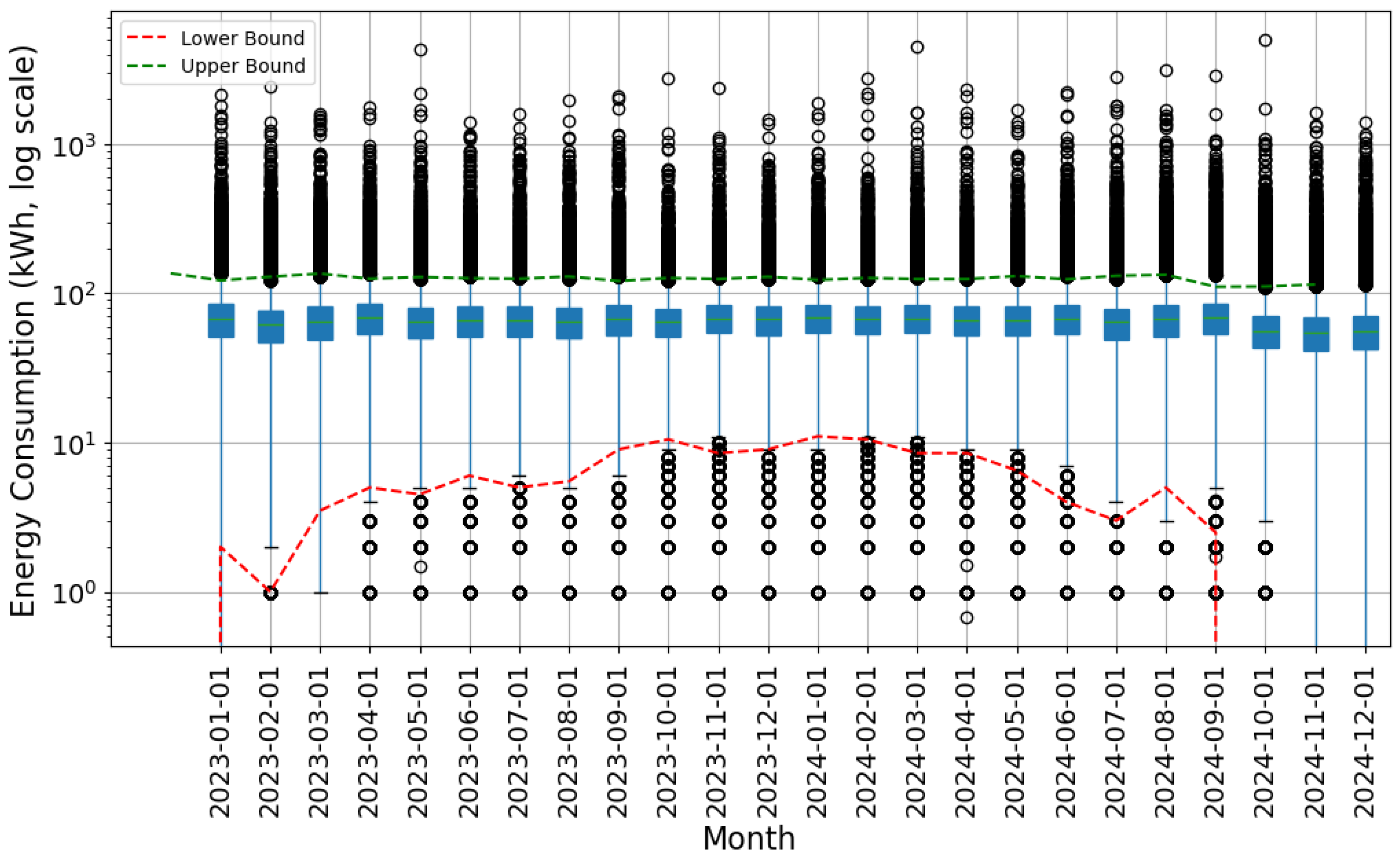
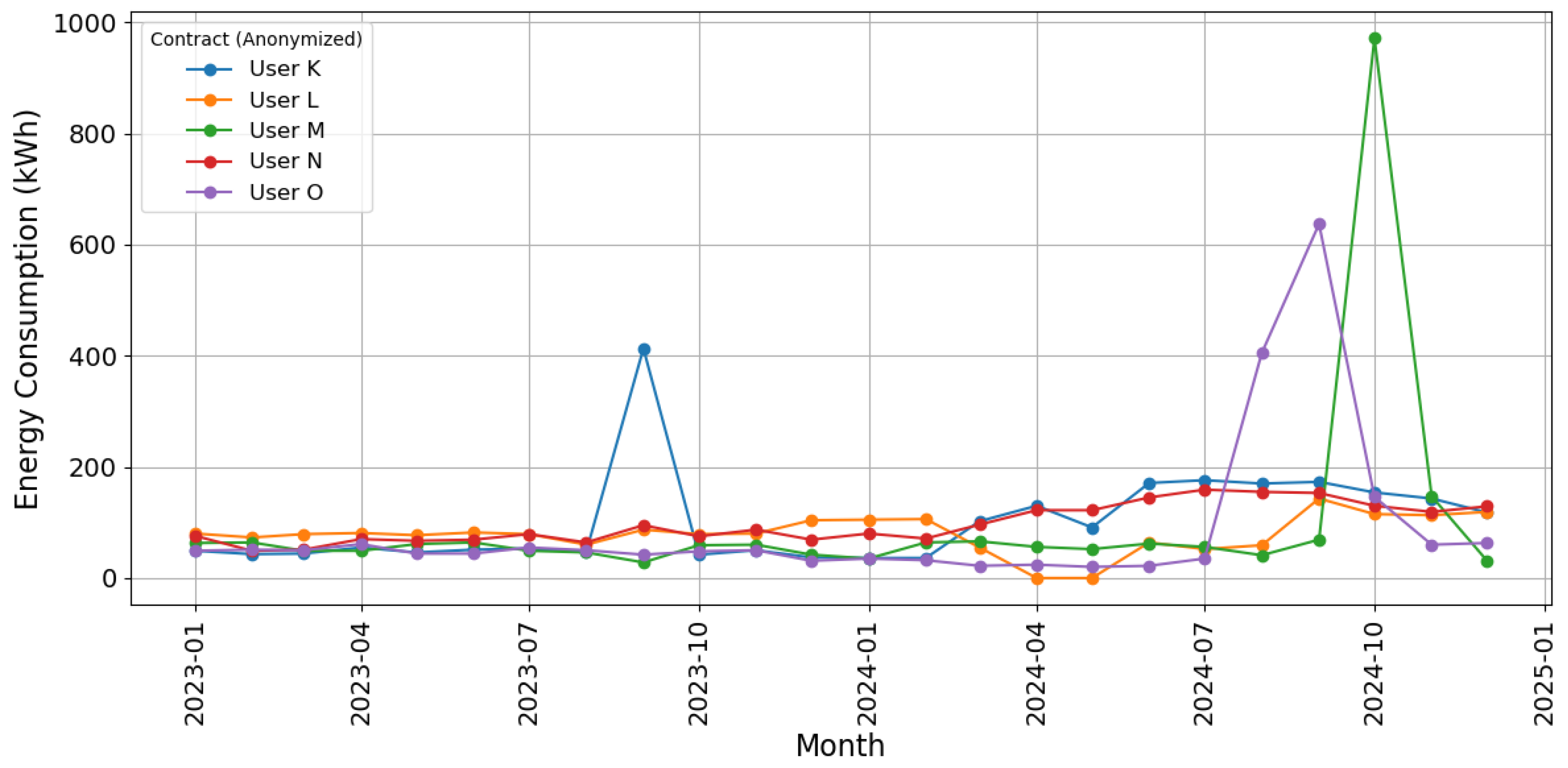
3.5. Outcomes of Anomaly Identification by Cluster
3.6. Assessment of the Efficacy of Predictive Models
4. Discussion
4.1. Assessment of Segmentation Model and Performance
4.2. Comparison with Previous Studies
4.3. Practical Applications: Tariff Formulation, Planning, and Early Detection of Anomalous Consumption
4.4. Limitations of This Study
4.5. Potential Avenues for Enhancement and Future Lines of Inquiry
5. Conclusions
5.1. Validation of the Hypothesis and Methodological Contributions
5.2. Practical Applications for System Planning and Operation
5.3. Restrictions and Recommendations for Future Research
5.4. Principal Contributions of This Research
- Effective Segmentation Without Smart Metering: The model proficiently classified consumers exhibiting uniform consumption behaviors by solely employing monthly billing data.
- Optimization of the Tariff Structure: The reclassification of consumption categories utilizing cluster centroids enhances equity, mitigates economic distortions, and maintains financial sustainability.
- The IQR method effectively facilitated the early detection of anomalous consumption by accurately identifying outliers, thus allowing for prioritized inspections without requiring the installation of smart meters.
- Enhanced Predictive Modeling: By incorporating the cluster as a covariate, the RF model attained an of 0.67, in contrast to 0.12 obtained with LR.
- Practical Applicability and Replicability: The strategy proposed herein is cost-effective, replicable, and adaptable to a wide range of utilities operating within environments where data are limited.
Author Contributions
Funding
Data Availability Statement
Acknowledgments
Conflicts of Interest
Abbreviations
| EEASA | Empresa Eléctrica Ambato Regional Centro Norte S.A. |
| IQR | Interquartile Range |
| WCSS | Within-Cluster Sum of Squares |
| ML | Machine Learning |
| LR | Linear Regression |
| DTs | Decision Trees |
| RF | Random Forest |
Appendix A. Tariff Classification and Description

| No. | Code | Name |
|---|---|---|
| 1 | BTCGSD03 | (BT/Social Assistance) |
| 2 | BTCGCD03 | (BT/Social Assistance with Demand) |
| 3 | NDCGCD01 | (BT/Social Assistance with Hourly Demand) |
| 4 | BTCGSD04 | (BT/Public Benefit) |
| 5 | BTCGCD05 | (BT/Public Benefit with Demand) |
| 6 | BTCGCD20 | (BT/Public Benefit with Hourly Demand) |
| 7 | BTCGCD21 | (BT/Water Pumping for Rural Communities) |
| 8 | BTCGSD14 | (BT/Water Pumping for Public Water Service) |
| 9 | BTCGCD40 | (BT/Water Pumping for Public Water Service with Hourly Demand) |
| 10 | BTCGSD01 | (BT/Commercial) |
| 11 | BTCGCD01 | (BT/Commercial with Demand) |
| 12 | BTCGCD31 | (BT/Commercial with Hourly Demand) |
| 13 | BTCGSD09 | (BT/Religious Worship) |
| 14 | BTCGCD32 | (BT/Religious Worship with Demand) |
| 15 | BTCGSD05 | (BT/Official Entities) |
| 16 | BTCGCD07 | (BT/Official Entities with Demand) |
| 17 | BTCGCD35 | (BT/Official Entities with Hourly Demand) |
| 18 | BTCGCD08 | (BT/Sports Venues with Demand) |
| 19 | BTCGSD02 | (BT/Artisan Industrial) |
| 20 | BTCGCD02 | (BT/Industrial with Demand) |
| 21 | BTCGCD30 | (BT/Industrial with Hourly Demand) |
| 22 | BTCGSD12 | (BT/Sports Venues) |
| 23 | BTCGSD13 | (BT/Water Pumping) |
| 24 | BTCGSD11 | (BT/Community Service) |
| 25 | BTCGCD36 | (BT/Sports Venues with Hourly Demand) |
| 26 | BTCRSD01 | (BT/Residential) |
| 27 | BTCGCD41 | (BT/Electric Vehicles with Hourly Demand) |
| 28 | MTCGCD05 | (MT/Special Subscribers with Demand) |
| 29 | MTCGCD06 | (MT/Special Subscribers with Hourly Demand) |
| 30 | MTCGCD07 | (MT/Social Assistance with Demand) |
| 31 | MTCGCD08 | (MT/Social Assistance with Hourly Demand) |
| 32 | MTCGCD09 | (MT/Public Benefit with Demand) |
| 33 | MTCGCD10 | (MT/Public Benefit with Hourly Demand) |
| 34 | MTCGCD11 | (MT/Water Pumping with Demand) |
| 35 | MTCGCD12 | (MT/Water Pumping with Hourly Demand) |
| 36 | MTCGCD01 | (MT/Commercial with Demand) |
| 37 | MTCGCD02 | (MT/Commercial with Hourly Demand) |
| 38 | MTCGCD13 | (MT/Official Entities with Demand) |
| 39 | MTCGCD14 | (MT/Official Entities with Hourly Demand) |
| 40 | MTCGCD15 | (MT/Sports Venues with Demand) |
| 41 | MTCGCD16 | (MT/Sports Venues with Hourly Demand) |
| 42 | MTCGCD25 | (MT/Fast Charging Station with Differentiated Hourly Demand) |
| 43 | MTCGCD03 | (MT/Industrial with Demand) |
| 44 | MTCGCD32 | (MT/Industrial with Differentiated Hourly Demand) |
| 45 | MTCGCD34 | (MT/Community Service with Hourly Demand) |
| 46 | MTCGCD39 | (MT/Water Pumping for Public Water Service with Hourly Demand) |
| 47 | ATCGCD07 | (AT/Industrial with Differentiated Hourly Demand) |
| 48 | BTCRSD03 | (BT/Residential for PEC Program) |
| 49 | MTCGCD33 | (MT/Religious Worship with Demand) |
Appendix B. Cluster Analysis Results
| Tariff Code | Optimal Clusters | Centroids |
|---|---|---|
| NDCGCD01 | 2 | [2394.43, 2895.9] |
| MTCGCD06 | 2 | [5331.01, 9263.33] |
| BTCGCD40 | 2 | [2399.95, 7418.65] |
| BTCGCD20 | 2 | [2270.96, 5712.8] |
| BTCGCD32 | 2 | [419.4, 2560.62] |
| BTCGCD03 | 3 | [1543.6, 891.0, 2642.58] |
| BTCGCD41 | 3 | [80.62, 159.79, 201.42] |
| BTCGCD08 | 4 | [171.36, 5632.1, 7048.62, 556.2] |
| BTCGCD05 | 4 | [1931.63, 497.42, 2946.97, 1616.7] |
| MTCGCD07 | 4 | [408.89, 1821.18, 3609.1, 1173.09] |
| MTCGCD33 | 4 | [129.41, 326.92, 31.54, 299.28] |
| MTCGCD14 | 5 | [3181.5, 37,063.96, 78,734.7, 129,109.17, 15,625.5] |
| MTCGCD13 | 5 | [282.56, 11,677.47, 4070.26, 1853.76, 6591.21] |
| MTCGCD10 | 5 | [2153.27, 165,376.34, 49,857.05, 19,763.66, 5138.79] |
| BTCGSD13 | 5 | [198.63, 18.91, 1066.88, 385.58, 101.52] |
| MTCGCD09 | 5 | [522.69, 3124.49, 1842.01, 164.14, 1058.21] |
| MTCGCD03 | 5 | [349.85, 2668.15, 10,839.59, 1183.11, 5242.4] |
| MTCGCD01 | 5 | [247.49, 4149.28, 2454.36, 6417.11, 1243.05] |
| BTCGSD14 | 5 | [812.89, 12.5, 300.06, 1085.94, 673.54] |
| MTCGCD32 | 5 | [45,893.64, 1,358,196.0, 4329.7, 506,672.25, 163,288.16] |
| MTCGCD39 | 5 | [5047.56, 531,873.08, 83,837.75, 335,595.17, 39,288.78] |
| BTCGCD01 | 5 | [999.16, 4328.42, 6442.52, 13,346.06, 2500.26] |
| BTCGCD35 | 5 | [3427.68, 25,806.39, 7436.79, 1253.66, 9800.71] |
| BTCGCD02 | 5 | [2110.8, 1040.54, 3546.75, 8462.81, 439.58] |
| BTCGCD21 | 5 | [158.81, 26,779.32, 6890.7, 12,042.01, 1453.09] |
| BTCGCD30 | 5 | [3198.38, 7522.15, 17,195.32, 1241.18, 5261.49] |
| BTCGCD36 | 5 | [5618.13, 496.87, 4970.8, 883.61, 139.4] |
| BTCGSD12 | 5 | [26.25, 1429.3, 409.18, 721.21, 148.47] |
| MTCGCD12 | 6 | [2546.22, 17,676.27, 73.74, 8817.99, 16,204.77, 1479.83] |
| MTCGCD16 | 7 | [89.25, 1639.05, 694.62, 2024.52, 1470.12, 181.94, 655.86] |
| MTCGCD15 | 7 | [54.83, 3990.0, 467.93, 119.28, 194.78, 429.54, 117.38] |
| BTCGSD05 | 8 | [628.38, 2094.26, 42.97, 4716.99, 3422.08, 1201.18, 7659.57, 255.87] |
| BTCGSD04 | 8 | [13.85, 832.42, 186.8, 1797.49, 331.17, 527.47, 1217.01, 85.32] |
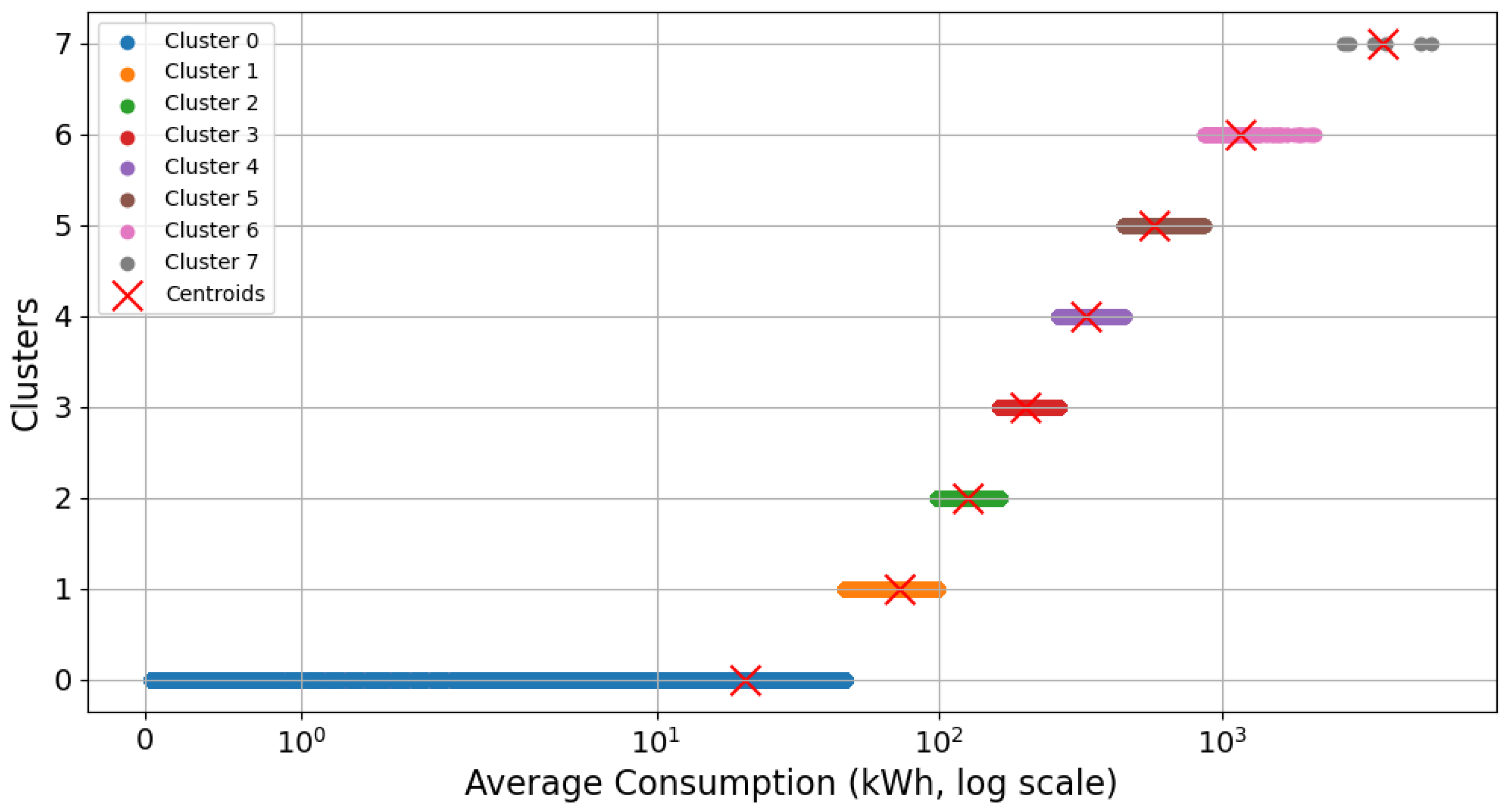
| BTCRSD01 | 8 | [20.63, 72.25, 125.39, 201.52, 328.42, 573.09, 1159.36, 3725.24] |
| BTCGSD03 | 8 | [34.28, 782.41, 2350.22, 333.84, 1577.29, 552.38, 1231.3, 160.32] |
| BTCGCD07 | 9 | [188.97, 3001.96, 5893.12, 1624.22, 1172.06, 3559.69, 2167.13, 724.29, 398.31] |
Appendix C. Consumption Range Analysis Results
| Tariff Code | Consumption Ranges |
|---|---|
| BTCGCD01 | [0, 1687, 3329, 5100, 8620, 14,381, superior] |
| BTCGCD02 | [0, 721, 1527, 2742, 5484, 8462, superior] |
| BTCGCD03 | [0, 890, 1694, 2642, superior] |
| BTCGCD05 | [0, 517, 1616, 1978, 3053, superior] |
| BTCGCD07 | [0, 259, 443, 723, 1173, 1706, 2176, 3062, 3563, 5892, superior] |
| BTCGCD08 | [0, 171, 555, 5631, 7048, superior] |
| BTCGCD20 | [0, 2500, 5712, superior] |
| BTCGCD21 | [0, 613, 2631, 8808, 12748, 29,007, superior] |
| BTCGCD30 | [0, 2176, 4222, 6186, 8521, 17,194, superior] |
| BTCGCD31 | [0, 1149, 2354, 3613, 5425, 7375, 9080, 12,649, 23,056, superior] |
| BTCGCD32 | [0, 487, 2560, superior] |
| BTCGCD35 | [0, 1822, 4518, 7568, 9800, 25,805, superior] |
| BTCGCD36 | [0, 138, 496, 965, 4970, 5617, superior] |
| BTCGCD40 | [0, 2596, 7418, superior] |
| BTCGCD41 | [0, 80, 159, 200, superior] |
| BTCGSD01 | [0, 126, 305, 551, 899, 1409, 2137, 3306, 6785, superior] |
| BTCGSD02 | [0, 111, 238, 412, 669, 1042, 1542, 2328, 3699, superior] |
| BTCGSD03 | [0, 95, 242, 412, 655, 959, 1347, 1576, 2723, superior] |
| BTCGSD04 | [0, 48, 134, 257, 423, 677, 998, 1457, 2245, superior] |
| BTCGSD05 | [0, 148, 439, 904, 1612, 2693, 3865, 4978, 7659, superior] |
| BTCGSD09 | [0, 79, 219, 439, 800, 1064, 1407, 1684, 2673, superior] |
| BTCGSD11 | [0, 57, 164, 322, 507, 848, 1288, 1497, 2031, superior] |
| BTCGSD12 | [0, 85, 255, 530, 930, 1717, superior] |
| BTCGSD13 | [0, 56, 138, 216, 456, 1066, superior] |
| BTCGSD14 | [0, 31, 308, 673, 826, 1113, superior] |
| BTCRSD01 | [0, 45, 98, 162, 264, 450, 863, 2119, 5520, superior] |
| BTCRSD03 | [0, 53, 101, 151, 213, 302, 445, 731, 1523, superior] |
| NDCGCD01 | [0, 2393, 2895, superior] |
| MTCGCD01 | [0, 739, 1844, 3222, 5157, 8161, superior] |
| MTCGCD02 | [0, 3399, 8148, 14,958, 22,692, 33,649, 44,426, 75,424, 277,851, superior] |
| MTCGCD03 | [0, 756, 1895, 3562, 5471, 14,583, superior] |
| MTCGCD06 | [0, 5330, 9262, superior] |
| MTCGCD07 | [0, 429, 1359, 2068, 3608, superior] |
| MTCGCD08 | [0, 6001, 15,648, 32,224, 46,589, 104,668, 147,726, 170,948, 222,813, superior] |
| MTCGCD09 | [0, 299, 631, 1175, 2184, 3789, superior] |
| MTCGCD10 | [0, 3634, 6700, 23,791, 64,368, 165,375, superior] |
| MTCGCD11 | [0, 93, 280, 630, 1058, 1543, 2348, 4211, 18,810, superior] |
| MTCGCD12 | [0, 146, 1479, 2545, 8817, 16,204, 17,675, superior] |
| MTCGCD13 | [0, 1021, 2821, 5141, 7273, 12,383, superior] |
| MTCGCD14 | [0, 9139, 25,234, 46,236, 78,734, 129,108, superior] |
| MTCGCD15 | [0, 54, 116, 119, 194, 429, 467, 3989, superior] |
| MTCGCD16 | [0, 93, 181, 655, 694, 1469, 1638, 2024, superior] |
| MTCGCD32 | [0, 24,461, 86,416, 252,215, 610,251, 1,358,195, superior] |
| MTCGCD33 | [0, 31, 128, 298, 326, superior] |
| MTCGCD39 | [0, 21489, 55,492, 100,345, 335,594, 531,872, superior] |
Appendix D. Cluster Analysis Results for Residential Tariff
References
- Henriques, L.; Lima, F.; Castro, C. Combining Advanced Feature-Selection Methods to Uncover Atypical Energy-Consumption Patterns. Future Internet 2024, 16, 229. [Google Scholar] [CrossRef]
- Ofetotse, E.; Essah, E.; Yao, R. Evaluating the determinants of household electricity consumption using cluster analysis. J. Build. Eng. 2021, 43, 102487. [Google Scholar] [CrossRef]
- AbuBaker, M. Data mining applications in understanding electricity consumers’ behavior: A case study of Tulkarm district, Palestine. Energies 2019, 12, 4287. [Google Scholar] [CrossRef]
- Rathod, R.; Garg, R. Design of electricity tariff plans using gap statistic for K-means clustering based on consumers monthly electricity consumption data. Int. J. Energy Sect. Manag. 2017, 11, 295–310. [Google Scholar] [CrossRef]
- Rajabi, A.; Li, L.; Zhang, J.; Zhu, J.; Ghavidel, S.; Ghadi, M. A review on clustering of residential electricity customers and its applications. In Proceedings of the 2017 20th International Conference on Electrical Machines and Systems, ICEMS 2017, Sydney, Australia, 11–14 August 2017. [Google Scholar] [CrossRef]
- Umar, H.; Prasad, R.; Fonkam, M. Assessing severity of non-technical losses in power using clustering Algorithms. In Proceedings of the 2019 15th International Conference on Electronics, Computer and Computation, ICECCO 2019, Abuja, Nigeria, 10–12 December 2019. [Google Scholar] [CrossRef]
- Miraftabzadeh, S.; Colombo, C.; Longo, M.; Foiadelli, F. K-Means and Alternative Clustering Methods in Modern Power Systems. IEEE Access 2023, 11, 119596–119633. [Google Scholar] [CrossRef]
- Wu, R. Behavioral analysis of electricity consumption characteristics for customer groups using the k-means algorithm. Syst. Soft Comput. 2024, 6, 200143. [Google Scholar] [CrossRef]
- Amri, Y.; Fadhilah, A.; Fatmawati; Setiani, N.; Rani, S. Analysis Clustering of Electricity Usage Profile Using K-Means Algorithm. In Proceedings of the IOP Conference Series: Materials Science and Engineering, Yogyakarta, Indonesia, 11–12 November 2015; Volume 105. [Google Scholar] [CrossRef]
- Kwac, J.; Flora, J.; Rajagopal, R. Lifestyle Segmentation Based on Energy Consumption Data. IEEE Trans. Smart Grid 2018, 9, 2409–2418. [Google Scholar] [CrossRef]
- Sarmas, E.; Fragkiadaki, A.; Marinakis, V. Explainable AI-Based Ensemble Clustering for Load Profiling and Demand Response. Energies 2024, 17, 5559. [Google Scholar] [CrossRef]
- Michalakopoulos, V.; Sarmas, E.; Papias, I.; Skaloumpakas, P.; Marinakis, V.; Doukas, H. A machine learning-based framework for clustering residential electricity load profiles to enhance demand response programs. Appl. Energy 2024, 361, 122943. [Google Scholar] [CrossRef]
- Kaur, R.; Gabrijelčič, D. Behavior segmentation of electricity consumption patterns: A cluster analytical approach. Knowl.-Based Syst. 2022, 251, 109236. [Google Scholar] [CrossRef]
- Fernandes, M.; Viegas, J.; Vieira, S.; Sousa, J. Segmentation of residential gas consumers using clustering analysis. Energies 2017, 10, 2047. [Google Scholar] [CrossRef]
- Toussaint, W.; Moodley, D. Clustering Residential Electricity Consumption Data to Create Archetypes that Capture Household Behaviour in South Africa. S. Afr. Comput. J. 2020, 32, 1–34. [Google Scholar] [CrossRef]
- Wang, S.; Song, A.; Qian, Y. Predicting Smart Cities’ Electricity Demands Using K-Means Clustering Algorithm in Smart Grid. Comput. Sci. Inf. Syst. 2023, 20, 657–678. [Google Scholar] [CrossRef]
- Albayati, A.; Abdullah, N.; Abu-Samah, A.; Mutlag, A.; Nordin, R. Smart grid data management in a heterogeneous environment with a hybrid load forecasting model. Appl. Sci. 2021, 11, 9600. [Google Scholar] [CrossRef]


| Variable | Description | Data Type | Cardinality |
|---|---|---|---|
| date | Consumption record date | Date | 24 |
| contract account | Unique identifier for the customer’s contract | Numeric | 311,625 |
| geographic location | Parish where the customer is located | Categorical | 125 |
| applied tariff | Type of tariff applied to the customer | Categorical | 54 |
| energy consumption | Electrical energy consumption in kWh | Numeric | - |
| Stage | Records Removed | Percentage of Total (%) |
|---|---|---|
| Inactive Accounts (zero consumption) | 21,526 | 6.91 |
| Outliers (negative consumption) | 8978 | 2.88 |
| Non-residential Segments | 59,720 | 19.16 |
| Total Filtered Records | 90,224 | 28.95 |
| Variable | Description | Data Type | Cardinality |
|---|---|---|---|
| date | Consumption record date | Date | 24 |
| contract account | Unique identifier for the customer’s contract | Numeric | 221,401 |
| geographic location | Parish where the customer is located | Categorical | 99 |
| energy consumption | Electrical energy consumption in kWh | Numeric | - |
| Model | WCSS | Silhouette | Davies–Bouldin |
|---|---|---|---|
| K-Means (k = 8) | 20,000 | 0.55 | 0.51 |
| Tariff | Optimal Clusters | Cluster Centroids [kWh] |
|---|---|---|
| Residential | 8 | [20.63, 72.25, 125.39, 201.52, 328.42, 573.09, 1159.36, 3725.24] |
| Tariff | Range | Min Consumption (kWh) | Max Consumption (kWh) | Tariff Charge (USD/kWh) | Average Customers |
|---|---|---|---|---|---|
| BTCRSD01 | 1 | 0.0 | 0.0 | 0 | 13,300 |
| 2 | 1.0 | 45.0 | 0.0900 | 57,760 | |
| 3 | 46.0 | 98.0 | 0.0920 | 71,844 | |
| 4 | 99.0 | 162.0 | 0.0950 | 44,913 | |
| 5 | 163.0 | 264.0 | 0.0976 | 20,606 | |
| 6 | 265.0 | 450.0 | 0.1027 | 6958 | |
| 7 | 451.0 | 863.0 | 0.1285 | 1841 | |
| 8 | 864.0 | 2119.0 | 0.1709 | 287 | |
| 9 | 2120.0 | 5520.0 | 0.4360 | 18 | |
| 10 | 5521.0 | Superior | 0.6812 | 0 |
| Tariff | Range | Min Consumption (kWh) | Max Consumption (kWh) | Tariff Charge (USD/kWh) | Average Customers |
|---|---|---|---|---|---|
| BTCRSD01 | 1 | 0 | 0 | 0 | 13,000 |
| 2 | 0 | 50 | 0.0910 | 77,753 | |
| 3 | 51 | 100 | 0.0930 | 67,410 | |
| 4 | 101 | 150 | 0.0950 | 37,385 | |
| 5 | 151 | 200 | 0.0970 | 16,658 | |
| 6 | 201 | 250 | 0.0990 | 7842 | |
| 7 | 251 | 300 | 0.1010 | 3992 | |
| 8 | 301 | 350 | 0.1030 | 2195 | |
| 9 | 351 | 500 | 0.1050 | 2714 | |
| 10 | 501 | 700 | 0.1285 | 1010 | |
| 11 | 701 | 1000 | 0.1450 | 378 | |
| 12 | 1001 | 1500 | 0.1709 | 142 | |
| 13 | 1501 | 2500 | 0.2752 | 44 | |
| 14 | 2501 | 3500 | 0.4360 | 8 | |
| 15 | 3501 | Superior | 0.6812 | 0 |
| Cluster | Month | Lower Outliers | Upper Outliers |
|---|---|---|---|
| 1 | 1 January 2023 | 0 | 2544 |
| 1 | 1 February 2023 | 1485 | 2513 |
| 1 | 1 March 2023 | 1024 | 2292 |
| 1 | 1 April 2023 | 1448 | 2339 |
| 1 | 1 May 2023 | 1523 | 2278 |
| 1 | 1 June 2023 | 1404 | 2096 |
| 1 | 1 July 2023 | 1350 | 2109 |
| 1 | 1 August 2023 | 1189 | 2016 |
| 1 | 1 September 2023 | 1153 | 1808 |
| 1 | 1 October 2023 | 1301 | 1688 |
| 1 | 1 November 2023 | 1349 | 1513 |
| 1 | 1 December 2023 | 1143 | 1523 |
| 1 | 1 January 2024 | 1132 | 1374 |
| 1 | 1 February 2024 | 1308 | 1607 |
| 1 | 1 March 2024 | 1366 | 1639 |
| 1 | 1 April 2024 | 1469 | 1753 |
| 1 | 1 May 2024 | 1523 | 1636 |
| 1 | 1 June 2024 | 1347 | 1766 |
| 1 | 1 July 2024 | 1394 | 1915 |
| 1 | 1 August 2024 | 1261 | 2074 |
| 1 | 1 September 2024 | 1540 | 2281 |
| 1 | 1 October 2024 | 1536 | 2208 |
| 1 | 1 November 2024 | 0 | 2088 |
| 1 | 1 December 2024 | 0 | 2227 |
| Model | MAE | RMSE | R2 |
|---|---|---|---|
| LR | 6.30 | 8.5 | 0.12 |
| DTs | 25.30 | 67.12 | 0.56 |
| RF | 25.20 | 58.41 | 0.67 |
Disclaimer/Publisher’s Note: The statements, opinions and data contained in all publications are solely those of the individual author(s) and contributor(s) and not of MDPI and/or the editor(s). MDPI and/or the editor(s) disclaim responsibility for any injury to people or property resulting from any ideas, methods, instructions or products referred to in the content. |
© 2025 by the authors. Licensee MDPI, Basel, Switzerland. This article is an open access article distributed under the terms and conditions of the Creative Commons Attribution (CC BY) license (https://creativecommons.org/licenses/by/4.0/).
Share and Cite
Muyulema-Masaquiza, D.; Ayala-Chauvin, M. Segmentation of Energy Consumption Using K-Means: Applications in Tariffing, Outlier Detection, and Demand Prediction in Non-Smart Metering Systems. Energies 2025, 18, 3083. https://doi.org/10.3390/en18123083
Muyulema-Masaquiza D, Ayala-Chauvin M. Segmentation of Energy Consumption Using K-Means: Applications in Tariffing, Outlier Detection, and Demand Prediction in Non-Smart Metering Systems. Energies. 2025; 18(12):3083. https://doi.org/10.3390/en18123083
Chicago/Turabian StyleMuyulema-Masaquiza, Darío, and Manuel Ayala-Chauvin. 2025. "Segmentation of Energy Consumption Using K-Means: Applications in Tariffing, Outlier Detection, and Demand Prediction in Non-Smart Metering Systems" Energies 18, no. 12: 3083. https://doi.org/10.3390/en18123083
APA StyleMuyulema-Masaquiza, D., & Ayala-Chauvin, M. (2025). Segmentation of Energy Consumption Using K-Means: Applications in Tariffing, Outlier Detection, and Demand Prediction in Non-Smart Metering Systems. Energies, 18(12), 3083. https://doi.org/10.3390/en18123083