Exploration of the Ignition Delay Time of RP-3 Fuel Using the Artificial Bee Colony Algorithm in a Machine Learning Framework

Abstract

Ignition delay time (IDT) is a critical parameter for evaluating the autoignition characteristics of aviation fuels. However, its accurate prediction remains challenging due to the complex coupling of temperature, pressure, and compositional factors, resulting in a high-dimensional and nonlinear problem. To address this challenge for the complex aviation kerosene RP-3, this study proposes a multi-stage hybrid optimization framework based on a five-input, one-output BP neural network. The framework—referred to as CGD-ABC-BP—integrates randomized initialization, conjugate gradient descent (CGD), the artificial bee colony (ABC) algorithm, and L2 regularization to enhance convergence stability and model robustness. The dataset includes 700 experimental and simulated samples, covering a wide range of thermodynamic conditions: 624–1700 K, 0.5–20 bar, and equivalence ratios φ = 0.5 − 2.0. To improve training efficiency, the temperature feature was linearized using a 1000/T transformation. Based on 30 independent resampling trials, the CGD-ABC-BP model with a three-hidden-layer structure of [21 17 19] achieved strong performance on internal test data: R² = 0.994 ± 0.001, MAE = 0.04 ± 0.015, MAPE = 1.4 ± 0.05%, and RMSE = 0.07 ± 0.01. These results consistently outperformed the baseline model that lacked ABC optimization. On an entirely independent external test set comprising 70 low-pressure shock tube samples, the model still exhibited strong generalization capability, achieving R² = 0.976 and MAPE = 2.18%, thereby confirming its robustness across datasets with different sources. Furthermore, permutation importance and local gradient sensitivity analysis reveal that the model can reliably identify and rank key controlling factors—such as temperature, diluent fraction, and oxidizer mole fraction—across low-temperature, NTC, and high-temperature regimes. The observed trends align well with established findings in the chemical kinetics literature. In conclusion, the proposed CGD-ABC-BP framework offers a highly accurate and interpretable data-driven approach for modeling IDT in complex aviation fuels, and it shows promising potential for practical engineering deployment.

1. Introduction

Ignition delay time (IDT) is a key parameter for evaluating the autoignition characteristics and ignition propensity of fuels. As a core indicator of fuel autoignition performance, it is widely used in the assessment of combustion behavior in aeroengines and in the development of combustion models. Currently, the most commonly employed techniques for measuring IDT include the shock tube (ST) [1,2,3,4], constant volume combustion bomb (CVCB) [5], and rapid compression machine (RCM) [6,7,8,9]. In addition, with the advancement of optical diagnostic technologies, methods such as laser-induced fluorescence (LIF) and absorption spectroscopy have been incorporated into IDT research [10], significantly enhancing measurement accuracy and temporal resolution. These measurement techniques provide a solid experimental foundation for developing high-precision ignition prediction models. Nevertheless, due to the complex coupling of multiple factors—such as temperature, pressure, equivalence ratio, and molecular structure of the fuel—IDT prediction is characterized by high nonlinearity and dimensionality. Traditional methods based on detailed chemical kinetic mechanisms (e.g., CHEMKIN) [11,12,13,14,15,16,17,18,19] offer reasonable accuracy, but they involve high computational costs during model construction and simulation. Moreover, such approaches are sensitive to initial conditions and are not suitable for real-time engineering applications.

Neural networks—particularly backpropagation (BP) neural networks, as a typical form of feedforward neural networks—have shown strong capability in approximating arbitrary nonlinear functions. In recent years, they have been widely applied for the rapid prediction of ignition delay time (IDT). These data-driven models are typically trained on experimental or simulated datasets to establish nonlinear mapping between input parameters (e.g., initial temperature, pressure, equivalence ratio, oxygen concentration) and the output variable (IDT). Wu et al. [20] employed a three-layer BP neural network using temperature, pressure, and the equivalence ratio as inputs to predict the IDT of various fuels, including methane and n-heptane, achieving a coefficient of determination (R²) greater than 0.98. Liu and Chen [21] extended this approach to alternative aviation fuels, including synthetic and bio-based jet fuels, by constructing a deep feedforward neural network (DNN). Their model achieved superior mean absolute error (MAE) performance over a wider temperature range, maintaining errors below 3 ms. Wang et al. [22] conducted a comparative study using BP neural networks, random forests (RFs), and support vector machines (SVMs) for predicting the IDT of Jet-A surrogate fuels. Their results showed that the BP neural network outperformed the other two models in the mid-to high-temperature range, demonstrating faster training speed and stronger generalization ability. Beyond traditional BP networks, several studies have explored more advanced neural architectures to further enhance model performance. Zhang and Lin [23] proposed a convolutional neural network (CNN)-based approach for capturing local features of temperature, pressure, and compositional inputs, enabling accurate IDT prediction under complex conditions. Patel and Saxena [24] applied a long short-term memory (LSTM) network to model the time-evolving temperature fields and concentration gradients, offering improved dynamic prediction capabilities. Neural-network-based IDT modeling has also been extended to multicomponent aviation fuels such as RP-3 and Jet-A. Cui et al. [25] trained a neural network using experimental data to predict the IDT of RP-3 under ST conditions. Their model achieved prediction errors of less than 5% across a broad range of equivalence ratios and pressures. Ji et al. [26] demonstrated that neural networks optimized using stochastic gradient descent (SGD) can effectively model the pyrolysis of hybrid chemistry mechanisms by learning hundreds of weight parameters. To further improve the interpretability and generalization of neural network models, recent studies have incorporated strategies such as parameter normalization, feature importance analysis (e.g., SHAP values), cross-validation, and transfer learning. These techniques enable neural networks to maintain high predictive accuracy even in small-sample scenarios or for novel fuel systems [27,28].

In summary, the application of neural networks in predicting IDT has progressed from basic single-fuel BP modeling to more advanced composite frameworks that support multi-fuel inputs, diverse network architectures, and high-dimensional feature spaces. Neural networks have become a critical tool for the rapid evaluation of aviation fuels and the optimization of engineering combustion models. In this work, a random selection strategy is adopted to construct and evaluate multiple BP neural networks employing different gradient descent algorithms. Ultimately, a high-precision model based on a hybrid conjugate gradient descent–artificial bee colony (CGD-ABC) optimization strategy is proposed. This model is applied to the fitting and prediction of the IDT of RP-3 fuel under varying conditions of temperature, pressure, and equivalence ratio, offering a reliable data-driven tool for future combustion chamber design and digital twin applications.

2. Materials and Methods

2.1. Data Collection and Preparation

The dataset of RP-3 ignition delay time utilized in this study is sourced from the literature [9,29,30,31,32,33], comprising a total of 700 data points. The temperature range of the dataset spans from 640 to 1600 K, the ambient pressure varies between 0.5 and 20 bar, and the equivalence ratio φ ranges from 0.2 to 2.0. These parameters effectively capture the reaction delay characteristics of RP-3 under diverse combustion conditions. The detailed sources and distribution of the dataset are summarized in

Table 1. Sources and distribution of the IDT dataset.

Data Type	Primary Sources	No. of Samples	T/K	Equivalence Ratio (φ)
Shock-Tube IDT	Zhang 2015 [33]	221	650-1500	1.0, 2.0
	Liu 2022 [30], Liu 2020 [31]	56	1000-1700	0.5, 1.0, 1.5
	Mao 2019 [9]	250	624-1473	0.5, 1.0, 1.5
	Chen 2019 [29]	37	1113-1600	0.5, 1.0, 1.5
	Yang 2021 [32]	29	920-1700	0.5, 1.0, 2.0
RCM IDT	Mao 2019 [9]	107	624-1473	0.5, 1.0, 1.5

.

Among the total samples, 560 were used as the training set (80%), 70 as the validation set (10%), and 70 as the test set (10%). To reduce the magnitude disparity among variables, the ignition delay times in the dataset were logarithmically transformed, and the ignition temperatures were converted using the reciprocal form 1000/T. In addition, the dataset was standardized prior to neural network training to enhance model stability and predictive accuracy. A summary of the preprocessing results for selected samples is presented in

Table 2. Dataset preprocessing.

Number	Diluant (%)	Fuel (%)	Oxidizer (%)	P (bar)	1000/T (K)	Log_Time (μs)	φ
1	79	0.66	20.34	20	0.88	2.25	2
2	79	0.66	20.34	20	0.92	2.46	2
3	79	0.66	20.34	20	0.93	2.50	2
4	79	0.66	20.34	20	0.93	2.48	2
5	79	0.66	20.34	20	0.94	2.54	2
6	79	0.66	20.34	20	0.96	2.63	2
7	79	0.66	20.34	20	1.02	2.92	2
8	79	0.66	20.34	20	0.88	2.26	2
…	…	…	…	…	…	…	…
695	79	2.40	18.60	0.5	0.78	2.64	0.5
696	79	2.40	18.60	0.5	0.81	2.71	0.5
697	79	2.40	18.60	0.5	0.85	3.06	0.5
698	79	2.40	18.60	0.5	0.88	3.16	0.5
699	79	2.40	18.60	0.5	0.90	3.22	0.5
700	79	2.40	18.60	0.5	0.91	3.30	0.5

.

2.2. BP Neural Network Algorithm

The BP neural network is a training algorithm for multilayer feedforward neural networks based on the error backpropagation mechanism (backpropagation algorithm). It is a widely used technique in machine learning for solving tasks such as classification, regression, and function approximation. The BP neural network computes output values through forward propagation and transmits the output error backward layer by layer. During this process, an optimizer is used to iteratively update the network’s weights and biases, thereby minimizing prediction error and improving model performance on the given input data.

In this study, a BP neural network was developed using MATLAB R2024a. The architecture consists of an input layer, a hidden layer, and an output layer. The input layer contains five neurons, corresponding to mixture pressure, ignition temperature, oxidant mole fraction, fuel mole fraction, and diluent mole fraction. The output layer contains a single neuron, representing the IDT. The initial learning rate was set to 0.01, and the minimum error target was set to 0.005. The structural layout of the neural network is illustrated in Figure 1.

In practical modeling scenarios, fixed network configurations—such as the number of hidden layers, neurons per layer, and activation functions—often limit the generalization ability of the model or cause it to converge to local optima. To further enhance the robustness and predictive accuracy of the model, this study adopts a random selection strategy to perform multiple rounds of combination and training on key hyperparameters of the BP neural network.

This strategy comprises the following three components:

(1)

Random sampling of hidden layer neuron counts: For each hidden layer, the number of neurons is randomly sampled from five predefined intervals: [5–15], [15–25], [25–35], [35–45], and [45–55].

(2)

Randomized activation function combinations: The candidate activation functions include tansig (hyperbolic tangent), logsig (logarithmic sigmoid), and purelin (linear function). In each training session, activation functions for the hidden and output layers are randomly assigned to allow flexible adjustment of the model’s nonlinear mapping capability. This strategy is particularly effective in multi-hidden-layer architectures, where it alleviates the limitations associated with single activation functions and enhances overall prediction performance.

(3)

Random perturbation of weight and bias initialization: Network weights and biases are initialized using different random seeds, and each structure undergoes multiple training runs. A model is considered to have good generalization performance if it achieves a coefficient of determination (R²) greater than 0.95, mean absolute error (MAE) less than 0.1, mean absolute percentage error (MAPE) below 4%, and root mean square error (RMSE) below 0.1. Based on these criteria, models are filtered and the configuration with the best generalization performance—according to R², MAE, MAPE, and RMSE—is selected as the candidate model.

2.3. Gradient Descent Algorithm

Gradient descent (GD) is a classical and widely used optimization algorithm, primarily employed to minimize objective functions. It plays a central role in training machine learning and deep learning models. The fundamental idea of GD is to iteratively update model parameters by moving in the direction of the negative gradient of the objective function, gradually approaching the optimal solution.

The following types of GD algorithms are used in this study:

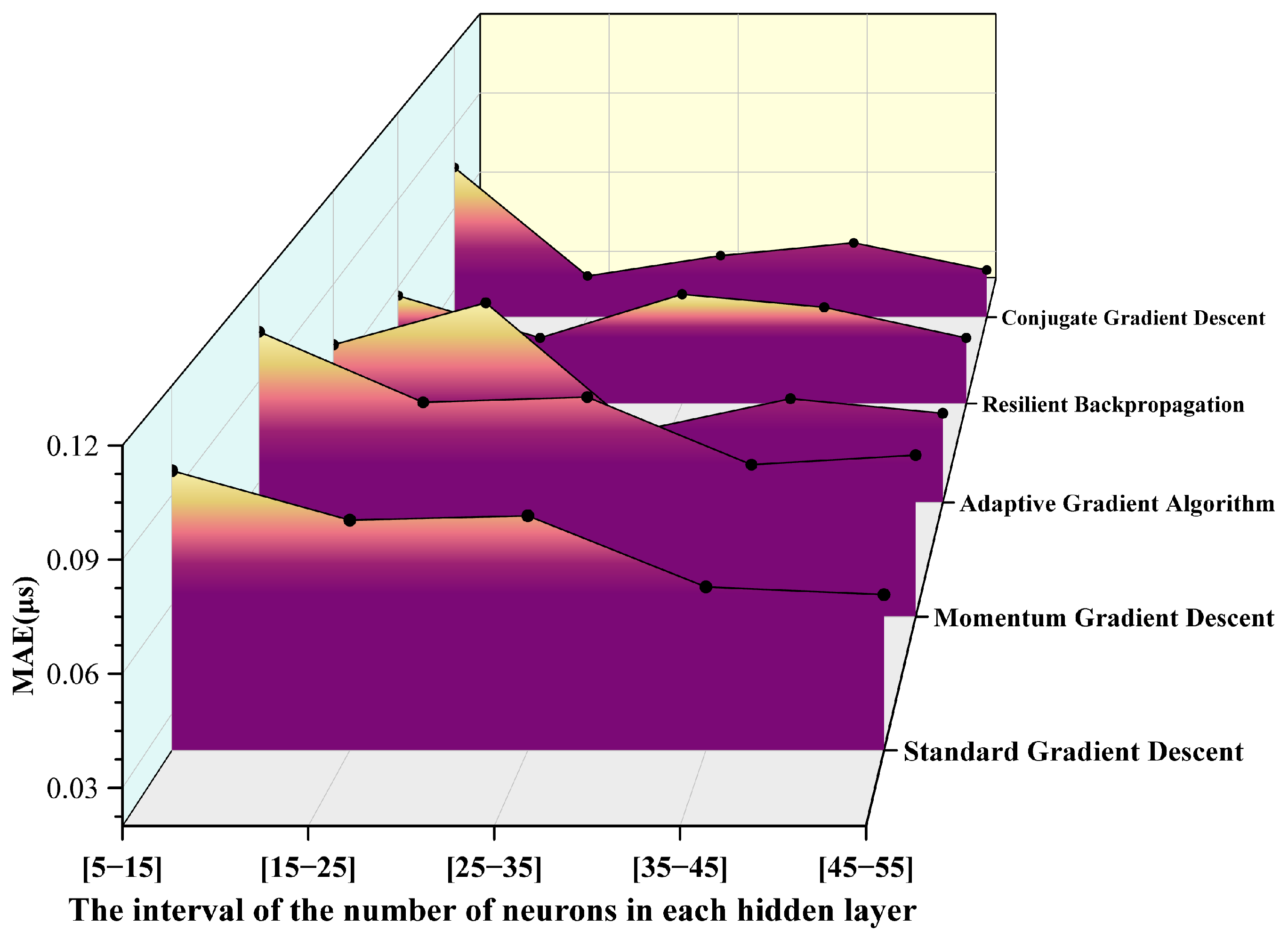
• Standard Gradient Descent (SGD)

SGD is the most basic optimization method in deep learning. It updates model parameters based on the gradient of the loss function with respect to the parameters. The update rule is given using the following equation:

$${\mathrm{\theta }}^{\left(\mathrm{t}+1\right)}={\mathrm{\theta }}^{\left(\mathrm{t}\right)}-\mathrm{\eta }\cdot {\nabla }_{\mathrm{\theta }}\mathrm{J}\left({\mathrm{\theta }}^{\left(\mathrm{t}\right)}\right)$$

(1)

where $\mathrm{\theta }$ denotes the model parameters, $\mathrm{\eta }$ represents the learning rate, and ${\nabla }_{\mathrm{\theta }}\mathrm{J}\left(\mathrm{\theta }\right)$ stands for the gradient of the loss function with respect to the parameters for the current batch of samples.

2.

Momentum Gradient Descent (MGD)

To address the slow convergence of SGD in regions with high curvature or non-convexity, the momentum term is introduced. Inspired by the concept of physical inertia, this method combines current and historical gradient information to suppress oscillations and accelerate convergence. The computation is defined by Equations (2) and (3).

$${\mathrm{v}}^{\left(\mathrm{t}\right)}=\mathrm{\gamma }{\mathrm{v}}^{\left(\mathrm{t}-1\right)}+\mathrm{\eta }\cdot {\nabla }_{\mathrm{\theta }}\mathrm{J}\left({\mathrm{\theta }}^{\left(\mathrm{t}\right)}\right)$$

(2)

$${\mathrm{\theta }}^{\left(\mathrm{t}+1\right)}={\mathrm{\theta }}^{\left(\mathrm{t}\right)}-{\mathrm{v}}^{\left(\mathrm{t}\right)}$$

(3)

where ${\mathrm{v}}^{\left(\mathrm{t}\right)}$ represents the accumulated momentum, and $\mathrm{\gamma }\in \left[0,1\right)$ denotes the momentum factor, which is typically set to 0.9.

3.

Adaptive Gradient Algorithm (AGA)

The adaptive gradient algorithm designs an individual learning rate for each parameter, adjusting the step size based on the accumulated history of past gradients. This feature is particularly advantageous when handling sparse data or features of varying importance. The calculation formulas are presented in Equations (4) and (5).

$${\mathrm{G}}_{\mathrm{t}}={\mathrm{G}}_{\mathrm{t}-1}+{\nabla }_{\mathrm{\theta }}\mathrm{J}{\left({\mathrm{\theta }}^{\left(\mathrm{t}\right)}\right)}^2$$

(4)

$${\mathrm{\theta }}^{\left(\mathrm{t}+1\right)}={\mathrm{\theta }}^{\left(\mathrm{t}\right)}-{\displaystyle \frac{\mathrm{\eta }}{\sqrt{{\mathrm{G}}_{\mathrm{t}}+\mathrm{ϵ}}}}\cdot {\nabla }_{\mathrm{\theta }}\mathrm{J}\left({\mathrm{\theta }}^{\left(\mathrm{t}\right)}\right)$$

(5)

where ${\mathrm{G}}_{\mathrm{t}}$ denotes the accumulation of squared historical gradients for each parameter; $\mathrm{ϵ}$ is a very small constant introduced to avoid division by zero; $\mathrm{\eta }$ represents the initial learning rate; and ${\nabla }_{\mathrm{\theta }}\mathrm{J}\left({\mathrm{\theta }}^{\left(\mathrm{t}\right)}\right)$ indicates the current gradient.

4.

Resilient Backpropagation (RPROP)

Traditional BP relies on GD to update weights based on the gradient magnitude, but often suffers from issues such as vanishing or exploding gradients and sensitivity to learning rate. RPROP addresses these problems by considering only the sign of the gradient to determine the update direction, while the step size is adjusted adaptively for each weight. The calculation method is provided by Equations (6) and (7).

$${\Delta }_{\mathrm{i}\mathrm{j}}^{\left(\mathrm{t}\right)}\&=\left\{\begin{array}{ccc}\mathrm{m}\mathrm{i}\mathrm{n}({\Delta }_{\mathrm{i}\mathrm{j}}^{(\mathrm{t}-1)}\cdot {\mathrm{\eta }}^{+},{\Delta }_{\mathrm{m}\mathrm{a}\mathrm{x}})& \mathrm{i}\mathrm{f}{{\displaystyle \frac{\partial \mathrm{E}}{\partial {\mathrm{w}}_{\mathrm{i}\mathrm{j}}}}}^{\left(\mathrm{t}\right)}\cdot {{\displaystyle \frac{\partial \mathrm{E}}{\partial {\mathrm{w}}_{\mathrm{i}\mathrm{j}}}}}^{(\mathrm{t}-1)}>0& \\ \mathrm{m}\mathrm{a}\mathrm{x}({\Delta }_{\mathrm{i}\mathrm{j}}^{(\mathrm{t}-1)}\cdot {\mathrm{\eta }}^{-},{\Delta }_{\mathrm{m}\mathrm{i}\mathrm{n}})& \mathrm{i}\mathrm{f}{{\displaystyle \frac{\partial \mathrm{E}}{\partial {\mathrm{w}}_{\mathrm{i}\mathrm{j}}}}}^{\left(\mathrm{t}\right)}\cdot {{\displaystyle \frac{\partial \mathrm{E}}{\partial {\mathrm{w}}_{\mathrm{i}\mathrm{j}}}}}^{(\mathrm{t}-1)}<0& \\ {\Delta }_{\mathrm{i}\mathrm{j}}^{(\mathrm{t}-1)}& \mathrm{o}\mathrm{t}\mathrm{h}\mathrm{e}\mathrm{r}\mathrm{w}\mathrm{i}\mathrm{s}\mathrm{e}& \end{array}\right.$$

(6)

$$\begin{array}{c}\Delta {\mathrm{w}}_{\mathrm{i}\mathrm{j}}^{\left(\mathrm{t}\right)}=\left\{\begin{array}{ccc}-{\Delta }_{\mathrm{i}\mathrm{j}}^{\left(\mathrm{t}\right)}& \mathrm{i}\mathrm{f}{{\displaystyle \frac{\partial \mathrm{E}}{\partial {\mathrm{w}}_{\mathrm{i}\mathrm{j}}}}}^{\left(\mathrm{t}\right)}>0& \\ +{\Delta }_{\mathrm{i}\mathrm{j}}^{\left(\mathrm{t}\right)}& \mathrm{i}\mathrm{f}{{\displaystyle \frac{\partial \mathrm{E}}{\partial {\mathrm{w}}_{\mathrm{i}\mathrm{j}}}}}^{\left(\mathrm{t}\right)}<0& \\ 0& \mathrm{i}\mathrm{f}{{\displaystyle \frac{\partial \mathrm{E}}{\partial {\mathrm{w}}_{\mathrm{i}\mathrm{j}}}}}^{\left(\mathrm{t}\right)}=0& \end{array}\right.\\ {\mathrm{w}}_{\mathrm{i}\mathrm{j}}^{(\mathrm{t}+1)}={\mathrm{w}}_{\mathrm{i}\mathrm{j}}^{\left(\mathrm{t}\right)}+\Delta {\mathrm{w}}_{\mathrm{i}\mathrm{j}}^{\left(\mathrm{t}\right)}\end{array}$$

(7)

where ${\Delta }_{\mathrm{i}\mathrm{j}}$ is the update step size for weight ${\mathrm{w}}_{\mathrm{i}\mathrm{j}}$; ${\mathrm{\eta }}^{+}$ and ${\mathrm{\eta }}^{-}$ are the increase and decrease factors, respectively; and ${\Delta }_{\max }$ and ${\Delta }_{\min }$ define the upper and lower bounds for the step size.

5.

Conjugate Gradient Descent (CGD)

The conjugate gradient method was initially developed for solving large-scale linear systems and has been adapted for use in neural networks as an approximate second-order optimization algorithm. Unlike traditional first-order methods, it avoids the explicit storage of the full Hessian matrix. Compared to stochastic gradient descent (SGD), the conjugate gradient method demonstrates a faster convergence rate. Its fundamental update rules are presented in Equations (8)–(10).

$${\mathrm{x}}_{\mathrm{k}+1}={\mathrm{x}}_{\mathrm{k}}+{\mathrm{\alpha }}_{\mathrm{k}}{\mathrm{d}}_{\mathrm{k}}$$

(8)

$${\mathrm{d}}_{\mathrm{k}}=-\nabla \mathrm{f}\left({\mathrm{x}}_{\mathrm{k}}\right)+\left({\displaystyle \frac{\nabla \mathrm{f}{\left({\mathrm{x}}_{\mathrm{k}}\right)}^{\mathrm{T}}\nabla \mathrm{f}\left({\mathrm{x}}_{\mathrm{k}}\right)}{\nabla \mathrm{f}{\left({\mathrm{x}}_{\mathrm{k}-1}\right)}^{\mathrm{T}}\nabla \mathrm{f}\left({\mathrm{x}}_{\mathrm{k}-1}\right)}}\right){\mathrm{d}}_{\mathrm{k}-1}$$

(9)

$${\mathrm{\alpha }}_{\mathrm{k}}=\mathrm{a}\mathrm{r}\mathrm{g}\underset{\mathrm{\alpha }}{\mathrm{m}\mathrm{i}\mathrm{n}}\mathrm{f}\left({\mathrm{x}}_{\mathrm{k}}+\mathrm{\alpha }{\mathrm{d}}_{\mathrm{k}}\right)$$

(10)

where $\mathrm{f}\left(\mathrm{x}\right)$ represents the objective function, ${\mathrm{x}}_{\mathrm{k}}$ denotes the iteration variable, $\nabla \mathrm{f}\left({\mathrm{x}}_{\mathrm{k}}\right)$ signifies the gradient, ${\mathrm{d}}_{\mathrm{k}}$ corresponds to the conjugate direction, and ${\mathrm{\alpha }}_{\mathrm{k}}$ indicates the step size.

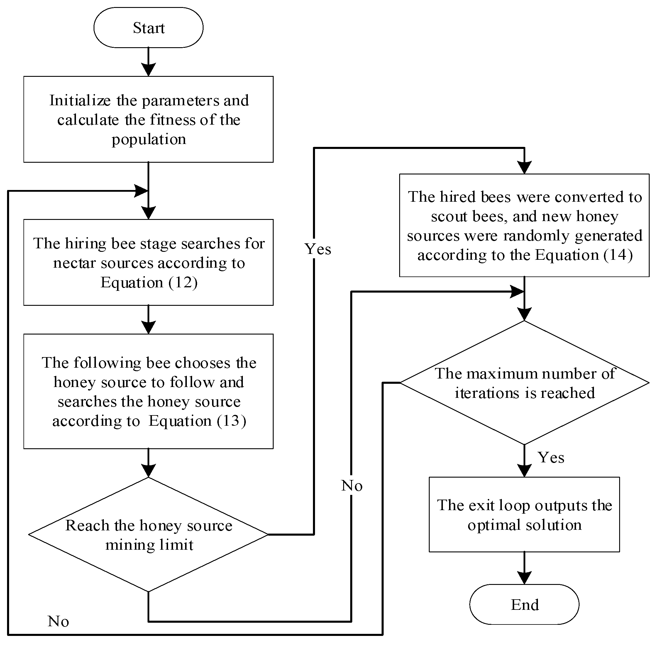
2.4. Artificial Bee Colony Algorithm

The artificial bee colony (ABC) algorithm is a swarm intelligence optimization method inspired by the foraging behavior of honeybees. It was first proposed by Karaboga in 2005. The algorithm mimics the process of bees searching for, sharing information about, and abandoning food sources, thereby enabling global exploration of the solution space. It is characterized by its simple structure, few control parameters, and strong global search capability, making it particularly suitable for avoiding local optima in neural network training.

In the ABC algorithm, each individual bee represents a potential solution—for example, a parameter vector of a neural network—and the quality of each solution is evaluated using a fitness function. In neural network optimization, the fitness function is typically defined as the model’s prediction error, such as the mean squared error (MSE):

$$\mathrm{MSE}={\displaystyle \frac{1}{\mathrm{n}}}\sum _{\mathrm{i}=1}^{\mathrm{n}}{\left({\mathrm{y}}_{\mathrm{i}}-\widehat{{\mathrm{y}}_{\mathrm{i}}}\right)}^2$$

(11)

where ${\mathrm{y}}_{\mathrm{i}}$ is the true value, $\widehat{{\mathrm{y}}_{\mathrm{i}}}$ is the predicted value by the neural network, and n is the number of samples. A smaller MSE indicates better model performance and higher predictive accuracy.

The ABC algorithm involves three types of bees: employed bees, onlooker bees, and scout bees. Employed bees generate new solutions around the current food source (i.e., the current solution) using the perturbation defined in Equation (12).

$${\mathrm{v}}_{\mathrm{i}\mathrm{j}}={\mathrm{x}}_{\mathrm{i}\mathrm{j}}+{\mathrm{\varphi }}_{\mathrm{i}\mathrm{j}}\left({\mathrm{x}}_{\mathrm{i}\mathrm{j}}-{\mathrm{x}}_{\mathrm{k}\mathrm{j}}\right)$$

(12)

where ${\mathrm{x}}_{\mathrm{i}\mathrm{j}}$ represents the j-th parameter of the i-th bee, ${\mathrm{x}}_{\mathrm{k}\mathrm{j}}$ is the j-th parameter of another randomly selected bee, and ${\mathrm{\varphi }}_{\mathrm{i}\mathrm{j}}$ is a random number in the range [−1,1]. This operation enables local search by moving closer to or farther from other bees’ parameters, thereby balancing exploration and exploitation.

Onlooker bees select food sources probabilistically based on their fitness values. The probability of participating in the optimization process is defined by Equation (13).

$${\mathrm{p}}_{\mathrm{i}}={\displaystyle \frac{\mathrm{f}\mathrm{i}{\mathrm{t}}_{\mathrm{i}}}{{\sum }_{\mathrm{j}=1}^{\mathrm{N}}\mathrm{f}\mathrm{i}{\mathrm{t}}_{\mathrm{j}}}}$$

(13)

where $\mathrm{f}\mathrm{i}{\mathrm{t}}_{\mathrm{i}}$ denotes the fitness value of the i-th solution, and N represents the total number of bees. This mechanism encourages more bees to cluster around better solutions, thereby improving the accuracy of the search process.

If a food source fails to generate a better solution after a specified number of iterations (denoted as limit), it is considered exhausted and will be abandoned. The corresponding employed bee will then transform into a scout bee, which randomly generates a new food source within the search space. The new solution is calculated according to Equation (14):

$${\mathrm{x}}_{\mathrm{i}\mathrm{j}}={\mathrm{x}}_{\mathrm{j}}^{\mathrm{m}\mathrm{i}\mathrm{n}}+\mathrm{r}\mathrm{a}\mathrm{n}\mathrm{d}\left(0,1\right)·\left({\mathrm{x}}_{\mathrm{j}}^{\mathrm{m}\mathrm{a}\mathrm{x}}-{\mathrm{x}}_{\mathrm{j}}^{\mathrm{m}\mathrm{i}\mathrm{n}}\right)$$

(14)

This step is equivalent to introducing a mutation mechanism, which maintains population diversity and enhances the global search capability. A detailed flowchart of the algorithm is shown in Figure 2.

2.5. Evaluation of Models

After training, the BP neural network generally requires the evaluation of its prediction performance and generalization ability using a set of metrics. To comprehensively assess the performance of the delayed ignition time prediction model, this paper selected several widely used evaluation metrics in regression analysis. These include MAE, MAPE, RMSE, and R². These metrics assess the model from multiple perspectives, such as predictive accuracy, stability, and the degree of fit to ground truth data. They also provide a quantitative basis for model tuning and practical engineering application.

MAE is one of the most fundamental regression evaluation metrics. It represents the average of the absolute differences between the predicted values and the actual values. MAE treats all errors equally without emphasizing outliers, and a smaller MAE indicates a more accurate model. Its calculation method is provided in Equation (15).

$$\mathrm{M}\mathrm{A}\mathrm{E}={\displaystyle \frac{1}{\mathrm{n}}}\sum _{\mathrm{i}=1}^{\mathrm{n}}\left|{\mathrm{y}}_{\mathrm{i}}-\widehat{{\mathrm{y}}_{\mathrm{i}}}\right|$$

(15)

where ${\mathrm{y}}_{\mathrm{i}}$ is the actual value of the i-th sample, $\widehat{{\mathrm{y}}_{\mathrm{i}}}$ is the predicted value, and n is the total number of samples.

In contrast, the MAPE further standardizes the error by expressing it as a percentage relative to the true value, as calculated in Equation (16).

$$\mathrm{M}\mathrm{A}\mathrm{P}\mathrm{E}={\displaystyle \frac{100\%}{\mathrm{n}}}\sum _{\mathrm{i}=1}^{\mathrm{n}}\left|{\displaystyle \frac{{\mathrm{y}}_{\mathrm{i}}-\widehat{{\mathrm{y}}_{\mathrm{i}}}}{{\mathrm{y}}_{\mathrm{i}}}}\right|$$

(16)

In addition, R² is an important metric for evaluating the goodness of fit of a model. It reflects the proportion of the variance in the dependent variable that can be explained by the independent variables. An R² value closer to 1 indicates a better fit, whereas a negative R² implies that the model performs worse than simply predicting the mean of the observed values. The calculation of R² is presented in Equation (17).

$${\mathrm{R}}^2=1-{\displaystyle \frac{{\sum }_{\mathrm{i}=1}^{\mathrm{n}}{\left({\mathrm{y}}_{\mathrm{i}}-\widehat{{\mathrm{y}}_{\mathrm{i}}}\right)}^2}{{\sum }_{\mathrm{i}=1}^{\mathrm{n}}{\left({\mathrm{y}}_{\mathrm{i}}-\overline{\mathrm{y}}\right)}^2}}$$

(17)

where $\overline{\mathrm{y}}$ represents the mean of the true values.

However, during the model construction and training process, it was found that the above three metrics (MAE, MAPE, and R²) may not sufficiently reflect the model’s performance when dealing with outliers. Therefore, RMSE is introduced as an additional evaluation metric to provide a more comprehensive assessment of the model’s predictive performance. RMSE incorporates the squared differences between predictions and actual values before applying the square root, thereby placing greater emphasis on larger errors. Due to its sensitivity to outliers, RMSE is particularly suitable for evaluating models where high accuracy is required, especially in scenarios involving occasional extreme events (e.g., unusually long ignition delay times). The calculation method for RMSE is provided in Equation (18).

$$\mathrm{R}\mathrm{M}\mathrm{S}\mathrm{E}=\sqrt{{\displaystyle \frac{1}{\mathrm{n}}}\sum _{\mathrm{i}=1}^{\mathrm{n}}{\left({\mathrm{y}}_{\mathrm{i}}-\widehat{{\mathrm{y}}_{\mathrm{i}}}\right)}^2}$$

(18)

By adopting these four evaluation metrics—MAE, MAPE, RMSE, and R²—this study enables a multidimensional assessment of model performance from the perspectives of error magnitude, relative deviation, goodness of fit, and outlier sensitivity. This provides a robust and scientific basis for further model refinement and practical engineering application.

3. Results

3.1. Determination of Hyperparameter Ranges

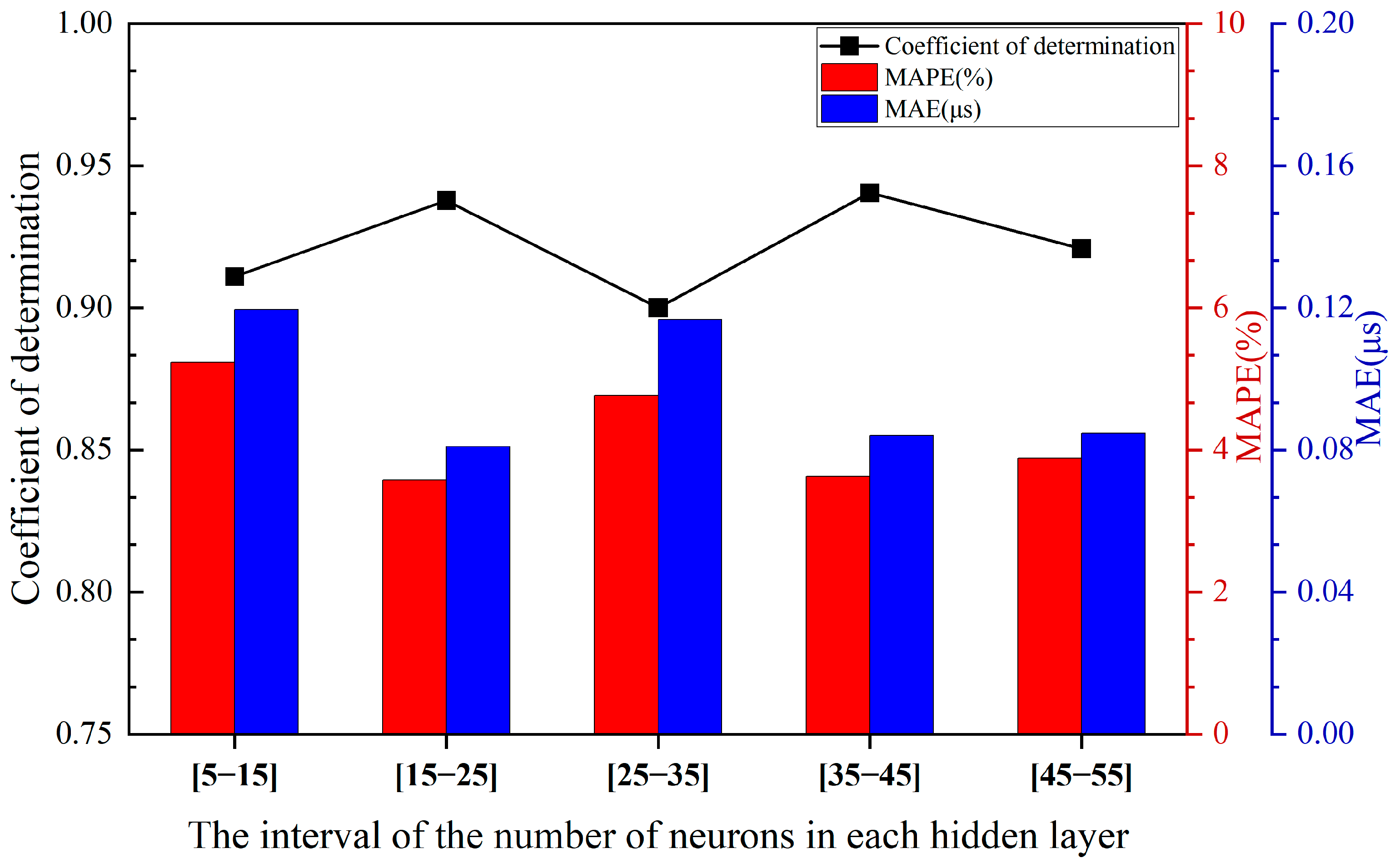
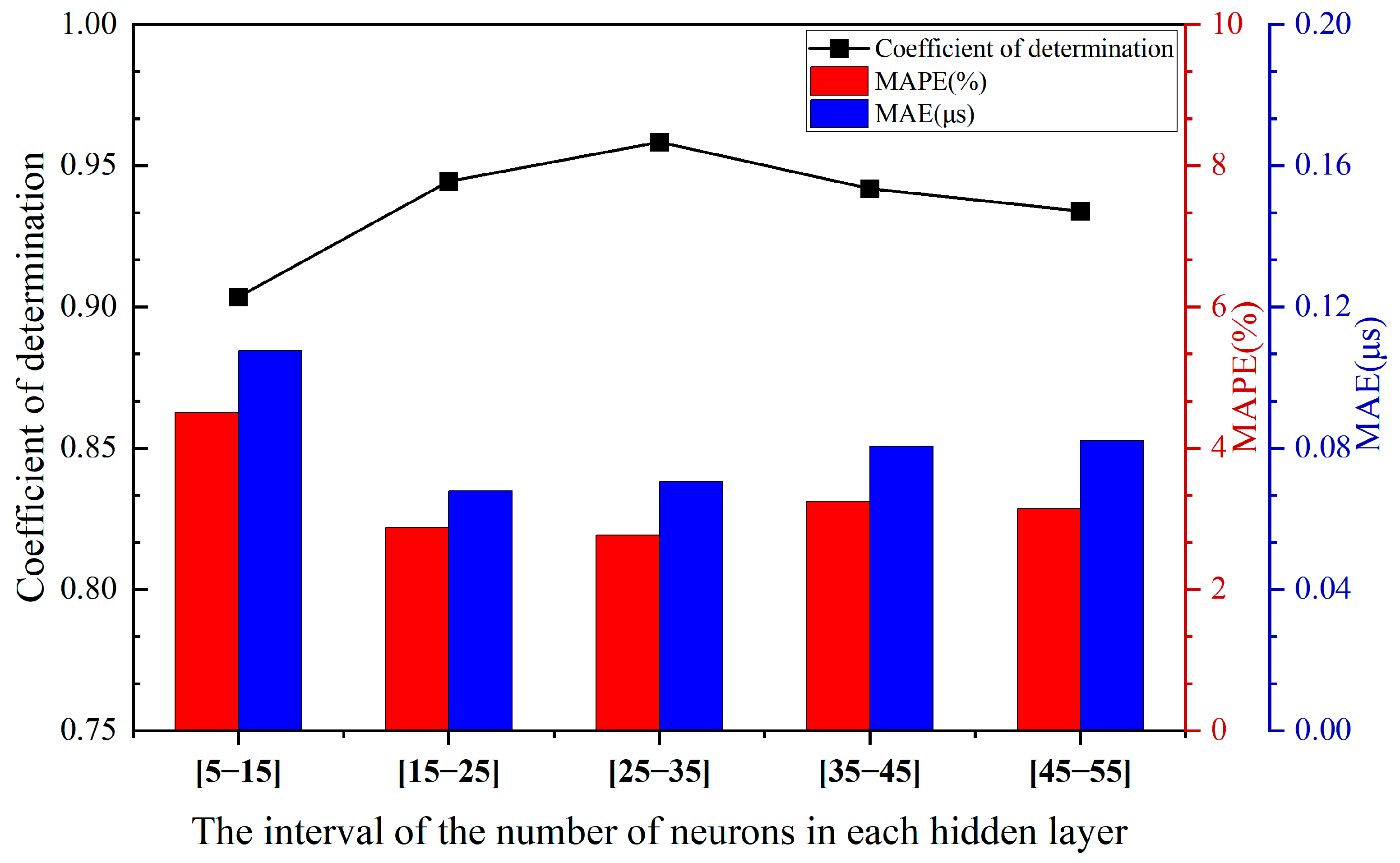
3.1.1. Determination of the Optimal Hidden Layer

In a BP neural network, the design of the hidden layer structure is one of the critical factors influencing the model’s performance. The appropriate configuration of layers and neurons not only affects the model’s approximation and learning capabilities but also determines its training efficiency and generalization ability. To construct an optimal network structure for predicting the ignition delay time of RP-3 aviation kerosene, this paper proposes two-hidden-layer and three-hidden-layer structures based on empirical formulas and practical fitting results. Furthermore, it systematically adjusts the number of neurons in the hidden layers to conduct an in-depth investigation into the hidden layer configuration for predicting the ignition delay time of RP-3.

In previous BP neural networks, the selection of the number of hidden layer nodes typically uses the following empirical formula:

$$\mathrm{h}={\displaystyle \frac{{\mathrm{n}}_{\mathrm{i}\mathrm{n}}+{\mathrm{n}}_{\mathrm{o}\mathrm{u}\mathrm{t}}}{2}}+\mathrm{C}$$

(19)

where ${\mathrm{n}}_{\mathrm{i}\mathrm{n}}$ is the number of input layer nodes, ${\mathrm{n}}_{\mathrm{o}\mathrm{u}\mathrm{t}}$ is the number of output layer nodes, and C is an empirical constant, usually ranging from 1 to 10. However, the number of hidden layer nodes selected based on the empirical formula is solely determined by the number of input and output layer nodes. In practice, the required number of nodes often exceeds the value suggested by the empirical formula. Therefore, for the multi-input variable ignition delay data analyzed in this study, the range of hidden layer nodes derived from the empirical formula is [5–15]. To explore a broader range, we extend the number of hidden layer nodes to [15–55]. Among the 50 possible node numbers within this extended range, the optimal hidden layer configuration is defined as the one achieving the maximum R² value on the test set. By randomly selecting the specified number of hidden layer nodes within the five subranges of [5–15], [15–25], [25–35], [35–45], and [45–55], two-hidden-layer and three-hidden-layer networks are constructed. The performance of these models within each subrange is evaluated using R², MAE, and MAPE metrics.

For the double- and triple-hidden-layer models, 30 repeated calculations were performed within the range of 5 to 20 neurons using the SGD algorithm. The results are presented in Figure 3 and Figure 4. All models shared the same initial learning rate and activation function. Figure 3 and Figure 4 correspond to the performance comparison of the double and triple hidden-layer structures, respectively, within the range of 5 to 20 neurons. These figures clearly illustrate the performance differences of neural network structures with varying numbers of hidden layers under different neuron configurations.

It can be observed from Figure 3 and Figure 4 as well as

Table 3. Training results across different hidden-layer configurations.

Hidden-Layer Structure	Range of the Hidden Layer	R2	MAPE (%)	MAE (μs)
two-hidden-layer structure	[5–15]	0.91099	5.23362	0.11951
	[15–25]	0.93781	3.57593	0.081
	[25–35]	0.90006	4.77065	0.1167
	[35–45]	0.94042	3.62867	0.08418
	[45–55]	0.92087	3.88182	0.08478
three-hidden-layer structure	[5–15]	0.90349	4.50252	0.10757
	[15–25]	0.94449	2.87703	0.0679
	[25–35]	0.95831	2.77153	0.07051
	[35–45]	0.9418	3.24754	0.08054
	[45–55]	0.9339	3.14394	0.08222

that the overall fitting performance of the three-hidden-layer structure is superior to that of the two-hidden-layer structure. Across the entire neuron range, the average coefficient of determination R² for the three-hidden-layer structure is consistently higher than that of the two-hidden-layer structure, particularly in the intervals [15–25], [25–35], [35–45], and [45–55], where it exceeds 0.93. Additionally, both the MAPE and MAE metrics are relatively low, with minimum values of 2.7715% and 0.0679, respectively, indicating that the three-hidden-layer structure offers greater advantages in terms of fitting and prediction accuracy. Although the two-hidden-layer model achieves a relatively high R² (approximately 0.94) in certain intervals (e.g., [35–45]), its error volatility across the hidden layer range is larger, and its stability is inferior to that of the three-hidden-layer structure.

When the number of hidden layer neurons is excessively small (e.g., [5–15]), the model experiences underfitting, leading to a low R² value and substantial errors. This confirms that for ignition delay data with multiple input variables, the number of hidden layer nodes determined by empirical formulas does not yield optimal fitting results. When the number of neurons is moderate (e.g., [15–35]), the model can effectively capture data characteristics while maintaining error control. In cases where the number of neurons is excessive (e.g., [45–55]), although training accuracy improves marginally, test errors slightly increase, indicating the onset of overfitting. Multiple training instances reveal that the error variation trends in the three-hidden-layer model on both the training and validation sets are consistent, demonstrating excellent generalization ability. Moreover, from the perspective of network stability, the performance fluctuations of the three-hidden-layer structure under different batch divisions are minimal, suggesting that this architecture is more robust.

Based on the above analysis, considering model fitting capability, error performance, training stability, and complexity balance, a three-hidden-layer architecture was ultimately selected. The number of neurons in each hidden layer was constrained within the range of [15–35], which was identified as the optimal structural range for this study. The ABC algorithm was then applied to perform optimization within this range.

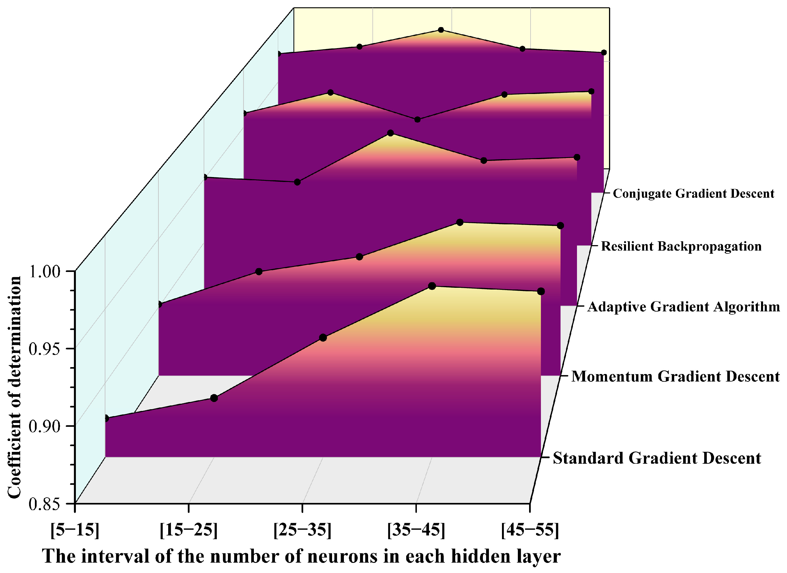
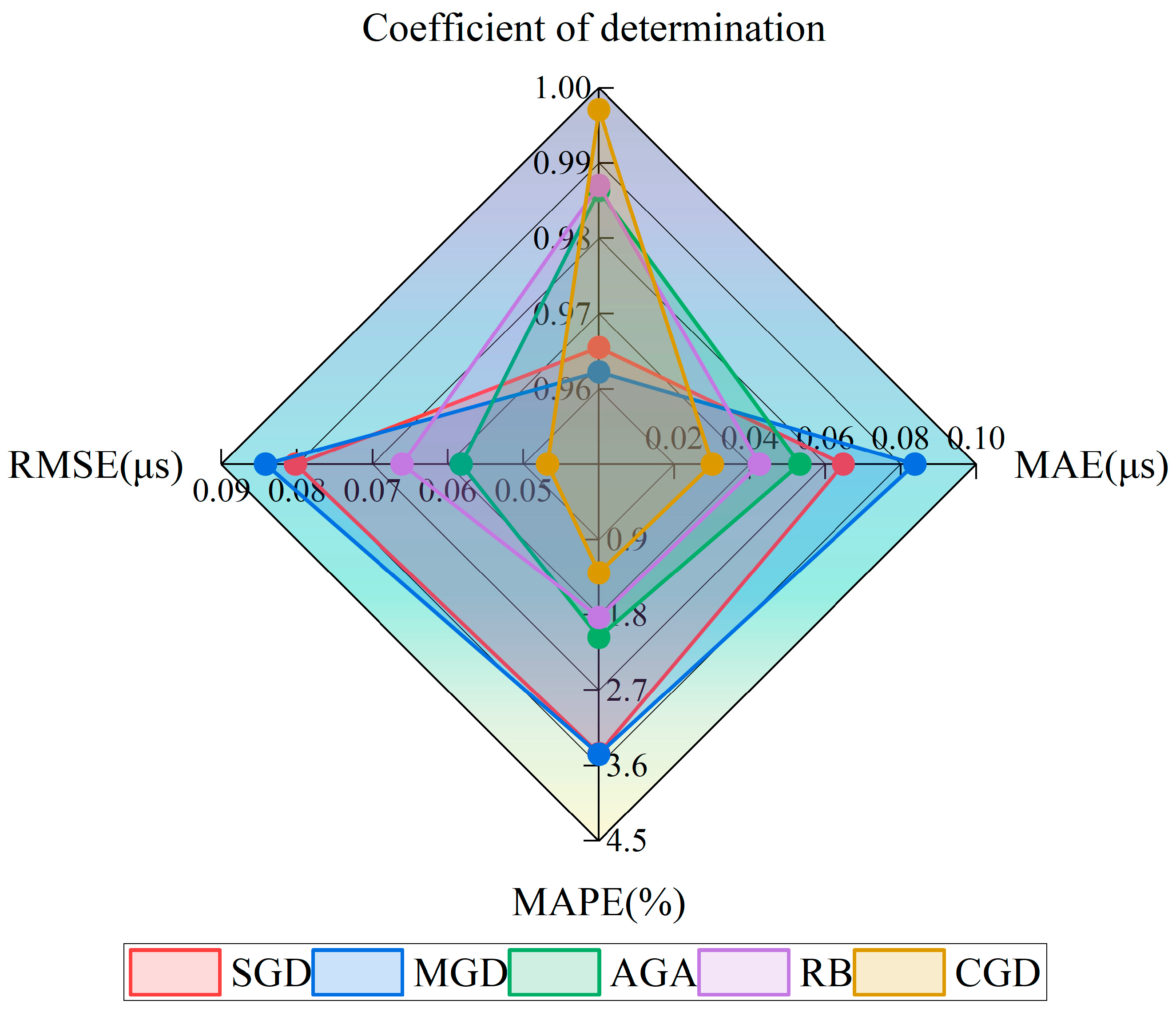
3.1.2. Neural Networks Founded on Diverse Gradient Descent Algorithms

To further enhance the prediction performance of the BP neural network for the ignition delay time of RP-3 aviation kerosene, this article introduces and compares five typical gradient optimization algorithms: SGD, MGD, AGA, RPROP, and CGD. By incorporating the interval variations in the number of neurons in the hidden layer, specifically [5–15], [15–25], [25–35], [35–45], and [45–55], multiple experiments were conducted. The prediction performance of each algorithm under different network configurations was evaluated using three metrics: R², mean absolute error (MAE), and mean absolute percentage error (MAPE). The results are presented in Figure 5, Figure 6 and Figure 7.

It can be observed from the above pictures that the CGD method demonstrates a markedly superior fitting capability across all neuron intervals. The R² value remains consistently above 0.98, reaching a peak of 0.99705 in the [25–35] interval, which is nearly indistinguishable from 1. In contrast, the R² value of the SGD method exhibits significant fluctuations, with the maximum deviation approaching 0.09, indicating its limited ability to fit complex nonlinear relationships. The RPROP algorithm and the AGA also perform well in most intervals; however, the R² value of the AGA slightly decreases in intervals with extremely small or large numbers of neurons. Furthermore, based on the MAE distribution results, the CGD method achieves the lowest error of 0.03 in the [15–25] interval, significantly outperforming other algorithms in terms of prediction accuracy and stability. The RPROP method shows comparable performance in the middle interval [15–25]. Conversely, the MAE of the SGD method exceeds 0.07 in all intervals, with noticeable fluctuations. Additionally, the CGD method exhibits the lowest MAPE in the [15–25] interval, approximately 1.2%, and maintains a MAPE below 2.5% across all intervals. By comparison, the MAPE of the SGD method surpasses 4% in some intervals, demonstrating its inferior performance. The trend in MAPE further corroborates the aforementioned conclusions. Overall, the CGD method clearly outperforms other optimization algorithms in terms of fitting accuracy and error control.

In the comparative experiment between the double-hidden-layer and triple-hidden-layer structures presented in Section 3.1, the triple-hidden-layer structure exhibited superior R² scores, smaller MAE, and lower MAPE values across most configurations. This indicates its stronger generalization capability and enhanced fitting performance. Furthermore, in conjunction with the results depicted in Figure 8, it is evident that the triple-hidden-layer structure performs exceptionally well within the [15–35] neuron range. Specifically, the CGD method achieves optimal overall performance within this range. To ascertain the ideal number of neurons for the model, this study identified the best-performing models corresponding to each gradient descent algorithm within the [15–35] neuron range during training and visualized these findings in Figure 8 for direct comparison. The radar chart reveals that the model with [21 17 19] neurons under the CGD algorithm excels across all five evaluation metrics, showcasing the smallest error contour. Consequently, the model featuring a triple-hidden-layer neuron distribution of [21 17 19], utilizing the CGD method and a random activation function strategy, was ultimately selected as the optimal network structure configuration for this study.

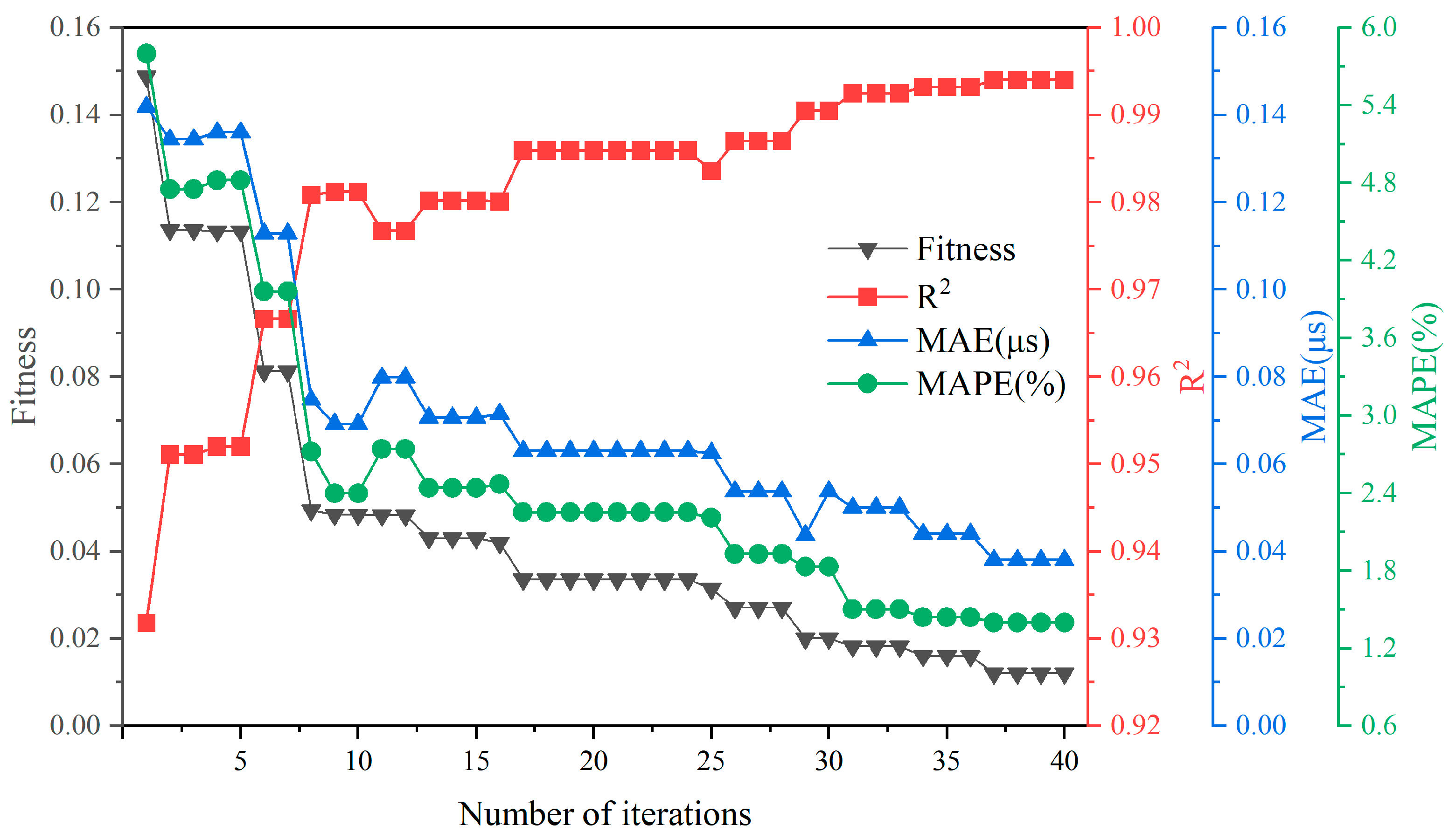
3.2. Optimization Using the Artificial Bee Colony Algorithm

To further enhance the prediction stability and generalization capability of the BP neural network under a fixed architecture, this study adopts the artificial bee colony (ABC) algorithm to globally optimize the network’s initial weights and biases. This is based on the previously determined three-hidden-layer structure with [21 17 19] neurons.

To suppress overfitting, an L2 regularization term (i.e., weight decay) is incorporated during training. This joint strategy improves both the robustness and reproducibility of the model. The ABC algorithm uses the regularized loss function on the validation set as the fitness metric, as defined in Equation (20):

$${\mathrm{Loss}}_{\mathrm{ABC}}={\mathrm{MSE}}_{\mathrm{val}}+\mathrm{\lambda }\sum _{\mathrm{i}=1}^{\mathrm{n}}{\mathrm{w}}_{\mathrm{i}}^2$$

(20)

where ${\mathrm{MSE}}_{\mathrm{val}}$ is the mean squared error on the validation set, ${\mathrm{w}}_{\mathrm{i}}$ represents all weight parameters, and λ is the regularization coefficient. The initial value of λ is set to 0.001, which has been empirically shown to effectively constrain weight magnitudes without excessively hindering the learning capability. Bias terms are excluded from regularization.

The network is still trained using the CGD method, but each candidate solution (i.e., a specific set of initialized parameters) is generated by the ABC algorithm. The iterative optimization process is illustrated in Figure 9.

The model’s predictive performance is illustrated in Figure 10. It is worth noting that under a single random data split, the metrics for CGD-BP in

Table 4. Comparison of training results between CGD-BP and CGD-ABC-BP neural networks.

Model Type	R2	MAE (μs)	MSE (μs2)	MAPE (%)
CGD-BP	0.997	0.03	0.006	1.2
CGD-ABC-BP	0.994	0.04	0.007	1.4

are slightly better than those for CGD-ABC-BP. This may be attributed to the use of random seeds during each train–validation–test split. If the data distribution is skewed, structurally similar samples may coincidentally fall into the validation set, leading to artificially improved performance for CGD-BP. In contrast, CGD-ABC-BP incorporates regularization, which sacrifices such extreme fitting in favor of better generalization.

However, considering 30 resampling trials, the CGD-ABC-BP model achieved significantly better performance than the CGD-BP model, with R² = 0.994 ± 0.001, MSE = 0.07 ± 0.01, MAE = 0.04 ± 0.015, and MAPE = 1.4 ± 0.05%, demonstrating the advantage of the ABC algorithm in global weight search and overall robustness.

Therefore, the CGD-ABC-BP model with a three-hidden-layer structure of [21, 17, 19] is selected as the optimal network configuration for this study.

3.3. Evaluation of Model Prediction Effect

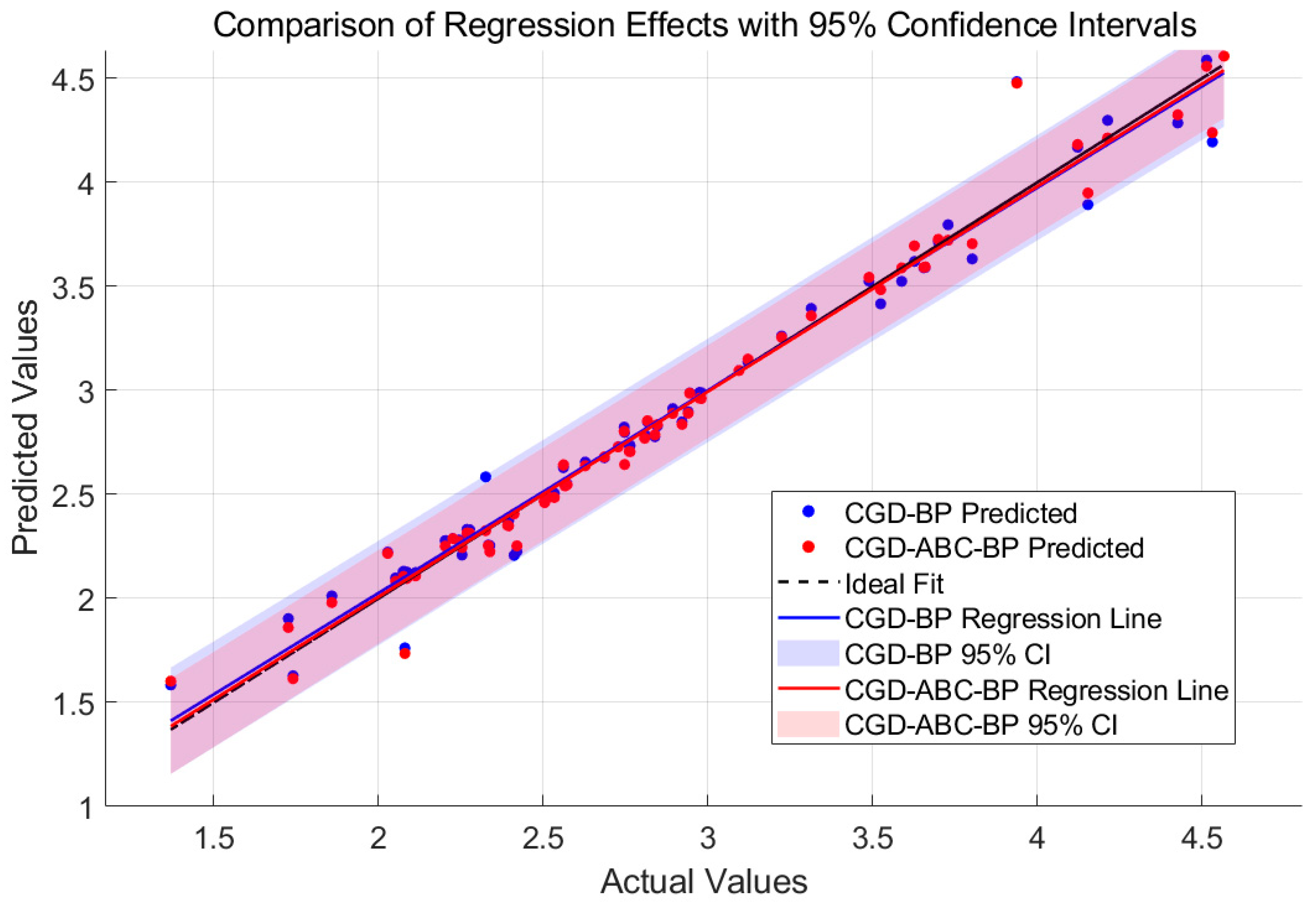
3.3.1. The Predictive Performance of the Model

It can be observed from Figure 11 that under the working condition of φ = 1.0, the overall trend in the prediction points closely matches the actual points across various pressure conditions. Specifically, under medium- and low-pressure conditions, the prediction points at 10 bar and 15 bar almost entirely overlap with the actual points, indicating the model’s high prediction accuracy and consistency in lower pressure ranges. However, under the high-pressure condition of 20 bar, some prediction points show slight deviations from the actual points, although the deviation is minimal and the overall trend remains consistent. This underscores the model’s reliability for IDT prediction under high-pressure conditions and further validates its excellent fitting capability across a wide range of pressures.

Further, in the image in which φ = 1.5 (Figure 12), the correlation between the predicted points and the actual points is significantly enhanced across all pressure conditions. The ignition delay time variation under different pressures is precisely captured by the predicted points, showing a stable distribution with minimal deviations. Within the pressure range of 10–20 bar, the predicted points exhibit excellent agreement with the experimental data. Notably, at pressures of 10 bar and 20 bar, the predicted points almost perfectly overlap with the actual points, indicating that the model achieves high fitting accuracy and demonstrates robust generalization performance in the medium equivalence ratio and high-pressure regime.

The reaction pathway of the fuel in a fuel-rich environment is highly complex. For the operating condition with φ = 2.0, the performance at various pressure points shows nuanced differences, as depicted in Figure 13. At 20 bar, the predicted values are closely aligned with the actual values. However, in the lower-pressure range, the predicted values exhibit a certain degree of systematic deviation, where they tend to be slightly higher or lower than the actual values. Despite this, the predicted values generally follow the variation trend in the actual values without significant deviation in the overall trend.

To further verify the model’s generalization ability on unseen data, an external test set comprising 70 ultra-low-pressure shock tube samples—sourced from the literature [29] and completely independent of the training process—was utilized. As illustrated in Figure 14, the vast majority of prediction points lie along the ideal line y = x and within the ±1σ confidence interval, indicating that the model maintains strong consistency and stability under varying conditions of temperature (1113–1600 K), pressure (1–5 bar), and equivalence ratio (0.5, 1.0, 1.5).

These results, as shown in Figure 14, comprehensively demonstrate that the CGD-ABC-BP model not only achieves excellent metrics during internal cross-validation but also sustains high prediction accuracy on entirely new datasets. This provides robust support for its applicability in practical engineering deployment.

In summary, as illustrated in Figure 11, Figure 12, Figure 13 and Figure 14, the BP neural network model demonstrates excellent prediction consistency under most pressure conditions, particularly exhibiting robust performance in medium and low-pressure environments. At a few specific points under certain operating conditions, the prediction error marginally increases, indicating that there is still potential for improving the model’s accuracy. The model prediction outcomes from this study provide a solid foundation for further refining model training and optimizing sample distribution.

3.3.2. Importance and Sensitivity Analysis

To systematically investigate the effects of each input variable on the ignition delay time of RP-3 aviation fuel across different temperature ranges, this study conducted feature importance analysis and sensitivity analysis. All results were statistically analyzed separately for the three temperature regions: low temperature (600–900 K), NTC (900–1100 K), and high temperature (1100–1500 K).

Permutation importance analysis was employed to assess the relative contribution of each input variable. This method involves randomly shuffling the values of a specific input variable in the validation set, and then recalculating the model’s performance metrics (R², MAPE, MAE) on the perturbed dataset. The decrease in model performance indicates the importance of the variable being shuffled.

This process was repeated N = 50 times for each input variable, and the average performance change was used to quantify its importance to the prediction output. The importance score for a given variable is defined as follows:

$$\mathrm{I}={\displaystyle \frac{{\mathrm{M}}_{\mathrm{perm}}-{\mathrm{M}}_{\mathrm{orig}}}{{\mathrm{M}}_{\mathrm{orig}}}}$$

(21)

where ${\mathrm{M}}_{\mathrm{perm}}$ represents the model performance after shuffling the variable, and ${\mathrm{M}}_{\mathrm{orig}}$ is the performance on the original validation set.

Sensitivity analysis was conducted using a baseline point gradient analysis method. Specifically, 20 representative sample points were randomly selected from each temperature region, resulting in a total of 60 points. For each input feature at every selected point, five perturbed values were generated through linear interpolation within a ±50% range, while keeping all other variables constant. The corresponding outputs were predicted using the trained model, and a first-order linear regression was fitted to evaluate the relationship between the input perturbations and the output response:

$$\mathrm{y}={\mathrm{a}}_{\mathrm{j}}{\mathrm{x}}_{\mathrm{j}}+\mathrm{b}$$

(22)

where the slope ${\mathrm{a}}_{\mathrm{j}}$ is defined as the sensitivity coefficient of the corresponding input feature. The average sensitivity coefficient across all representative points in a given temperature region is taken as the final sensitivity value for that variable in that region:

$${\mathrm{S}}_{\mathrm{j}}={\displaystyle \frac{1}{\mathrm{N}}}\sum _{\mathrm{i}=1}^{\mathrm{N}}{\mathrm{a}}_{\mathrm{j}}^{\left(\mathrm{i}\right)}$$

(23)

The sign of the sensitivity coefficient indicates the direction of influence (i.e., whether the input change leads to an increase or decrease in the output), while the absolute value reflects the strength of that influence. This analysis framework is adapted from the local gradient sensitivity analysis procedures described by Zhao et al. [28] and Zhang et al. [27], ensuring both physical interpretability and statistical robustness.

From the importance analysis results presented in Figure 15, it is evident that in the low-temperature region, the molar fractions of the oxidant (0.3285) and the diluent (0.2757) exhibit the highest significance, surpassing other factors. This indicates that the molar fractions of the oxidant and diluent have a more pronounced effect on ignition delay time in the low-temperature region. Following these are the molar fraction of the fuel (0.1193) and the pressure of the mixture gas (0.1196), whereas the temperature (0.0569) has a relatively minor influence. In the medium-temperature region, the importance of the molar fractions of the oxidant and diluent decreases slightly to 0.1671 and 0.1193, respectively. Conversely, the importance of the molar fraction of the fuel and the pressure of the mixture gas increases, and the importance of the ignition temperature rises significantly to 0.2195. In the high-temperature region, the importance of the ignition temperature further increases to 0.5057, while the significance of other factors diminishes, suggesting that at high temperatures, the ignition temperature plays a decisive role in determining the combustion reaction rate.

From the results of the sensitivity analysis presented in Figure 16, the ignition temperature exhibits pronounced negative sensitivity across all temperature regions (low-temperature region: −60.558, NTC region: −80.744, high-temperature region: −201.86). This indicates that an increase in temperature significantly reduces the ignition delay time, aligning with the principles of combustion kinetics. The diluent fraction also demonstrates negative sensitivity, with higher sensitivity observed in the NTC region (−100.38) and even greater sensitivity in the low-temperature region, suggesting that an increase in diluent concentration accelerates the reaction process. The sensitivity values of the mixture gas pressure are generally small but exhibit a negative trend, implying that increased pressure facilitates a reduction in ignition delay time, consistent with the model’s predictive capability discussed in Section 3.3.1. Both the fuel mole fraction and oxidant mole fraction display positive sensitivity, indicating that increases in these fractions tend to extend the ignition delay time, particularly in the high-temperature region, where the fuel mole fraction reaches its maximum sensitivity value (59.078).

To visually display the data sensitivity and importance in the low-temperature region, the NTC region, and the high-temperature region, we plotted the histogram as shown in Figure 17, Figure 18 and Figure 19 after taking the absolute value of the sensitivity coefficient and the importance coefficient.

In recent years, numerous experimental and kinetic studies have systematically revealed the dominant reaction pathways of RP-3 fuel across different temperature regimes and their impacts on macroscopic ignition delay time (IDT). By comparing the machine learning results from this study (Figure 11, Figure 12 and Figure 13) with these well-established physical trends, the physical reliability of the proposed model can be validated.

In the low-temperature region (T < 900 K), although the importance score of temperature was evaluated at 0.0569, the model still yielded a significantly negative sensitivity of −60.558, consistent with the conclusions of Liu et al. [30], who observed accelerated IDT reduction with increasing temperature during low-temperature oxidation and chain-branching experiments. The rankings and directional signs of diluent and oxidizer mole fractions also aligned with the experimental observations by Chen et al. [29] under ultra-low-pressure conditions.

In the negative temperature coefficient (NTC) region (≈900–1100 K), temperature showed extreme sensitivity. The model reported a sensitivity of −80.7, which matches the mechanistic explanation provided by Mao et al. [9] involving the competition between β-dehydrogenation and chain-branching pathways in combined compression machine and shock tube experiments. Furthermore, the model captured a high negative sensitivity of −100.4 for the diluent fraction, consistent with its experimentally verified role in suppressing free radical concentrations.

In the high-temperature region (T > 1100 K), the model identified temperature as the overwhelmingly dominant factor, with an importance score of 0.5057 and sensitivity of −201.9. This observation aligns well with the high-temperature Arrhenius-controlled regime characterized by Zhang et al. [33] in shock tube experiments.

In summary, the CGD-ABC-BP model successfully captured the dominant controlling factors and their directional effects across all three temperature regions. The quantitative differences in variable weights can primarily be attributed to variations in input value distributions and statistical measures, rather than any conflict with underlying chemical mechanisms. This comparative analysis strongly supports the physical consistency of the model and suggests that further expansion of the T–P–φ space coverage will enhance the representativeness of the resulting importance and sensitivity rankings.

4. Discussion

This study focuses on the prediction of ignition delay time (IDT) for RP-3 aviation kerosene and proposes a CGD-ABC-BP neural network model. A multi-stage hybrid optimization strategy was adopted to enhance model performance. The main conclusions are as follows:

• Within a five-input, one-output BP neural network framework, a multi-stage optimization model was developed by integrating randomized initialization, conjugate gradient descent (CGD), the artificial bee colony (ABC) algorithm, and L2 regularization. Based on 30 resampling trials, the model achieved average performance metrics of R² = 0.994 ± 0.001, MAE = 0.04 ± 0.015, MAPE = 1.4 ± 0.05%, and RMSE = 0.07 ± 0.01, demonstrating excellent fitting capability on internal data and structural stability.
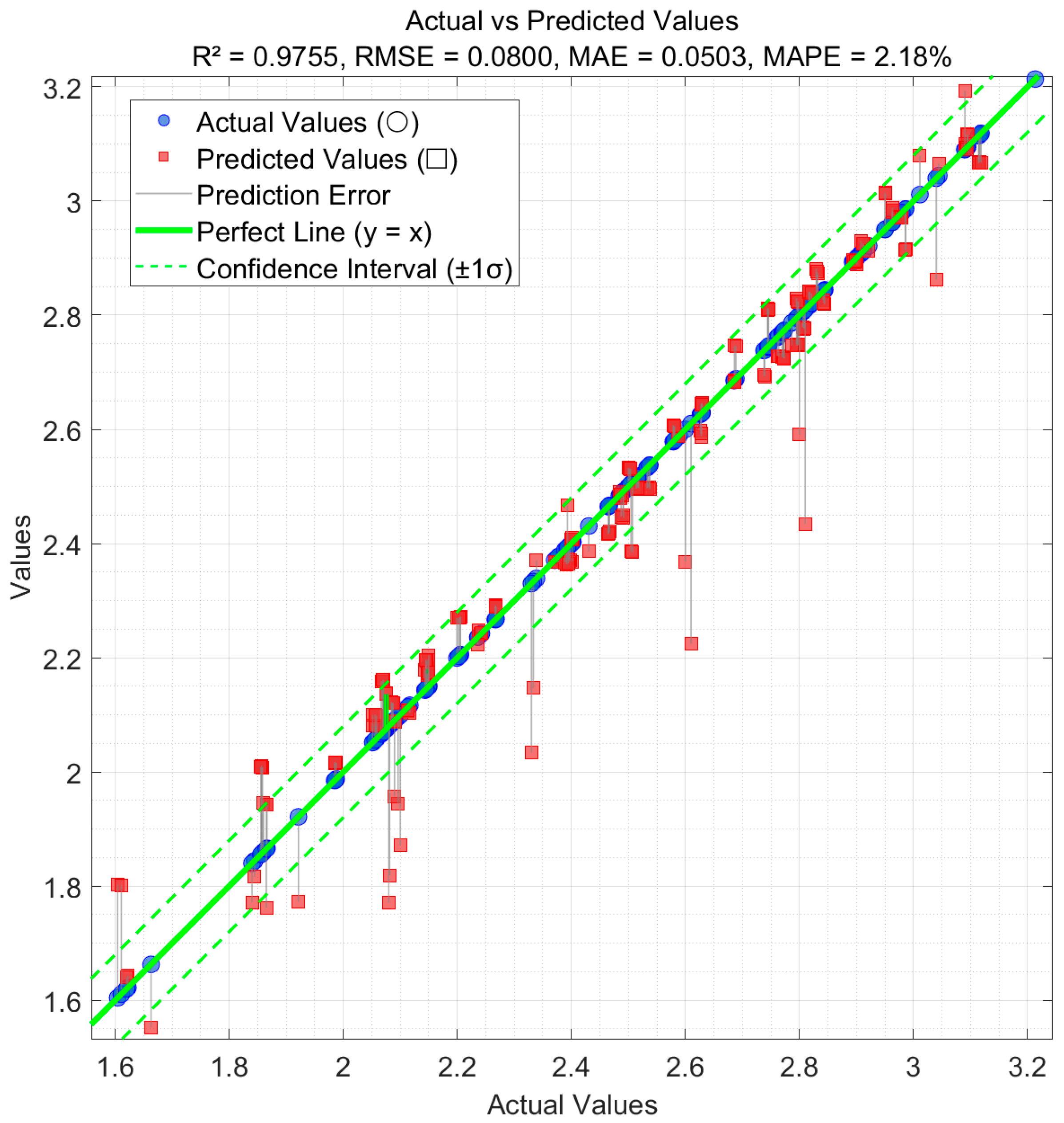
• Under various equivalence ratios (φ = 1.0, 1.5, 2.0) and pressure conditions (10–20 bar), the prediction outcomes exhibit high consistency with the experimental results. Notably, in scenarios with moderate equivalence ratios and low-to-medium pressure levels, the predicted points were almost perfectly aligned with the actual measurements. These results highlight the model’s good generalization and robustness in predicting the ignition delay time of RP-3 aviation kerosene. On a completely independent external test set, the model still achieved high accuracy with R² = 0.9755 and MAPE = 2.18%, further confirming its generalization capability and engineering feasibility. However, its cross-fuel applicability and consistency across different experimental setups require further validation using larger-scale, multi-source datasets.
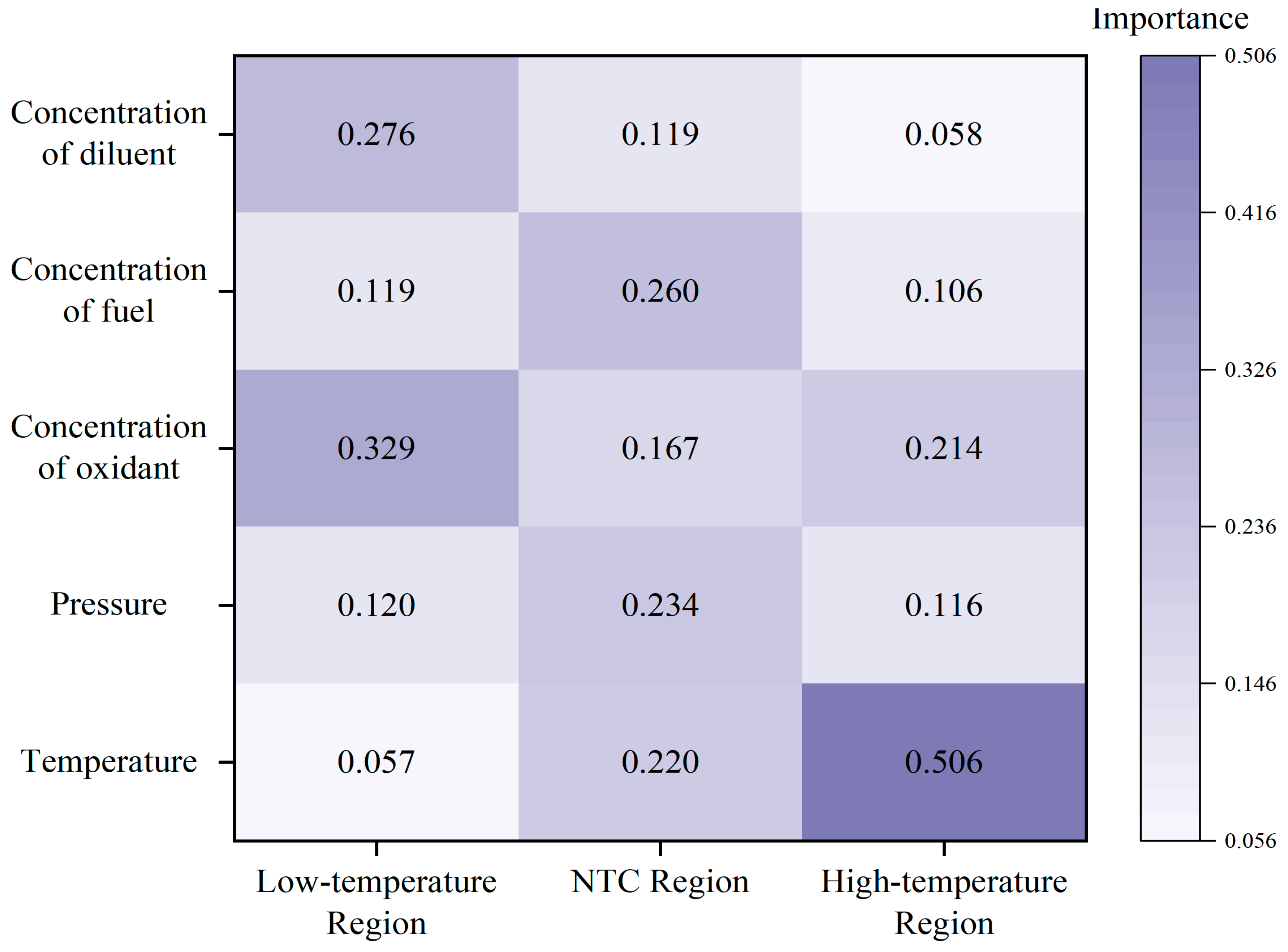
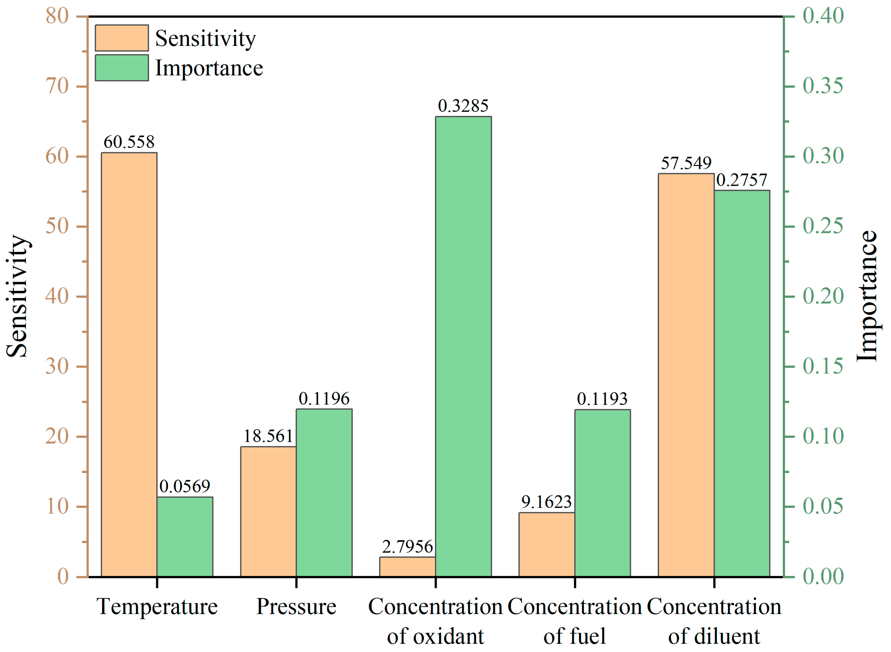
• In the low-temperature region, the diluent mole fraction exhibited an importance score of 0.2757 and a sensitivity of −57.549, while temperature showed a higher sensitivity (−60.558) but lower importance (0.0569). In the NTC region, temperature had an importance of 0.2195 and a sensitivity of −145.6, while the diluent displayed the highest sensitivity (−140.5). In the high-temperature region, temperature dominated with an importance of 0.5057 and a sensitivity of −201.86. These trends are consistent with well-established combustion kinetic mechanisms, indicating that the model possesses a degree of physical interpretability.
• The current model relies on five macroscopic input features and does not incorporate additional variables. Due to the scarcity of experimental data in extremely fuel-rich (φ > 2.0) and ultra-high-pressure (p > 20 bar) conditions, model extrapolation in these regimes carries a degree of uncertainty. Moreover, the model is specifically trained on RP-3 fuel, and its applicability to alternative fuels or multi-component mixtures remains unverified.
• Future work will focus on integrating the current framework with other machine learning techniques, incorporating input perturbation analysis and explainability tools such as SHAP and LIME, and extending its generalizability through multi-fuel transfer learning strategies.

References

1. Zeng, W.; Zou, C.; Yan, T.; Lin, Q.; Dai, L.; Liu, J.; Song, Y. High-temperature ignition of ammonia/methyl isopropyl ketone: A shock tube experiment and a kinetic model. Combust. Flame 2025, 276, 114004. [Google Scholar] [CrossRef]
2. Dai, L.; Liu, J.; Zou, C.; Lin, Q.; Jiang, T.; Peng, C. Shock tube experiments and numerical study on ignition delay times of ammonia/oxymethylene ether-2 (OME2) mixtures. Combust. Flame 2024, 270, 113783. [Google Scholar] [CrossRef]
3. Lin, Q.; Zou, C.; Dai, L. High temperature ignition of ammonia/di-isopropyl ketone: A detailed kinetic model and a shock tube experiment. Combust. Flame 2023, 251, 112692. [Google Scholar] [CrossRef]
4. Qu, Y.; Zou, C.; Xia, W.; Lin, Q.; Yang, J.; Lu, L.; Yu, Y. Shock tube experiments and numerical study on ignition delay times of ethane in super lean and ultra-lean combustion. Combust. Flame 2022, 246, 112462. [Google Scholar] [CrossRef]
5. Reyes, M.; Tinaut, F.V.; Andrés, C.; Pérez, A. A method to determine ignition delay times for Diesel surrogate fuels from combustion in a constant volume bomb: Inverse Livengood–Wu method. Fuel 2012, 102, 289–298. [Google Scholar] [CrossRef]
6. Wu, Y.; Liu, Y.; Tang, C.; Huang, Z. Ignition delay times measurement and kinetic modeling studies of 1-heptene, 2-heptene and n-heptane at low to intermediate temperatures by using a rapid compression machine. Combust. Flame 2018, 197, 30–40. [Google Scholar] [CrossRef]
7. De Toni, A.R.; Werler, M.; Hartmann, R.M.; Cancino, L.; Schießl, R.; Fikri, M.; Schulz, C.; Oliveira, A.; Oliveira, E.; Rocha, M. Ignition delay times of Jet A-1 fuel: Measurements in a high-pressure shock tube and a rapid compression machine. Proc. Combust. Inst. 2017, 36, 3695–3703. [Google Scholar] [CrossRef]
8. Ramalingam, A.; Fenard, Y.; Heufer, A. Ignition delay time and species measurement in a rapid compression machine: A case study on high-pressure oxidation of propane. Combust. Flame 2020, 211, 392–405. [Google Scholar] [CrossRef]
9. Mao, Y.; Yu, L.; Wu, Z.; Tao, W.; Wang, S.; Ruan, C.; Zhu, L.; Lu, X. Experimental and kinetic modeling study of ignition characteristics of RP-3 kerosene over low-to-high temperature ranges in a heated rapid compression machine and a heated shock tube. Combust. Flame 2019, 203, 157–169. [Google Scholar] [CrossRef]
10. Schulz, C.; Sick, V. Tracer-LIF diagnostics: Quantitative measurement of fuel concentration, temperature and fuel/air ratio in practical combustion systems. Prog. Energy Combust. Sci. 2005, 31, 75–121. [Google Scholar] [CrossRef]
11. Shah, Z.A.; Marseglia, G.; De Giorgi, M.G. Predictive models of laminar flame speed in NH3/H2/O3/air mixtures using multi-gene genetic programming under varied fuelling conditions. Fuel 2024, 368, 131652. [Google Scholar] [CrossRef]
12. Wang, Y.; Zhou, X.; Liu, L. Study on the mechanism of the ignition process of ammonia/hydrogen mixture under high-pressure direct-injection engine conditions. Int. J. Hydrogen Energy 2021, 46, 38871–38886. [Google Scholar] [CrossRef]
13. Yamada, S.; Shimokuri, D.; Shy, S.; Yatsufusa, T.; Shinji, Y.; Chen, Y.-R.; Liao, Y.-C.; Endo, T.; Nou, Y.; Saito, F.; et al. Measurements and simulations of ignition delay times and laminar flame speeds of nonane isomers. Combust. Flame 2021, 227, 283–295. [Google Scholar] [CrossRef]
14. Mao, G.; Zhao, C.; Yu, H. Optimization of ammonia-dimethyl ether mechanisms for HCCI engines using reduced mechanisms and response surface methodology. Int. J. Hydrogen Energy 2025, 100, 267–283. [Google Scholar] [CrossRef]
15. Song, T.; Wang, C.; Wen, M.; Liu, H.; Yao, M. Combustion mechanism study of ammonia/n-dodecane/n-heptane/EHN blended fuel. Appl. Energy Combust. Sci. 2024, 17, 100241. [Google Scholar] [CrossRef]
16. Gong, Z.; Feng, L.; Wei, L.; Qu, W.; Li, L. Shock tube and kinetic study on ignition characteristics of lean methane/n-heptane mixtures at low and elevated pressures. Energy 2020, 197, 117242. [Google Scholar] [CrossRef]
17. Kelly, M.; Bourque, G.; Hase, M.; Dooley, S. Machine learned compact kinetic model for liquid fuel combustion. Combust. Flame 2025, 272, 113876. [Google Scholar] [CrossRef]
18. Zhang, H.; Hu, Y.; Liu, W.; Zhao, C.; Fan, W. Update of the present decomposition mechanisms of ammonia: A combined ReaxFF, DFT and chemkin study. Int. J. Hydrogen Energy 2024, 90, 557–567. [Google Scholar] [CrossRef]
19. Gong, Z.; Feng, L.; Li, L.; Qu, W.; Wei, L. Shock tube and kinetic study on ignition characteristics of methane/n-hexadecane mixtures. Energy 2020, 201, 117609. [Google Scholar] [CrossRef]
20. Wu, Y.; Li, Y.; Zhang, L. Data-driven modeling of ignition delay time using artificial neural networks. Energy 2020, 193, 116726. [Google Scholar]
21. Liu, Y.; Chen, Y. Application of neural network in combustion characteristics prediction of alternative aviation fuels. Fuel 2021, 294, 120576. [Google Scholar]
22. Wang, H.; Wang, Z.; Zhang, Y. Prediction of ignition delay times of surrogate jet fuels using machine learning methods. Fuel 2022, 308, 122048. [Google Scholar]
23. Zhang, C.; Lin, Y. Ignition delay prediction using deep learning with convolutional neural networks. Combust. Theory Model. 2022, 26, 135–150. [Google Scholar]
24. Patel, R.; Saxena, P. Sequence modeling of ignition delay using LSTM networks for real-time combustion diagnostics. Appl. Energy 2023, 345, 121042. [Google Scholar]
25. Cui, Y.; Liu, H.; Wang, Q.; Zheng, Z.; Wang, H.; Yue, Z.; Ming, Z.; Wen, M.; Feng, L.; Yao, M. Investigation on the ignition delay prediction model of multi-component surrogates based on back propagation (BP) neural network. Combust. Flame 2022, 237, 111852. [Google Scholar] [CrossRef]
26. Ji, W.; Su, X.; Pang, B.; Li, Y.; Ren, Z.; Deng, S. SGD-based optimization in modeling combustion kinetics: Case studies in tuning mechanistic and hybrid kinetic models. Fuel 2022, 324, 124560. [Google Scholar] [CrossRef]
27. Zhang, L.; Ma, Y.; Li, S. Improving generalization of neural network-based ignition delay prediction using transfer learning and data augmentation. Combust. Flame 2020, 215, 392–401. [Google Scholar]
28. Zhao, Y.; Xu, M. Feature sensitivity and interpretability analysis of neural network predictions in combustion systems. Fuel 2022, 314, 123089. [Google Scholar]
29. Chen, B.H.; Liu, J.Z.; Yao, F.; He, Y.; Yang, W.J. Ignition delay characteristics of RP-3 under ultra-low pressure (0.01–0.1 MPa). Combust. Flame 2019, 210, 126–133. [Google Scholar] [CrossRef]
30. Liu, J.; Hu, E.; Yin, G.; Huang, Z.; Zeng, W. An experimental and kinetic modeling study on the low-temperature oxidation, ignition delay time, and laminar flame speed of a surrogate fuel for RP-3 kerosene. Combust. Flame 2022, 237, 111821. [Google Scholar] [CrossRef]
31. Liu, J.; Hu, E.; Zeng, W.; Zheng, W. A new surrogate fuel for emulating the physical and chemical properties of RP-3 kerosene. Fuel 2020, 259, 116210. [Google Scholar] [CrossRef]
32. Yang, Z.Y.; Zeng, P.; Wang, B.Y.; Jia, W.; Xia, Z.-X.; Liang, J.; Wang, Q.-D. Ignition characteristics of an alternative kerosene from direct coal liquefaction and its blends with conventional RP-3 jet fuel. Fuel 2021, 291, 120258. [Google Scholar] [CrossRef]
33. Zhang, C.; Li, B.; Rao, F.; Li, P.; Li, X. A shock tube study of the autoignition characteristics of RP-3 jet fuel. Proc. Combust. Inst. 2015, 35, 3151–3158. [Google Scholar] [CrossRef]
Figure 1. Schematic representation of the BP neural network architecture.
Energies 18 03037 g001
Figure 2. Flowchart of the artificial bee colony (ABC) algorithm.
Energies 18 03037 g002
Figure 3. Performance comparison of two-hidden-layer structures across different neuron intervals.
Energies 18 03037 g003
Figure 4. Performance comparison of the three-hidden-layer structure across different neuron intervals.
Energies 18 03037 g004
Figure 5. MAE values obtained from various gradient descent algorithms.
Energies 18 03037 g005
Figure 6. R2 values obtained from various gradient descent algorithms.
Energies 18 03037 g006
Figure 7. MAPE values obtained from various gradient descent algorithms.
Energies 18 03037 g007
Figure 8. Comparison of evaluation indicators of five different gradient descent algorithms.
Energies 18 03037 g008
Figure 9. Optimization process of the ABC algorithm.
Energies 18 03037 g009
Figure 10. Comparison of regression lines between CGD-BP and CGD-ABC-BP models.
Energies 18 03037 g010
Figure 11. Data prediction when the equivalence ratio is 1 and the pressures are 20 bar, 15 bar, and 10 bar, respectively. Data adopted from Mao et al. [9].
Energies 18 03037 g011
Figure 12. Data prediction when the equivalence ratio is 1.5 and the pressures are 20 bar, 15 bar, and 10 bar, respectively. Data adopted from Mao et al. [9].
Energies 18 03037 g012
Figure 13. Data prediction when the equivalence ratio is 2 and the pressures are 20 bar and 10 bar, respectively. Data adopted from Mao et al. [9].
Energies 18 03037 g013
Figure 14. Prediction performance of the CGD-ABC-BP model on the external test set.
Energies 18 03037 g014
Figure 15. Analysis of the importance of data.
Energies 18 03037 g015
Figure 16. Analysis of the sensitivity of data.
Energies 18 03037 g016
Figure 17. The distribution of sensitivity and importance in the low-temperature region.
Energies 18 03037 g017
Figure 18. The distribution of sensitivity and importance in the NTC region.
Energies 18 03037 g018
Figure 19. The distribution of sensitivity and importance in the high-temperature region.
Energies 18 03037 g019