The Impact of Terminal-Voltage Control on the Equilibrium Points and Small-Signal Stability of GFL-VSC Systems

Abstract

Weak grid stability is crucial for grid-following voltage source converter (GFL-VSC) systems. Current studies primarily focus on the interaction analyses between active-power loops, whereas the influence of reactive-power loops remains unclear. To address this problem, this study focuses on terminal-voltage control (TVC) and analyzes its impact on equilibrium points (EPs) and small-signal stability by varying the TVC response speed, including three different cases: considering TVC dynamics, considering TVC rapid responses, and considering TVC slow responses. Firstly, the models of the GFL-VSC system under different scenarios are established and compared. In the EP analysis, for both TVC dynamics and TVC rapid responses, the EP of an active current remains constant and it becomes unstable in a weak grid, whereas for TVC slow responses, the EP undergoes trans-critical bifurcation; specifically, the other EP becomes stable after this bifurcation. Further, in the small-signal stability analysis, three equivalent Heffron–Phillips models based on the phase-locked loop synchronization dynamics with additional synchronization and damping coefficients are constructed and studied. By these systematical studies, the impacts of different TVC response speeds are clarified and summarized, and these analytical results are well supported by MATLAB/Simulink simulations and hardware-in-the-loop experiments.

1. Introduction

Under the carbon peaking and carbon neutrality (i.e., the so-called dual-carbon target), the installed capacity of clean energy in China by the end of 2024 reached 1.889 billion kilowatts, marking a 25% year-on-year increase and accounting for 56% of the total installed capacity. Among them, the cumulative installed capacities of wind power and photovoltaic (PV) power are 521 million and 887 million kilowatts, respectively [1]. The large-scale integration of renewable energy, such as wind and PV power, is realized primarily by power electronic devices based on voltage source converters (VSCs). This has become an utmost characteristics of the new-generation power system [2,3]. The widespread emergence of grid-following (GFL)-VSC inevitably leads to new stability problems, due to its inherent properties, such as weak damping and low inertia [4,5,6]. These issues become particularly pronounced under weak grids and may be attributed to the interactions among the control components of devices [7,8].

The control structure of GFL-VSCs can be typically divided into three main components: synchronization control, active-power control, and reactive-voltage control. For the synchronization control, the phase-locked loop (PLL) is the most widely adopted. The active power input is regulated by controlling the voltage across the DC capacitor. For reactive-voltage control, there are generally three approaches [9,10]: terminal-voltage control (TVC), reactive-power control, and cascaded reactive-power and terminal-voltage control. In this paper, without losing generality, the TVC will be selected to investigate its impact on the equilibrium points (EPs) and small-signal stability of the GFL-VSC system.

The existence of EPs serves as a prerequisite for small-signal or large-signal (transient) stability, and hence it is very important. Refs. [11,12,13,14,15] focus on the second-order PLL control and investigate the impact of the ratio between active and reactive currents’ injection on the existence of EPs during the low-voltage ride-throughs. The optimal injection condition is also obtained. On the other hand, refs. [16,17,18] concentrate on the second-order DC-voltage control (DVC) loop, explore the influence of reactive current injection, and obtain the static stability range. The EP of the GFL-VSC system within the DC voltage time scale is studied, and its disappearance is found due to a generalized saddle-node bifurcation [19]. However, in all these studies, the role of TVC is not paid enough attention. Therefore, to fill this gap, this paper will systematically study all possibilities for different response speeds of TVC and analyze the changes in EP induced by these responses.

In contrast, small-signal stability of the GFL-VSC system has been widely investigated. By completely ignoring TVC dynamics, ref. [20] proposes the concept of a static synchronous generator and shows the similarity between VSC and the synchronous generator. It obtains the equivalent parameters such as equivalent synchronization, damping, and inertia, which are related to DVC. Oppositely, ref. [21] neglects TVC dynamics and employs the bandwidth separation method to study the interaction between PLL and DVC. By constructing an equivalent Heffron–Phillips model, it is clearly demonstrated that the system becomes unstable under a weak grid. Further, ref. [22] analyzes the GFL-VSC system under two different conditions: with TVC and without TVC. It finds that without TVC, the system exhibits monotonic instability under a weak grid, consistent with that in [21], whereas when TVC is incorporated, its integral gain introduces additional negative damping, which leads to oscillatory instability. It should be noted that all these studies obtain their stability conditions based on the fixed EP. Oppositely, this paper will highlight a closer relation between EPs and small-signal stability, and provide a systematical stability analysis based on the variations of EPs under different TVC response speeds.

The remaining of this paper is organized as follows: Section 2 introduces the topology and controls of the GFL-VSC system and establishes a nonlinear model. Section 3 analyzes the EPs and their existence conditions under different response speeds of TVC. Based on these EPs, Section 4 constructs equivalent Heffron–Phillips models and derives the synchronization and damping coefficients for all cases by using the complex torque method. Small-signal stability is analyzed based on the total negative damping coefficient. In Section 5, these analytical results are validated by root locus analysis and time-domain simulations. Further, Section 6 provides hardware-in-the-loop experiment results. Finally, the conclusions are outlined in Section 7.

2. Description of GFL-VSC-Based Power System

2.1. System Topology

The topology and control structure of the GFL-VSC system are illustrated in Figure 1. The GFL-VSC is connected to the infinite bus $U_g$ via filter inductance $L_f$ and line inductance $L_g$. The amplitude and phase of the terminal voltage are denoted as $U_t$ and ${\theta }_t$, respectively, while I represents the current flowing on the line. The control structure consists of four main components, including PLL, DVC, TVC, and the alternating current control (ACC) loop. The PLL establishes a $dq$ rotating reference frame to facilitate synchronization with the grid. DVC and TVC serve as the two voltage control outer loops, responsible for regulating DC voltage $U_{dc}$ and terminal voltage $U_t$, respectively. These controls ensure that $U_{dc}$ and $U_t$ are within allowable ranges to maintain system stability. Simultaneously, they generate the reference currents $i_{dref}$ and $i_{qref}$, which serve as inputs to the ACC inner loop. By the proportional-integral (PI) control applied to the $dq$-axis components of the output current ($i_d$ and $i_q$), the $dq$-axis components of the output voltage E (i.e., $e_d$ and $e_q$) are obtained.

The relationship between the $dq$ rotating reference frame and the $xy$ synchronous reference frame is illustrated in Figure 2. The $dq$ reference frame rotates at a varying angular speed ${\omega }_{pll}$, while the $xy$ synchronous reference frame rotates at a constant speed ${\omega }_0$. The grid voltage $U_g$ is assumed to lie on the x-axis by default. The angle between $U_t$ and the x-axis is denoted as ${\theta }_t$, and the angle between the d-axis and the x-axis is denoted as ${\phi }_{pll}$. For the steady state, the output phase of PLL equals the terminal voltage phase, i.e., ${\phi }_{pll}$ = ${\theta }_t$.

2.2. Nonlinear Modeling of GFL-VSC System

Our previous study [23] has proposed a comprehensive nineth-order model for the GFL-VSC system, as shown in Figure 1, which includes the PLL synchronization loop, DVC, TVC, ACC, and line dynamics. The specific nonlinear state equations can be established as follows:

$$\left\{\begin{array}{c}{\dot{\phi }}_{pll}={\omega }_{pll}\hfill \\ {\dot{\omega }}_{pll}=k_{p1}{\dot{u}}_{tq}+k_{i1}{u}_{tq}\hfill \\ {\dot{U}}_{dc}=(P_{in}-P_e)/C{U}_{dc}\hfill \\ {\dot{i}}_{dref}=k_{p2}{\dot{U}}_{dc}+k_{i2}(U_{dc}-U_{dcref})\hfill \\ {\dot{i}}_{qref}=k_{p3}{U}_t+k_{i3}(U_t-U_{tref})\hfill \\ {\dot{e}}_d=k_{p4}{\dot{i}}_d+k_{i4}(i_d-i_{dref})\hfill \\ {\dot{e}}_q=k_{p4}{\dot{i}}_q+k_{i4}(i_q-i_{qref})\hfill \\ {\dot{i}}_d={\displaystyle \frac{{\omega }_0}{L_f}}(e_d-u_{td})+({\omega }_0+{\omega }_{pll})i_q\hfill \\ {\dot{i}}_q={\displaystyle \frac{{\omega }_0}{L_f}}(e_q-u_{tq})-({\omega }_0+{\omega }_{pll})i_d\hfill \end{array}\right.$$

(1)

The output phase angle ${\phi }_{pll}$ of PLL continuously tracks ${\theta }_t$. In the steady-state conditions, the vector $U_t$ aligns with the d-axis, resulting in $u_{tq0}=0$. Therefore, the $u_{tq}$ component is utilized as the input for the PLL. The input power $P_{in}$ and output power $P_e$ reflect the dynamics of unbalanced power on the DC capacitor. DVC generates $i_{dref}$ from $U_{dc}$, and TVC generates $i_{qref}$ from $U_t$. The reference currents generated by the voltage outer loops are compared with the actual current components $i_d$ and $i_q$ through the ACC loop to generate the $dq$ components of the internal electromotive force E. The voltage drop caused by the current flowing through the filter inductance $L_f$ corresponds to the difference value between the internal electromotive force E and the terminal voltage $U_t$. Consequently, $L_f$ exerts an impact on the system on the time scale of alternating current control.

Generally, the response speed of the ACC loop is on the order of hundreds of Hz and fast, compared with that of other loops. Meanwhile, the line dynamics can be described by algebraic equations. Therefore, this paper assumes that $i_d\approx i_{dref}$ and $i_q\approx i_{qref}$. Additionally, it considers the input power $P_{in}$ as constant, to simplify analysis. The simplify differential equations in the system can be expressed as follows [24]:

$$\left\{\begin{array}{c}{\dot{\phi }}_{pll}={\omega }_{pll}\hfill \\ {\dot{\omega }}_{pll}=k_{p1}{\dot{u}}_{tq}+k_{i1}{u}_{tq}\hfill \\ {\dot{U}}_{dc}=(P_{in}-P_e)/C{U}_{dc}\hfill \\ {\dot{i}}_d=k_{p2}{\dot{U}}_{dc}+k_{i2}(U_{dc}-U_{dcref})\hfill \\ {\dot{i}}_q=k_{p3}{U}_t+k_{i3}(U_t-U_{tref})\hfill \end{array}\right.$$

(2)

where $k_{pj}$ and $k_{ij}$ (j = 1, 2, 3) represent the proportional and integral coefficient of the PI control of PLL, DVC, and TVC, respectively.

The network characterizes the connection between VSC and the grid. By considering the relations between the active power $P_e$, terminal voltage $U_t$, output current I, and grid voltage $U_g$, along with the associated coordinate transformations, the algebraic equations in the system are, accordingly,

$$\left\{\begin{array}{c}{u}_{tq}=-U_{g}sin{\phi }_{pll}+X_g{i}_d\hfill \\ u_{td}=U_{g}cos{\phi }_{pll}-X_g{i}_q\hfill \\ P_e=u_{td}{i}_d+u_{tq}{i}_q\hfill \\ U_t=\sqrt{u_{td}^2+u_{tq}^2}\hfill \end{array}\right.$$

(3)

Here, $X_g$ ($X_g={\omega }_0$$L_g$) represents the line reactance.

Equations (2) and (3) construct the differential-algebraic equations of the GFL-VSC system. The parameters used in the paper are provided in

Table A1. Parameter settings in the GFL-VSC system.

Category	Variable	Numerical Value
Rated Parameter	Rated Capacity $S_{base}$	2 MVA
	Nominal Voltage $U_{base}$	690 V
	Rated Frequency $f_{base}$	50 Hz
Circuit Parameter	Filter Inductance $L_f$	75.77 $\mathsf{\mu }$H (0.1 p.u.)
	Capacitor $C_{dc}$	1337 $\mathsf{\mu }$F (0.1 p.u.)
	Gird Inductance $L_g$	378.85 $\mathsf{\mu }$H (0.5 p.u.)
System Parameter	Input power $P_{in}$	2 MW (1.0 p.u.)
	Reference DC voltage $U_{dcref}$	1400 V (1.0 p.u.)
	Reference voltage $U_{tref}$	690 V (1.0 p.u.)
	Grid voltage $U_g$	690 V (1.0 p.u.)
Controller Parameter	PI Parameters of PLL $k_{p1}$/$k_{i1}$	50/2000
	PI Parameters of DVC $k_{p2}$/$k_{i2}$	3.5/140
	PI Parameters of TVC $k_{p3}$/$k_{i3}$	1/100
	PI Parameters of ACC $k_{p4}$/$k_{i4}$	1/670

, and the corresponding linearized model is shown in Appendix B, as (A1) and (A2).

3. Equilibrium Point Analysis

Below, three different cases, including Case A (considering TVC dynamics), Case B (considering TVC rapid responses), and Case C (considering TVC slow responses), will be studied separately.

3.1. Case A: Considering TVC Dynamics

Equations (2) and (3) constitute the mathematical model that characterizes Case A. By setting the right-hand side of (2) as zero and considering the algebraic Equation (3), we have

$$\left\{\begin{array}{c}{\omega }_{pll0}=0\hfill \\ U_{g}sin{\phi }_{pll0}=X_g{i}_{d0}\hfill \\ U_{t0}=U_{tref}\hfill \\ P_{e0}=U_{t0}{i}_{d0}\hfill \\ P_{in}=(U_{t0}{U}_{g}sin{\phi }_{pll0})/X_g\hfill \\ U_{dc0}=U_{dcref}\hfill \\ i_{q0}=(U_{g}cos{\phi }_{pll0}-U_{t0})/X_g=(\sqrt{U_g^2-X_g^2{i}_{d0}^2}-U_{t0})/X_g\hfill \end{array}\right.$$

(4)

Here, the subscript “0” denotes the steady-state value of the corresponding state variable (e.g., ${\phi }_{pll0}$ for ${\phi }_{pll}$). It is worth noting that this paper mainly studies the impact of TVC under different line reactance values of $X_g$. The parameters provided in Table A1 can be further employed to simplify (4). In particular, $P_{in}$ = 1 p.u., $U_{dcref}$ = 1 p.u., $U_{tref}$ = 1 p.u. and $U_g$ = 1 p.u. Thus, the EP becomes

$$\left\{\begin{array}{c}{\phi }_{pll0}=arcsin\left(X_g\right)\hfill \\ {\omega }_{pll0}=0\hfill \\ U_{dc0}=U_{dcref}=1\hfill \\ i_{d0}=P_{e0}/U_{tref}=P_{in}/U_{tref}=1\hfill \\ i_{q0}=(\sqrt{1-X_g^2}-1)/X_g\hfill \end{array}\right.$$

(5)

Obviously, the other EP for ${\phi }_{pll0}^{\prime }=\pi -arcsin\left(X_g\right)$ is always unstable and hence will not be considered [19]. These treatments will be applied to all three cases. Therefore, in this paper, the EP in terms of $i_{d0}$ will mainly be studied.

Immediately, the existence condition of the EP in Equation (5) becomes

$$0<X_g\le 1$$

(6)

3.2. Case B: Considering TVC Rapid Responses

Under the situation that the response process of TVC has been rapidly damped, the terminal voltage should consistently equal its reference value, i.e., $U_t$ = $U_{tref}$. Therefore, its differential-algebraic equations become

$$\left\{\begin{array}{c}{\dot{\phi }}_{pll}={\omega }_{pll}\hfill \\ {\dot{\omega }}_{pll}=k_{p1}{\dot{u}}_{tq}+k_{i1}{u}_{tq}\hfill \\ {\dot{U}}_{dc}=(P_{in}-P_e)/C{U}_{dc}\hfill \\ {\dot{i}}_d=k_{p2}{\dot{U}}_{dc}+k_{i2}(U_{dc}-U_{dcref})\hfill \end{array}\right.$$

(7)

and

$$\left\{\begin{array}{c}{u}_{tq}=-U_{g}sin{\phi }_{pll}+X_g{i}_d\hfill \\ u_{td}=U_{g}cos{\phi }_{pll}-X_g{i}_q\hfill \\ P_e=u_{td}{i}_d+u_{tq}{i}_q\hfill \\ U_t=\sqrt{u_{td}^2+u_{tq}^2}=U_{tref}=1\hfill \end{array}\right.$$

(8)

Here, the differential equation of $i_q$ has been removed, as $i_q$ is not the (differential) state variable again.

Based on (7) and (8), the EP (9) becomes

$$\left\{\begin{array}{c}{\phi }_{pll0}=arcsin\left(X_g\right)\hfill \\ {\omega }_{pll0}=0\hfill \\ U_{dc0}=U_{dcref}=1\hfill \\ i_{d0}=P_{e0}/U_{tref}=P_{in}/U_{tref}=1\hfill \end{array}\right.$$

(9)

The existence condition is identical to Case A, as shown in (6).

3.3. Case C: Considering TVC Slow Responses

Under the other extreme condition of the slow response of TVC, i.e., no TVC dynamics has occurred, it can be assumed that the output reactive current equals its initial value, i.e., $i_q$ = $i_{q0}$ = ($\sqrt{1-X_g^2}-1$)/$X_g$ in Equation (5). The differential equations are identical to (7), and the algebraic equations, correspondingly, are transformed into

$$\left\{\begin{array}{c}{i}_q=i_{q0}=\left(\sqrt{1-X_g^2}-1\right)/X_g\hfill \\ u_{tq}=-U_{g}sin{\phi }_{pll}+X_g{i}_d\hfill \\ u_{td}=U_{g}cos{\phi }_{pll}-X_g{i}_q\hfill \\ P_e=u_{td}{i}_d+u_{tq}{i}_q\hfill \\ U_t=\sqrt{u_{td}^2+u_{tq}^2}\hfill \end{array}\right.$$

(10)

Further, to analyze the EP, the steady-state value of the active power $P_{e0}$ and its first and second derivatives with respect to $i_{d0}$ are calculated as follows:

$$\left\{\begin{array}{c}{P}_{e0}=u_{td0}{i}_{d0}+u_{tq0}{i}_{q0}=(\sqrt{1-X_g^2{i}_{d0}^2}-\sqrt{1-X_g^2}+1)i_{d0}\hfill \\ {\displaystyle \frac{d{P}_{e0}}{d{i}_{d0}}}={\displaystyle \frac{1-2X_g^2{i}_{d0}^2}{\sqrt{1-X_g^2{i}_{d0}^2}}}-\sqrt{1-X_g^2}+1\hfill \\ {\displaystyle \frac{d^2{P}_{e0}}{d{i}_{d0}^2}}=-{\displaystyle \frac{X_g^2{i}_{d0}^2(1+2(1-X_g^2{i}_{d0}^2))}{{(1-X_g^2{i}_{d0}^2)}^{3/2}}}<0\hfill \end{array}\right.$$

(11)

By setting ${\displaystyle \frac{d{P}_{e0}}{d{i}_{d0}}}=0$, we have

$${\displaystyle \frac{1-2X_g^2{i}_{d0}^2}{\sqrt{1-X_g^2{i}_{d0}^2}}}=\sqrt{1-X_g^2}-1<0$$

(12)

and further

$$1-2X_g^2{i}_{d0}^2<0$$

(13)

Based on (11), several curves of $P_{e0}$ versus $i_{d0}$ under different values of $X_g$ are plotted in Figure 3. With the restriction in (13), the other solution that does not satisfy this condition was discarded. In conjunction with ${\displaystyle \frac{d^2{P}_{e0}}{d{i}_{d0}^2}}<0$ in (11), $P_{e0}$ clearly shows a downward quadratic curve with a local maximum value, $P_{e0\max }$. In addition, $P_{e0\max }$ should be larger than the input power $P_{in}$, namely

$$P_{e0\max }\ge P_{in}=1$$

(14)

In Figure 3, the condition “$P_{in},=1$” is represented by a black horizontal line. It can be observed that as $X_g$ increases, one of the intersection points (black point) of $P_{e0}$ and $P_{in}$ remains unchanged at $i_{d0}=1$, while the other intersection point (red point) gradually decreases and crosses $i_{d0}=1$. During this transition, a critical $X_{g,cr}$ = 0.786 p.u. can be identified. To be clear, the intersection point corresponding to ${\displaystyle \frac{d{P}_{e0}}{d{i}_{d0}}}>0$ for a stable EP can be denoted by $i_{d0,s}$, whereas the intersection point associated with ${\displaystyle \frac{d{P}_{e0}}{d{i}_{d0}}}<0$ for an unstable EP can be denoted by $i_{d0,u}$ [16]. With these typical characteristics, trans-critical bifurcation emerges.

As a result, by considering (7), (10) and (11), the EP can be obtained, as follows:

$$\left\{\begin{array}{c}{\phi }_{pll0}=arcsin\left(X_g{i}_{d0}\right)\hfill \\ {\omega }_{pll0}=0\hfill \\ U_{dc0}=U_{dcref}=1\hfill \\ f(i_{d0},X_g)=P_{e0}\left(i_{d0}\right)-P_{in}=(\sqrt{1-X_g^2{i}_{d0}^2}-\sqrt{1-X_g^2}+1)i_{d0}-1=0\hfill \end{array}\right.$$

(15)

The final equation for $P_{e0}\left(i_{d0}\right)=P_{in}$ is illustrated in Figure 3 for the appearance of EPs. To show the trans-critical bifurcation clearer, the dependence of $i_{d0}$ with respect to $X_g$ including two EPs is exhibited in Figure 4, where solid (dashed) lines represent a stable (unstable) EP $i_{d0,s}$ ($i_{d0,u}$). The critical parameter $X_{g,cr}$ = 0.786 p.u. is highlighted. Clearly, when $X_g<X_{g,cr}$, the stable EP $i_{d0,s}=1$ (the same as in Cases A and B) accompanies with an unstable EP $i_{d0,u}$. After $X_g>X_{g,cr}$, their stabilities switch, and $i_{d0}=1$ becomes unstable.

In summary, for different response speeds of TVC, the EPs of the system in terms of $i_{d0}$ show completely different behaviors: $i_{d0}=1$ values are unchanged for both Cases A and B, and they show small-signal instability after a certain critical parameter, whereas for Case C, two EPs including $i_{d0}=1$ coexist and change their stabilities after a certain critical parameter. Small-signal stability for all three cases will be studied next. We will see that for both Cases A and B, sub-critical Hopf bifurcations occur, whereas for Case C, trans-critical bifurcation occurs.

4. Small-Signal Stability Analysis

Small-signal stability analysis will be conducted at the EPs using the complex torque method for all three cases, A, B, and C. This classical method in power systems allows us to carry out mechanism analysis by construction of the synchronization coefficient K and the damping coefficient D. The instability mode can be determined based on whether K or D becomes negative. Specifically, if $K<0$ first, the system will exhibit monotonic instability. Conversely, if $D<0$ first, the system will experience oscillatory instability [25,26].

4.1. The Analysis of Case A: Considering TVC Dynamics

Based on the linearized model of the GFL-VSC system presented in (A1) and (A2), the PLL will be treated as the main component, while the remaining components will be considered as additional effects acting upon the PLL. By the derivation detailed in Appendix C, from (A3) to (A10), the inertia coefficient M, inherent synchronization coefficient K, and inherent damping coefficient D of the system are obtained. Furthermore, an auxiliary transfer function $G_1\left(s\right)$ is constructed and decomposed into an additional synchronization coefficient $K_{\Delta 1}$ and an additional damping coefficient $D_{\Delta 1}$. On the basis of these analyses, an equivalent Heffron–Phillips model for the GFL-VSC system is established, as shown in Figure 5, with the explicit equations given by (16) and (17) as follows:

$$Ms\Delta {\omega }_{pll}+D\Delta {\omega }_{pll}+K\Delta {\phi }_{pll}+G_1\left(s\right)\Delta {\phi }_{pll}=0$$

(16)

where

$$\left\{\begin{array}{c}M={\displaystyle \frac{1}{k_{i1}}}\hfill \\ D={\displaystyle \frac{k_{p1}}{k_{i1}}}{U}_{g}cos{\phi }_{pll0}={\displaystyle \frac{k_{p1}}{k_{i1}}}\sqrt{1-X_g^2}\hfill \\ K=U_{g}cos{\phi }_{pll0}=\sqrt{1-X_g^2}\hfill \\ G_1\left(s\right)=K_{\Delta 1}+s{D}_{\Delta 1}\hfill \end{array}\right.$$

(17)

Generically, based on the inherent and additional coefficients (17) and (A10), they represent the total synchronization (or damping) coefficient $K_{total}$ ($D_{total}$) of the system:

$$\left\{\begin{array}{c}{K}_{total}=K+K_{\Delta 1}=\sqrt{1-X_g^2}-(-K_{\Delta 1})\hfill \\ D_{total}=D+D_{\Delta 1}={\displaystyle \frac{k_{p1}}{k_{i1}}}\sqrt{1-X_g^2}-(-D_{\Delta 1})\hfill \end{array}\right.$$

(18)

The inherent coefficients (such as K and D) and the negative values of additional coefficients (such as −$K_{\Delta 1}$ and −$D_{\Delta 1}$) are calculated for different $X_g$ values. The results are illustrated in Figure 6. Clearly, as $X_g$ increases, K decreases, while −$K_{\Delta 1}$ increases in fluctuation. Similarly, as $X_g$ increases, D decreases, whereas −$D_{\Delta 1}$ gradually increases. It is obvious that $D_{total}$ becomes negative first under a weak grid ($X_g$ = 0.775 p.u.), which indicates that the system will experience oscillatory instability.

4.2. The Analysis of Case B: Considering TVC Rapid Responses

Now, $U_t$ = $U_{tref}$, which implies that $\Delta$$U_t=0$. Substituting this condition into (A1) and (A2) and by (A11) to (A16), we similarly obtain the equivalent Heffron–Phillips model for Case B:

$$Ms\Delta {\omega }_{pll}+D\Delta {\omega }_{pll}+K\Delta {\phi }_{pll}+G_2\left(s\right)\Delta {\phi }_{pll}=0$$

(19)

where

$$G_2\left(s\right)=K_{\Delta 2}+s{D}_{\Delta 2}$$

(20)

The parameters M, K, and D are unchanged with Case A. However, the additional transfer function $G_2$(s) changes. Consequently, the additional synchronization (damping) coefficients $K_{\Delta 2}$ and $D_{\Delta 2}$ differ. The trends of their variations with respect to $X_g$ are illustrated in Figure 7. Here, K and D remain consistent with Case A for different $X_g$ values. However, due to the rapid response of TVC, the rates of increase in −$K_{\Delta 2}$ and −$D_{\Delta 2}$ are somewhat reduced. Therefore, $D_{total}$ becomes negative under a slightly weaker grid ($X_g=0.878$ p.u.). Similarly, the system will experience oscillatory instability.

4.3. The Analysis of Case C: Considering TVC Slow Responses

When considering TVC slow responses, the condition $i_q$ = $i_{q0}$ holds, meaning $\Delta$$i_q$ = 0. Similarly, by (A17) to (A22), the following result can be obtained:

$$Ms\Delta {\omega }_{pll}+D^{\prime }\Delta {\omega }_{pll}+K^{\prime }\Delta {\phi }_{pll}+G_3\left(s\right)\Delta {\phi }_{pll}=0$$

(21)

where

$$\left\{\begin{array}{c}M={\displaystyle \frac{1}{k_{i1}}}\hfill \\ D^{\prime }={\displaystyle \frac{k_{p1}}{k_{i1}}}{U}_{g}cos{\phi }_{pll0}={\displaystyle \frac{k_{p1}}{k_{i1}}}\sqrt{1-X_g^2{i}_{d0,s}^2}\hfill \\ K^{\prime }=U_{g}cos{\phi }_{pll0}=\sqrt{1-X_g^2{i}_{d0,s}^2}\hfill \\ G_3\left(s\right)=K_{\Delta 3}+s{D}_{\Delta 3}\hfill \end{array}\right.$$

(22)

The most significant difference between this case and the other cases, A and B, lies in $i_{d0,s}$, which changes under $X_g>X_{g,cr}$, rather than a constant fixed at $i_{d0,s}$ = 1 as in (16) and (19). Consequently, the inherent synchronization (damping) coefficient $K^{\prime }$ ($D^{\prime }$) should be a function of $i_{d0,s}$, as shown in (22). Similarly, the additional coefficients $K_{\Delta 3}$ and $D_{\Delta 3}$ also depend on $i_{d0,s}$, as shown in (A22).

Similarly, these synchronization and damping coefficients for different $X_g$ values are shown in Figure 8, where $K^{\prime }$ and $D^{\prime }$ decrease as $X_g$ increases $X_g<X_{g,cr}$, while −$K_{\Delta 3}$ and −$D_{\Delta 3}$ increase. When $X_g$ reaches $X_{g,cr}$= 0.786 p.u., trans-critical bifurcation occurs, and these trends reverse due to the change in the value of $i_{d0,s}$. Consequently, $K^{\prime }$ and $D^{\prime }$ increase, and −$K_{\Delta 3}$ and −$D_{\Delta 3}$ decrease. This ensures that $K_{total}$ and $D_{total}$ remain positive for all $X_g$ values.

5. Simulation Validation

5.1. Validation of Root Locus Plots

The eigenvalue analysis above has established the state-space matrix of the system by linearization, which is directly derived based on the linearized models (A1) and (A2). The eigenvalue trajectories of the GFL-VSC system under different $X_g$ values are calculated for all three cases, A, B, and C, and the results are illustrated in Figure 9a, Figure 10a and Figure 11.

In Figure 9a, when considering TVC dynamics, a pair of conjugate complex roots gradually move across the imaginary axis as $X_g$ increases, leading to small-signal instability after $X_g$ > 0.775 p.u. This critical parameter $X_g$ is the same as that in the complex torque analysis. In addition, the bifurcation diagram with $i_{d0}$ vs. $X_g$ is shown in Figure 9b. Except that the $i_{d0}=1$ becomes unstable, shown by a solid curve changing to a dashed curve. There is an accompanying unstable limit cycle (ULC) indicated by two dotted curves for the maximal and minimal values of ULC. Clearly, sub-critical Hopf bifurcation occurs.

Similarly for Case B (onsidering TVC rapid responses), in Figure 10a, a pair of conjugate complex roots slowly move with increasing $X_g$ until crossing the imaginary axis, causing small-signal instability when $X_g$ > 0.878 p.u. Again, this critical parameter $X_g$ is the same as that in the complex torque analysis, and similar sub-critical Hopf bifurcation happens. Comparatively, now the critical parameter $X_g$ becomes slightly larger.

For Case C (considering TVC slow responses), as shown in Figure 11a, a pair of conjugate complex eigenvalues gradually approach the imaginary axis as $X_g$ increases under $X_g$ < $X_{g,cr}$. On the contrary, in Figure 11b under $X_g$ > $X_{g,cr}$, as $i_{d0,s}$ changes, the conjugate complex eigenvalues gradually move away from the imaginary axis as $X_g$ increases. Therefore, in the whole range of $X_g$, the eigenvalues always do not cross the imaginary axis, and the system always keeps small-signal stability. These again validate the correctness of the complex torque analysis.

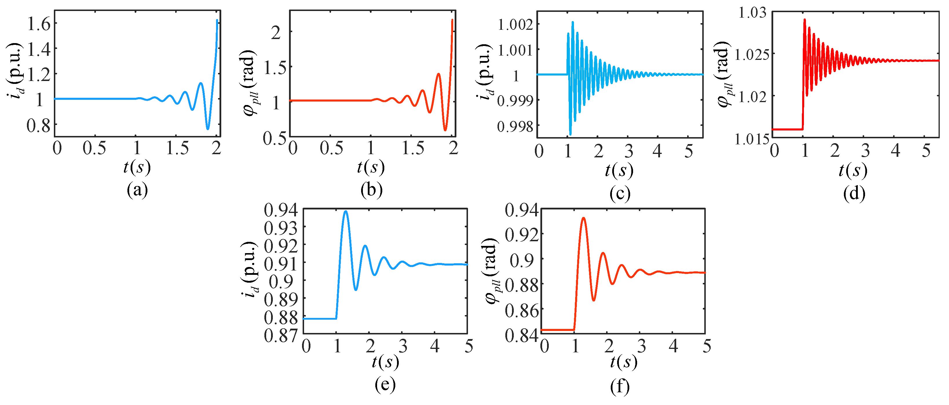
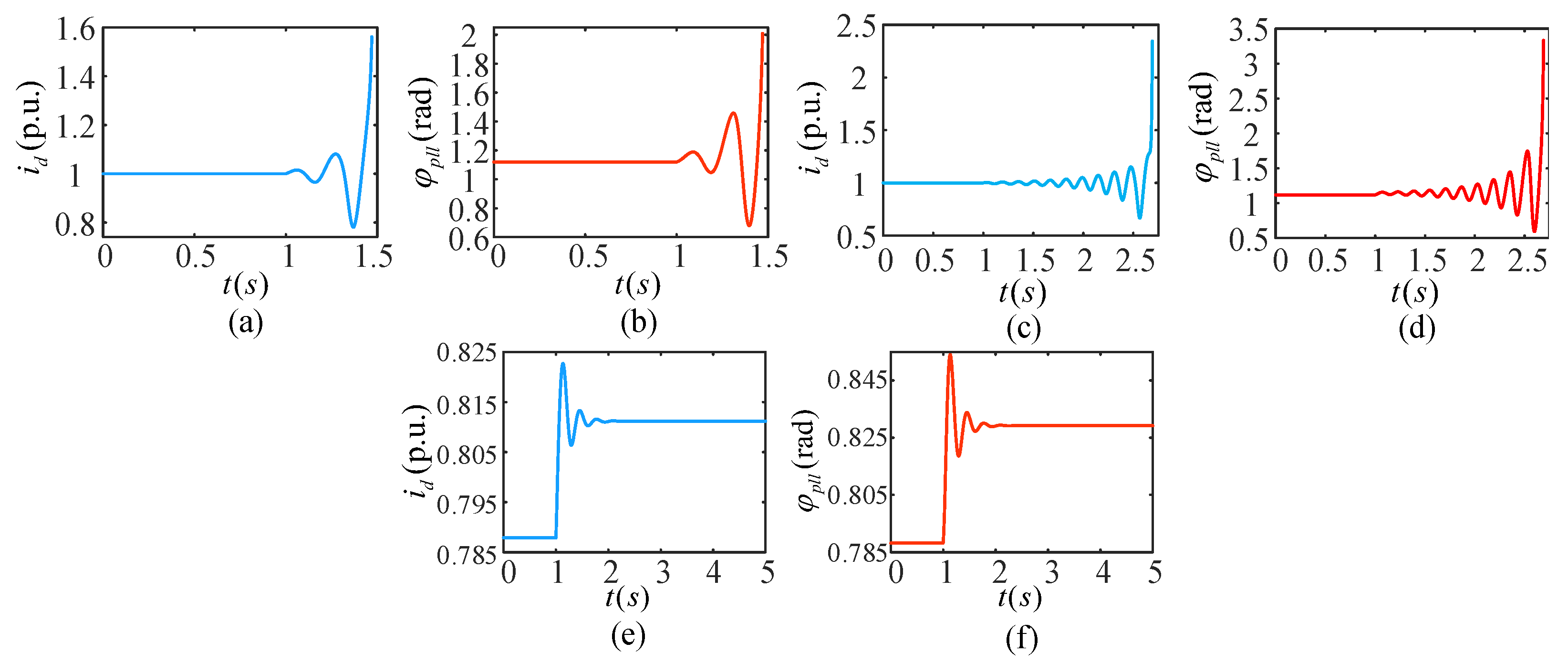
5.2. Verification of Time-Domain Simulation

Further, time-domain simulations are conducted in Matlab/Simulink (R2022a). For a comparative evaluation, $X_g$ is originally set to 0.85 p.u. and 0.9 p.u., respectively, in Figure 12 and Figure 13. The fault is set where $U_g$ drops from 1.0 p.u. to 0.98 p.u. at $t=1$ s. The time-domain waveforms of the state variables $i_d$ and ${\phi }_{pll}$ under this small disturbance in weak grids are illustrated in Figure 12 and Figure 13.

For Case A, a comparison of Figure 12a,b and Figure 13a,b clearly verifies that instability occurs at $X_g$ > 0.775 p.u. by an oscillatory divergence in both state variables. In contrast, for Case B, Figure 12c,d and Figure 13c,d also verify the above result of an oscillatory instability at $X_g$ > 0.878 p.u. well. In addition, for Case C in Figure 12e,f and Figure 13e,f, the system always remains stable and the original and final $i_{d0,s}$ values are apparently different from $i_{d0}$ = 1.0 p.u. All these perfectly verify the above analytical results.

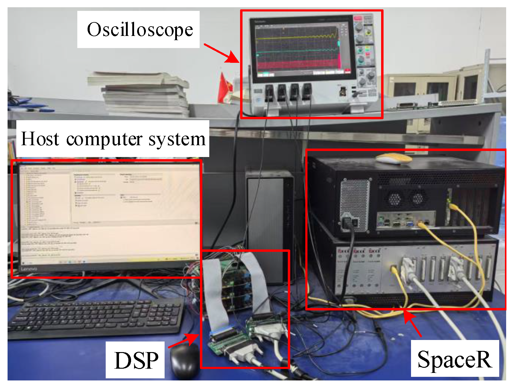
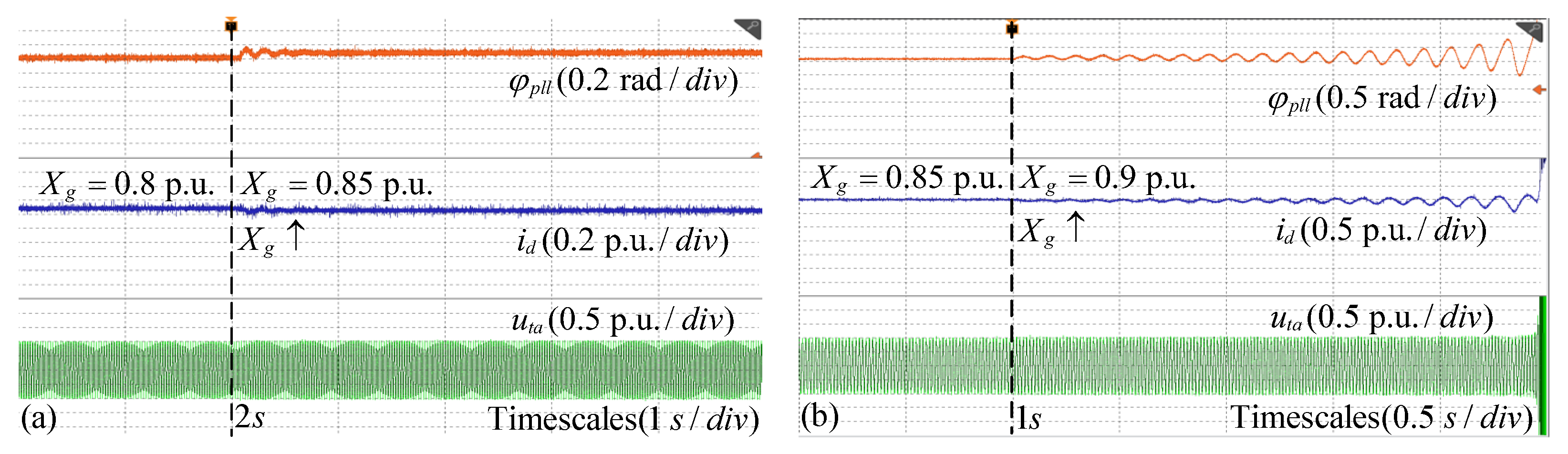
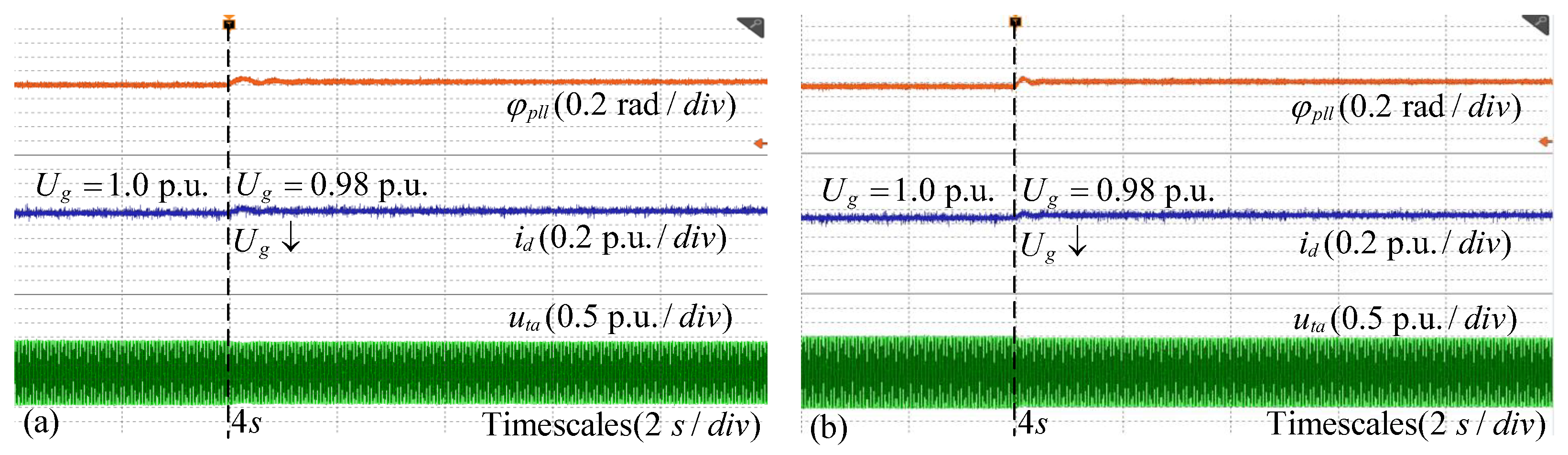
6. Experimental Verification

To validate the accuracy of the aforementioned results, hardware-in-the-loop experiments are conducted on the SpaceR platform. Figure 14 illustrates the experimental setup, which consists of a host computer system, SpaceR, digital signal processor (DSP), and oscilloscope. The host computer system serves as the operational interface, enabling iterative modifications to the experimental model and facilitating its transfer into the SpaceR module. The SpaceR provides a simulation environment that mimics real-world conditions for grid dynamics and transmits measurement signals to the DSP. The DSP simulates the dynamic behavior of GFL-VSC while providing feedback in PWM signals to SpaceR. The system parameters used in the experiments are identical to those employed in the time-domain simulation in Table A1. The experiments mainly investigate the small-signal stability of the GFL-VSC system under different response speeds of TVC for all three cases: A, B, and C.

For Case A, the line reactance $X_g$ is originally fixed at 0.75 p.u. A small disturbance is applied at t = 1 s by increasing $X_g$ to 0.05 p.u., i.e., $X_g$ becomes 0.80 p.u. The experimental waveforms of the phase angle ${\phi }_{pll}$, active current $i_d$, and phase-A terminal voltage $u_{ta}$ are presented in Figure 15. Clearly under this condition, the system exhibits oscillatory instability under a weak grid.

For Case B, two sets of experiments are conducted with $X_g$ fixed at 0.80 p.u. and 0.85 p.u., separately. As shown in Figure 16a,b, the system is initially stable, and a disturbance is applied to increase $X_g$ by 0.05 pu., i.e., $X_g$ becomes 0.85 p.u. and 0.90 p.u., respectively. The experimental waveforms of ${\phi }_{pll}$, $i_d$, and $u_{ta}$ are shown. In Figure 16a, the system can recover stability after being disturbed. In contrast, in Figure 16b, oscillatory instability occurs.

For Case C, the initial values of $X_g$ are set as $X_g$ = 0.85 p.u. and $X_g$ = 0.9 p.u., separately. As shown in Figure 4, if a disturbance is applied to increase $X_g$ by 0.05 p.u., the active current will show a significant change. This point is also clear in Figure 12e,f and Figure 13e,f. Therefore, in the test, a 0.02 p.u. voltage dip disturbance on $U_g$ is applied at t = 4 s. The results of ${\phi }_{pll}$, $i_d$, and $u_{ta}$ are depicted in Figure 17a,b, indicating well that the system can always recover stability after a small-signal disturbance.

Overall, the experimental results agree with the above analyses. Finally,

Table 1. Summary of response processes of TVC and their impacts on the GFL-VSC system under different response speeds.

	Case A: Considering TVC Dynamics	Case B: Considering TVC Rapid Response	Case C: Considering TVC Slow Response
Model difference	$U_t$ is controlled to track $U_{tref}$ while outputting $i_q$	$U_t$ = $U_{tref}$	$i_q$ = $i_{q0}$
Equilibrium point of active current	$i_{d0}$ = 1		$i_{d0,s}$ = 1 when $X_g$ < $X_{g,cr}$; $i_{d0,s}$ changes when $X_g$ > $X_{g,cr}$
Bifurcation form with respect to $X_g$	Sub-critical Hopf bifurcation		Trans-critical bifurcation
Synchronization and damping coefficients	$D_{total}$ becomes negative under weak gird		Always positive
Small-signal stability with respect to $X_g$	Unstable in weak girds		Always stable

summarizes the major results drawn from all different cases of TVC response speeds in the paper.

7. Conclusions

In summary, this paper has systematically investigated the effects of TVC on the GFL-VSC system by analyzing equilibrium points and small-signal stability under three scenarios: considering TVC dynamics, considering TVC rapid responses, and considering TVC slow responses. As the interaction analysis between different control loops within VSC is one of key problems in VSC grid-tied system stability, all these findings are significant for our deeper understanding of the role of TVC and are capable of providing valuable insights for stability and oscillation analyses. The main significant findings are as follows:

(1)

Different response speeds of TVC lead to distinct dynamic behaviors via different treatments of terminal voltage and reactive current in the modeling of the GFL-VSC system.

(2)

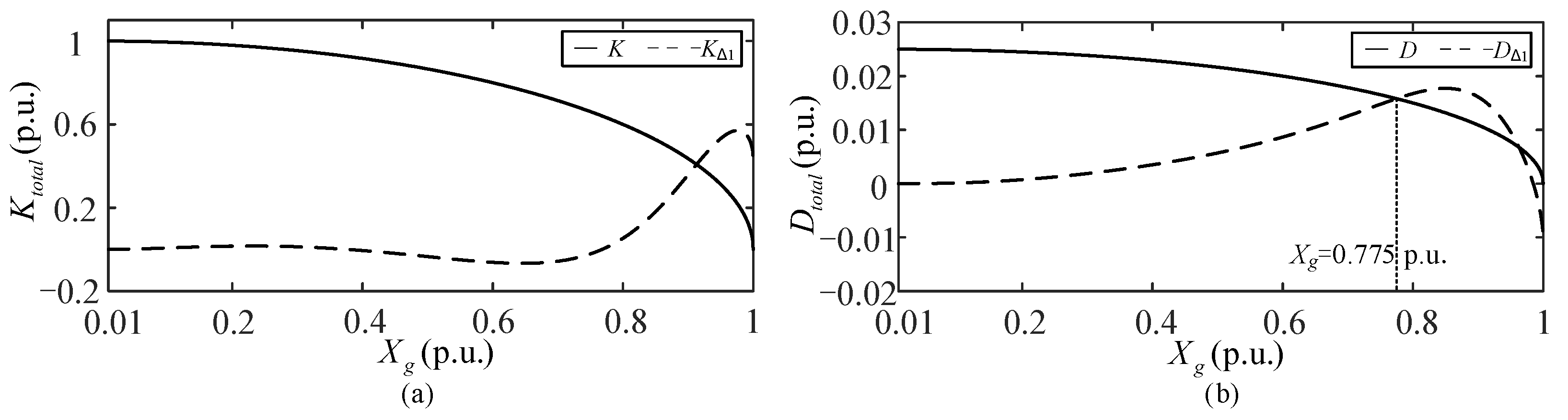
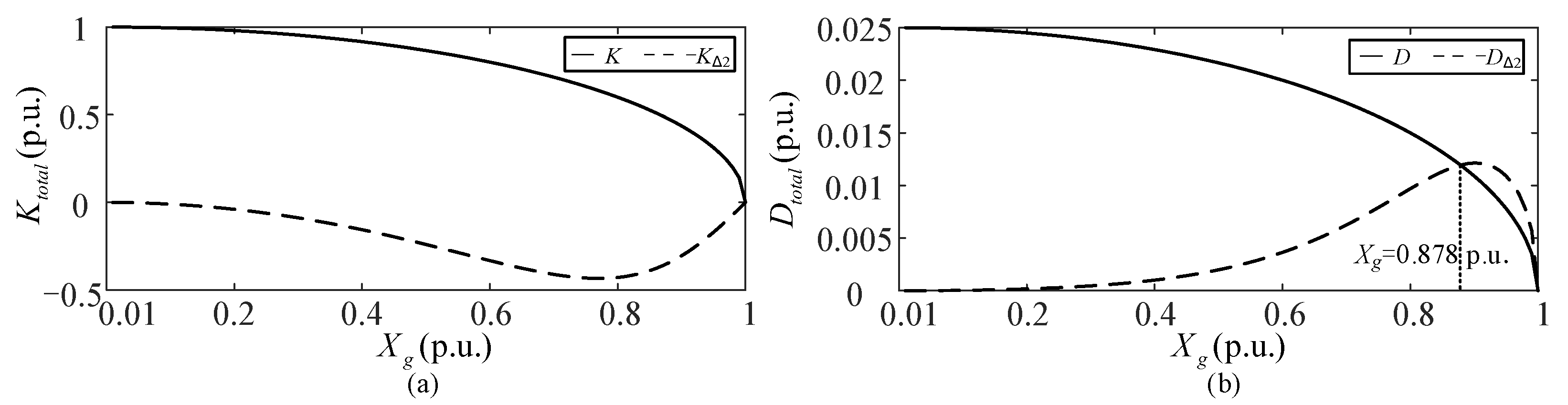
A comparative study between the scenarios of considering TVC dynamics and TVC rapid responses reveals that their impacts on the system are similar. This is because TVC participates in the dynamical process, constraining the equilibrium point of the active current $i_{d0}$ fixed as a constant value, which is independent of line reactance $X_g$. As $X_g$ increases, TVC dynamics introduce additional negative damping, causing $i_{d0}$ to undergo sub-critical Hopf bifurcation and leading to oscillatory instability in weak grids. Moreover, comparing their critical line reactances, when considering the TVC rapid response, the system exhibits a slightly larger stable region under weak grids.

(3)

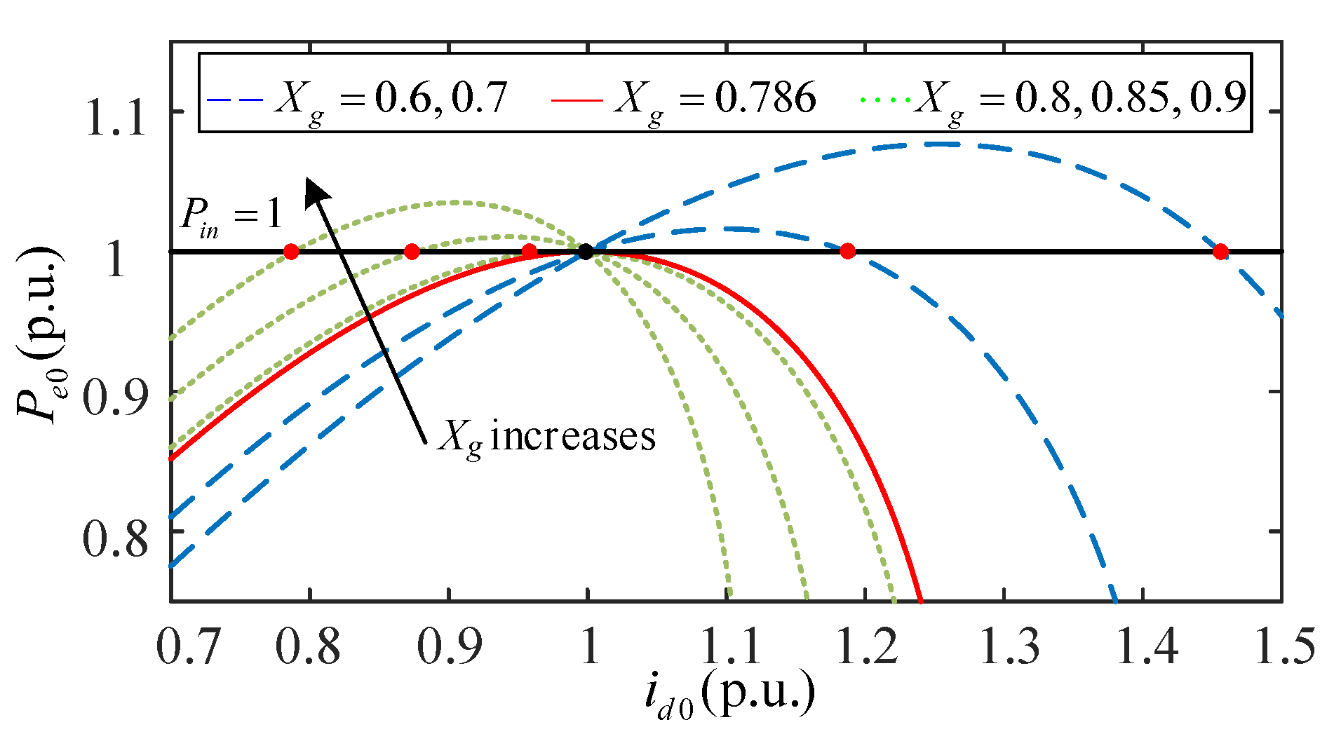
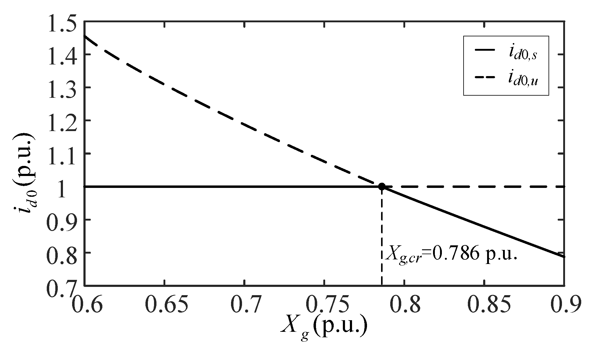
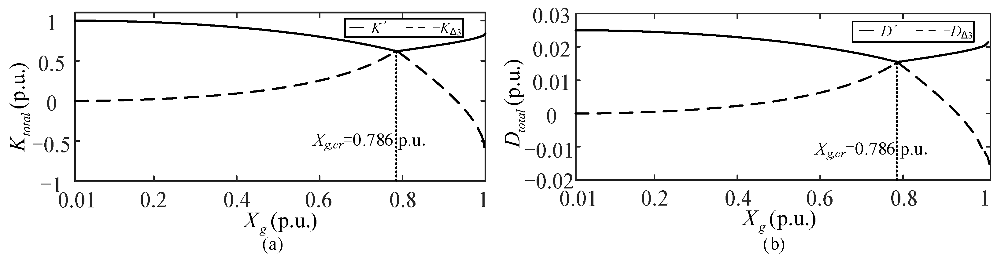
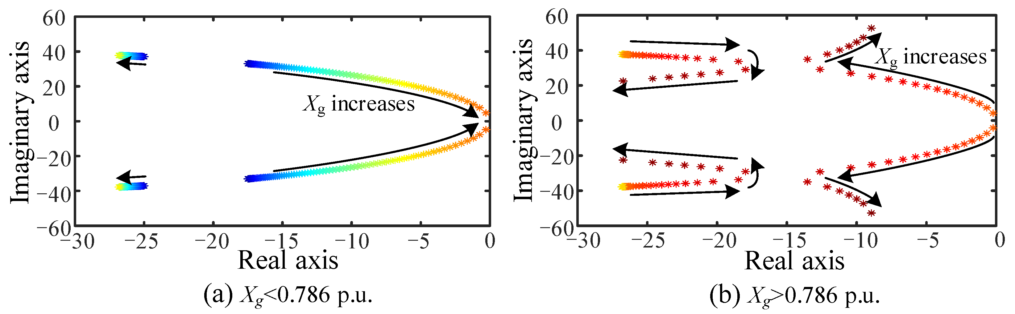
In contrast, for the scenario of considering TVC slow responses, the dynamics are completely different. By solving the relationships between the steady-state value of the active power $P_{e0}$ and $i_{d0}$, as well as $i_{d0}$ and $X_g$, the stable EP $i_{d0,s}$ and the unstable EP $i_{d0,u}$ are obtained. It is found that when $X_g<X_{g,cr}$, $i_{d0,s}=$ 1.0 p.u., identical to that in the previous two scenarios. However, when $X_g>X_{g,cr}$, the system undergoes trans-critical bifurcation, and the other EP $i_{d0,s}\ne$ 1.0 p.u. becomes stable. This stability transformation of the two EPs eliminates the negative damping effect and ensures the system is always small-signal stable. These novel phenomena have been completely ignored in all previous studies in the literature.

References

1. Operation of Renewable Energy Connected to the Grid in 2024; National Energy Administration of the People’s Republic of China: Beijing, China, 2025.
2. Zhu, B.; Liu, J.; Wang, S.; Li, Z. Enhanced Models for Wind, Solar Power Generation, and Battery Energy Storage Systems Considering Power Electronic Converter Precise Efficiency Behavior. Energies 2025, 18, 1320. [Google Scholar] [CrossRef]
3. Ji, X.; Liu, D.; Jiang, K.; Zhang, Z.; Yang, Y. Small-Signal Stability of Hybrid Inverters with Grid-Following and Grid-Forming Controls. Energies 2024, 17, 1644. [Google Scholar] [CrossRef]
4. Fu, X.; Huang, M.; Tse, C.K.; Yang, J.; Ling, Y.; Zha, X. Synchronization Stability of Grid-Following VSC Considering Interactions of Inner Current Loop and Parallel-Connected Converters. IEEE Trans. Smart Grid 2023, 14, 4230–4241. [Google Scholar] [CrossRef]
5. Zhou, Y.; Xin, H.; Wu, D.; Liu, F.; Li, Z.; Wang, G.; Yuan, H.; Ju, P. Small-Signal Stability Assessment of Heterogeneous Grid-Following Converter Power Systems Based on Grid Strength Analysis. IEEE Trans. Power Syst. 2023, 38, 2566–2579. [Google Scholar] [CrossRef]
6. Hu, B.; Zhao, C.; Sahoo, S.; Wu, C.; Chen, L.; Nian, H.; Blaabjerg, F. Synchronization Stability Enhancement of Grid-Following Converter Under Inductive Power Grid. IEEE Trans. Energy Convers. 2023, 38, 1485–1488. [Google Scholar] [CrossRef]
7. Zhang, Y.; Pen, H.; Zhang, X. Stability Control of Grid-Connected Converter Considering Phase-Locked Loop Frequency Coupling Effect. Energies 2024, 17, 3438. [Google Scholar] [CrossRef]
8. Liu, Y.; Zhu, L.; Xu, X.; Li, D.; Liang, Z.; Ye, N. Transient Synchronization Stability in Grid-Following Converters: Mechanistic Insights and Technological Prospects—A Review. Energies 2025, 18, 1975. [Google Scholar] [CrossRef]
9. Wang, X.; Taul, M.G.; Wu, H.; Liao, Y.; Blaabjerg, F.; Harnefors, L. Grid-Synchronization Stability of Converter-Based Resources—An Overview. IEEE Open J. Ind. Appl. 2020, 1, 115–134. [Google Scholar] [CrossRef]
10. Xie, Q.; Xiao, X.; Zheng, Z.; Wang, Y.; Song, D.; Du, K.; Zou, Y.; Zhang, J. An improved reactive power control strategy for LCC-HVDC to mitigate sending end transient voltage disturbance caused by commutation failures. Int. J. Electr. Power Energy Syst. 2023, 146, 108706. [Google Scholar] [CrossRef]
11. Wang, X.; Wu, H.; Wang, X.; Dall, L.; Kwon, J.B. Transient Stability Analysis of Grid-Following VSCs Considering Voltage-Dependent Current Injection During Fault Ride-Through. IEEE Trans. Energy Convers. 2022, 37, 2749–2760. [Google Scholar] [CrossRef]
12. Zhang, Y.; Han, M.; Zhan, M. The Concept and Understanding of Synchronous Stability in Power Electronic-Based Power Systems. Energies 2023, 16, 2923. [Google Scholar] [CrossRef]
13. Yuan, H.; Xin, H.; Huang, L.; Wang, Z.; Wu, D. Stability Analysis and Enhancement of Type-4 Wind Turbines Connected to Very Weak Grids Under Severe Voltage Sags. IEEE Trans. Energy Convers. 2019, 34, 838–848. [Google Scholar] [CrossRef]
14. Pei, J.; Yao, J.; Liu, R.; Zeng, D.; Sun, P.; Zhang, H.; Liu, Y. Characteristic Analysis and Risk Assessment for Voltage-Frequency Coupled Transient Instability of Large-Scale Grid-Connected Renewable Energy Plants During LVRT. IEEE Trans. Ind. Electron. 2020, 67, 5515–5530. [Google Scholar] [CrossRef]
15. He, X.; Geng, H. PLL Synchronization Stability of Grid-Connected Multi-Converter Systems. IEEE Trans. Ind. Appl. 2021, 58, 830–842. [Google Scholar] [CrossRef]
16. Kang, Y.; Lin, X.; Zheng, Y.; Quan, X.; Hu, J.; Yuan, X. The Static Stable-limit and Static Stable-working Zone for Single-machine Infinite-bus System of Renewable-energy Grid-connected Converter. Proc. CSEE 2020, 40, 4506–4515. (In Chinese) [Google Scholar] [CrossRef]
17. Zhang, Y.; Li, Y.; Gu, Y.; Green, T. Consideration of Control-Loop Interaction in Transient Stability of Grid-Following Inverters using Bandwidth Separation Method. In Proceedings of the 2023 11th International Conference on Power Electronics and ECCE Asia (ICPE 2023—ECCE Asia), Jeju Island, Republic of Korea, 22–25 May 2023; pp. 1294–1301. [Google Scholar] [CrossRef]
18. Wan, Y.; Wang, J.; Nan, D.; Zhang, B.; Xiong, X. Power Transfer Capacity Evaluation of Renewable Energy Delivery System Based on Grid-connected Inverter. Power Syst. Technol. 2024, 48, 171–183. (In Chinese) [Google Scholar] [CrossRef]
19. Yang, Z.; Ma, R.; Cheng, S.; Zhan, M. Nonlinear Modeling and Analysis of Grid-Connected Voltage-Source Converters Under Voltage Dips. IEEE J. Emerg. Sel. Top. Power Electron. 2020, 8, 3281–3292. [Google Scholar] [CrossRef]
20. Xiong, L.; Zhuo, F.; Wang, F.; Liu, X.; Chen, Y.; Zhu, M. Static Synchronous Generator Model: A New Perspective to Investigate Dynamic Characteristics and Stability Issues of Grid-Tied PWM Inverter. IEEE Trans. Power Electron. 2015, 31, 6264–6280. [Google Scholar] [CrossRef]
21. Hong, Z.; Cheng, M.; Zhan, M.; Yu, J.; Zhu, Y.; Wu, M. Interaction Analysis Between PLL-based Synchronization and Power Balance of Grid-Following Converters Tied to AC System. Proc. CSEE 2025, 1–16. (In Chinese) [Google Scholar]
22. Wang, D.; Liang, L.; Shi, L.; Hu, J.; Hou, Y. Analysis of Modal Resonance between PLL and DC-Link Voltage Control in Weak-Grid Tied VSCs. IEEE Trans. Power Syst. 2018, 34, 1127–1138. [Google Scholar] [CrossRef]
23. Ma, R.; Zhang, Y.; Zhan, M.; Cao, K.; Liu, D.; Jiang, K.; Cheng, S. Dominant Transient Equations of Grid-Following and Grid-Forming Converters by Controlling-Unstable-Equilibrium-Point-Based Participation Factor Analysis. IEEE Trans. Power Syst. 2023, 39, 4818–4834. [Google Scholar] [CrossRef]
24. Yuan, H.; Yuan, X.; Hu, J. Modeling of Grid-Connected VSCs for Power System Small-Signal Stability Analysis in DC-Link Voltage Control Timescale. IEEE Trans. Power Syst. 2017, 32, 3981–3991. [Google Scholar] [CrossRef]
25. Canay, I.M. A Novel Approach to the Torsional Interaction and Electrical Damping of the Synchronous Machine. Part I: Theory. IEEE Power Eng. Rev. 1982, PER-2, 24. [Google Scholar] [CrossRef]
26. Canay, I.M. A Novel Approach to the Torsional Interaction and Electrical Damping of the Synchronous Machine Part II: Application to an arbitrary network. IEEE Trans. Power Appar. Syst. 1982, PAS-101, 3639–3647. [Google Scholar] [CrossRef]
Figure 1. The figure shows the topology and control diagram of the GFL-VSC system.
Energies 18 03023 g001
Figure 2. The figure shows the d q and x y reference frames.
Energies 18 03023 g002
Figure 3. Plots of P e 0 variables and their intersection points with P i n as X g increases, when the model considering TVC slow responses is studied.
Energies 18 03023 g003
Figure 4. Plots of i d 0 versus X g when the model considering TVC slow responses is studied.
Energies 18 03023 g004
Figure 5. General equivalent Heffron–Phillips model of GFL-VSC system for all three cases, A, B, and C.
Energies 18 03023 g005
Figure 6. Plots of (a) synchronization coefficients (K and − K Δ 1 ) and (b) damping coefficients (D and − D Δ 1 ) with respect to X g for Case A: considering TVC dynamics.
Energies 18 03023 g006
Figure 7. Plots of (a) synchronization coefficients (K and − K Δ 2 ) and (b) damping coefficients (D and − D Δ 2 ) with respect to X g for Case B: considering TVC rapid responses.
Energies 18 03023 g007
Figure 8. Plots of (a) synchronization coefficients ( K and − K Δ 3 ) and (b) damping coefficients ( D and − D Δ 3 ) with respect to X g for Case C: considering TVC slow responses.
Energies 18 03023 g008
Figure 9. Case A (considering TVC dynamics) for (a) root locus plot as X g increases and (b) i d 0 with respect to X g to show sub-critical Hopf bifurcation. The solid line represents stable i d 0 , the dashed line represents unstable i d 0 , and dotted curves represent the unstable limit cycle.
Energies 18 03023 g009
Figure 10. Case B (considering TVC rapid responses) for (a) root locus plot as X g increases and (b) i d 0 with respect to X g to show sub-critical Hopf bifurcation. The solid line represents stable i d 0 , the dashed line represents unstable i d 0 , and dotted curves represent the unstable limit cycle.
Energies 18 03023 g010
Figure 11. Similar to Figure 9, but for Case C (considering TVC slow responses), including (a) under X g < X g , c r , and (b) under X g > X g , c r .
Energies 18 03023 g011
Figure 12. Time-domain waveforms of i d and φ p l l after a small disturbance in (a,b) for Case A, (c,d) for Case B, and (e,f) for Case C, under an originally weak grid, X g = 0.85 p.u.
Energies 18 03023 g012
Figure 13. Time-domain waveforms of i d and φ p l l after a small disturbance in (a,b) for Case A, (c,d) for Case B, and (e,f) for Case C, under an originally weak grid, X g = 0.9 p.u.
Energies 18 03023 g013
Figure 14. Photo of SpaceR real-time simulation platform.
Energies 18 03023 g014
Figure 15. Experimental results of Case A under a weak grid.
Energies 18 03023 g015
Figure 16. Experimental results of Case B under (a) X g = 0.8 p.u. and (b) X g = 0.85 p.u. in the initial state.
Energies 18 03023 g016
Figure 17. Experimental results of Case C disturbed by a 0.02 p.u. voltage dip on U g under (a) X g = 0.85 p.u. and (b) X g = 0.9 p.u.
Energies 18 03023 g017