Machine Learning and Multilayer Perceptron-Based Customized Predictive Models for Individual Processes in Food Factories

Abstract

A factory energy management system, based on information and communication technology, facilitates efficient energy management using the real-time monitoring, analyzing, and controlling of the energy consumption of a factory. However, traditional food processing plants use basic control systems that cannot analyze energy consumption for each phase of processing. This makes it difficult to identify usage patterns for individual operations. This study identifies steam energy consumption patterns across four stages of food processing. Additionally, it proposes a customized predictive model employing four machine learning algorithms—linear regression, decision tree, random forest, and k-nearest neighbor—as well as two deep learning algorithms: long short-term memory and multi-layer perceptron. The enhanced multi-layer perceptron model achieved a high performance, with a coefficient of determination (R²) of 0.9418, a coefficient of variation of root mean square error (CVRMSE) of 9.49%, and a relative accuracy of 93.28%. The results of this study demonstrate that straightforward data and models can accurately predict steam energy consumption for individual processes. These findings suggest that a customized predictive model, tailored to the energy consumption characteristics of each process, can offer precise energy operation guidance for food manufacturers, thereby improving energy efficiency and reducing consumption.

1. Introduction

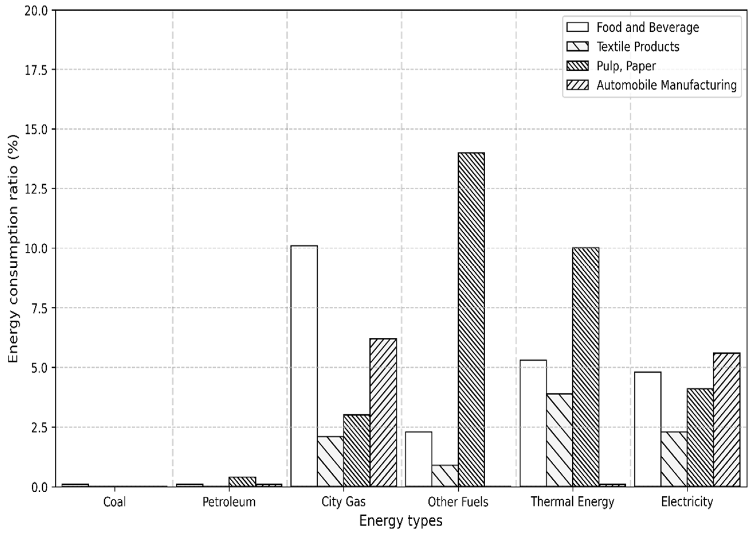
1.1. Current Status and Issues of Energy Consumption in the Industrial Sector

Energy consumption has become a significant global concern, leading to increased interest in reducing energy consumption and greenhouse gas emissions across various sectors. According to the 2022 domestic energy consumption statistics released by Korea’s Ministry of Trade, Industry, and Energy [1], the industrial sector consumes a total of 133,804,000 tons of oil equivalent (TOE). In addition, the food and beverage industry accounted for 2,558,000 TOE. Although the energy consumption of the food and beverage industry appears relatively small within the broader manufacturing sector, there is a growing demand for energy management systems that enhance energy efficiency, reduce costs, and minimize environmental impacts in this energy-intensive field. Consequently, initiatives to lower energy consumption and improve energy efficiency in the food industry are necessary. The analysis of energy usage in food factories indicates that their thermal energy consumption is substantial, comprising 59% for heating, 16% for cooling, 12% for mechanization, 8% for infrastructure, and 5% for other purposes. However, current energy management practices in food manufacturing plants are largely manual and lack the systems to systematically analyze or optimize energy consumption patterns for individual processes. Typically, equipment operators in food factories regulate energy by adjusting the temperature, pressure, and heating time based on empirical knowledge, making it difficult to maintain a consistent quality and achieve efficient energy operations.

In addition, energy is often supplied in excess of the required amount in conventional processes, and there is a lack of data-driven optimization systems to reduce this. Inefficient use of energy sources such as steam, electricity, and chilled heat leads to increased energy costs and greenhouse gas emissions. To address these challenges, an energy management system that undertakes real-time data collection and analyses, and then optimizes energy consumption data for each process, is crucial. The factory energy management system (FEMS) serves as a key technology to overcome these limitations. The implementation of FEMSs in manufacturing significantly enhances energy efficiency and reduces costs.

The 2022 energy usage across major manufacturing industries in South Korea is shown in Figure 1. In the food and beverage sector, energy consumption is primarily classified as city gas, thermal energy, electricity, and other fuels. The FEMS continuously monitors and controls a factory’s energy consumption, highlighting its role in promoting energy efficiency. For example, if the FEMS detects that a piece of equipment in the food factory is consuming excessive energy due to suboptimal operation during off-peak production hours, it can alert operators to adjust the system’s settings or reduce power inputs, thereby improving overall efficiency. The South Korean government has mandated the adoption of FEMSs for energy-intensive enterprises consuming over 10 million TOE, starting in 2025. For small and medium-sized enterprises consuming less than 10 million TOE, the government aims to expand the support for the dissemination of FEMSs in conjunction with smart factories, with a target of supporting more than 3000 new installations by 2040 [2].

1.2. Role and Importance of FEMS

The FEMS collects and analyzes energy consumption data in real time throughout food manufacturing processes. This enables control and optimization across the workflow, improving energy efficiency and reducing costs. As illustrated in Figure 2, prior studies primarily focused on energy management systems such as Building Energy Management Systems (BEMSs) and Energy Management Systems (EMSs), which targeted buildings or large plants [3,4]. Recently, the importance of FEMS within the manufacturing sector has intensified, as detailed energy monitoring and forecasting at the factory level have become achievable. Specifically, food manufacturing processes use various energy forms, including steam, electricity, and cooling [5,6]. The energy usage patterns vary considerably across different processes, necessitating the development of tailored control strategies [7,8]. Additionally, advancements in real-time data collection and analysis technologies now enable the precise tracking of energy consumption by processes, leading to an increase in applications that support process optimization based on these data [8,9,10]. Considering the direct relationship between energy usage and product quality in food factories, there is a need for comprehensive and customized prediction and management models that address energy conservation and the preservation of quality and production efficiency.

Recently, the cost of energy consumed in food production processes has been increasing, along with the rising cost of fossil fuels. Employing a FEMS can boost energy efficiency and lower overall energy consumption, thereby facilitating cost savings in food manufacturing facilities. In key food industry processes, such as heating and sterilization, a real-time performance assessment of sterilized products is difficult, leading to periodic evaluations. Consequently, manufacturers often provide more energy than the minimum requirement to ensure products’ quality. These challenges can be addressed by implementing a FEMS, installing measurement instruments for temperature, pressure, and flow and developing measurement and monitoring infrastructure like PLC/HMI systems. By comparing actual data with the theoretical energy supply in heating and sterilization processes, energy savings across the food industry can be achieved through precise measurement parameters and enhanced control valves.

1.3. Limitations of Existing Studies and the Necessity of This Study

This study aims to develop a customized predictive model to improve energy efficiency in food factories. Various studies recommend energy audits, real-time monitoring, and optimization models for reducing energy consumption in manufacturing sites [9,11,12,13]. Notably, researchers are forecasting energy usage in advance using data-driven modeling and machine learning techniques to manage peak consumption, in addition to reducing costs by adjusting production schedules or process conditions [14,15,16]. However, the food industry operates with various constraints such as product types, process-specific temperatures, humidity, and hygiene conditions, which result in a higher proportion of steam energy usage and more complex usage patterns compared to other manufacturing sectors [17,18].

In our previous study [19], we predicted electricity and Liquid Natural Gas (LNG) consumption for the entire process using multi-layer perceptron (MLP) and Support Vector Regression (SVR) algorithms. We evaluated the models’ performance with the coefficient of determination (R²) and a coefficient of variation of root mean square error (CVRMSE) as proposed by Geng et al. [20]. However, energy consumption predictions for individual processes within the target plant were not addressed. Furthermore, with the gradual implementation of an energy automatic control system in the food factory following the deployment of FEMSs, additional studies are necessary. This study introduces a tailored predictive model for four processes in a food factory based on FEMSs, refines the LNG predictive model from our previous study [19], and offers operational guidance.

1.4. Background and Motivation

Previously, MLP and SVR models were used to predict LNG energy consumption for an entire food factory [19], as shown in Figure 3a. The model’s performance was evaluated based on CVRMSE and R² following the guidelines in ASHRAE [20] and Webster and Bradford [21]. In addition, prediction accuracy was assessed by calculating the mean error rate of the predicted values in ASHRAE, and lastly the benchmark CVRMSE was set below 15% for monthly data and below 30% for hourly data. Our study utilized daily process data, establishing a CVRMSE under 20% and an R² above 0.75. However, after implementing a FEMS and establishing the baseline, energy consumption patterns shifted due to the transition from manual to automated control, as shown in Figure 4.

A previous study [19] predicted LNG consumption using MLP and SVR. Nevertheless, pattern changes after the application of a FEMS necessitated model retraining with recent data, as depicted in Figure 4. Furthermore, while a model was developed to forecast total LNG consumption for the food factory, no studies have addressed predicting steam energy consumption alongside LNG in individual processes. Therefore, changes in steam energy consumption patterns must also be considered, as shown in Figure 4b. After applying customized predictive models to each process, the predicted information should be provided to the energy information system (EIS) for a more detailed analysis of energy consumption patterns, as presented in Figure 3b.

In this study, the introduction of FEMSs to food factories is proposed, achieving energy-saving effects, and with the suggestion of a customized predictive model optimized for individual processes. This approach delivers high-accuracy guidance for operating individual processes and enhances operational efficiency by automatically suggesting optimal predictive models tailored to the characteristics of each process. This study aims to enhance energy efficiency in food factories.

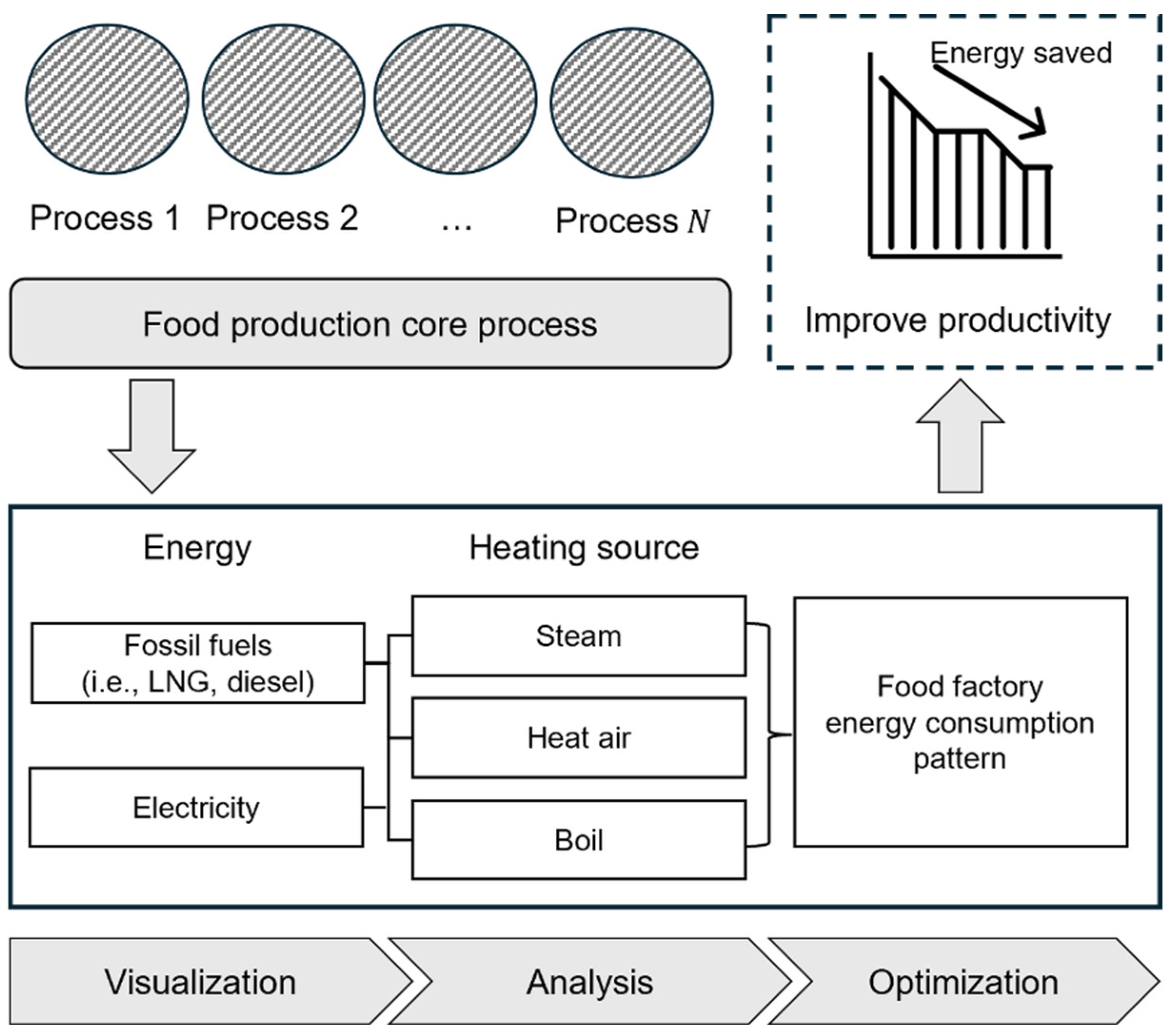
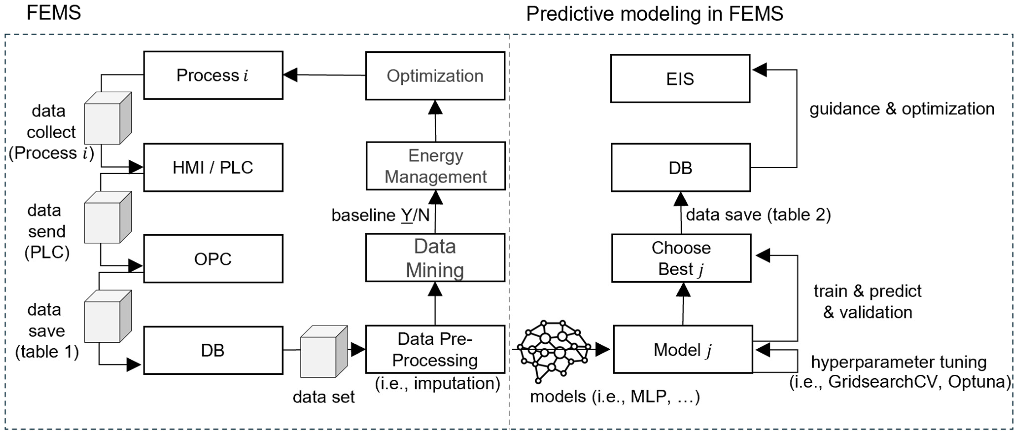
2. Customized Predictive Modeling Approach

As illustrated in Figure 5, in a food factory employing a FEMS, data are collected at predetermined intervals throughout the food production process using Human–Machine Interface (HMI) systems and Programmable Logic Controller (PLC) equipment. Specifically, the data gathered by the PLC are stored in a database via server–client communication using the Open Platform Communications (OPC) protocol. These stored data are then preprocessed and utilized to identify energy consumption patterns and monitor energy usage, thereby establishing a baseline for the food production process. Once this baseline is established, energy consumption shifts from manual to automatic control, enabling the optimization of energy use based on the baseline. Additionally, the conventional FEMS in the food factory employs predictive models to forecast total LNG and electricity consumption. However, since each process has distinct characteristics, their energy consumption patterns vary, necessitating more detailed predictive modeling. Therefore, this study proposes a customized predictive model for each individual process within the food production system.

The methodology includes preprocessing data for each specific process using four machine learning algorithms, including LSTM and MLP models, followed by training the models with the processed data. The model j with the highest predictive performance is selected as the optimal model for the i-th food production process, and the predicted values and performance metrics of all trained models are saved. A model achieving such a predictive accuracy is considered highly reliable. If the reliability of all the models remains low, their reliability is enhanced by retraining them using the entire dataset 1000 times. Highly reliable models offer operational guidance to operators, thereby optimizing process operations, improving energy efficiency, and potentially reducing absolute energy consumption. This chapter initially details the data collection and preprocessing techniques for the customized predictive modeling of each individual process, subsequently addressing the evaluation and validation of each predictive model.

2.1. Data Collection and Preprocessing

Effective data collection and preprocessing are vital for forecasting energy-efficient consumption in food manufacturing. In this study, data were sourced from an operational food factory implementing a FEMS, upon which a customized predictive model for individual processes was developed. In the subsequent sections, the data collection and preprocessing processes are described, with a correlation analysis.

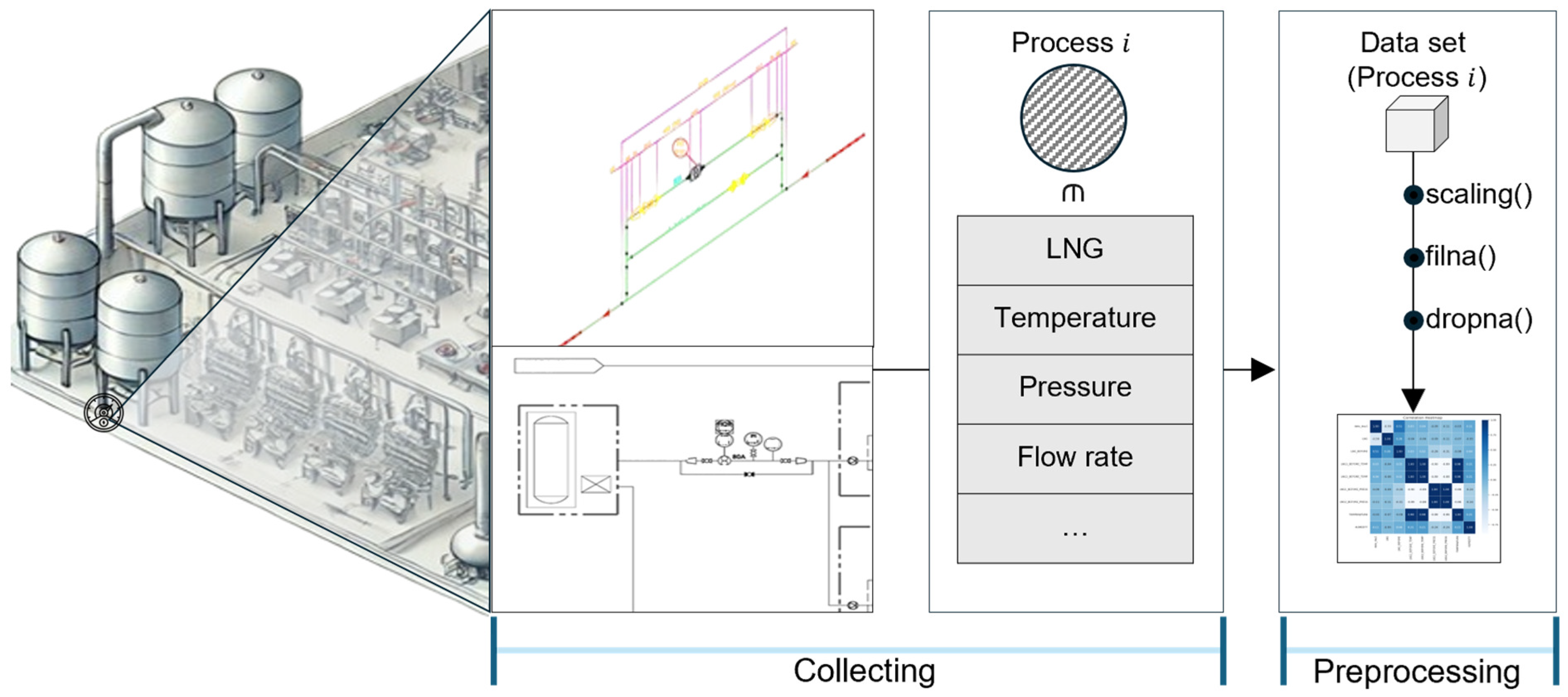
2.1.1. Data Collection

As illustrated in Figure 6, sensors were deployed across processes to capture data at one-second intervals. The dataset includes key variables influencing each process’s energy consumption patterns, such as temperature, pressure, flow rate, and external environmental factors. Real-time data acquisition was facilitated through HMI and PLC systems, and data were stored in a database using the OPC protocol from December 2021. To target daily energy consumption predictions, the high-frequency data were aggregated into daily totals, reducing excessive granularity and reflecting actual plant operational patterns. Data collection within the food factory environment encountered several challenges. For example, it was conducted in alignment with equipment maintenance schedules to avoid disrupting production, and additional infrastructure was established to support the application of the FEMS. Additionally, to minimize data loss due to instrument malfunctions in certain processes, extra sensors were installed, or data from those sections were synchronized with HMI data.

2.1.2. Data Preprocessing

The collected data were then preprocessed to ensure appropriate formatting for the prediction model. Effective preprocessing enhances the model’s performance, which runs through the following steps:

• Data normalization is a crucial step in preprocessing to eliminate bias arising from scale disparities between variables during model training. In this study, min-max scaling was employed to rescale all variable values to a uniform range of 0 to 1. This transformation is achieved using the following equation:

$$X_{minmax}={\displaystyle \frac{X-X_{min}}{X_{max}-X_{min}}}$$

(1)

 

Min–max scaling facilitates faster convergence in the MLP model and is particularly advantageous when the data do not follow a normal distribution;

• Handling missing values: The dataset consisted of 624 data points, with periods of no measurements—such as factory shutdowns or network failures (e.g., 23 March 2022–4 May 2022; 15 May 2023–2 January 2024; 6 March 2024–30 May 2024)—excluded entirely. Within these 624 data points, approximately 21.5% contained missing values, primarily due to non-operational days such as weekends and holidays. These non-consecutive missing values were addressed through linear interpolation using Pandas’ interpolate and fillna functions to maintain data continuity, which is crucial for time-series energy consumption data. Linear interpolation was chosen for its simplicity and effectiveness, as the missing values on non-operational days reflect predictably low or zero energy use, minimizing any impact on the model’s accuracy. Although energy data can exhibit non-linear patterns, the limited scope of these non-consecutive gaps ensured that linear interpolation did not significantly distort the dataset;
• Handling outliers: Outliers, such as negative values or NaN, arise from abnormal process operations and data entry errors. Statistical methods identified outliers as values exceeding 3σ from the mean for each variable. These outliers were subsequently managed with linear interpolation.

During data preprocessing, missing values and outliers were handled according to our criteria. However, considering that the total number of days from the start of data collection to 1 January 2025, is 1122 days, and 761 days excluding holidays and weekends, the proportion of the processed data is 15.78%. We detected changes in control modes using k-means clustering (k = 3) and incorporated this as a new feature to enhance the adaptability of the model.

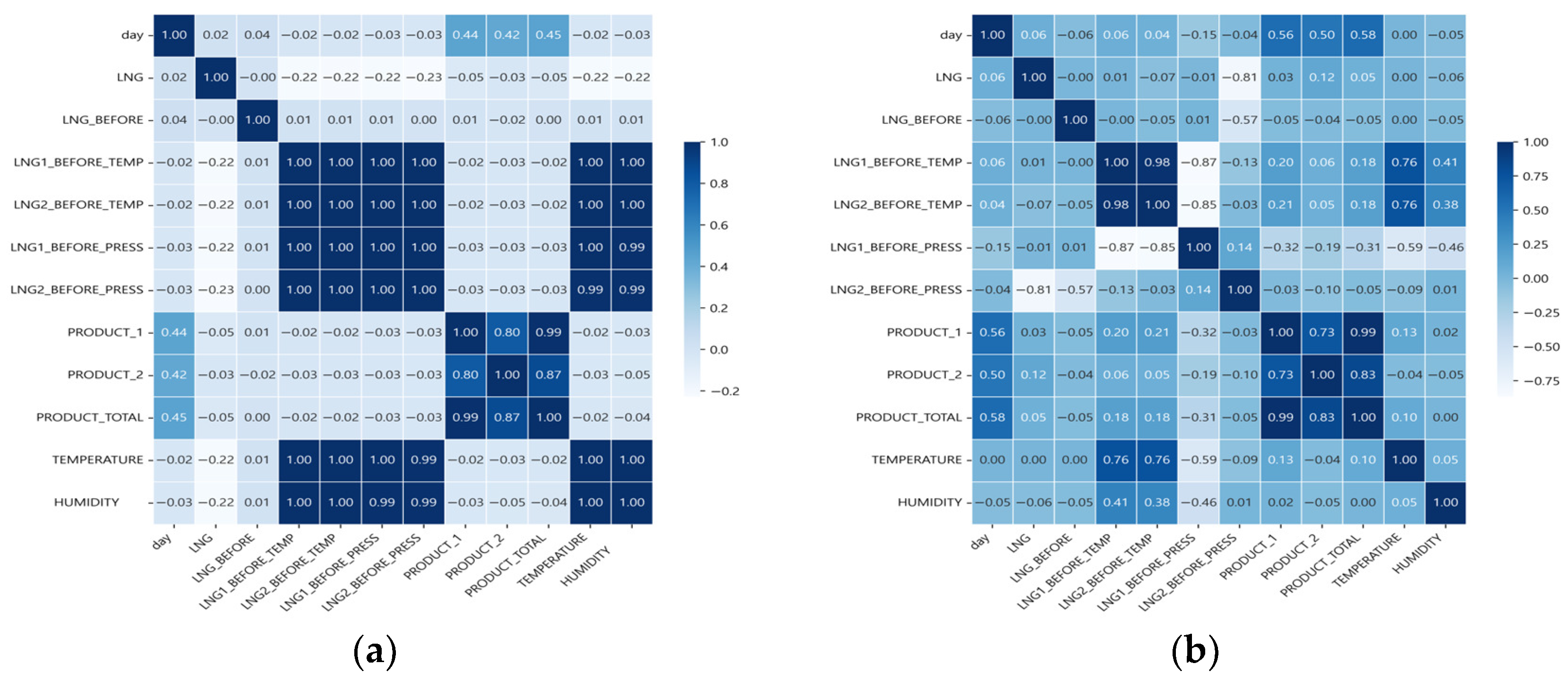
2.1.3. Correlation Analysis

To ensure consistency and reliability in our prediction model, we selected the input variables based on our previous study [19]. The Pearson correlation coefficients between these variables were calculated to assess their linear relationships and visualized using Seaborn heatmaps: Figure 7 presents the correlation data for a 3-month period, while Figure 8 summarizes the correlations across the entire duration of the process. The key features analyzed are listed in

Table 1. Description of heatmap features.

Feature	Unit	Description
day	1~7	Day of the week (i.e., Monday: 1~Sunday: 7)
LNG	Nm3	LNG consumption of the day
LNG_BEFORE	Nm3	Previous day’s LNG consumption
LNG1_BEFORE_TEMP	°C	Previous day’s LNG temperature at food factory 1
LNG2_BEFORE_TEMP	°C	Previous day’s LNG temperature at food factory 2
LNG1_BEFORE_PRESS	kPa	Previous day’s LNG pressure at food factory 1
LNG2_BEFORE_PRESS	kPa	Previous day’s LNG pressure at food factory 1
PRODUCT_1	kg	Production volume of food factory 1
PRODUCT_2	kg	Production volume of food factory 2
PRODUCT_TOTAL	kg	Production volume of food factories 1 and 2
TEMPERATURE	°C	Average outdoor temperature of the previous day
HUMIDITY	%	Average outdoor humidity of the previous day

.

• In Figure 7, LNG exhibits a strong positive correlation with PRODUCT_TOTAL (0.92) and PRODUCT_1 (0.91), suggesting that increased LNG consumption is associated with higher production levels. This strong correlation suggests that production is a key predictor, improving the model’s explanatory;
• Furthermore, LNG1_BEFORE_TEMP and LNG1_BEFORE_PRESS (−0.90), as well as LNG2_BEFORE_TEMP and LNG2_BEFORE_PRESS (−0.89), display strong negative correlations, highlighting the automatic control relationship between temperature and pressure;
• HUMIDITY has a weak correlation with most variables, is unrelated to production and LNG, and displays a weak correlation with day (LNG −0.59, LNG_BEFORE 0.51), indicating a temporal trend. LNG and TEMPERATURE exhibit a strong negative correlation, highlighting the influence of weather on energy input;
• Figure 8a shows correlation coefficients near zero, indicating weak relationships;
• Figure 8b shows that the correlation coefficients among LNG1_BEFORE_TEMP, LNG2_BEFORE_TEMP, TEMPERATURE, and HUMIDITY decreased from 1.00 to between 0.27 and 0.97, demonstrating reduced redundancy. Correlations increased between LNG and PRODUCT_1 (0.03), PRODUCT_2 (0.12), and PRODUCT_TOTAL (0.05). Additionally, the correlation between LNG and day remained stable at a weak positive value of 0.06, despite an apparent intent to suggest a slight increase. This shift likely results from changes in operational patterns due to seasonal variations and the implementation of automatic control.

In the full-period data, preprocessing enhanced the correlation between LNG and the key variables. Specifically, the correlation between LNG and day changed from −0.59 in the three-month data to 0.06 for the entire period, reflecting seasonal changes and operational adjustments. Preprocessing reduces variable redundancy and clarifies correlations, thereby providing valuable data for prediction models. However, due to alterations in consumption patterns from energy-saving measures, the LNG consumption prediction model requires improved and customized steam energy prediction models to be developed for each process.

2.2. Development of LNG Consumption Prediction Models

2.2.1. MLP-Based LNG Consumption Prediction

A prior study [19] introduced a predictive model using MLP and SVR algorithms, demonstrating enhanced performance over SVR alone, with a CVRMSE of 12.52% and an R² of 0.88. This study aims to enhance the MLP-based model using preprocessing methods from Section 2.1, in addition to recent process data.

• Dataset and preprocessing: For the small sample size scenario outlined in

  Table 2. Model implementation specifications.

  LNG consumption prediction dataset range	Small sample size case	January 2 to April 14 of 2024 (90 rows calibration dataset)
  		August 19 to November 24 of 2024 (91 rows calibration dataset)
  	Large sample size case	December 7 of 2021 to January 1 of 2025 (624 rows calibration dataset, 422 rows excluding weekends dataset)
  Individual processes prediction dataset	Small sample size case	August 17 to November 29 of 2024 (105 rows 1st process calibration dataset)
  		August 18 to November 29 of 2024 (69 rows 2nd process calibration dataset)
  		June 3 to November 29 of 2024 (166 rows 3rd process calibration dataset)
  		June 3 to November 29 of 2024 (167 rows 4th process calibration dataset)

  , data were gathered from 2 January 2024 to 14 April 2024 (90 rows) and from 19 August 2024 to 24 November 2024 (91 rows). In the large sample size scenario, data were collected from 7 December 2021 to 1 January 2025 (624 rows, excluding weekends and holidays). Missing values were addressed using linear interpolation and normalized through min–max scaling;
• Hyperparameter optimization: Optimization was executed using Optuna and GridSearchCV. Optimal parameters were identified by varying hidden layer sizes, learning rate, max iter, and solver (

  Table 3. Hyperparameters of MLP model.

  Hyperparameter	Hyperparameter Calibration (Small Sample Size)	Hyperparameter Calibration (Large Sample Size)
  Activation	ReLU	ReLU
  Alpha	1.0721	0.0004
  Batch size	Auto	auto
  Hidden layer size	112	57
  Learning rate	adaptive	adaptive
  Max iteration	482	421
  Solver	LBFGS	LBFGS
  Tol	0.0001	0.0073

  );
• Model training and performance: The MLP model, trained with optimized hyperparameters, was assessed for performance in scenarios involving both small and large sample sizes. When evaluated with a smaller dataset, the model exhibited a satisfactory accuracy and fit, as indicated by the performance metrics. However, with a larger dataset, the model showcased significantly better performance metrics, underscoring its improved accuracy and goodness of fit.

The model demonstrates significantly improved performance metrics with larger sample sizes, marking a substantial enhancement over the previous study [19]. This improvement was achieved by integrating recent process data, systematic data preprocessing, and optimized hyperparameters. Comprehensive performance metrics, including cross-validation results, are detailed in Section 2.4.

As illustrated in Figure 9, for substantial sample sizes, we selected the energy consumption prediction model requiring retraining and executed retraining by iterating the entire dataset for each process 1–1000 times. Notably, the performance metrics improved when the MLP model underwent multiple retrains; thus, we aimed to optimize the predictions of LNG energy consumption.

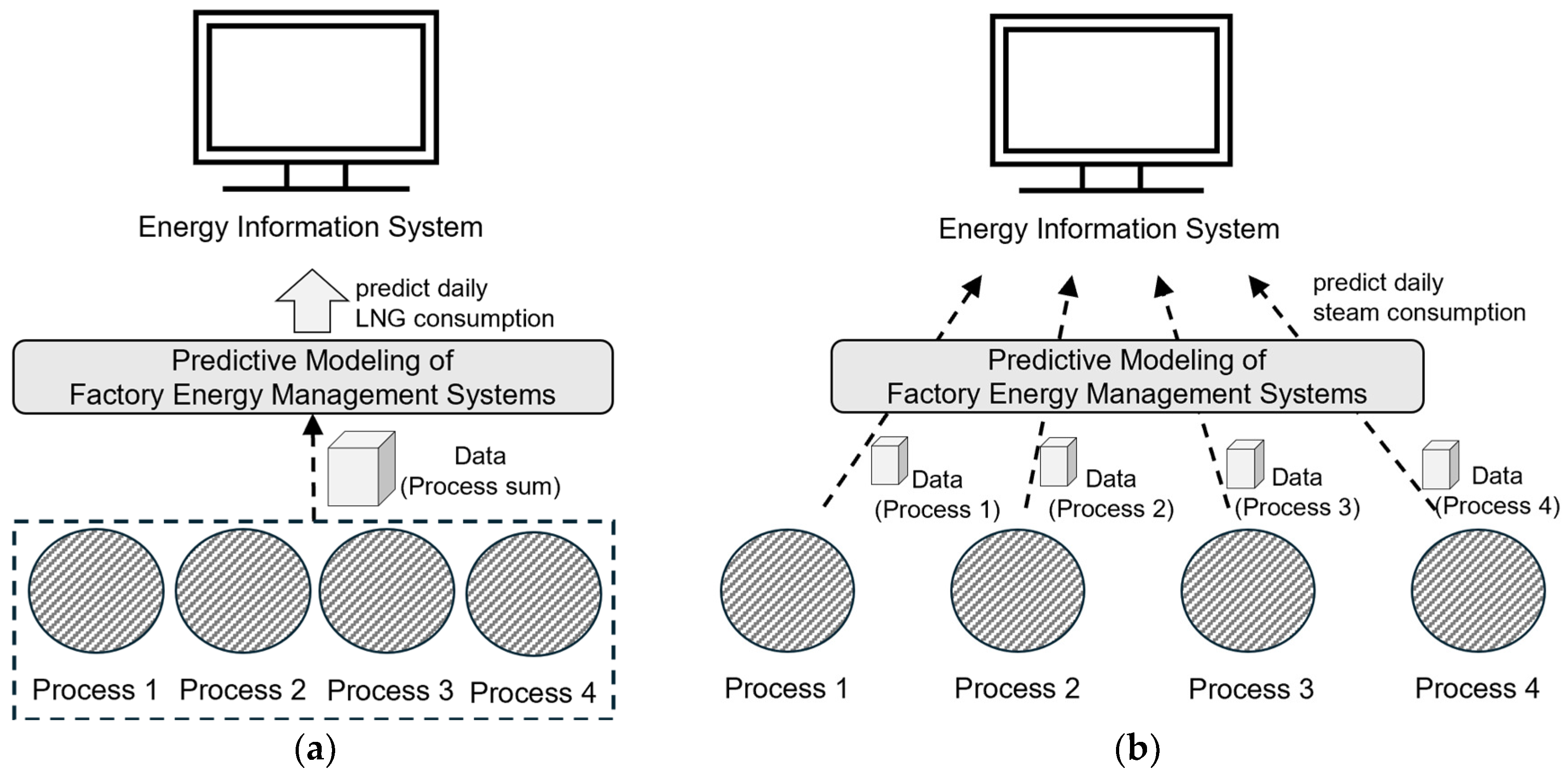
2.2.2. Customized Predictive Models

Beyond the prediction of LNG consumption, this study introduces a tailored predictive model for steam energy consumption across four distinct processes (1st, 2nd, 3rd, and 4th) within a food factory. As highlighted in Section 1, energy consumption patterns vary significantly across processes owing to their unique operational characteristics. (e.g., variations in control methods, temperature, pressure, and production schedules). Consequently, a single model applicable to all scenarios may not be sufficient for accurate steam energy predictions. The proposed approach involves training multiple machine learning models and MLP models for each process and selecting the best-performing model to provide customized guidelines.

• Dataset: The dataset for forecasting steam energy consumption across individual processes is detailed in Table 2. These datasets were gathered following the methodology outlined in Section 2.1.1, with data preprocessing steps—such as linear interpolation and min–max scaling for handling missing values—consistently applied to ensure data integrity;
• Model selection and training: For the four food production processes, we utilized linear regression (LR), decision tree (DT), random forest (RF), k-nearest neighbors (KNN), long short-term memory (LSTM), and MLP models. These six models were benchmarked against the baseline persistence model. To guarantee model robustness, k-fold cross-validation was employed during training, as described in Section 2.4.2;
• The performance of each model was evaluated using five metrics: CVRMSE, R², relative accuracy (100—mean error rate), MAE, and RMSE;
• Best model selection: The best model for each process was ranked using CVRMSE as described in Section 2.4.1.

Among the two performance metrics mentioned above, an R² near 1 and a lower CVRMSE indicated improved performance. Models exhibiting these metrics effectively capture steam energy consumption patterns in individual processes, providing reliable guidance for energy optimization.

2.3. Optimization of MLP Prediction Model

To achieve ab optimal prediction performance for LNG consumption in food factories and steam energy consumption in individual processes, hyperparameter optimization of the MLP model is essential. As detailed in Section 2.2, the MLP demonstrated excellent capability in capturing energy consumption patterns. However, it is crucial to finely tune the MLP model’s hyperparameters to align with specific characteristics. This study applied the hyperparameter optimization methods described in previous studies [22,23,24,25,26] and derived the optimal hyperparameters for the MLP prediction model of energy consumption in FEMS-based food factories.

Hyperparameter Optimization

In the literature, a variety of strategies are used to optimize MLP hyperparameters, from fully automated searches to entirely manual tuning. For example, Reference [22] utilizes an Optuna-based Bayesian optimization approach to fine-tune MLP parameters, reporting a substantial accuracy improvement over default settings. Similarly, Reference [23] adopts the HyperOpt library’s Tree-structured Parzen Estimator (TPE) for Bayesian hyperparameter exploration. These automated frameworks systematically sample and evaluate hyperparameter combinations, reducing trial and error and often outperforming manual tuning. In contrast, Reference [24] follows a manual, iterative protocol grounded in domain expertise and validation feedback. While straightforward, this manual strategy is time-consuming and offers no guarantee of a global optimum. Together, these studies illustrate the trade-off between the principled thoroughness of automated methods (e.g., Optuna, HyperOpt) and the intuitive, incremental adjustments characteristic of manual tuning [22,23,24].

Beyond search methodologies, prior work emphasizes the critical role of structural and training-related hyperparameters in MLP performance. Reference [25], for instance, highlights the importance of regularization and optimizer selection: applying dropout to randomly disable units during training mitigates overfitting, while comparing SGD and Adam optimizers shows that although Adam converges more rapidly, SGD can sometimes yield a better generalization—suggesting that Adam’s accelerated updates may slightly increase generalization errors, whereas SGD’s slower updates can improve the final performance. Meanwhile, Reference [26] underscores how learning-rate schedules enhance convergence stability and avoid poor local minima, and it demonstrates that L₂ weight decay further bolsters generalization. Collectively, these studies [25,26] show that choices of optimizer algorithm, learning-rate schedule, dropout rate, and weight decay profoundly shape MLP training dynamics and generalization.

Building on References [22,23,24,25,26], our study integrates advanced automated tuning with rigorous validation to optimize MLP hyperparameters. We employ Optuna’s Bayesian optimization to explore key settings—number of hidden layers, neurons per layer, learning rate, batch size, and dropout ratio—in a define-by-run framework that leverages pruning to streamline the search. Concurrently, we incorporate scikit-learn’s GridSearchCV to exhaustively evaluate the most promising subregions identified by Optuna. This hybrid strategy ensures both breadth and depth: Optuna narrows the search to high-potential areas, and GridSearchCV then meticulously fine-tunes combinations within those areas. A further distinguishing feature is our PyTorch 2.4.1-based rolling-window cross-validation tailored to time-series data. Unlike standard k-fold cross-validation, rolling-window validation respects temporal order by training on an initial sequential window and validating on the immediately subsequent period, then sliding the window forward to repeat the process. Inspired by Reference [23], we train on all data except the most recent 30 days and evaluate on that held-out period, using an 80%/20% train/validation split for large-sample cases to minimize overfitting. This time-aware approach more realistically assesses each configuration’s ability to generalize to future data, mitigating temporal bias. To expedite computation, we harness CUDA-enabled GPU parallelization, completing 500 trials within 20–40 min. The effectiveness of this hybrid optimization and validation is illustrated below:

• Figure 10a shows the Optuna convergence curve for small-sample data (e.g., LNG consumption prediction), where the MLP reaches an MSE of 0.0302 in 500 trials. Despite the low MSE (red dotted line), the coefficient of variation of the RMSE (CVRMSE = 7.29%) and R² = 0.96 confirm reliable generalization;
• Figure 10b presents the large-sample scenario: rolling-window validation prevents overfitting, yielding an MSE of 0.0556, CVRMSE = 18.38%, and R² = 0.87. CUDA-enabled GPU parallelization ensures these 500 trials are completed in just 20–40 min;
• Figure 10c–f validate tuning for individual steam-consumption processes, with MSEs ranging from 0.0343 to 0.0686. Additionally, although a low MSE could suggest overfitting, we concurrently assessed the CVRMSE and R² to ensure the model’s reliability. Detailed calibrated hyperparameters are provided in

  Table 4. Hyperparameters of the 2nd calibration MLP model.

  Hyperparameter	2nd Calibration (Small Sample Size)	2nd Calibration (Large Sample Size)	1st~4th Individual Processes
  Activation	tanh	ReLU	tanh
  Alpha	0.000001	0.02306047461918005	0.000001
  Batch size	auto	auto	auto
  Hidden layer size	(150, 150, 150)	(50, 50, 50)	(150, 150, 150)
  Learning rate	adaptive	adaptive	Adaptive
  Solver	LBFGS	Adam	LBFGS
  Tol	1.95 × 10−4	1.72 × 10−5	1.95 × 10−4
  Epochs	482	259	482

  .

2.4. Evaluation Methodology

2.4.1. Performance Metrics

In the previous section, an MLP model was implemented for the prediction of LNG consumption and an MLP model for the prediction of steam consumption across four distinct processes in food production, followed by optimization through hyperparameter tuning. This hyperparameter optimization enhanced the model’s performance, necessitating a performance metric analysis to evaluate the prediction model used in this study. The performance of the proposed energy consumption prediction model is calculated using the formula below, with the variables defined as follows: $y_i$ denotes the actual value, ${\widehat{y}}_i$ denotes the value predicted by the model, $\overline{y}$ indicates the mean of the actual values, and n represents the number of data points.

$$CVRMSE={\displaystyle \frac{\sqrt{\frac{1}{n}{\sum }_{i=1}^n{\left(y_i-{\widehat{y}}_i\right)}^2}}{\overline{y}}}\times 100$$

(2)

$$R^2=1-{\displaystyle \frac{{\sum }_{i=1}^n{\left(y_i-{\widehat{y}}_i\right)}^2}{{\sum }_{i=1}^n{\left(y_i-\overline{y}\right)}^2}}$$

(3)

$$MAE=\frac{1}{n}\sum _{i=1}^n\left|y_i-{\widehat{y}}_i\right|$$

(4)

$$RMSE=\sqrt{{\displaystyle \frac{1}{n}}\sum _{i=1}^n{\left(y_i-{\widehat{y}}_i\right)}^2}$$

(5)

$$RelativeAccuracy=100-\left({\displaystyle \frac{MAE}{\overline{y}}}\times 100\right)$$

(6)

Using these indicators, the model’s prediction accuracy and error, which are essential to assess the model’s reliability, were quantitatively assessed.

2.4.2. Cross-Validation Strategy

In the previous section, we conducted hyperparameter tuning on the MLP model to predict LNG and steam consumption, optimizing its performance and evaluating it with various metrics. Nevertheless, validating the model’s performance with a single train–test split remains challenging. Specifically, since the energy consumption data in this study exhibit time-series characteristics, a cross-validation strategy that accommodates time-series data, rather than traditional random cross-validation, is necessary. Therefore, we employed time series cross-validation to evaluate the predictive performance of the model. We used time series cross-validation to maintain the temporal order of the data. This method avoids the unrealistic scenario of predicting past data using future data and more accurately reflects the model’s performance in a real operational environment. The procedure is as follows:

• Data splitting: After sorting the entire dataset chronologically, the initial training set comprises past data, with the subsequent interval used for validation. For example, if the data comprise daily consumption from January to November 2024, the initial training set contains data from January–September, and the October data are used as the validation set;
• Fold progression: The training data-set range is incrementally extended for each fold, while shifting the validation set to subsequent future periods. This methodology generates a total of k folds. In this study, k is set to 5, balancing data size with computational efficiency;
• Model training and evaluation: The model is trained each fold, generating predictions for the corresponding validation set. Performance metrics, including CVRMSE, R², and MAE, are calculated and recorded for every fold;
• Performance calculation: The metrics from all folds are averaged to assess the generalization performance of the model, which provides a more robust estimate than a single split.

The cross-validation results informed both model selection and the final performance reporting. For example, by comparing the average R² and CVRMSE between the first and second calibrations, the superior model can be identified. This analysis is detailed in Section 3.

3. Results

In this section, we evaluate the performance of the proposed energy consumption prediction model and visualize the prediction results for LNG consumption and steam energy usage across four individual processes in a food factory. The model’s performance was assessed using the metrics outlined in Section 2.4.1, with primary and secondary calibration processes applied to improve the prediction accuracy. Figure 11 shows typical daily data on the x-axis, sampled at five-day intervals for enhanced visual clarity. Detailed performance metrics are provided in

Table A1. Predictive model performance result.

Figure	Model	CVRMSE (%)	R2	MAE	RMSE	Accuracy (%)
Figure 11a	MLP 1st calibration	19.96	0.9102	237.0984	387.7772	87.79
	MLP 2nd calibration	10.97	0.9729	159.0842	213.0216	91.81
Figure 11b	MLP 1st calibration	9.48	0.9420	168.5217	218.9589	92.70
	MLP 2nd calibration	9.49	0.9418	155.2266	219.2299	93.28
Figure 11c	MLP 1st calibration	18.11	0.9393	406.4781	2202.3578	90.86
	MLP 2nd calibration	369.59	−26.3140	9968.3642	67,530.7877	−86.15
Figure 11d	MLP 1st calibration	3.99	0.9855	21.5512	57.5394	98.93
	MLP 2nd calibration	49.34	0.2261	730.0746	1001.9369	64.49
Figure 11e	RF	21.38	0.8975	426.2081	551.5178	83.48
	LR	17.99	0.9275	364.2008	463.9081	85.88
	DT	22.59	0.8856	464.8917	582.5901	81.98
	KNN	23.80	0.8730	483.9433	613.8071	81.24
	MLP 1st calibration	23.46	0.8766	490.9475	605.0911	80.97
	MLP 2nd calibration	30.70	0.7887	574.6001	791.7610	77.72
	LSTM	83.47	−0.5624	1787.8485	2152.9816	30.68
Figure 11f	RF	10.53	0.9448	420.2974	507.0947	91.27
	LR	13.38	0.9109	505.7798	644.4721	89.50
	DT	15.07	0.8869	563.1399	725.8443	88.31
	KNN	32.70	0.4675	1257.5071	1575.1337	73.89
	MLP 1st calibration	14.24	0.8991	583.9819	685.7077	87.87
	MLP 2nd calibration	49.58	−0.2236	1545.8112	2387.7591	67.90
	LSTM	86.94	−2.7628	3810.3715	4187.1636	20.88
Figure 11g	RF	7.81	0.9494	533.4156	686.8483	93.93
	LR	11.56	0.8891	858.7890	1016.8857	90.24
	DT	9.02	0.9325	622.5294	793.1962	92.92
	KNN	11.15	0.8970	776.3059	980.2767	91.17
	MLP 1st calibration	11.29	0.8944	821.4078	992.6260	90.66
	MLP 2nd calibration	11.53	0.8898	868.2246	1013.9786	90.66
	LSTM	23.00	0.5615	1644.4155	2022.4278	81.30
Figure 11h	RF	14.10	0.8981	904.7940	1292.8765	90.13
	LR	255.68	−32.5291	20,520.2984	23,449.7457	−123.74
	DT	19.83	0.7983	1271.5333	1818.8817	86.14
	KNN	23.33	0.7208	1612.7525	2139.9555	82.42
	MLP 1st calibration	177.86	−15.2253	13,347.1730	16,312.6076	−45.53
	MLP 2nd calibration	172.49	−14.2608	15,293.2360	15,820.3497	−66.75
	LSTM	90.27	−3.1794	7559.7347	8279.0734	17.57

in Appendix A.

3.1. Analysis of LNG Consumption Prediction Results

To enhance the clarity of the visual representation, Figure 11 depict the prediction performance of LNG consumption by connecting specific data points at x values 1, 6, 11, and 16. This selective plotting was chosen because including all x values would result in an overly complex graph, making it difficult to discern the key trends and patterns in the data. By focusing on these representative points, the figures effectively highlight the model’s performance during the first and second calibration stages while maintaining interpretability.

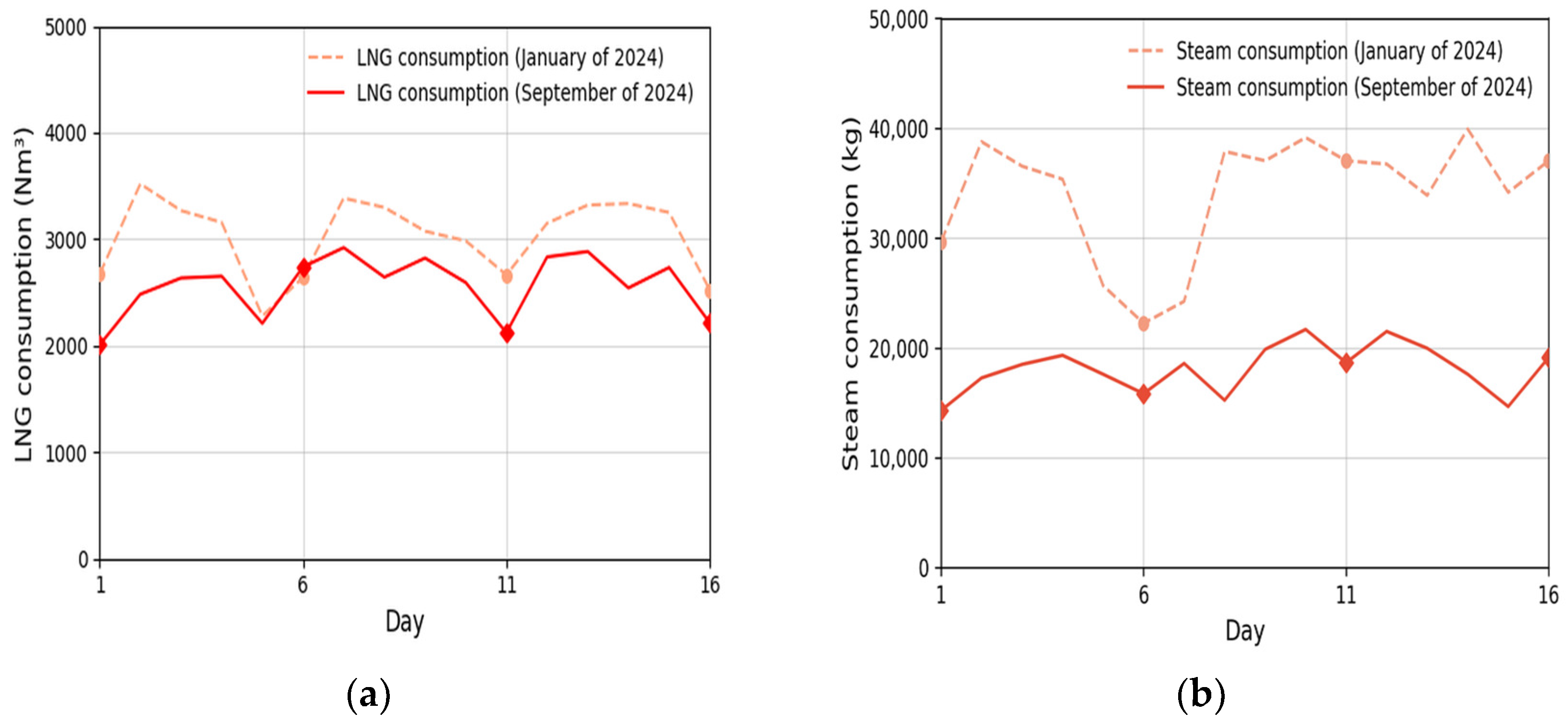
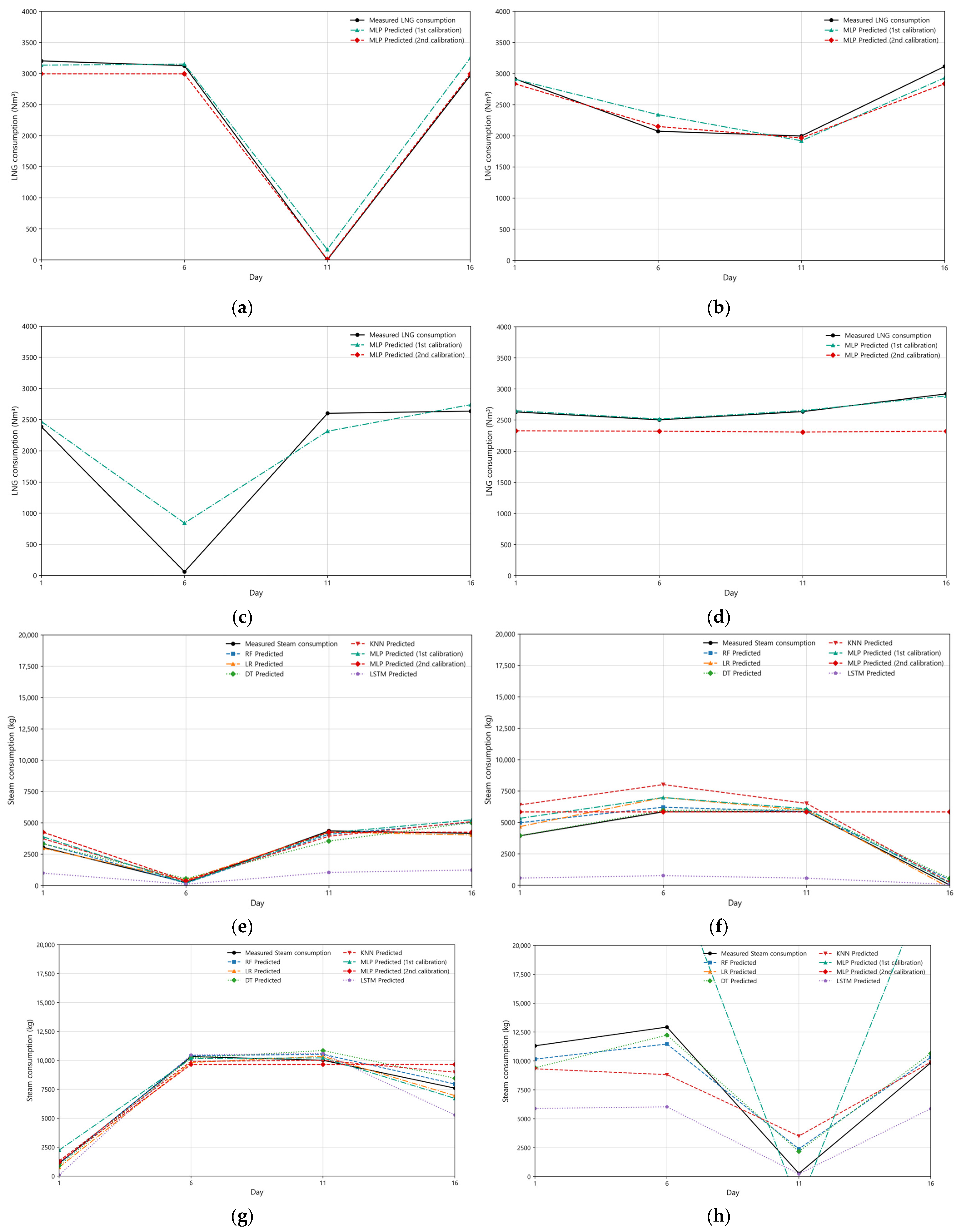
• Figure 11a: Actual LNG consumption (black solid line) starts at approximately 3200 Nm³ on the 1st day, drops to 0 Nm³ on the 11th day due to the weekend, and fluctuates around 3000 Nm³ until the 16th day. After the second calibration, the best possible prediction performance has a CVRMSE of 10.97% and an R2 of 0.9729. Detailed information is provided in Table A1 in Appendix A;
• Figure 11b: During this period, LNG consumption decreases below 3000 Nm³ before rising above 3000 Nm³. The differences are minimal; however, the second calibration results are superior according to the CVRMSE metric. Additional details are available in Table A1 in Appendix A;
• Figure 11c,d: LNG consumption predictions over the entire period highlighted significant variability influenced by operational control methods in the food factory. Initially, the MLP model struggled to capture these patterns using existing features alone. The model’s performance was found to be unsatisfactory based on the evaluation metrics, with a notably low accuracy of −60.2% and a high error rate. To overcome this, we applied k-means clustering with control mode and LNG consumption changes as features, classifying the data into three distinct operational modes, as depicted in Figure 12. The elbow method suggested an optimal (k = 4) based on inertia analysis; however, we selected (k = 3) by prioritizing domain knowledge, reflecting the three primary control methods in the food production process:

  a.

  Cluster 1: High LNG consumption during intensive production phases;

  b.

  Cluster 2: Moderate consumption under standard operating conditions;

  c.

  Cluster 3: Low consumption during reduced production or maintenance periods;

• To predict future energy consumption, we trained the MLP model on the full dataset (624 rows, including weekends) using an iterative learning approach with 30 iterations, as validated in Figure 9. This method progressively improved the model’s performance. Additionally, to evaluate the effect of irregular weekend consumption patterns, we conducted a separate analysis on a subset of 422 rows, excluding weekends. For both scenarios, we employed 5-fold time series cross-validation to ensure robustness and assess generalizability. The cross-validated performance metrics are presented below:

  1.

  With weekends (624 rows):

  a.

  MLP (1st): R² = 0.9343, CVRMSE = 18.11%, and relative accuracy = 90.86%;

  b.

  MLP (2nd): R² = −26.3140, CVRMSE = 369.59%, and relative accuracy = −86.15%;

  2.

  Excluding weekends (422 rows):

  a.

  MLP (1st): R² = 0.9855, CVRMSE = 3.99%, and relative accuracy = 98.93%;

  b.

  MLP (2nd): R² = 0.2261, CVRMSE = 49.34%, and relative accuracy = 68.62%;

• The exceptionally high performance of the initial MLP model in the weekend-excluded scenario (e.g., R² = 0.9855, accuracy = 98.93%) raised concerns about potential overfitting. However, the use of 5-fold cross-validation confirmed the model’s stability across data splits, mitigating these risks. Excluding weekends reduced noise from irregular operations, contributing to the enhanced metrics in that scenario. In contrast, the full dataset’s broader variability challenged the model, as reflected in the lower performance of the second MLP configuration. These results demonstrate the effectiveness of iterative learning in refining predictions, particularly when operational irregularities are minimized. Future work will focus on extending this approach to minute-by-minute predictions to capture finer energy consumption dynamics across the entire period.

3.2. Analysis of Steam Consumption Prediction Results

Shown in Figure 11e–h is a comparison between predicted and actual steam consumption values of the MLP model (pre- and post-hyperparameter tuning), in addition to the KNN, LR, DT, RF, and LSTM models across four processes. Although LSTM is adept at capturing long-term dependencies in time-series data, its performance declined owing to high short-term volatility and the limited sample size in this study. The following sections present a concise summary of the performance of each process based on R², CVRMSE, and relative accuracy.

3.2.1. Prediction of First Process Steam Consumption

• MLP (first): R² = 0.8766, CVRMSE = 23.46%, and relative accuracy = 80.97%. Although the CVRMSE exceeded the benchmark value, it reflects the overall trend;
• MLP (second): R² = 0.7887, CVRMSE = 30.70%, and relative accuracy = 77.72%. After performing hyperparameter tuning, the performance declined, confirming that it failed to adapt to rapid fluctuations;
• LR: R² = 0.9275, CVRMSE = 17.99%, and relative accuracy = 85.88%, demonstrating the highest performance and fulfilling the ASHRAE;
• LSTM: R² = −0.5624, CVRMSE = 83.47%, and relative accuracy = 30.68%, which failed to adapt to rapid fluctuations, resulting in the lowest performance;
• RF, DT, KNN: The overall performance metrics are stable; however, they exceed the CVRMSE threshold.

3.2.2. Prediction of Second Process Steam Consumption

• MLP (first): R² = 0.8991, CVRMSE = 14.24%, and relative accuracy = 87.87%. The performance metrics are lower than RF; however, the fluctuation patterns converged well.
• MLP (second): R² = −0.2236, CVRMSE = 49.58%, and relative accuracy = 67.90%. It failed to adapt to complex patterns, and its performance significantly deteriorated;
• RF: R² = 0.9448, CVRMSE = 10.53%, and relative accuracy = 91.27%. It demonstrates the highest performance metrics and fulfills the ASHRAE;
• LSTM: R² = −2.7628, CVRMSE = 86.94%, and relative accuracy = 20.88%. It displays a large error due to the failure to capture sudden fluctuations;
• LR, DT, KNN: The overall performance metrics are stable, but KNN exceeded the CVRMSE threshold.

3.2.3. Prediction of Third Process Steam Consumption

• MLP (first): R² = 0.8944, CVRMSE = 11.29%, and relative accuracy = 90.66%. Although these values are lower than RF, some of the altered patterns have been reflected;
• MLP (second): R² = 0.8898, CVRMSE = 11.53%, and relative accuracy = 90.13%. Its performance declined because of overestimation due to sudden fluctuations;
• RF: R² = 0.9494, CVRMSE = 7.81%, and relative accuracy = 93.93%. It demonstrated the highest performance metrics and fulfilled the ASHRAE;
• LSTM: R² = 0.5615, CVRMSE = 23.00%, and relative accuracy = 81.30%. Failure to capture pattern fluctuations and low performance metrics;
• LR, DT, KNN: The overall performance metrics are stable, however, KNN exceeded the CVRMSE standard.

3.2.4. Prediction of Fourth Process Steam Consumption

• RF: R² = 0.8981, CVRMSE = 14.10%, and relative accuracy = 90.13%. It demonstrates the highest performance metrics and satisfies the ASHRAE;
• Remaining models: Data learning failure and large errors.

4. Discussion

The results presented in Section 3 validate the effectiveness of the proposed predictive models for LNG and steam energy consumption in a food factory, fulfilling the research objectives outlined in Section 1. The LNG consumption prediction model, refined through hyperparameter tuning and k-means clustering, demonstrated a high accuracy, as detailed in Section 3.1. This precision highlights the MLP model’s capability, enhanced by adaptive control method classification, to capture complex LNG consumption patterns driven by operational variations. Such an accuracy enables real-time energy optimization in food factories, offering potential reductions in operational costs and greenhouse gas emissions. For steam consumption across the four individual processes (Section 3.2), the RF model outperformed other algorithms, consistently meeting the accuracy threshold for daily data. The RF model’s success stems from its robustness in addressing the high variability and non-linear patterns typical of process-specific steam consumption. In contrast, the LSTM model showed poor performance (e.g., a notably high CVRMSE for the second process), likely due to limited sample sizes and significant short-term volatility. This suggests that larger datasets or alternative approaches, such as hybrid models combining RF with time-series techniques (e.g., ARIMA or GRU), could better capture temporal dynamics. These findings directly support the goal of developing tailored predictive models to enhance energy efficiency within a factory energy management system (FEMS).

The RF model’s accuracy in predicting steam consumption provides precise operational insights, enabling factory operators to adjust energy inputs in real time and minimize waste. For example, optimizing steam use in heating and sterilization—key processes accounting for substantial energy consumption (Section 1.1)—can significantly reduce costs and environmental impacts. This aligns with the broader aim of mitigating the food industry’s environmental footprint, where thermal energy comprises 59% of total energy use, as noted in the 2022 statistics (Section 1.1). Unlike prior studies (e.g., [19]) that modeled aggregate LNG consumption, this study’s process-specific approach, coupled with k-means clustering to address control method variations, offers a more granular and actionable framework for the implementation of FEMSs, marking a distinct advancement in the field. The methodology’s potential extends beyond food factories to other energy-intensive sectors, such as chemical or textile industries. For instance, in chemical processing, clustering could distinguish between batch and continuous production phases, tailoring energy predictions accordingly. However, limitations remain. The LSTM model’s underperformance underscores data constraints, particularly the small sample sizes for certain processes, which restrict the use of complex time-series models. Additionally, reliance on daily aggregated data may miss minute-level fluctuations critical for finer optimization. Future research could leverage high-frequency (e.g., minute-by-minute) data and explore hybrid models like RF-LSTM or CNN-LSTM to enhance the prediction accuracy and capture short-term dynamics. Validation across diverse factory settings would further strengthen the generalizability. In summary, the proposed models provide a robust framework for energy management in food factories, with significant implications for operational efficiency and sustainability. By delivering process-specific insights and enabling real-time adjustments via a FEMS, this approach supports achieving energy efficiency targets, such as those mandated by the South Korean government (Section 1.1). These findings emphasize the value of tailored, data-driven strategies in advancing energy optimization across manufacturing sectors.

5. Conclusions

This study demonstrates that enhancing the MLP model to incorporate recent process data can achieve improved performance metrics in capturing changes in LNG consumption patterns. In the case of individual processes in food factories, a high prediction accuracy can be maintained even when simpler algorithms are applied compared to MLP. These findings provide operational guidelines for food factories lacking a FEMS, optimizing energy efficiency and subsequently lowering energy consumption. Although this model can be applied to food factories with comparable process characteristics, it requires adjustments based on each factory’s specific data attributes. Future studies will enhance the predictive model presented in this study by incorporating time- or minute-level data for more granular predictions through model improvements and by developing hybrid models that capture the unique characteristics of each process.

References

- Korea Energy Agency. 2022 Industry Sector Energy and GHG Emission Statistics; Korea Energy Agency: Ulsan, Republic of Korea, 2023; Available online: https://www.energy.or.kr/front/board/View9.do?boardMngNo=9&boardNo=24155 (accessed on 21 April 2025).
- Ministry of Trade, Industry and Energy. 3rd National Energy Basic Plan; Ministry of Trade, Industry and Energy: Sejong, Republic of Korea, 2019; Available online: https://netzero.gm.go.kr/download/%EC%A0%9C3%EC%B0%A8%20%EC%97%90%EB%84%88%EC%A7%80%EA%B8%B0%EB%B3%B8%EA%B3%84%ED%9A%8D_%EC%82%B0%EC%97%85%ED%86%B5%EC%83%81%EC%9E%90%EC%9B%90.pdf (accessed on 21 April 2025).
- Mariano-Hernández, D.; Hernández-Callejo, L.; Zorita-Lamadrid, A.; Duque-Pérez, O.; García, F.S. A review of strategies for building energy management system: Model predictive control, demand side management, optimization, and fault detect & diagnosis. J. Build. Eng. 2021, 33, 101692. [Google Scholar] [CrossRef]
- Lee, D.; Cheng, C.C. Energy savings by energy management systems: A review. Renew. Sustain. Energy Rev. 2016, 56, 760–777. [Google Scholar] [CrossRef]
- Popov, D.; Akterian, S.; Fikiin, K.; Stankov, B. Multipurpose system for cryogenic energy storage and tri-generation in a food factory: A case study of producing frozen french fries. Appl. Sci. 2021, 11, 7882. [Google Scholar] [CrossRef]
- Li, X.; Gao, J.; You, S.; Zheng, Y.; Zhang, Y.; Du, Q.; Xie, M.; Qin, Y. Optimal design and techno-economic analysis of renewable-based multi-carrier energy systems for industries: A case study of a food factory in China. Energy 2022, 244, 123174. [Google Scholar] [CrossRef]
- Hu, G.; You, F. AI-enabled cyber-physical-biological systems for smart energy management and sustainable food production in a plant factory. Appl. Energy 2024, 356, 122334. [Google Scholar] [CrossRef]
- Jagtap, S.; Rahimifard, S.; Duong, L.N. Real-time data collection to improve energy efficiency: A case study of food manufacturer. J. Food Process Preserv. 2022, 46, e14338. [Google Scholar] [CrossRef]
- Al Momani, D.; Al Turk, Y.; Abuashour, M.I.; Khalid, H.M.; Muyeen, S.; Sweidan, T.O.; Said, Z.; Hasanuzzaman, M. Energy saving potential analysis applying factory scale energy audit—A case study of food production. Heliyon 2023, 9, e14216. [Google Scholar] [CrossRef]
- Geng, D.; Evans, S.; Kishita, Y. The identification and classification of energy waste for efficient energy supervision in manufacturing factories. Renew. Sustain. Energy Rev. 2023, 182, 113409. [Google Scholar] [CrossRef]
- Munguia, N.; Velazquez, L.; Bustamante, T.P.; Perez, R.; Winter, J.; Will, M.; Delakowitz, B. Energy audit in the meat processing industry—A case study in Hermosillo, Sonora Mexico. J. Environ. Prot. 2016, 7, 14–22. [Google Scholar] [CrossRef]
- Tanaka, K.; Managi, S. Industrial agglomeration effect for energy efficiency in Japanese production plants. Energy Policy 2021, 156, 112442. [Google Scholar] [CrossRef]
- Kluczek, A.; Olszewski, P. Energy audits in industrial processes. J. Clean. Prod. 2017, 142, 3437–3453. [Google Scholar] [CrossRef]
- Walther, J.; Weigold, M. A systematic review on predicting and forecasting the electrical energy consumption in the manufacturing industry. Energies 2021, 14, 968. [Google Scholar] [CrossRef]
- Bermeo-Ayerbe, M.A.; Ocampo-Martinez, C.; Diaz-Rozo, J. Data-driven energy prediction modeling for both energy efficiency and maintenance in smart manufacturing systems. Energy 2022, 238, 121691. [Google Scholar] [CrossRef]
- Kapp, S.; Choi, J.K.; Hong, T. Predicting industrial building energy consumption with statistical and machine-learning models informed by physical system parameters. Renew. Sustain. Energy Rev. 2023, 172, 113045. [Google Scholar] [CrossRef]
- Corigliano, O.; Aligieri, A. A comprehensive investigation on energy consumptions, impacts, and challenges of the food industry. Energy Convers. Manage. X 2024, 23, 100661. [Google Scholar] [CrossRef]
- Ladha-Sabur, A.; Bakalis, S.; Fryer, P.J.; Lopez-Quiroga, E. Mapping energy consumption in food manufacturing. Trends Food Sci. Technol. 2019, 86, 270–280. [Google Scholar] [CrossRef]
- Lee, H.; Kim, D.; Gu, J.H. Prediction of food factory energy consumption using MLP and SVR algorithms. Energies 2023, 16, 1550. [Google Scholar] [CrossRef]
- ASHRAE. ASHRAE Guideline 14-2014: Measurement of Energy Demand and Savings; American Society of Heating, Refrigerating and Air-Conditioning Engineers: Atlanta, GA, USA, 2014; Available online: https://scholar.google.com/scholar_lookup?title=Measurement%20of%20Energy%20and%20Demand%20Savings&author=ASHRAE%2C%20ASHRAE%20Guideline%2014-2014&publication_year=2014 (accessed on 21 April 2025).
- Webster, L.J.; Bradford, J. M&V Guidelines: Measurement and Verification for Federal Energy Projects, Version 5.0. Technical Report; U.S. Department of Energy Federal Energy Management Program: Washington, DC, USA, 2015. Available online: https://www.energy.gov/sites/prod/files/2016/01/f28/mv_guide_4_0.pdf (accessed on 21 April 2025).
- Schreiber, J.; Sick, B. Model selection, adaptation, and combination for transfer learning in wind and photovoltaic power forecasts. Energy AI 2023, 14, 100249. [Google Scholar] [CrossRef]
- Berrisch, J.; Narajewski, M.; Ziel, F. High-resolution peak demand estimation using generalized additive models and deep neural networks. Energy AI 2023, 13, 100236. [Google Scholar] [CrossRef]
- Ansar, T.; Ashraf, W.M. Comparison of Kolmogorov–Arnold Networks and Multi-Layer Perceptron for modelling and optimisation analysis of energy systems. Energy AI 2025, 20, 100473. [Google Scholar] [CrossRef]
- Radaideh, M.I.; Rigopoulos, S.; Goussis, D.A. Characteristic time scale as optimal input in Machine Learning algorithms: Homogeneous autoignition. Energy AI 2023, 14, 100273. [Google Scholar] [CrossRef]
- Piantadosi, G.; Dutto, S.; Galli, A.; De Vito, S.; Sansone, C.; Di Francia, G. Photovoltaic power forecasting: A Transformer based framework. Energy AI 2024, 18, 100444. [Google Scholar] [CrossRef]