An Unsupervised Anomaly Detection Method for Nuclear Reactor Coolant Pumps Based on Kernel Self-Organizing Map and Bayesian Posterior Inference

Abstract

Effectively monitoring the operational status of reactor coolant pumps (RCPs) is crucial for enhancing the safety and stability of nuclear power operations. To address the challenges of limited interpretability and suboptimal detection performance in existing methods for detecting abnormal operating states of RCPs, this paper proposes an interpretable, unsupervised anomaly detection approach. This innovative method designs a framework that combines Kernel Self-Organizing Map (Kernel SOM) clustering with Bayesian Posterior Inference. Specifically, the proposed method uses Kernel SOM to extract typical patterns from normal operation data. Subsequently, a distance probability distribution model reflecting the data distribution structure within each cluster is constructed, providing a robust tool for data distribution analysis for anomaly detection. Finally, based on prior knowledge, such as distance probability distribution, the Bayesian Posterior Inference is employed to infer the probability of the equipment being in a normal state. By constructing distribution models that reflect data distribution structures and combining them with posterior inference, this approach realizes the traceability and interpretability of the anomaly detection process, improving the transparency of anomaly detection and enabling operators to understand the decision logic and the analysis of the causes of anomalous occurrences. Verification via real-world operational data demonstrates the method’s superior effectiveness. This work offers a highly interpretable solution for RCP anomaly detection, with significant implications for safety-critical applications in the nuclear energy sector.

1. Introduction

The safety of nuclear power plants (NPPs) is increasingly critical due to advances in nuclear technology and equipment complexity. Among the key components, reactor coolant pumps (RCPs) are essential for transferring energy within the coolant system, ensuring stable NPP operation [1]. However, RCPs usually operate for a long time under extreme conditions (high temperatures and high pressure), making them susceptible to degradation from corrosion and wear [2]. This vulnerability has led to over 100 documented anomaly-induced shutdowns and maintenance events, imposing significant financial burdens on operators [3,4]. RCPs consist of many complex components, the monitored data of which are complex and diverse, posing challenges and becoming an error-prone problem for operators to manually detect anomalous states from a large amount of sensor data through preset thresholds. Consequently, timely and accurate automatic anomaly detection is crucial for enhancing RCP maintenance and operational reliability, mitigating the risk of severe accidents and economic losses.

Current approaches to anomaly detection in nuclear power equipment are categorized into two primary types: supervised and unsupervised algorithms. Supervised algorithms have gained considerable traction and include techniques such as logistic regression [5], K-Nearest Neighbors (KNNs) [6], Support Vector Machines (SVM) [7,8], Broad Learning Systems (BLSs) [9], and Artificial Neural Networks (ANNs) [10,11,12]. Within the domain of RCP anomaly detection, supervised techniques have demonstrated significant potential. For instance, Wang et al. [13] proposed a BLS-based model characterized by a simple network structure and a step-by-step learning approach, which effectively detects coolant leaks with high accuracy. Additionally, convolutional neural networks (CNNs), a type of ANN, are recognized for their ability to automatically identify important patterns within complex data. Yang et al. [14] transformed fault signals into Symmetrized Dot Pattern (SDP) images, using a depthwise separable CNN to effectively diagnose coolant system faults. Similarly, Zhang et al. [15] developed a hybrid 1D–2D CNN framework enhanced by Neural Architecture Search, which autonomously optimizes hyperparameters to deliver robust solutions for RCP leak detection and fault diagnosis.

Despite their strengths, supervised methods encounter substantial challenges in anomaly detection of NPP equipment. Due to strict maintenance and inspection measures, the anomalies happen at a far lower frequency than the normal working states in NPPs, and a large number of abnormal samples cannot be provided for supervised methods. In addition, in most cases, NPP accidents are characterized by occasional symptoms, and there are a large number of unlabeled anomalies. It is difficult for supervised methods to identify these unlabeled anomalies. These shortcomings restrict their practical application for RCP monitoring.

In contrast, unsupervised algorithms eliminate the need for labeled data entirely. Classical algorithms such as K-means clustering and Principal Component Analysis (PCA) uncover latent data structures and patterns through distance metrics or linear transformations. However, early unsupervised methods were constrained by their reliance on oversimplified distributional assumptions, exhibiting limited ability in high-dimensional structured datasets. In recent years, unsupervised methods based on neural networks (e.g., Self-Organizing Map (SOM) [16,17] and Autoencoder (AE) [18]) have achieved representation learning of complex features through hierarchical learning and have been widely applied in industrial anomaly detection. For instance, the SOM method, due to its powerful capabilities in local patterns analysis and visualization, has been widely applied in anomaly detection across various industrial fields, including power systems [19], petroleum [20], and maritime engineering [21].

In the field of NPP anomaly detection, specifically in the field of RCP anomaly detection, the current research primarily focuses on critical scenarios like coolant loss. For instance, Cancemi et al. [22] addressed data scarcity in coolant loss events by training an AE model exclusively on normal operational data and detecting anomalies through reconstruction error thresholds. Similarly, Li et al. [23] tackled the lack of transient anomaly data by integrating the Variational Autoencoder (VAE) with the Isolation Forest (iForest) algorithm, developing a VAE + iForest model that achieved high-precision detection of RCP anomalies. Furthermore, Sun et al. [24] proposed a Convolutional Adversarial Autoencoder with Self-Attention (CAAE-SA) to mitigate noise interference in NPP monitoring signals. By employing attention-driven feature weighting, this architecture demonstrated superior performance in diagnosing coolant leakage, oil tank failures, and third-stage shaft seal degradation. Although these deep learning-based methods have achieved remarkable detection accuracy for RCP anomalies, their reliance on deep neural networks introduces new challenges. The black-box nature of deep neural networks makes it difficult to trace the logical relationship between inputs and outputs. This results in opaque decision-making processes and limited interpretability, severely hampering operators’ ability to comprehend anomaly detection criteria and judge decision reliability. It may lead to distrust and misunderstanding of the output results from the anomaly monitoring models by the operators, potentially bringing adverse effects to the safety of NPPs.

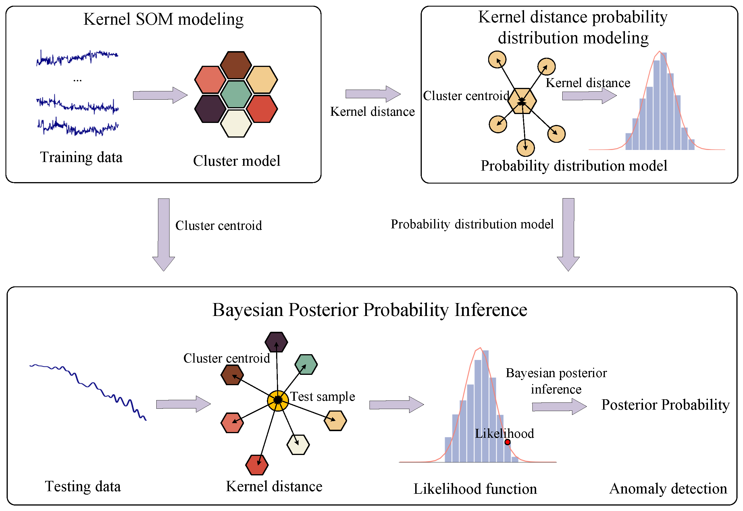
To address these challenges, in this article, we aim to develop an excellent performance and interpretable method for RCP anomaly detection. To this end, this paper designs an unsupervised anomaly detection framework and validates it with real-world monitoring data of an RCP of an NPP. The framework consists of three key components: clustering, distance probabilistic distribution modeling, and Bayesian Posterior Inference. The clustering module is responsible for extracting typical patterns of normal-state data. Distance probability distribution modeling provides prior information on probability distribution for Bayesian Posterior Inference by describing the distribution patterns of data in each cluster from clustering. It acts as a bridge between the clustering module and the Bayesian Posterior Inference module. Finally, sample kernel distances and prior knowledge of distance probability distributions are input into the Bayesian Posterior Inference module to estimate the probability of a sample being normal. In the clustering process, the model needs to thoroughly capture local patterns and features of the normal state to construct a clustering model that effectively represents different subcategories of normal conditions. The Kernel Self-Organizing Map (Kernel SOM) network has a strong ability to extract local patterns and features. Compared to classic SOM, it is more suitable for analyzing nonlinear data. Thus, it is highly suitable for this research. Therefore, the Kernel SOM algorithm has been adopted as the clustering method in this work.

In conclusion, our main contributions are as follows:

• A novel anomaly monitoring method for RCPs has been proposed in this paper. To the best of our knowledge, this is the first attempt to analyze the distribution of normal-state data by constructing a probabilistic distribution model and integrating it with posterior inference to construct an anomaly monitoring model for identifying RCP abnormal events.
• The method designs a distance probability distribution model that reflects the data distribution. By constructing a distance-based probability distribution model for each clustering cluster, we can directly compare the differences in distance distribution between abnormal and normal data, which helps operators understand the basis for anomaly judgment.
• The method designs a traceable anomaly detection framework. By combining the distance distribution model and other prior knowledge with Bayesian Posterior Inference, the proposed method achieves traceability in anomaly detection decisions. This allows operators to trace the detection results and identify the root causes of differences between abnormal and normal states.
• The proposed method was compared with other anomaly detection methods based on monitoring data of RCP anomalies from NPPs. The results demonstrated the superiority of our approach. We believe this generalizable anomaly detection method can be applied to other equipment in NPPs.

The following sections are structured in the following manner: Section 2 introduces the relevant theories and methods. Section 3 provides a detailed description of the proposed method. Section 4 discusses the performance and interpretability of the proposed method. Section 5 concludes with an overview of the findings and future research directions.

2. Related Theories

In this section, the principles of the Self-organizing Map (SOM) and its extension, the Kernel SOM network, will be introduced.

2.1. SOM

SOM is a competitive learning-based unsupervised neural network. Its core mechanism involves iterating to find the Best Matching Unit (BMU) and adjusting neighboring unit weights, which enables SOM to identify local data patterns and structures and detect subtle data differences. The learning process of SOM can be summarized as follows.

For an input sample ${\mathbf{f}}_t$ at iteration t, the BMU ${\mathbf{c}}_i$ is determined by minimizing the Euclidean distance:

$$j=\mathrm{argmin}d[{\mathbf{f}}_t,{\mathbf{c}}_i],$$

(1)

where $d(·)$ represents the Euclidean distance. When the BMU is found, the BMU and its topological neighbors will update their weight vectors according to

$$\left\{\begin{array}{c}{\mathbf{c}}_i(t+1)={\mathbf{c}}_i\left(t\right)+\gamma \left(t\right)h_{ci}\left(t\right)[{\mathbf{f}}_t-{\mathbf{c}}_i\left(t\right)],i\in N_j\left(t\right)\hfill \\ {\mathbf{c}}_i(t+1)={\mathbf{c}}_i\left(t\right),i\notin N_j\left(t\right)\hfill \end{array}\right.,$$

(2)

where t represents the update iteration, $\gamma \left(t\right)$ is the learning rate (between 0 and 1, decreasing monotonically with time), and $N_j\left(t\right)$ defines the neighborhood around BMU $c_j$ at iteration t. The neighborhood function $h_{ci}(·)$ defines the weight update intensity for nodes in the neighborhood of the BMU, ensuring that closer neurons are updated more strongly to preserve topological relationships:

$$h_{ci}\left(t\right)=\exp ({\displaystyle \frac{-d_{ci}^2}{2\sigma {\left(t\right)}^2}})$$

(3)

where $d_{ci}$ is the distance between the BMU and the i-th neuron, and $\sigma \left(t\right)$ is the neighborhood radius that changes over time.

2.2. Kernel SOM

Traditional SOM struggles with nonlinear data distributions and capturing feature relationships in high-dimensional data due to its reliance on Euclidean distance, a limitation particularly evident in complex systems like RCPs. To address these shortcomings, Kernel SOM [25] introduces kernel functions [26], replacing Euclidean distance with kernel distance. This implicitly maps data to a high-dimensional feature space, enabling more effective similarity calculations and capturing nonlinear relationships. Common choices for the kernel function $K(·)$ include the Gaussian kernel and polynomial kernel, which enhance the model’s ability to handle nonlinear data structures. The kernel distance is calculated as

$$d_k({\mathbf{f}}_t,c_i)=K({\mathbf{f}}_t,{\mathbf{f}}_t)-2K({\mathbf{f}}_t,{\mathbf{c}}_i)+K({\mathbf{c}}_i,{\mathbf{c}}_i),$$

(4)

where $K(·,·)$ represents the kernel function. The weight update in Kernel SOM is performed in the feature space using the gradients of the kernel function:

$$\left\{\begin{array}{c}{\mathbf{c}}_i(t+1)={\mathbf{c}}_i\left(t\right)+\gamma \left(t\right)h_{ci}\left(t\right)[{\displaystyle \frac{\partial K({\mathbf{c}}_i,{\mathbf{c}}_i)}{\partial {\mathbf{c}}_i}}-2{\displaystyle \frac{\partial K({\mathbf{f}}_t,{\mathbf{c}}_i)}{\partial {\mathbf{c}}_i}}],i\in N_j\left(t\right)\hfill \\ {\mathbf{c}}_i(t+1)={\mathbf{c}}_i\left(t\right),i\notin N_j\left(t\right)\hfill \end{array}\right..$$

(5)

By leveraging these gradients, Kernel SOM adjusts the weights in the high-dimensional feature space, effectively learning nonlinear mappings. Thus, it is especially suitable for anomaly detection in complex, nonlinear systems.

Although Kernel SOM improves the SOM algorithm’s ability to handle nonlinear data, anomaly detection methods based on Kernel SOM still face numerous challenges. For instance, the anomaly detection mechanism of Kernel SOM relies merely on whether the distance exceeds a predefined threshold to identify anomalies [27], which is a relatively simplistic approach and, thus, prone to misjudgments. Moreover, due to the lack of an interpretability mechanism, Kernel SOM cannot directly provide a reliable internal logic for anomaly detection. In this paper, we creatively propose a framework that integrates the Kernel SOM and the distance probability distribution model with Bayesian Posterior Inference. First, the distribution model is used to analyze the patterns of clustered data points. Then, Bayesian Posterior Inference is employed to accurately estimate the probability of samples being normal. Thereby, the proposed approach mitigates misjudgments in anomaly detection while constructing a highly interpretable anomaly detection model.

3. Methodology

In this section, the core components of the proposed unsupervised anomaly detection method are discussed. An anomaly is defined as a data point whose similarity to established normal patterns falls below a threshold determined through statistical analysis [28]. The proposed framework quantifies the similarity between observed objects and normal states, consisting of three primary modules: Kernel SOM Clustering, Kernel Distance Probability Distribution Modeling, and Bayesian Posterior Probability Inference. These modules are illustrated in Figure 1. The functional roles of each module are described below:

• Kernel SOM Clustering: Groups normal data into clusters to identify typical operational patterns.
• Kernel Distance Probability Distribution Modeling: Models the statistical distribution of kernel distances between normal samples and cluster centroids to define normal behavior.
• Bayesian Posterior Probability Inference: Combines prior knowledge from distance models with real-time data to compute the posterior probability that a sample belongs to the normal class and identify anomalous instances.

3.1. Kernel Distance Probability Distribution Modeling

Using the clusters generated by Kernel SOM, a kernel distance probability distribution model for each cluster has been constructed to capture the statistical distribution patterns of distances between normal samples and their respective cluster centroids. These models define probabilistic baselines for normal operation, establishing the expected range and distribution of kernel distances within each cluster. Anomalous samples are flagged if their distance deviates significantly from the expected range, thus improving detection interpretability and enabling operators to visually assess the alignment between test samples and normal distributions.

Let the clusters from Kernel SOM be denoted as $C=\{C_1,C_2,\dots ,C_m\}$, with corresponding centroids $c=\{c_1,c_2,\dots ,c_m\}$, where m is the number of clusters. For a given cluster $C_i$, the kernel distances between its normal samples and the centroid $c_i$ are denoted as $D_i=\{d_{i,1},d_{i,2},\dots ,d_{i,n_i}\}$, where $n_i$ is the number of samples in $C_i$. Considering the influence of the kernel SOM clustering learning mechanism, the distribution of distances within each cluster exhibits morphological characteristics similar to a Gaussian distribution. Therefore, this paper assumes that the Gaussian distribution is followed:

$$D_i\sim N({\mu }_i,{\sigma }_i^2).$$

(6)

To estimate the parameters ${\mu }_i$ and ${\sigma }_i^2$, we define the likelihood function $L({\mu }_i,{\sigma }_i^2)$ for the Gaussian probability density:

$$L({\mu }_i,{\sigma }_i^2)=\prod _{k=1}^{n_i}{\displaystyle \frac{1}{\sqrt{2\pi {\sigma }_i^2}}}exp\left(-{\displaystyle \frac{{(d_{i,k}-{\mu }_i)}^2}{2{\sigma }_i^2}}\right),$$

(7)

where $d_{i,k}$ is the kernel distance between the k-th sample in $D_i$ and $c_i$. When taking the natural logarithm to facilitate maximization,

$$lnL({\mu }_i,{\sigma }_i^2)=-{\displaystyle \frac{n_i}{2}}ln\left(2\pi \right)-{\displaystyle \frac{n_i}{2}}ln\left({\sigma }_i^2\right)-{\displaystyle \frac{1}{2{\sigma }_i^2}}\sum _{k=1}^{n_i}{(d_{i,k}-{\mu }_i)}^2$$

(8)

By computing the partial derivatives with respect to ${\mu }_i$ and ${\sigma }_i^2$ and setting them to zero, we obtain the maximum likelihood estimates:

$$\left\{\begin{array}{c}{\mu }_i={\displaystyle \frac{1}{n_i}}{\displaystyle \sum _{k=1}^{n_i}}{d}_{i,k}\hfill \\ {\sigma }_i^2={\displaystyle \frac{1}{n_i}}{\displaystyle \sum _{k=1}^{n_i}}{(d_{i,k}-{\mu }_i)}^2\hfill \end{array}\right.$$

(9)

3.2. Bayesian Posterior Probability Inference

The Bayesian Posterior Inference is used to assess the match between an observed sample and the normal patterns defined by the distance models. Specifically, the posterior probability of a sample belonging to a particular cluster is computed by integrating prior knowledge (e.g., the distance probability distribution) with real-time data. This probabilistic framework facilitates the interpretation of anomaly detection by providing a quantitative measure of how closely a sample aligns with normal operational patterns. The detailed procedure for posterior probability inference is as follows.

Posterior Probability Inference. Let $d_{si}$ denote the kernel distance between a given sample s and the centroid $c_i$ of cluster $C_i$. According to Bayes’ theorem, the posterior probability that s belongs to cluster $C_i$, denoted as $P\left(C_i\right|d_{si})$, is given by

$$P\left(C_i\right|d_{si})={\displaystyle \frac{P\left(d_{si}\right|C_i)P\left(C_i\right)}{P\left(d_{si}\right)}}={\displaystyle \frac{P\left(d_{si}\right|C_i)P\left(C_i\right)}{{\displaystyle \sum _{j=1}^m}P\left(d_{si}\right|C_j)P\left(C_j\right)}}.$$

(10)

here, $P\left(C_i\right|d_{si})$ represents the likelihood function, which is defined by the Gaussian distribution in Equation (6), and $P\left(C_i\right)$ is the prior probability of a sample belonging to cluster $C_i$, calculated as

$$P\left(C_i\right)={\displaystyle \frac{N_i}{N}}$$

(11)

where $N_i$ is the number of samples assigned to $C_i$, and N is the total number of samples in the training dataset.

Anomaly Judgment. The posterior probabilities of a sample s belonging to each cluster are calculated. The maximum of these probabilities is selected as the likelihood that the sample s is normal:

$$P_{normal}=max(P\left(C_i\right|d_{s1}),P\left(C_i\right|d_{s2}),\dots ,P\left(C_i\right|d_{sm}))$$

(12)

To establish a threshold for distinguishing between normal and abnormal conditions, we use the $3\sigma$ rule [29]. This rule applies to the posterior probabilities of normal samples from the training phase to calculate a threshold value:

$$P_{th}={\mu }_p-3{\sigma }_p$$

(13)

where $P_{th}$ is the decision threshold, and ${\mu }_p$ and ${\sigma }_p$ represent the mean and variance of the posterior probabilities of normal samples during the training phase, respectively. If $P_{\mathrm{normal}}$ exceeds $P_{th}$, the sample is classified as normal; otherwise, it is deemed anomalous.

4. Verification and Analysis

In this section, we validate the effectiveness of the proposed method using pressure monitoring data from the mechanical seals of an RCP. By comparing the proposed method with Kernel SOM, we demonstrate the improvement in Kernel SOM performance through probability distribution modeling and posterior inference. The described verification process includes dataset description, feature analysis, modeling, and evaluation. The dataset description elaborates on the sampling process and results of the verification data used. Feature analysis extracted appropriate features based on the differences between the normal and abnormal states of the verification data, which are then fed into the anomaly detection model. Modeling and evaluation completed the selection of hyperparameters during the construction process of the proposed anomaly detection method and verified the effectiveness of the model.

4.1. Evaluation Metrics

To evaluate the performance of the proposed anomaly detection method, the F1-score, a commonly employed metric that balances precision and recall, is used in this paper. Precision represents the proportion of correctly detected anomalies among all detected anomalies. A higher precision indicates fewer false positives. Recall represents the proportion of correctly detected anomalies among all actual anomalies. A higher recall indicates fewer false negatives. The formulas for precision, recall, and F1-score are presented in Equation (14):

$$\begin{array}{cc}\hfill \mathrm{Precision}& ={\displaystyle \frac{TP}{TP+FP}}\hfill \\ \hfill \mathrm{Recall}& ={\displaystyle \frac{TP}{TP+FN}}\hfill \\ \hfill \mathrm{F}1\text{-}\mathrm{score}& =2·{\displaystyle \frac{\mathrm{Precision}·\mathrm{Recall}}{\mathrm{Precision}+\mathrm{Recall}}}\hfill \end{array}$$

(14)

in these formulas, TP (True Positive) represents the number of anomalies correctly detected as anomalies, FP (False Positive) represents the number of normal instances incorrectly detected as anomalies, and FN (False Negative) represents the number of anomalies incorrectly classified as normal.

In addition to these traditional metrics, considering the importance of timely anomaly alarms in NPP equipment monitoring, lag time is introduced as a measure of the timeliness of anomaly detection. This indicator is defined as the difference between the alarm trigger time and the actual occurrence time of the anomaly, providing a measure of the model’s responsiveness.

4.2. Dataset and Preprocessing

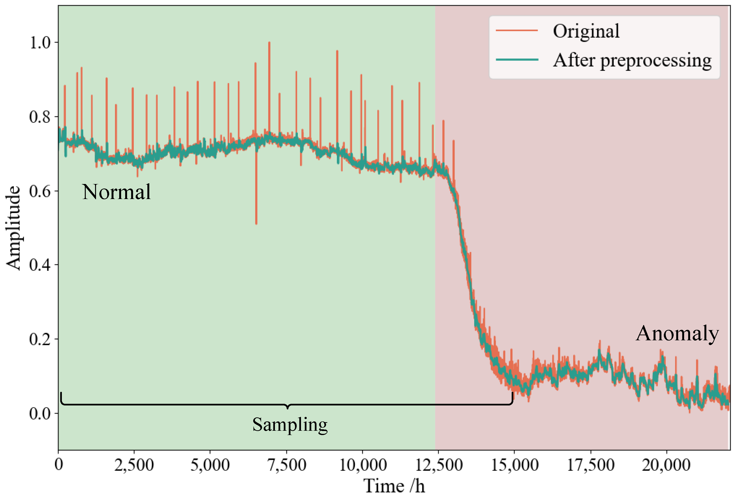
The dataset used in this study consists of pressure monitoring data from the mechanical seal of an RCP of an NPP. The monitoring period spans approximately 22,400 h. As illustrated in Figure 2, when the monitored pressure deviates from the normal range and exhibits a gradual downward trend, it indicates potential leakage failure in the mechanical seal of the RCP. Based on this observation, we classify the dataset into normal and abnormal states and sample separately for preprocessing. Data preprocessing involved sampling the data with a sliding window method, where the window size is 5 h, and the step size is 1 h. For abnormal data, we specifically selected the falling-edge segments, periods where the pressure begins to decline, to capture the most relevant anomaly data. Finally, as summarized in

Table 1. The information of the verification data.

Accident Types	Number of Samples	Number of Training Samples	Number of Testing Samples
Normal	11,925	10,000	1925
Anomaly	1965	0	1965

, the normal samples were divided into training and test sets, while all the abnormal samples were used for testing.

4.3. Feature Analysis

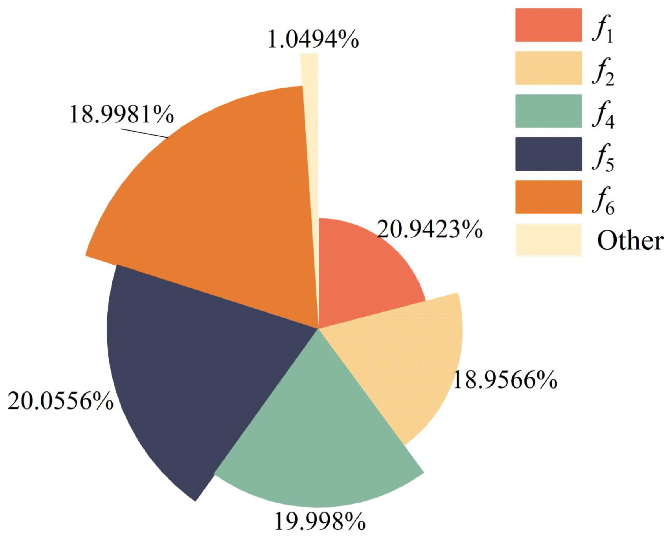
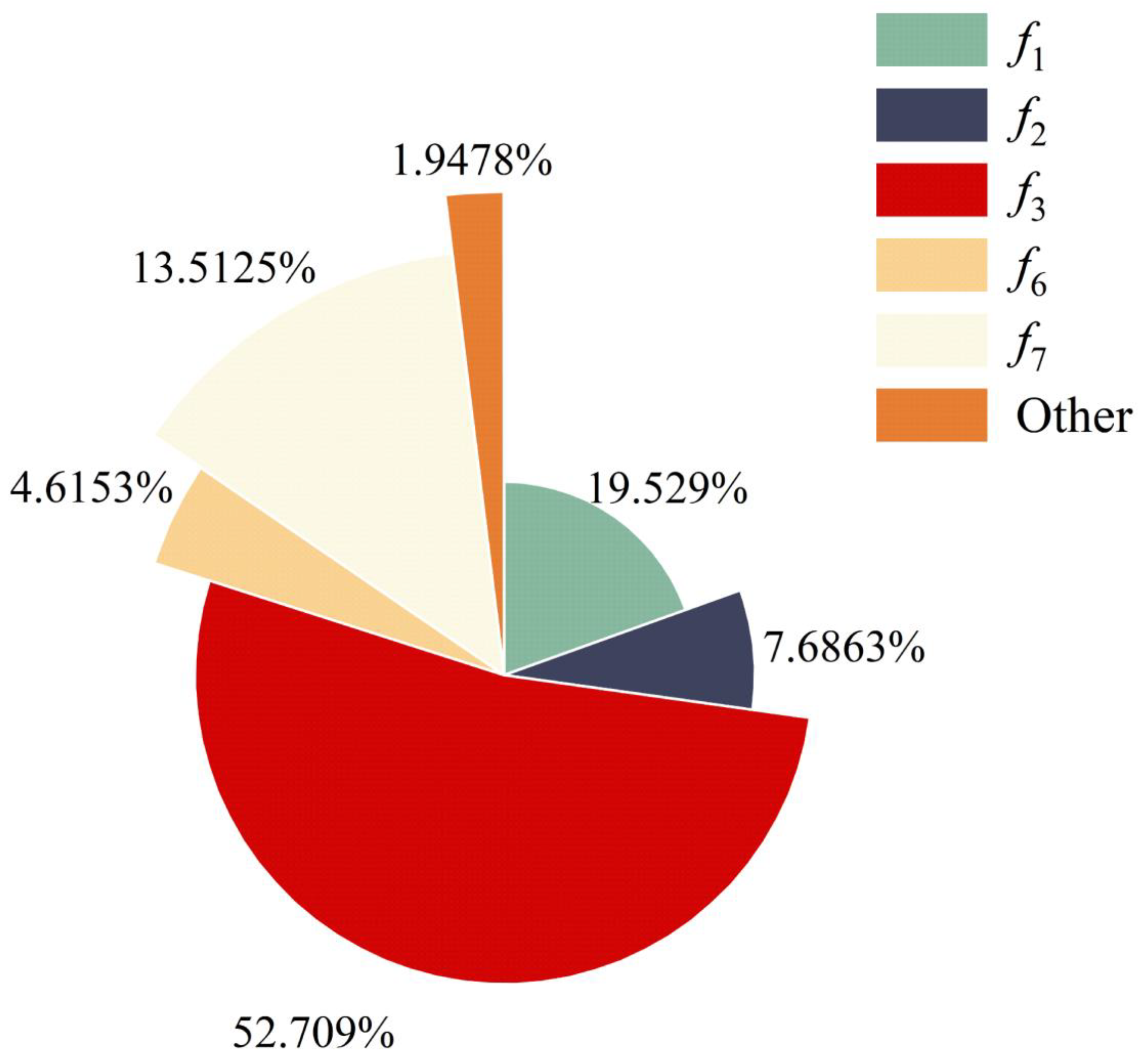
When a mechanical seal failure occurs, the monitored pressure values gradually decrease, resulting in deviations from normal operating ranges. This deviation results in distinguishable differences in both time-domain and frequency-domain statistical characteristics between normal and abnormal signals. To characterize these anomalies systematically, we conducted a joint time-frequency analysis of the monitoring signals and extracted the relevant features.

The time-domain features extracted from the pressure signals are summarized in

Table 2. The time domain features.

NO.	Features	Formula	NO.	Features	Formula
$f_1$	Max	$x_{max}=\max (x_1,x_2,\dots ,x_l)$	$f_2$	Min	$x_{min}=\min (x_1,x_2,\dots ,x_l)$
$f_3$	Range	$x_r=x_{max}-x_{min}$	$f_4$	Mean	$x_{mean}={\displaystyle \frac{1}{l}}{\sum }_{i=1}^l{x}_i$
$f_5$	Slope	$x_{slope}={\displaystyle \frac{x_{max}-x_{min}}{l}}$	$f_6$	RMS	$x_{rms}=\sqrt{{\displaystyle \frac{1}{l}}{\sum }_{i=1}^l{x}_i^2}$
$f_7$	Skewness	$x_{sk}={\displaystyle \frac{1}{l}}{\sum }_{i=1}^l{\left({\displaystyle \frac{x_i-\overline{x}}{\sigma }}\right)}^3$	$f_8$	Kurtosis	$x_k={\displaystyle \frac{1}{l}}{\sum }_{i=1}^l{\left({\displaystyle \frac{x_i-\overline{x}}{\sigma }}\right)}^4$

where l is the length of the signal.

. These features capture various aspects of the signal, such as the maximum (Max), minimum (Min), range, mean, slope, root mean square (RMS), skewness, and kurtosis. In addition to time-domain features, frequency-domain features were extracted to capture the signal’s frequency characteristics. The frequency-domain features, including frequency center, root mean square frequency, and variance frequency, are summarized in

Table 3. The frequency domain features.

NO.	Features	Formula
$f_9$	Frequency center	$x_{fc}={\displaystyle \frac{{\sum }_{i=1}^m{f}_{i}P\left(i\right)}{{\sum }_{i=1}^{m}P\left(f_i\right)}}$
$f_{10}$	Root mean square frequency	$x_{rmsf}=\sqrt{{\displaystyle \frac{{\sum }_{i=1}^m{f}_i^{2}P\left(i\right)}{{\sum }_{i=1}^{m}P\left(f_i\right)}}}$
$f_{11}$	Variance frequency	$x_{vf}=\sqrt{{\displaystyle \frac{{\sum }_{i=1}^m{(f_i-x_{fc})}^{2}P\left(i\right)}{{\sum }_{i=1}^{m}P\left(f_i\right)}}}$

where $P\left(i\right)$ is the i-th value of the frequency spectrum, m is the number of spectrum lines, and $f\left(i\right)$ is the frequency of the i-th spectrum line.

.

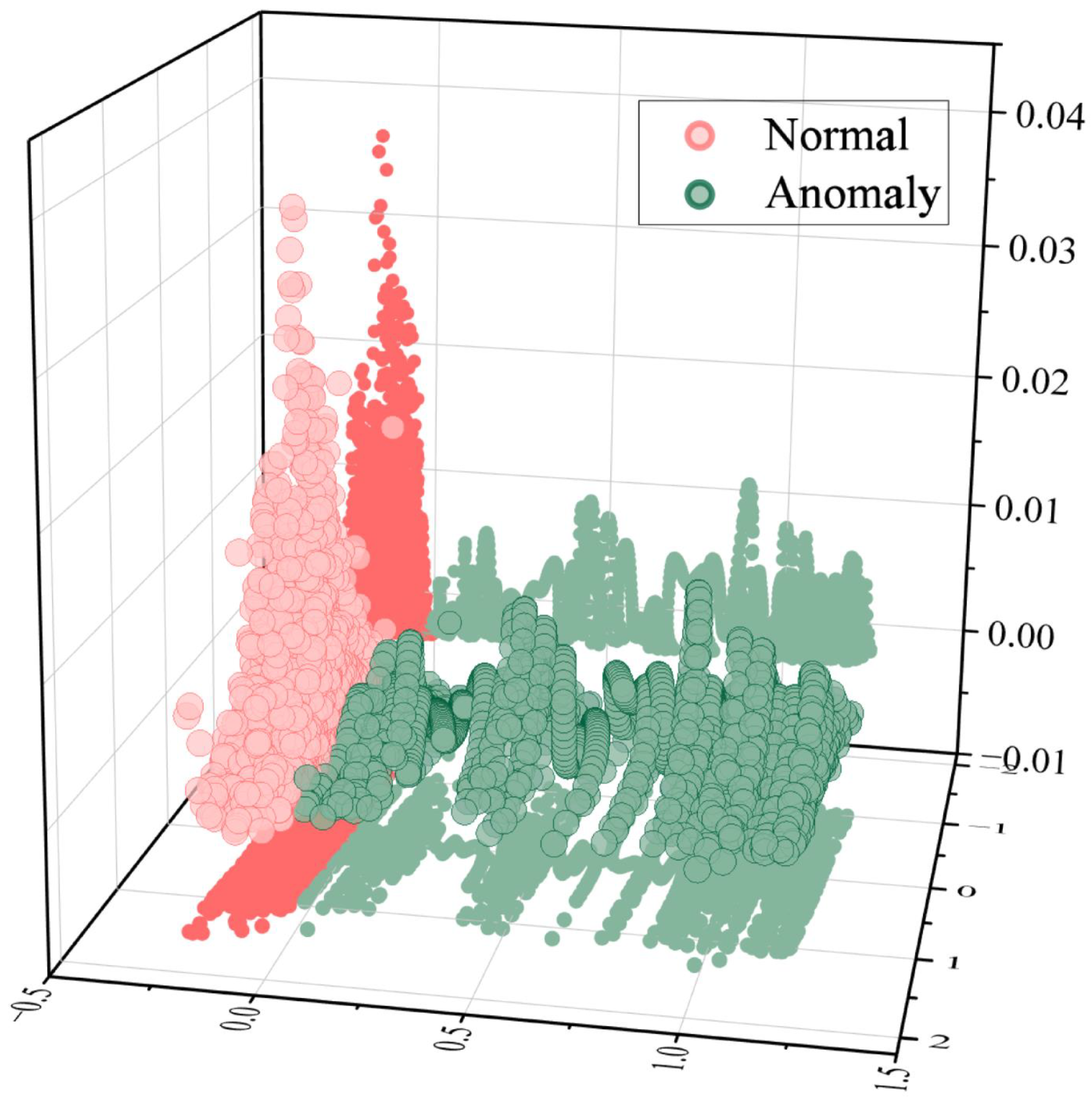
To evaluate the discriminative power of the proposed features across different operational states, the feature distributions under normal and abnormal conditions have been visualized, as illustrated in Figure 3. It is important to note that, to facilitate visualization, Principal Component Analysis (PCA) was applied to reduce the dimensionality of the extracted features. As illustrated in Figure 3, normal-state data exhibit a high concentration distribution in the dimensionality-reduced space, reflecting high feature similarity under normal operating conditions. In contrast, abnormal-state data display dispersed distributions with a distinct boundary separating them from normal data. This pronounced divergence confirms that abnormal features significantly differ from normal ones, demonstrating that the proposed features effectively capture discriminative characteristics between operational states.

4.4. Modeling and Evaluation

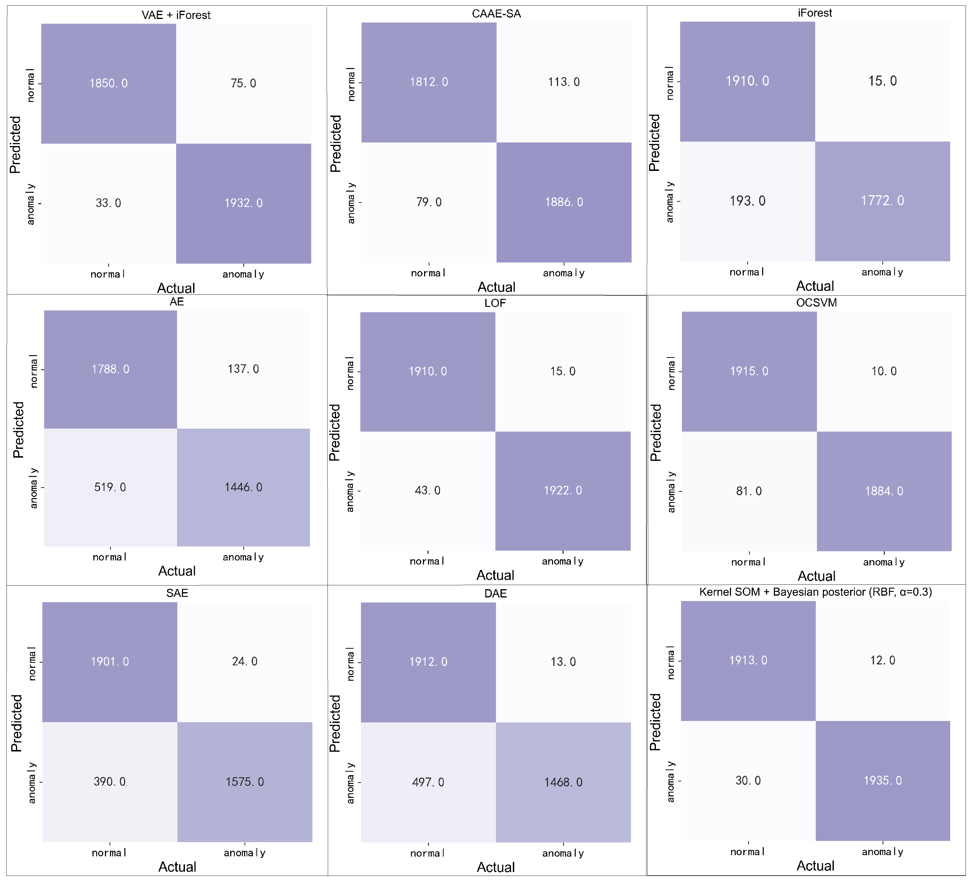
Given the significant impact of Kernel SOM network size and Kernel function type on model performance, we conducted grid search experiments to explore the performance of the Kernel SOM + Bayesian Posterior Inference model under different network sizes and kernel functions, aiming to find the optimal parameter combination. The grid experiments explore the model performance on the validation set under different hyperparameter combinations by combining kernel functions such as polynomial (Poly), radial basis function (RBF), and exponential with two network sizes of $2\times 2$ and $3\times 3$, respectively. The model performance was evaluated using metrics such as F1-score, and the optimal parameters corresponded to the combination with the best performance indicators.

Furthermore, in the grid experiments, we simultaneously implemented the comparison between the Kernel SOM and Kernel SOM + Bayesian Posterior Inference models to verify the effectiveness of combining Kernel SOM with Bayesian Posterior Inference. The results of the grid experiments are shown in

Table 4. Comparison of the performance of Kernel SOM + Bayesian Posterior Inference and Kernel SOM models under different parameters.

Network Size	Kernel Function	Kernel SOM + Bayesian Posterior Inference\Kernel SOM
		Precision	Recall	F1-Score	Lag Time (h)
$2\times 2$	Poly ($\alpha =0.2$)	0.9392\0.9867	0.9832\0.8697	0.9607\0.9245	9\31
$2\times 2$	RBF ($\alpha =0.3$)	0.9551\0.9773	0.9328\0.8326	0.9439\0.8991	11\31
$2\times 2$	Exponential ($\alpha =9$)	0.9953\0.9933	0.7486\0.6789	0.8545\0.8065	31\59
$3\times 3$	Poly ($\alpha =0.2$)	0.9761\0.9931	0.9969\0.9476	0.9864\0.9698	8\14
$3\times 3$	RBF ($\alpha =0.3$)	0.9938\0.9926	0.9847\0.9583	0.9893\0.9751	8\13
$3\times 3$	Exponential ($\alpha =9$)	0.9914\0.9921	0.7628\0.6987	0.8622\0.8199	21\46

Bold black text indicates the optimal value for a given metric, while bold blue denotes the second-best performance. This notation is consistently used throughout subsequent sections.

.

When analyzing Table 4, it can be observed that the F1-score values of the Kernel SOM + Bayesian Posterior Inference model are superior to those of the Kernel SOM model under different parameters. This indicates that the comprehensive performance of the Kernel SOM + Bayesian Posterior Inference model is better than that of the Kernel SOM model. In particular, when the network size is $2\times 2$ and the kernel function is exponential ($\alpha =9$), the F1-score of the Kernel SOM + Bayesian Posterior Inference model is improved by 0.048 compared to the Kernel SOM model, which is a significant improvement in model performance. Those enhancements in performance highlight the effectiveness of probabilistic data distribution modeling and Bayesian Posterior Inference in improving model performance. Additionally, it can be seen that when the network size is $3\times 3$ and the kernel function is RBF ($\alpha =0.3$), the F1-score of the Kernel SOM + Bayesian Posterior Inference model reaches the optimal result in the comparison. This indicates that the model performs best under these parameters, which thus act as the optimal parameters. Lastly, the precision and recall values of the Kernel SOM + Bayesian Posterior Inference model under the optimal parameters are 0.9938 and 0.9847, respectively. These values indicate that the model has low false positive and false negative rates and can accurately detect the RCP abnormal state, verifying the effectiveness of the model.

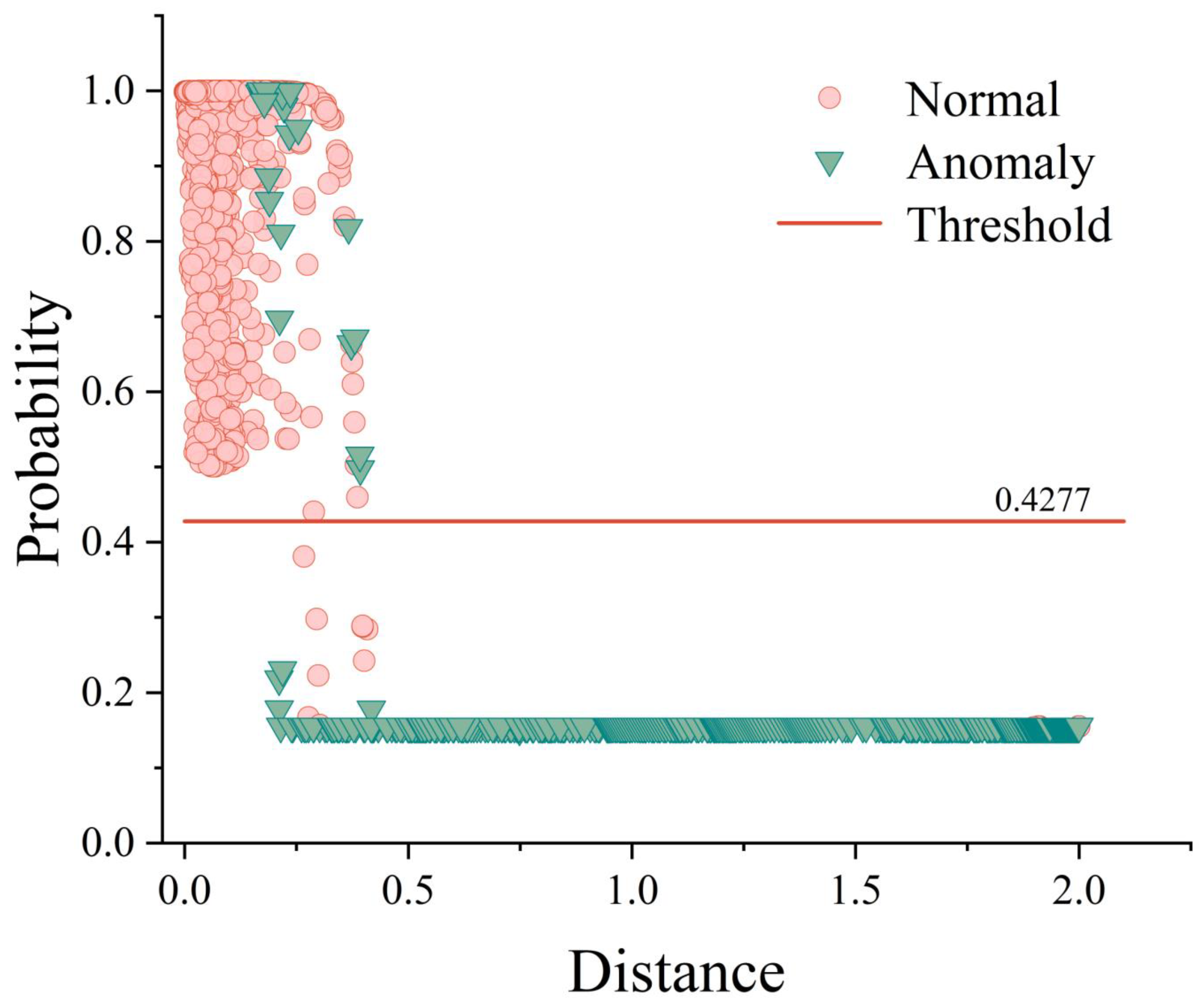
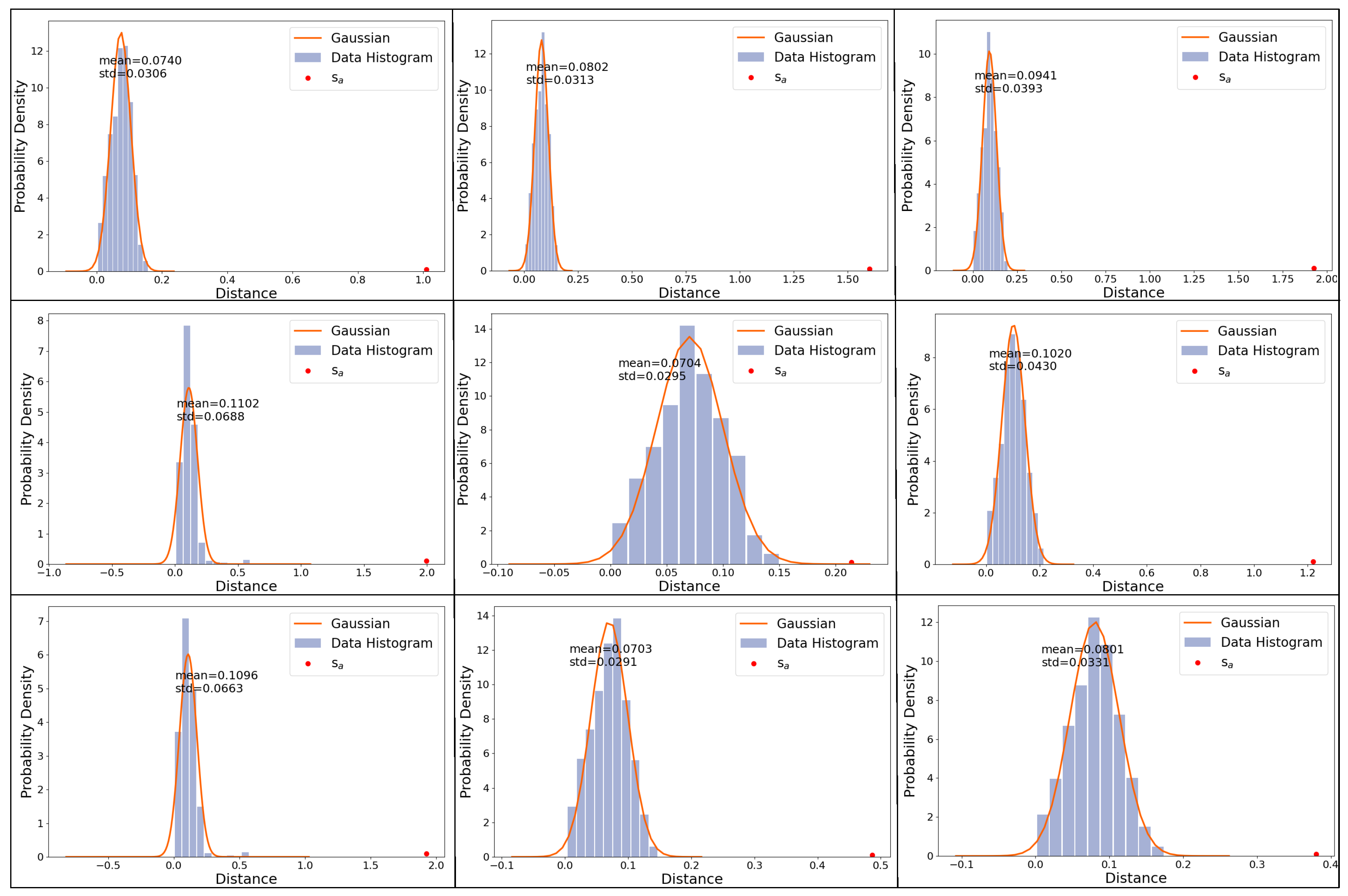
The reason why the performance of the Kernel SOM + Bayesian Posterior Inference model is always better than that of the Kernel SOM model is that the Kernel SOM + Bayesian Posterior Inference model builds a distance distribution probability model reflecting the data of each clustering cluster based on the Kernel SOM. The distance distribution probability model accurately analyzes the data distribution pattern under normal conditions, which creates a clearer boundary between normal and abnormal states. Furthermore, combined with posterior inference, the Kernel SOM + Bayesian Posterior Inference model probabilistically infers the likelihood of data anomalies. Differing from the Kernel SOM that solely relies on distance measurement, this method considers the intrinsic structure and distribution of data. This improves the model’s accuracy in anomaly detection. As shown in Figure 4, the Kernel SOM + Bayesian Posterior Inference model establishes a clear probabilistic boundary between normal and abnormal samples, effectively achieving the separation and identification of normal and abnormal samples.

5. Discussion

In this section, the superiority of the proposed method is demonstrated by comparing it with other state-of-the-art anomaly detection methods. The comparison emphasizes the proposed method’s better ability to identify abnormal samples, highlighting its outstanding anomaly detection capability. In addition, the explainability of the model’s decision-making process is thoroughly studied and explained in this section.

5.1. Method Superiority Verification

To verify the effectiveness and superiority of the proposed method, we compared the Kernel SOM + Bayesian Posterior Inference framework with advanced unsupervised anomaly detection algorithms for an RCP on the RCP monitoring data shown in Table 1. The compared algorithms included VAE + iForest [23] and CAAE-SA [24], as well as traditional anomaly detection methods such as iForest, AE, Local Outlier Factor (LOF) [30,31], One-Class SVM (OCSVM) [32], Denoising Autoencoder (DAE) [33], and Sparse Autoencoder (SAE) [34]. In the comparative experiments, all competing models requiring hyperparameter optimization were meticulously tuned. For deep unsupervised algorithms, including CAAE-SA, VAE + iForest, AE, DAE, and SAE, key parameters, such as learning rates, were primarily optimized through performance comparisons across different values within defined ranges to identify optimal learning rates. Similarly, for traditional machine learning methods, parameter optimization was conducted on the number of estimators in iForest, the neighborhood parameter in LOF, and the kernel parameters in OCSVM. This process involved systematically defining parameter ranges and evaluating model performance across different parameter values within these ranges to determine optimal algorithmic configurations.

The confusion matrices of various methods’ detection results based on RCP monitoring data are presented in Figure 5, with quantitative comparisons of corresponding performance metrics shown in

Table 5. Comparison results of different anomaly detection methods.

Method	Precision	Recall	F1-Score	Lag Time (h)
VAE + iForest	0.9626	0.9832	0.9728	10
CAAE-SA	0.9435	0.9598	0.9516	23
iForest	0.9916	0.9018	0.9446	31
AE	0.9508	0.7868	0.8610	14
LOF	0.9923	0.9781	0.9851	15
OCSVM	0.9947	0.9588	0.9764	11
DAE	0.9912	0.7471	0.8520	36
SAE	0.9850	0.8015	0.8838	36
Kernel SOM + Bayesian Posterior Inference	0.9938	0.9847	0.9893	8

.

Analyzing Figure 5 and Table 5 show that the proposed method correctly identified 1935 abnormal samples, which is higher than other models involved in the comparison. In terms of the comprehensive performance indicator F1-score, it also achieved the optimal value of 0.9893, outperforming other comparative models and demonstrating more excellent comprehensive performance. For lag time, Kernel SOM + Bayesian Posterior Inference exhibited an 8-h detection delay, outperforming all other models in alarm timeliness.

Overall, the Kernel SOM + Bayesian Posterior Inference model exhibited lower false positives and false negatives compared to other models, achieving high accuracy in anomaly detection. These results validate the superiority of the proposed algorithm in RCP anomaly detection.

In addition, the gear dataset from the University of Connecticut [35,36], which contains both lower differentiated and distinctly anomalous data relative to normal states, was used to assess the universality of the proposed method further. For this validation, we designated the “Missing”, “Cracked”, “Spalled”, and severe “Chipped” fault data in the gear dataset as anomalous classes. A sliding window approach with a window size of 1000 s and a step size of 500 s was applied to extract samples from both normal and abnormal data, which were subsequently used for model validation. The sampling results are presented in

Table 6. The information of the verification data for the gear dataset.

Accident Types	Number of Samples	Number of Training Samples	Number of Testing Samples
Normal	624	444	180
Anomaly	2496	0	2496

, while the validation results are shown in

Table 7. Validation results of the Kernel SOM + Bayesian Posterior Inference for the gear dataset.

Method	Precision	Recall	F1-Score
Kernel SOM + Bayesian Posterior Inference	0.9979	0.9471	0.9718

.

As shown in Table 7, the proposed method demonstrates superior detection performance on the gear dataset, achieving a comprehensive F1-score of 0.9718. This indicates low rates of false positives and false negatives, thereby validating the method’s robust generalization capability and its potential applicability in other industrial anomaly detection scenarios.

5.2. Model Interpretability

The proposed model has high interpretability and traceability. It enables a clear understanding of how anomaly detection decisions are made and what factors affect the outcomes. This improves operators’ comprehension of the decision-making process in anomaly detection. To illustrate this, we present a case study utilizing a sample from the verification dataset.

5.2.1. Decision Interpretability

To further analyze how the decision was specifically achieved, the $s_a$, an abnormal sample from the RCP monitoring data, was selected for further analysis. According to our anomaly detection framework, $s_a$ is classified as an anomaly because its best match with the typical normal state patterns represented by the clustering centroids falls below the threshold. To provide a detailed analysis of how this result was derived, we examined the posterior probabilities of $s_a$ matching each typical normal-state pattern, along with the prior knowledge required for posterior probability computation, as shown in

Table 8. Posterior probability calculation parameters and results for $s_a$.

Cluster	${\mathit{c}}_1$	${\mathit{c}}_2$	${\mathit{c}}_3$	${\mathit{c}}_4$	${\mathit{c}}_5$	${\mathit{c}}_6$	${\mathit{c}}_7$	${\mathit{c}}_8$	${\mathit{c}}_9$
Kernel distance	1.0102	1.6018	1.9271	1.9974	0.2141	1.2208	1.9261	0.4866	0.3803
Likelihood function	0.0001	0.0001	0.0001	0.0001	0.0001	0.0001	0.0001	0.0001	0.0001
Prior probability	0.1219	0.1202	0.1257	0.1006	0.1179	0.0990	0.1008	0.1288	0.0911
Posterior probability	0.1394	0.1135	0.0828	0.0741	0.1411	0.0937	0.0775	0.1552	0.1227

Bold black indicates normal clustered clusters with the highest degree of match to $s_a$.

.

As evidenced in Table 8, sample $s_a$’s maximum posterior probability across all clusters is 0.1552, which falls below the threshold of 0.4277 (illustrated in Figure 4), thus being classified as abnormal. This outcome originates from $s_a$’s extremely low likelihood values in all clusters, as governed by the posterior probability calculation formula. To investigate the root cause of these depressed likelihood values, we visualize the kernel distance probability distribution model. As illustrated in Figure 6, $s_a$’s kernel distances to all cluster centroids exceed the normal operational ranges defined by the model, forcing the likelihood values to the predefined minimum value, ultimately resulting in the posterior probability that falls below the threshold. This systematic analysis clarifies the model’s decision-making process, aiding operators in understanding how abnormal decisions are made.

These principles and mechanisms also explain why the performance of the Kernel SOM + Bayesian Posterior Inference model is superior to that of the traditional Kernel SOM. By constructing a kernel distance probability distribution model, the proposed method provides a more detailed and accurate description of the kernel distance distributions for each cluster centroid, thereby establishing a clearer demarcation between normal and anomalous patterns. Consequently, anomalous patterns are assigned significantly lower values during the likelihood function calculation. Moreover, in the posterior probability computation, unlike Kernel SOM, the boundary between normal and anomalous modes is determined based on statistical distributions and probability density rather than a simple distance threshold. This gives the detection decision process a stronger theoretical foundation and better stability, leading to superior overall performance.

5.2.2. Feature Impact Interpretability

Building on the interpretable decision outcomes, we further investigate feature-specific contributions to kernel distance calculations to identify features significantly influencing anomaly detection. According to the definition of the RBF kernel, the kernel distance calculation for Kernel SOM is given by Equation (15). Analysis of Equation (15) shows that when the kernel parameter $\sigma$ is fixed, the kernel distance is determined by the Euclidean distance $\parallel {\mathbf{s}}_a{-\mathbf{c}\parallel }_2$ between sample ${\mathbf{s}}_a$ and cluster centroid $\mathbf{c}$ in the original feature space. This direct dependency implies that deviations in Euclidean distance fundamentally drive kernel distance variations. Therefore, quantifying individual feature contributions to the Euclidean distance enables explicit interpretation of their impact on anomaly detection results through the relationship.

$$d_{kernel}({\mathbf{s}}_{\mathbf{a}},\mathbf{c})=e^{(-{\displaystyle \frac{\Vert {\mathbf{s}}_{\mathbf{a}}-{\mathbf{s}}_{\mathbf{a}}{\Vert }^2}{2{\sigma }^2}})}-2e^{(-{\displaystyle \frac{\Vert {\mathbf{s}}_{\mathbf{a}}{-\mathbf{c}\Vert }^2}{2{\sigma }^2}})}+e^{(-{\displaystyle \frac{{\Vert \mathbf{c}-\mathbf{c}\Vert }^2}{2{\sigma }^2}})}=2(1-e^{(-{\displaystyle \frac{\Vert {\mathbf{s}}_{\mathbf{a}}{-\mathbf{c}\Vert }^2}{2{\sigma }^2}})})$$

(15)

According to the principle of Euclidean distance calculation, we designed Equation (16) to quantify the contribution of each feature $f_k$ to the kernel distance, where $w\left(f_k\right)$ represents the contribution value of $f_k$, and ${\mathbf{s}}_{\mathbf{a}}\left(f_k\right)$ and $\mathbf{c}\left(f_k\right)$ denote the values of ${\mathbf{s}}_{\mathbf{a}}$ and centroid $\mathbf{c}$ in feature $f_k$, respectively.

$$w\left(f_k\right)={\displaystyle \frac{{[{\mathbf{s}}_{\mathbf{a}}\left(f_k\right)-\mathbf{c}\left(f_k\right)]}^2}{{\displaystyle \sum _{j=1}^{11}}{[{\mathbf{s}}_{\mathbf{a}}\left(f_j\right)-\mathbf{c}\left(f_j\right)]}^2}}$$

(16)

Based on the decision criteria, the cluster $c_8$, which exhibits the highest probabilistic matching degree with sample $s_a$ has been selected to analyze the contributions of various features to the kernel distance and to infer the factors that play a decisive role in anomaly detection. The feature contribution result for $s_a$ is shown in Figure 7. As seen in Figure 7, features $f_1$ (Max), $f_2$ (Min), $f_4$ (Mean), $f_5$ (Slope), and $f_6$ (Root Mean Square) predominantly govern the kernel distance calculation for $s_a$, critically influencing its anomaly determination. These features primarily reflect amplitude variation, central tendency shift, and fluctuation intensity changes. A comparison of monitoring signal values between normal and anomalous patterns in Figure 2 reveals significant pressure monitoring value reductions in anomalous states compared to normal states. The pronounced deviations in both amplitude and central tendency ultimately lead the model to classify the sample as anomalous. This analytical approach precisely localizes the root causes of deviations between normal and anomalous states, providing actionable evidence for confirming anomaly occurrences. This feature impact analysis pinpoints the root causes of deviations between abnormal and normal states, providing actionable evidence for confirming anomaly occurrences.

To investigate whether the proposed method can accurately identify features critical to decision-making across different datasets, the sample $s_m$ from the ‘Missing’ fault type of the gear dataset, which exhibits lower deviations from normal conditions, was selected for analysis. The result of the analysis is presented in Figure 8.

Figure 8 reveals that features $f_1$ (Max), $f_2$ (Min), $f_3$ (Range), $f_6$ (RMS), and $f_7$ (Skewness) play a dominant role in the anomaly classification of the sample $s_m$. These features primarily capture discrepancies in amplitude and fluctuation intensity between the ’Missing’ fault state and normal operational conditions. Notably, this aligns well with the physical understanding that vibration signals from gears with missing teeth exhibit distinct amplitude variations and fluctuation patterns compared to normal signals. This analysis underscores the methodology’s validity and accuracy, demonstrating its ability to leverage feature-driven decision logic for reliable anomaly detection across diverse datasets.

It is important to note that in analyzing the impact of features on the decision outcome, we assess their contribution based on the kernel distance calculation method used in this study, specifically the RBF kernel. Moreover, this analytical approach remains valid even if the distance calculation method is replaced with an alternative approach.

6. Conclusions

To address the insufficient interpretability of existing anomaly detection methods for RCP equipment, this study proposes an unsupervised anomaly detection algorithm based on Kernel SOM and Bayesian Posterior Inference. This framework provides an interpretable solution for RCP anomaly identification. The method establishes a precise boundary between normal and abnormal states by constructing a kernel distance probability distribution model for clustering results, providing both a reliable data distribution analysis tool and an interpretable model to enhance anomaly discernibility. Furthermore, by integrating the kernel distance distribution model with Bayesian Posterior Inference, the framework enables probabilistic anomaly assessment and traceable decision-making processes, significantly improving detection performance and interpretability. The verification results demonstrate that the proposed method outperforms other existing advanced and traditional algorithms in detection accuracy. Additionally, the method systematically explains the rationale behind anomaly judgments and identifies critical features influencing detection outcomes, aiding users in pinpointing the root causes of anomalies and distinguishing abnormal from normal patterns.

The proposed method can be applied not only to anomaly detection in RCPs but also to equipment anomaly detection in other engineering fields. Its modules are relatively independent, allowing components such as the clustering module to be adjusted or replaced based on the specific application scenario, which demonstrates its broad potential for use. However, current verification is limited to univariate data due to data acquisition constraints. Future work will extend the method to multivariate data to further enhance anomaly detection rates.

References

1. Ran, T.; Xiao, R.; Liu, W. Investigation of the flow characteristics in a main nuclear power plant pump with eccentric impeller. Nucl. Eng. Des. 2018, 327, 70–81. [Google Scholar]
2. Qian, G.; Liu, J. Development of deep reinforcement learning-based fault diagnosis method for rotating machinery in nuclear power plants. Prog. Nucl. Energy 2022, 152, 104401. [Google Scholar] [CrossRef]
3. Lee, G.; Lee, S.J.; Lee, C. A convolutional neural network model for abnormality diagnosis in a nuclear power plant. Appl. Soft Comput. 2021, 99, 106874. [Google Scholar] [CrossRef]
4. Wang, X.; Lu, Y.; Zhu, R.; Fu, Q.; Chen, Y.; Zhong, W. Experimental study on transient characteristics of reactor coolant pump under rotor seizure accident. Ann. Nucl. Energy 2020, 136, 107039. [Google Scholar] [CrossRef]
5. Ayodeji, A.; Liu, Y.K.; Xia, H. Knowledge base operator support system for nuclear power plant fault diagnosis. Prog. Nucl. Energy 2018, 105, 42–50. [Google Scholar] [CrossRef]
6. Biet, M. Rotor faults diagnosis using feature selection and nearest neighbors rule: Application to a turbogenerator. IEEE Trans. Ind. Electron. 2012, 60, 4063–4073. [Google Scholar] [CrossRef]
7. Ayodeji, A.; Liu, Y.K. Support vector ensemble for incipient fault diagnosis in nuclear plant components. Nucl. Eng. Technol. 2018, 50, 1306–1313. [Google Scholar] [CrossRef]
8. Wang, H.; Peng, M.J.; Hines, J.W.; Zheng, G.y.; Liu, Y.; Upadhyaya, B.R. A hybrid fault diagnosis methodology with support vector machine and improved particle swarm optimization for nuclear power plants. ISA Trans. 2019, 95, 358–371. [Google Scholar] [CrossRef]
9. Du, J.; Liu, P.; Vong, C.M.; Chen, C.; Wang, T.; Chen, C.P. Class-incremental learning method with fast update and high retainability based on broad learning system. IEEE Trans. Neural Netw. Learn. Syst. 2023, 35, 11332–11345. [Google Scholar] [CrossRef]
10. Aizpurua, J.I.; McArthur, S.D.; Stewart, B.G.; Lambert, B.; Cross, J.G.; Catterson, V.M. Adaptive power transformer lifetime predictions through machine learning and uncertainty modeling in nuclear power plants. IEEE Trans. Ind. Electron. 2018, 66, 4726–4737. [Google Scholar] [CrossRef]
11. Dong, F.; Chen, S.; Demachi, K.; Yoshikawa, M.; Seki, A.; Takaya, S. Attention-based time series analysis for data-driven anomaly detection in nuclear power plants. Nucl. Eng. Des. 2023, 404, 112161. [Google Scholar] [CrossRef]
12. Yao, Y.; Wang, J.; Long, P.; Xie, M.; Wang, J. Small-batch-size convolutional neural network based fault diagnosis system for nuclear energy production safety with big-data environment. Int. J. Energy Res. 2020, 44, 5841–5855. [Google Scholar] [CrossRef]
13. Wang, C.; Liu, J. Reactor Coolant Pump Leakage Estimation of PWR Based on Broad Learning System. J. Phys. Conf. Ser. 2021, 1939, 012102. [Google Scholar] [CrossRef]
14. Yang, T.; Ma, J.; Yuan, J.; Wang, S. Reactor Coolant System Fault Diagnosis Method Using Symmetrized Dot Pattern Images and DSCNN. In Proceedings of the 2023 CAA Symposium on Fault Detection, Supervision and Safety for Technical Processes (SAFEPROCESS), Yibin, China, 22–24 September 2023; pp. 1–6. [Google Scholar]
15. Zhang, J.; Liang, J.; Liu, J. Fault diagnosis in reactor coolant pump with an automatic CNN-based mixed model. Prog. Nucl. Energy 2024, 175, 105294. [Google Scholar] [CrossRef]
16. Chen, Y.; Ashizawa, N.; Yeo, C.K.; Yanai, N.; Yean, S. Multi-scale self-organizing map assisted deep autoencoding Gaussian mixture model for unsupervised intrusion detection. Knowl.-Based Syst. 2021, 224, 107086. [Google Scholar] [CrossRef]
17. Abhaya, A.; Patra, B.K. An efficient method for autoencoder based outlier detection. Expert Syst. Appl. 2023, 213, 118904. [Google Scholar] [CrossRef]
18. Zhang, C.; Geng, Y.; Han, Z.; Liu, Y.; Fu, H.; Hu, Q. Autoencoder in autoencoder networks. IEEE Trans. Neural Netw. Learn. Syst. 2022, 35, 2263–2275. [Google Scholar] [CrossRef]
19. Toshpulatov, M.; Zincir-Heywood, N. Anomaly detection on smart meters using hierarchical self-organizing maps. In Proceedings of the 2021 IEEE Canadian Conference on Electrical and Computer Engineering (CCECE), Virtual, 12–17 September 2021; pp. 1–6. [Google Scholar]
20. Concetti, L.; Mazzuto, G.; Ciarapica, F.E.; Bevilacqua, M. An Unsupervised Anomaly Detection Based on Self-Organizing Map for the Oil and Gas Sector. Appl. Sci. 2023, 13, 3725. [Google Scholar] [CrossRef]
21. Vanem, E.; Brandsæter, A. Unsupervised anomaly detection based on clustering methods and sensor data on a marine diesel engine. J. Mar. Eng. Technol. 2021, 20, 217–234. [Google Scholar] [CrossRef]
22. Cancemi, S.; Frano, R.L.; Santus, C.; Inoue, T. Unsupervised anomaly detection in pressurized water reactor digital twins using autoencoder neural networks. Nucl. Eng. Des. 2023, 413, 112502. [Google Scholar] [CrossRef]
23. Li, X.; Huang, T.; Cheng, K.; Qiu, Z.; Sichao, T. Research on anomaly detection method of nuclear power plant operation state based on unsupervised deep generative model. Ann. Nucl. Energy 2022, 167, 108785. [Google Scholar] [CrossRef]
24. Sun, X.; Guo, S.; Liu, S.; Guo, J.; Du, B. Unsupervised anomaly detection of nuclear power plants under noise background based on convolutional adversarial autoencoder combining self-attention mechanism. Nucl. Eng. Des. 2024, 428, 113493. [Google Scholar] [CrossRef]
25. Lau, K.W.; Yin, H.; Hubbard, S. Kernel self-organising maps for classification. Neurocomputing 2006, 69, 2033–2040. [Google Scholar] [CrossRef]
26. Ngu, J.C.Y.; Yeo, W.S.; Thien, T.F.; Nandong, J. A comprehensive overview of the applications of kernel functions and data-driven models in regression and classification tasks in the context of software sensors. Appl. Soft Comput. 2024, 164, 111975. [Google Scholar] [CrossRef]
27. Guo, B.; Song, L.; Zheng, T.; Liang, H.; Wang, H. A comparative evaluation of SOM-based anomaly detection methods for multivariate data. In Proceedings of the 2019 Prognostics and System Health Management Conference (PHM-Qingdao), Qingdao, China, 25–27 October 2019; pp. 1–6. [Google Scholar]
28. Li, Z.; Zhu, Y.; Van Leeuwen, M. A survey on explainable anomaly detection. ACM Trans. Knowl. Discov. Data 2023, 18, 1–54. [Google Scholar] [CrossRef]
29. Pukelsheim, F. The three sigma rule. Am. Stat. 1994, 48, 88–91. [Google Scholar] [CrossRef]
30. Nowak Brzezińska, A.; Horyń, C. Outliers in rules-the comparision of LOF, COF and KMEANS algorithms. Procedia Comput. Sci. 2020, 176, 1420–1429. [Google Scholar] [CrossRef]
31. Chugh, B.; Malik, N.; Gupta, D.; Alkahtani, B.S. A probabilistic approach driven credit card anomaly detection with CBLOF and isolation forest models. Alex. Eng. J. 2025, 114, 231–242. [Google Scholar] [CrossRef]
32. Binbusayyis, A.; Vaiyapuri, T. Unsupervised deep learning approach for network intrusion detection combining convolutional autoencoder and one-class SVM. Appl. Intell. 2021, 51, 7094–7108. [Google Scholar] [CrossRef]
33. Xu, F.; Yang, F.; Fei, Z.; Huang, Z.; Tsui, K.L. Life prediction of lithium-ion batteries based on stacked denoising autoencoders. Reliab. Eng. Syst. Saf. 2021, 208, 107396. [Google Scholar] [CrossRef]
34. Qiu, Y.; Zhou, W.; Yu, N.; Du, P. Denoising sparse autoencoder-based ictal EEG classification. IEEE Trans. Neural Syst. Rehabil. Eng. 2018, 26, 1717–1726. [Google Scholar] [CrossRef] [PubMed]
35. Li, W.; Zhong, X.; Shao, H.; Cai, B.; Yang, X. Multi-mode data augmentation and fault diagnosis of rotating machinery using modified ACGAN designed with new framework. Adv. Eng. Inform. 2022, 52, 101552. [Google Scholar] [CrossRef]
36. Zhu, X.; Yang, D.; Pan, H.; Karimi, H.R.; Ozevin, D.; Cetin, A.E. A novel asymmetrical autoencoder with a sparsifying discrete cosine stockwell transform layer for gearbox sensor data compression. Eng. Appl. Artif. Intell. 2024, 127, 107322. [Google Scholar] [CrossRef]
Figure 1. The overall framework of the anomaly detection method based on Kernel SOM + Bayesian Posterior Inference.
Energies 18 02887 g001
Figure 2. Pressure monitoring data of the mechanical seal of the RCP.
Energies 18 02887 g002
Figure 3. Feature distributions under different states.
Energies 18 02887 g003
Figure 4. Prediction results of the posterior probability by Kernel SOM + Bayesian Posterior Inference.
Energies 18 02887 g004
Figure 5. Confusion matrices of detection results for different anomaly detection methods.
Energies 18 02887 g005
Figure 6. Visualization of the Gaussian model for kernel distance probability distribution for RCP monitoring data.
Energies 18 02887 g006
Figure 7. Contributions of different features to kernel distances of the sample s a .
Energies 18 02887 g007
Figure 8. Contributions of different features to kernel distances of the sample s m .
Energies 18 02887 g008