Small-Disturbance Stability Analysis of Doubly Fed Variable-Speed Pumped Storage Units

Abstract

The variable-speed operation mode of pumped storage units improves the regulation performance and endows the units with characteristics such as isolation from the power grid, thereby affecting the system stability. This study establishes a detailed mathematical model for the connection of doubly fed induction generator-based variable-speed pumped storage (DFIG-VSPS) to a single-machine infinite bus system under power generation conditions in the synchronous rotation direct-quadrature-zero coordinate system. The introduction of the eigenvalue method to analyze the small-disturbance stability of doubly fed variable-speed pumped storage units and the use of participation factors to calculate the degree of influence of each state variable on the small-disturbance stability of the units are innovations of this study. The participation factor enhances flexibility, continuity, and efficiency in doubly fed variable-speed pumped storage by optimizing dynamic power paths and enabling multi-objective control coordination. While eigenvalue analysis is not new, this study is the first to apply it with participation factors to DFIG-VSPS, addressing gaps in prior simplified models. Furthermore, based on the changes in the characteristic root trajectories, the influence of changes in the speed control system parameters and converter controller parameters on the system stability was determined. Finally, the conclusions obtained were verified through simulation. The results indicate that increasing the time constant of water flow inertia poses a risk of system instability, and the increase in proportional parameters and decrease in integral parameters of the power outer loop controller significantly affect the system stability.

1. Introduction

With the gradual increase in the penetration rate of renewable energy sources, such as wind power and photovoltaic solar power, the problems of power fluctuation and frequency regulation are becoming increasingly prominent. The operation of modern power grids requires faster responses, larger regulation capacities, and more flexible operational methods. The variable-speed operation of units in pumped storage power plants can provide additional flexibility to the power system [1,2,3]. Using variable-speed pumped storage (VSPS) can improve the dynamic performance of a power system, quickly stabilize the system frequency, promote new energy consumption, and improve energy use efficiency, thereby providing vital support for the safe and stable operation of the power grid and the construction of a new type of power system [4].

Doubly fed induction generator-based VSPS (DFIG-VSPS) (see Abbreviations) has been widely studied and applied in high-capacity applications owing to its low requirements for converter capacity and fast power regulation performance [5,6]. Although the DFIG improves the performance of the unit, it introduces new characteristics into the regulating system of the pump turbine. The excitation system and control strategy of the unit becomes complex, presenting a nonlinear system with a strong coupling of water, machinery, electricity, and control. The use of inverters results in isolation between the unit and power grid, decoupling the unit speed from the grid frequency, and the unit no longer provides inertial reserves for the power grid. These new characteristics inevitably have new impacts on the stability of both the unit and power grid. Therefore, it is necessary to study the small interference stability of the DFIG-VSPS.

Small-signal modeling forms the basis of small-disturbance stability analysis. To simulate the dynamic characteristics of the DFIG-VSPS unit, Lung et al. [7] improved the mathematical model of the doubly fed motor and established an overall mathematical model of the DFIG-VSPS by combining it with the ideal model of the pump turbine. Gao et al. [8] established a simplified electromechanical transient model of DFIG-VSPS by making reasonable assumptions and neglecting the dynamic processes of the grid side control, rotor-side reactive power control, and converter switching tubes of the DFIG. However, their model is only applicable to the study of pump turbine regulation systems. Zhao et al. [9] studied the multi-scale oscillation characteristics and stability of low head grid connected pumped storage units under primary frequency regulation conditions. During the operation of pumped storage units, the lower the head, the poorer the system stability. Li [10] proposed a new excitation control method when establishing the electromechanical transient model of VSPS in which the rotor flux dynamics was considered. However, some of the parameters in the model have poor response fitting and are unsuitable for small signal stability analysis; it was unable to perform small signal stability analysis. Zhang [11] adopted an improved inertia control scheme for doubly fed wind turbines to improve the stability of the motor rotor and verified the conclusion by integrating it into a four-machine two-zone model. Gebru et al. [12] provided a comparative analysis of the inverter of doubly fed fans under steady-state and symmetrical fault conditions. Xu et al. [13] proposed a state space model for doubly fed wind turbines connected to weak AC power grids, which is suitable for the time-scale reduction of electromechanical transients. The latter three studies [11,12,13] have conducted corresponding research on doubly fed wind turbines, and their application in the analysis of the prime mover and control mode of VSPS encompasses certain differences. Han et al. [14] applied eigenvalue analysis to the stability study of VSPS; however, the use of a simplified model with a converter affected the accuracy of system stability analysis. Wang et al. [15] established a broadband impedance model for the joint operation system of doubly fed pumped storage units and direct drive wind turbines. However, their research focus was on the coupling problem between the doubly fed wind turbines and the DFIG-VSPS control system parameters and frequency accuracy, without a separate analysis of the control parameters of the DFIG-VSPS. In summary, while several studies have been conducted on DFIG-VSPS and DFIG, the existing literature lacks accurate small-signal modeling or small-disturbance stability analysis on the units.

In this study, a mathematical model of DFIG-VSPS is established. To ensure the reliability of the conclusions, the pump turbine, DFIG, and controller of VSPS under power generation conditions are considered, and a complete small-signal model is constructed. Subsequently, the eigenvalue method is used to perform small-signal stability analysis on the system, and the interactions between various state variables in the system are explored based on the participation factors. Based on the root trajectory curve of the system, the influence of changes in pump turbine parameters, DFIG parameters, and several controller parameters on system stability were determined and finally verified through time–domain simulation.

2. Mathematical Model of DFIG-VSPS

2.1. DFIG Model

While the dynamic model of a doubly fed induction generator (DFIG) in the dq0 synchronous rotating frame exhibits rapidly decaying stator-side transients during small signal stability analysis, the time scale of the studied stability phenomena (e.g., electromechanical oscillations, typically in the range of 0.1–2 Hz) is significantly longer than the stator flux transient dynamics (with time constants on the order of 10–50 ms) [16]. This temporal separation ensures that neglecting stator flux transients does not materially affect the accuracy of the stability analysis, as their influence diminishes well before the dominant modes of interest manifest. Furthermore, this simplification reduces computational complexity without compromising the validity of the results for the studied time-scale phenomena. The simplified DFIG diagram is shown in Figure 1.

We consider the transient electromotive force $E_{\mathrm{d}}^{\prime }$, $E_{\mathrm{q}}^{\prime }$, and transient reactance $X^{\prime }$ of nodes within the generator, which includes

$${\displaystyle \frac{\mathrm{d}{\phi }_{\mathrm{ds}}}{\mathrm{d}t}}=0,{\displaystyle \frac{\mathrm{d}{\phi }_{\mathrm{qs}}}{\mathrm{d}t}}=0$$

(1)

Subsequently, the stator voltage equation can be transformed into

$$\left\{\begin{array}{l}{u}_{\mathrm{ds}}=R_{\mathrm{s}}{i}_{\mathrm{ds}}-X^{\prime }{i}_{\mathrm{qs}}+E_{\mathrm{d}}^{\prime }\\ u_{\mathrm{qs}}=R_{\mathrm{s}}{i}_{\mathrm{qs}}+X^{\prime }{i}_{\mathrm{ds}}+E_{\mathrm{q}}^{\prime }\end{array}\right.$$

(2)

wherein

$$\left\{\begin{array}{l}{E}_{\mathrm{d}}^{\prime }=-{\displaystyle \frac{{\omega }_{\mathrm{s}}{L}_{\mathrm{m}}}{L_{\mathrm{r}}}}{\phi }_{\mathrm{qr}}\\ E_{\mathrm{q}}^{\prime }={\displaystyle \frac{{\omega }_{\mathrm{s}}{L}_{\mathrm{m}}}{L_{\mathrm{r}}}}{\phi }_{\mathrm{dr}}\\ X^{\prime }={\displaystyle \frac{{\omega }_{\mathrm{s}}}{L_{\mathrm{r}}}}(L_{\mathrm{s}}{L}_{\mathrm{r}}-L_{\mathrm{m}}^2)\end{array}\right.$$

(3)

where L_s, L_r, and L_m are the stator inductance, rotor inductance, and mutual inductance of the DFIG. Introducing Equation (3) into the flux linkage equation of DFIG yields [8]

$$\left\{\begin{array}{l}{\phi }_{\mathrm{ds}}={\displaystyle \frac{L_{\mathrm{s}}}{L_{\mathrm{m}}}}{\phi }_{\mathrm{dr}}-{\displaystyle \frac{L_{\mathrm{s}}{L}_{\mathrm{r}}-L_{\mathrm{m}}^2}{L_{\mathrm{m}}}}{i}_{\mathrm{dr}}\\ \hspace{1em} ={\displaystyle \frac{L_{\mathrm{s}}{L}_{\mathrm{r}}}{{\omega }_{\mathrm{s}}{L}_{\mathrm{m}}^2}}{E}_{\mathrm{q}}^{\prime }-{\displaystyle \frac{L_{\mathrm{r}}{X}^{\prime }}{{\omega }_{\mathrm{s}}{L}_{\mathrm{m}}}}{i}_{\mathrm{dr}}\\ {\phi }_{\mathrm{qs}}={\displaystyle \frac{L_{\mathrm{s}}}{L_{\mathrm{m}}}}{\phi }_{\mathrm{qr}}-{\displaystyle \frac{L_{\mathrm{s}}{L}_{\mathrm{r}}-L_{\mathrm{m}}^2}{L_{\mathrm{m}}}}{i}_{\mathrm{qr}}\\ \hspace{1em} =-{\displaystyle \frac{L_{\mathrm{s}}{L}_{\mathrm{r}}}{{\omega }_{\mathrm{s}}{L}_{\mathrm{m}}^2}}{E}_{\mathrm{d}}^{\prime }-{\displaystyle \frac{L_{\mathrm{r}}{X}^{\prime }}{{\omega }_{\mathrm{s}}{L}_{\mathrm{m}}}}{i}_{\mathrm{qr}}\\ i_{\mathrm{ds}}={\displaystyle \frac{{\phi }_{\mathrm{dr}}}{L_{\mathrm{m}}}}-{\displaystyle \frac{L_{\mathrm{r}}}{L_{\mathrm{m}}}}{i}_{\mathrm{dr}}={\displaystyle \frac{L_{\mathrm{r}}}{{\omega }_{\mathrm{s}}{L}_{\mathrm{m}}^2}}{E}_{\mathrm{q}}^{\prime }-{\displaystyle \frac{L_{\mathrm{r}}}{L_{\mathrm{m}}}}{i}_{\mathrm{dr}}\\ i_{\mathrm{qs}}={\displaystyle \frac{{\phi }_{\mathrm{qr}}}{L_{\mathrm{m}}}}-{\displaystyle \frac{L_{\mathrm{r}}}{L_{\mathrm{m}}}}{i}_{\mathrm{dr}}=-{\displaystyle \frac{L_{\mathrm{r}}}{{\omega }_{\mathrm{s}}{L}_{\mathrm{m}}^2}}{E}_{\mathrm{d}}^{\prime }-{\displaystyle \frac{L_{\mathrm{r}}}{L_{\mathrm{m}}}}{i}_{\mathrm{qr}}\end{array}\right.$$

(4)

Introducing Equation (4) into the stator rotor voltage equation of DFIG yields

$$\left\{\begin{array}{l}{\displaystyle \frac{\mathrm{d}{E}_{\mathrm{d}}^{\prime }}{\mathrm{d}t}}=-{\displaystyle \frac{{\omega }_{\mathrm{s}}{L}_{\mathrm{m}}}{L_{\mathrm{r}}}}{u}_{\mathrm{qr}}+{\displaystyle \frac{{\omega }_{\mathrm{s}}{L}_{\mathrm{m}}}{L_{\mathrm{r}}}}{R}_{\mathrm{r}}{i}_{\mathrm{qr}}+\left({\omega }_{\mathrm{s}}-{\omega }_{\mathrm{r}}\right)E_{\mathrm{q}}^{\prime }\\ {\displaystyle \frac{\mathrm{d}{E}_{\mathrm{q}}^{\prime }}{\mathrm{d}t}}={\displaystyle \frac{{\omega }_{\mathrm{s}}{L}_{\mathrm{m}}}{L_{\mathrm{r}}}}{u}_{\mathrm{dr}}-{\displaystyle \frac{{\omega }_{\mathrm{s}}{L}_{\mathrm{m}}}{L_{\mathrm{r}}}}{R}_{\mathrm{r}}{i}_{\mathrm{dr}}-\left({\omega }_{\mathrm{s}}-{\omega }_{\mathrm{r}}\right)E_{\mathrm{d}}^{\prime }\\ {\displaystyle \frac{\mathrm{d}{i}_{\mathrm{dr}}}{\mathrm{d}t}}={\displaystyle \frac{{\omega }_{\mathrm{s}}{L}_{\mathrm{s}}}{X^{\prime }{L}_{\mathrm{r}}}}{u}_{\mathrm{dr}}-{\displaystyle \frac{{\omega }_{\mathrm{s}}{L}_{\mathrm{m}}}{X^{\prime }{L}_{\mathrm{r}}}}{u}_{\mathrm{ds}}-{\displaystyle \frac{{\omega }_{\mathrm{s}}}{X^{\prime }}}\left({\displaystyle \frac{L_{\mathrm{s}}}{L_{\mathrm{r}}}}{R}_{\mathrm{r}}+R_{\mathrm{s}}\right)i_{\mathrm{dr}}\\ \hspace{1em}\hspace{1em}+{\omega }_{\mathrm{s}}{i}_{\mathrm{qr}}+{\displaystyle \frac{L_{\mathrm{r}}}{X^{\prime }{L}_{\mathrm{m}}}}{\omega }_{\mathrm{r}}{E}_{\mathrm{d}}^{\prime }+{\displaystyle \frac{R_{\mathrm{s}}}{X^{\prime }{L}_{\mathrm{m}}}}{E}_{\mathrm{q}}^{\prime }\\ {\displaystyle \frac{\mathrm{d}{i}_{\mathrm{qr}}}{\mathrm{d}t}}={\displaystyle \frac{{\omega }_{\mathrm{s}}{L}_{\mathrm{s}}}{X^{\prime }{L}_{\mathrm{r}}}}{u}_{\mathrm{qr}}-{\displaystyle \frac{{\omega }_{\mathrm{s}}{L}_{\mathrm{m}}}{X^{\prime }{L}_{\mathrm{r}}}}{u}_{\mathrm{qs}}-{\displaystyle \frac{{\omega }_{\mathrm{s}}}{X^{\prime }}}\left({\displaystyle \frac{L_{\mathrm{s}}}{L_{\mathrm{r}}}}{R}_{\mathrm{r}}+R_{\mathrm{s}}\right)i_{\mathrm{qr}}\\ \hspace{1em}\hspace{1em}-{\omega }_{\mathrm{s}}{i}_{\mathrm{dr}}+{\displaystyle \frac{L_{\mathrm{r}}}{X^{\prime }{L}_{\mathrm{m}}}}{\omega }_{\mathrm{r}}{E}_{\mathrm{q}}^{\prime }-{\displaystyle \frac{R_{\mathrm{s}}}{X^{\prime }{L}_{\mathrm{m}}}}{E}_{\mathrm{d}}^{\prime }\end{array}\right.$$

(5)

Equation (5) constitutes a fourth-order transient model of DFIG using rotor current and rotor flux as state variables, which can accurately reflect the transient process of DFIG and facilitate subsequent small-signal stability analysis.

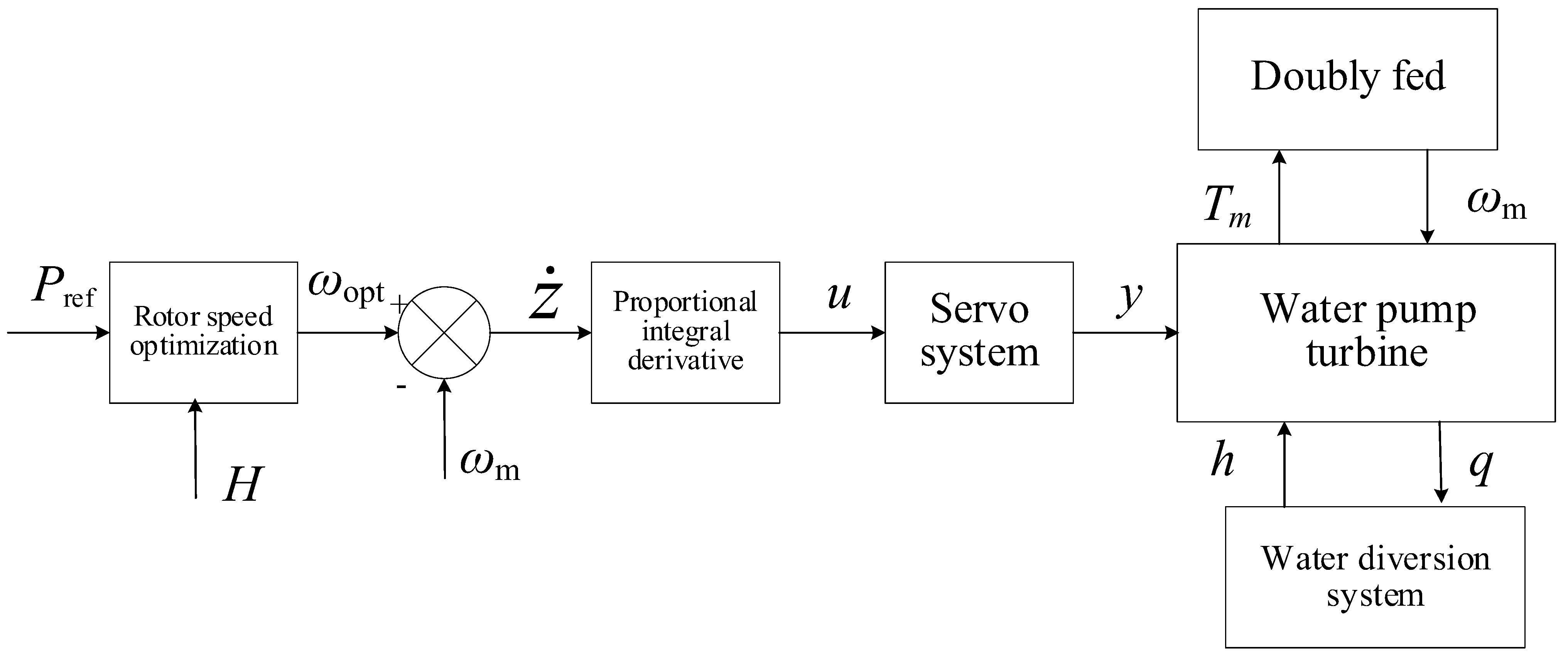
2.2. Pump Turbine and Speed Control System Model

The speed control system of a pump turbine primarily comprises a speed optimization system, governor, servo system, pump turbine and diversion system, and DFIG. The control structure is illustrated in Figure 2.

When studying the small-disturbance stability problem under a generating mode, the essence is that the unit, while operating stably, is subjected to a small disturbance, causing its operating condition to fluctuate slightly around the initial state without undergoing a fundamental change. Therefore, a linearized model described by six coefficients is adopted. Under a generating mode, the pump turbine unit can be treated as a conventional hydraulic turbine. The relationships between torque and flow versus head, speed, and guide vane opening can be described by Equation (6):

$$\left\{\begin{array}{l}{M}_{\mathrm{t}}=M_{\mathrm{t}}\left(H,n,\alpha \right)\\ Q=Q\left(H,n,\alpha \right)\end{array}\right.$$

(6)

where M_t is unit torque, Q is flow rate, H is working head, n is rotational speed, and α is guide vane opening.

For small signal stability analysis, linearization is performed around the steady-state operating point. Specifically, Equation (6) is expanded using a Taylor series, and higher-order terms (second order and above) are neglected, yielding:

$$\left\{\begin{array}{l}\Delta M_{\mathrm{t}}={\displaystyle \frac{\partial M_{\mathrm{t}}}{\partial \alpha }}\Delta \alpha +{\displaystyle \frac{\partial M_{\mathrm{t}}}{\partial n}}\Delta n+{\displaystyle \frac{\partial M_{\mathrm{t}}}{\partial H}}\Delta H\\ \Delta Q={\displaystyle \frac{\partial Q}{\partial \alpha }}\Delta \alpha +{\displaystyle \frac{\partial Q}{\partial n}}\Delta n+{\displaystyle \frac{\partial Q}{\partial H}}\Delta H\end{array}\right.$$

(7)

Expressed in per-unit (relative) values:

$$\left\{\begin{array}{l}{\displaystyle \frac{\Delta M_{\mathrm{t}}}{M_{\mathrm{r}}}}={\displaystyle \frac{\partial \frac{M_{\mathrm{t}}}{M_{\mathrm{r}}}}{\partial \frac{\alpha }{{\alpha }_{\max }}}}{\displaystyle \frac{\Delta \alpha }{{\alpha }_{\max }}}+{\displaystyle \frac{\partial \frac{M_{\mathrm{t}}}{M_{\mathrm{r}}}}{\partial \frac{n}{n_{\mathrm{r}}}}}{\displaystyle \frac{\Delta n}{n_{\mathrm{r}}}}+{\displaystyle \frac{\partial \frac{M_{\mathrm{t}}}{M_{\mathrm{r}}}}{\partial \frac{H}{H_{\mathrm{r}}}}}{\displaystyle \frac{\Delta H}{H_{\mathrm{r}}}}\\ {\displaystyle \frac{\Delta Q}{Q_{\mathrm{r}}}}={\displaystyle \frac{\partial \frac{Q}{Q_{\mathrm{r}}}}{\partial \frac{\alpha }{{\alpha }_{\max }}}}{\displaystyle \frac{\Delta \alpha }{{\alpha }_{\max }}}+{\displaystyle \frac{\partial \frac{Q}{Q_{\mathrm{r}}}}{\partial \frac{n}{n_{\mathrm{r}}}}}{\displaystyle \frac{\Delta n}{n_{\mathrm{r}}}}+{\displaystyle \frac{\partial \frac{Q}{Q_{\mathrm{r}}}}{\partial \frac{H}{H_{\mathrm{r}}}}}{\displaystyle \frac{\Delta H}{H_{\mathrm{r}}}}\end{array}\right.$$

(8)

The relative deviation of guide vane opening ${\displaystyle \frac{\Delta a}{a_{\max }}}$ exhibits a linear relationship with servomotor stroke ${\displaystyle \frac{\Delta Y}{Y_{\max }}}$, allowing for their interchangeable use in the analysis. Let:

$$\begin{array}{c}{\displaystyle \frac{\Delta M_{\mathrm{t}}}{M_{\mathrm{r}}}}=m_{\mathrm{t}}, {\displaystyle \frac{\Delta Q}{Q_{\mathrm{r}}}}=q, {\displaystyle \frac{\Delta a}{a_{\max }}}=y={\displaystyle \frac{\Delta Y}{Y_{\max }}}, {\displaystyle \frac{\Delta n}{n_{\mathrm{r}}}}=x, {\displaystyle \frac{\Delta H}{H_{\mathrm{r}}}}=h\\ e_{\mathrm{y}}={\displaystyle \frac{\partial \frac{M_{\mathrm{t}}}{M_{\mathrm{r}}}}{\partial \frac{\alpha }{{\alpha }_{\max }}}}, e_{\mathrm{x}}={\displaystyle \frac{\partial \frac{M_{\mathrm{t}}}{M_{\mathrm{r}}}}{\partial \frac{n}{n_{\mathrm{r}}}}}, e_{\mathrm{h}}={\displaystyle \frac{\partial \frac{M_{\mathrm{t}}}{M_{\mathrm{r}}}}{\partial \frac{H}{H_{\mathrm{r}}}}}\\ e_{\mathrm{qy}}={\displaystyle \frac{\partial \frac{Q}{Q_{\mathrm{r}}}}{\partial \frac{\alpha }{{\alpha }_{\max }}}},e_{\mathrm{qx}}={\displaystyle \frac{\partial \frac{Q}{Q_{\mathrm{r}}}}{\partial \frac{n}{n_{\mathrm{r}}}}},e_{\mathrm{qh}}={\displaystyle \frac{\partial \frac{Q}{Q_{\mathrm{r}}}}{\partial \frac{H}{H_{\mathrm{r}}}}}\end{array}$$

Thus, the final linearized model is formulated as:

$$\left\{\begin{array}{l}\Delta m_{\mathrm{t}}=e_{\mathrm{y}}\Delta y+e_{\mathrm{h}}\Delta h+e_{\mathrm{x}}\Delta x\\ \Delta q=e_{\mathrm{qy}}\Delta y+e_{\mathrm{qh}}\Delta h+e_{\mathrm{qx}}\Delta x\end{array}\right.$$

(9)

where e_y, e_x, and e_h are the torque transfer coefficients for guide vane opening, speed, and head, respectively; e_qy, e_qx, and e_qh are the corresponding flow transfer coefficients. Δm_t and Δq are the relative deviations of unit torque and flow rate, respectively. Δh and Δy are the relative deviations of the unit head and guide vane opening, respectively. Δx represents the relative deviation of rotational speed, which is numerically equivalent to Δω_m.

When conducting small-disturbance stability analysis, the linear model described by six coefficients can be used for the pump turbine model [17], and the rigid water hammer model can be used for the diversion system. The difference between the optimal speed and the actual speed is taken as $\dot{z}$. Combined with the motor motion equation, the control system can be described using differential equations to obtain the following set of equations:

$$\left\{\begin{array}{l}{\displaystyle \frac{\mathrm{d}{\omega }_{\mathrm{m}}}{\mathrm{d}t}}={\displaystyle \frac{1}{T_{\mathrm{a}}}}(e_{\mathrm{x}}\omega +e_{\mathrm{y}}y+e_{\mathrm{h}}h-1.5n_{\mathrm{p}}({\phi }_{\mathrm{ds}}{i}_{\mathrm{qs}}-{\phi }_{\mathrm{qs}}{i}_{\mathrm{ds}}))\\ {\displaystyle \frac{\mathrm{d}y}{\mathrm{d}t}}={\displaystyle \frac{1}{T_{\mathrm{y}}}}(k_{\mathrm{p}}{\displaystyle \frac{\mathrm{d}z}{\mathrm{d}t}}+k_{\mathrm{i}}z-k_{\mathrm{d}}{\displaystyle \frac{\mathrm{d}\omega }{\mathrm{d}t}}-y)\\ {\displaystyle \frac{\mathrm{d}h}{\mathrm{d}t}}=-{\displaystyle \frac{h}{T_{\mathrm{w}}{e}_{\mathrm{qh}}}}-{\displaystyle \frac{e_{\mathrm{qy}}}{e_{\mathrm{qh}}}}{\displaystyle \frac{\mathrm{d}y}{\mathrm{d}t}}-{\displaystyle \frac{e_{\mathrm{qx}}}{e_{\mathrm{qh}}}}{\displaystyle \frac{\mathrm{d}\omega }{\mathrm{d}t}}\\ {\displaystyle \frac{\mathrm{d}z}{\mathrm{d}t}}={\omega }_{\mathrm{opt}}-{\omega }_{\mathrm{m}}\end{array}\right.$$

(10)

Here, T_w is the water flow inertia time constant, T_y is the relay response time constant, and K_p, K_i, and K_d are the proportional–integral–derivative (PID) controller parameters.

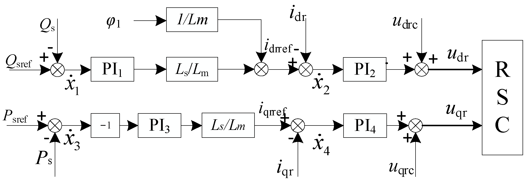
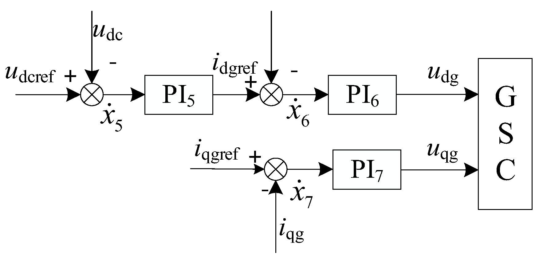
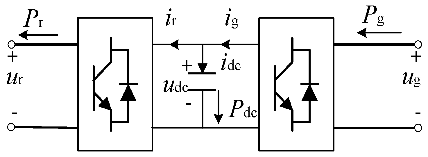
2.3. Converter and Control System Model

The main function of the rotor-side converter (RSC) is to control the current components of the d- and q-axes, thereby achieving decoupling control of active and reactive power. A dual closed-loop control based on the stator flux direction is adopted, where the d-axis controls the reactive power and the q-axis controls the active power. The specific control system structure is shown in Figure 3. Considering the intermediate variable ${\dot{x}}_1,{\dot{x}}_2,{\dot{x}}_3,{\dot{x}}_4$, the control system mathematical model of the RSC can be expressed in the form of differential equations as follows:

$$\left\{\begin{array}{l}{\displaystyle \frac{\mathrm{d}{x}_1}{\mathrm{d}t}}=Q_{\mathrm{ref}}-Q_{\mathrm{s}}\\ {\displaystyle \frac{\mathrm{d}{x}_2}{\mathrm{d}t}}={\displaystyle \frac{L_{\mathrm{s}}}{L_{\mathrm{m}}}}\left(k_{\mathrm{p}1}(Q_{\mathrm{ref}}-Q_{\mathrm{s}})+k_{\mathrm{i}1}{x}_1\right)-{\displaystyle \frac{{\phi }_1}{L_{\mathrm{m}}}}-i_{\mathrm{dr}}\\ {\displaystyle \frac{\mathrm{d}{x}_3}{\mathrm{d}t}}=P_{\mathrm{ref}}-P_{\mathrm{s}}\\ {\displaystyle \frac{\mathrm{d}{x}_4}{\mathrm{d}t}}={\displaystyle \frac{L_{\mathrm{s}}}{L_{\mathrm{m}}}}\left(k_{\mathrm{p}3}(P_{\mathrm{ref}}-P_{\mathrm{s}})+k_{\mathrm{i}3}{x}_3\right)-i_{\mathrm{qr}}\\ u_{\mathrm{dr}}=k_{\mathrm{p}2}\left({\displaystyle \frac{L_{\mathrm{s}}}{L_{\mathrm{m}}}}\left(k_{\mathrm{p}1}(Q_{\mathrm{ref}}-Q_{\mathrm{s}})+k_{\mathrm{i}1}{x}_1\right)-{\displaystyle \frac{{\phi }_1}{L_{\mathrm{m}}}}-i_{\mathrm{dr}}\right)\\ \hspace{1em} +k_{\mathrm{i}2}{x}_2+u_{\mathrm{drc}}\\ u_{\mathrm{qr}}=k_{\mathrm{p}4}\left({\displaystyle \frac{L_{\mathrm{s}}}{L_{\mathrm{m}}}}\left(k_{\mathrm{p}3}(P_{\mathrm{ref}}-P_{\mathrm{s}})+k_{\mathrm{i}3}{x}_3\right)-i_{\mathrm{qr}}\right)\\ \hspace{1em} +k_{i4}{x}_4+u_{\mathrm{qrc}}\end{array}\right.$$

(11)

where x₁ and x₃ represent intermediate variables introduced by the power control outer loop; and x₂ and x₄ denote intermediate variables from the rotor current control loop.

Wherein

$$\left\{\begin{array}{l}{u}_{\mathrm{drc}}=-({\omega }_{\mathrm{s}}-{\omega }_{\mathrm{r}})(L_r-{\displaystyle \frac{L_{\mathrm{m}}^2}{L_{\mathrm{s}}}})i_{\mathrm{qr}}\\ u_{\mathrm{qrc}}=({\omega }_{\mathrm{s}}-{\omega }_{\mathrm{r}})(L_r-{\displaystyle \frac{L_{\mathrm{m}}^2}{L_{\mathrm{s}}}})i_{\mathrm{dr}}+{\displaystyle \frac{L_{\mathrm{m}}}{L_{\mathrm{s}}}}({\omega }_{\mathrm{s}}-{\omega }_{\mathrm{r}}){\phi }_1\end{array}\right.$$

(12)

The control objective of the grid-side converter (GSC) is to maintain the constant direct current (DC) bus voltage and control the alternating current (AC) measurement power factor. The stability of the DC bus voltage is related to the AC measurement and the active power balance on the DC side, and the control of active power is actually the control of the current active component. Therefore, the control of the DC bus voltage is achieved on the d-axis. The grid-side vector control adopts a dual closed-loop control based on the voltage direction of the power grid, and its structure is illustrated in Figure 4.

Considering the intermediate variable, the mathematical model of the control system of the GSC can be expressed in the form of differential equations as follows:

$$\left\{\begin{array}{l}{\displaystyle \frac{\mathrm{d}{x}_5}{\mathrm{d}t}}=u_{\mathrm{dcref}}-u_{\mathrm{dc}}\\ {\displaystyle \frac{\mathrm{d}{x}_6}{\mathrm{d}t}}=k_{\mathrm{p}5}(u_{\mathrm{dcref}}-u_{\mathrm{dc}})+k_{\mathrm{i}5}{x}_5-i_{\mathrm{dg}}\\ {\displaystyle \frac{\mathrm{d}{x}_7}{\mathrm{d}t}}=i_{\mathrm{qgref}}-i_{\mathrm{qg}}\\ u_{\mathrm{dg}}=k_{\mathrm{p}6}\left[k_{\mathrm{p}5}(u_{\mathrm{dcref}}-u_{\mathrm{dc}})+k_{\mathrm{i}5}{x}_5-i_{\mathrm{dg}}\right]+\\ \hspace{1em}\hspace{1em}{k}_{i6}{x}_6\\ u_{\mathrm{qg}}=k_{\mathrm{p}7}(i_{\mathrm{qgref}}-i_{\mathrm{qg}})+k_{\mathrm{i}7}{x}_7\end{array}\right.$$

(13)

where x₅ corresponds to the intermediate variable in the voltage control loop, while x₆ and x₇ stand for intermediate variables introduced by the d-axis and q-axis current control loops of the grid-side converter, respectively.

When the loss of the converter is ignored, the power output from the rotor side of the DFIG is equal to the power transmitted to the grid through the GSC, thus maintaining a constant DC bus voltage u_dc. When the power on both sides is unequal, current flows through the capacitor branch and the DC bus voltage changes. The structure is depicted in Figure 5.

The dynamic process of the DC capacitor mentioned earlier can be described by the following differential equation:

$$\left\{\begin{array}{l}{P}_{\mathrm{g}}=P_{\mathrm{r}}+P_{\mathrm{dc}}\\ P_{\mathrm{dc}}=u_{\mathrm{dc}}{i}_{\mathrm{dc}}=C{u}_{\mathrm{dc}}{\displaystyle \frac{d{u}_{\mathrm{dc}}}{dt}}\end{array}\right.$$

(14)

Therefore,

$$C{u}_{\mathrm{dc}}{\displaystyle \frac{\mathrm{d}{u}_{\mathrm{dc}}}{\mathrm{d}t}}=u_{\mathrm{dg}}{i}_{\mathrm{dg}}+u_{\mathrm{qg}}{i}_{\mathrm{qg}}-u_{\mathrm{dr}}{i}_{\mathrm{dr}}-u_{\mathrm{qr}}{i}_{\mathrm{qr}}$$

(15)

Equation (5) describes the dynamic model equation of DFIG, Equation (10) describes the model equation of the speed control system under the power generation condition of the pump turbine, and Equations (11)–(15) describe the model equation of the doubly fed induction motor frequency converter and the control model equation of the frequency converter. By combining these equations, the dynamic model equation of DFIG-VSPS under power generation conditions can be obtained, and its state space expression is as follows:

$$\left\{\begin{array}{l}\dot{x}=f\left(x,y,u\right)\\ y=g\left(x,u\right)\end{array}\right.$$

(16)

where $x={\left[{\omega }_{\mathrm{m}} y h z {E^{\prime }}_{\mathrm{d}} {E^{\prime }}_{\mathrm{q}} i_{\mathrm{dr}} i_{\mathrm{qr}} x_1 x_2 x_3 x_4 u_{\mathrm{dc}} x_5 x_6 x_7\right]}^{\mathrm{T}}$ is the state variable, $y={\left[u_{\mathrm{dr}} u_{\mathrm{qr}} u_{\mathrm{dg}} u_{\mathrm{qg}}\right]}^{\mathrm{T}}$ is the output variable, and $u={\left[u_{\mathrm{ds}} u_{\mathrm{qs}} i_{\mathrm{dg}} i_{\mathrm{qg}}\right]}^{\mathrm{T}}$ is the input variable.

Combined with the contents described above, the overall control block diagram of the turbine of the doubly fed variable-speed pumped storage unit under working conditions can be obtained, and its structure is shown in Figure 6.

3. Small-Signal Model of the Single-Machine Infinite Bus System

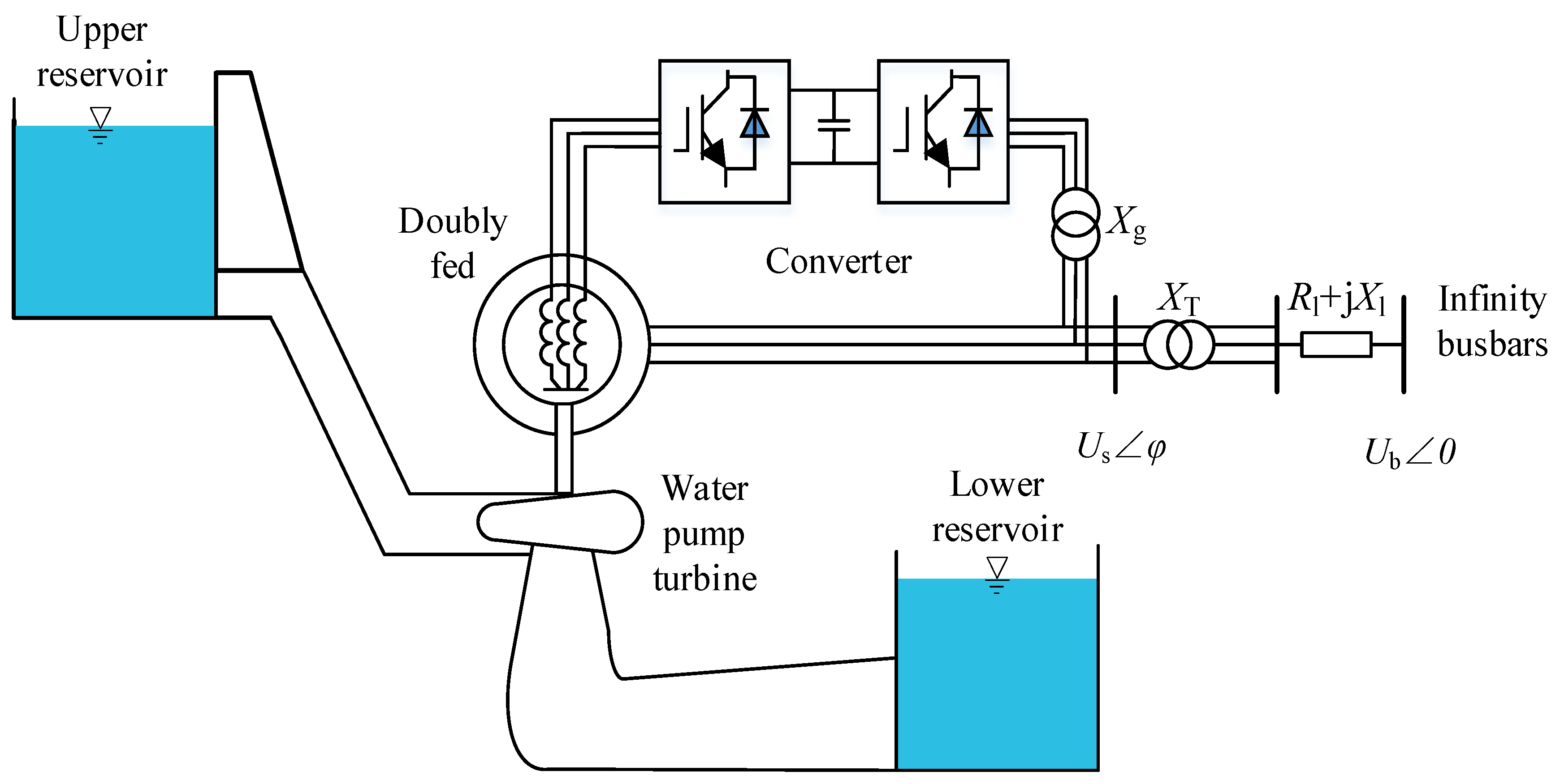
3.1. Single-Machine Infinite Bus System Model

The structural diagram of the connection of the DFIG-VSPS unit to the single-machine infinite bus system is shown in Figure 7.

The simple system of DFIG-VSPS primarily comprises a pump turbine, DFIG, step-up transformer, transmission line, and infinite bus system. The infinite bus system adopts an infinite bus with constant voltage amplitude and zero phase angle.

Ignoring the copper loss of the transformer and the resistance of the line, the voltage equation of the system shown in Figure 7 can be obtained as

$$U_{\mathrm{s}}\angle \phi =U_{\mathrm{b}}\angle 0+\mathrm{j}\left(X_{\mathrm{T}}+X_{\mathrm{l}}\right)\dot{I}\hspace{1em}=U_{\mathrm{b}}\angle 0+\mathrm{j}{X}_{\mathrm{L}}\left({\dot{I}}_{\mathrm{s}}+{\dot{I}}_{\mathrm{g}}\right)$$

(17)

where $X_{\mathrm{L}}=X_{\mathrm{T}}+X_{\mathrm{l}}$, $X_{\mathrm{T}}$ indicates the reactance of the step-up transformer and $X_{\mathrm{l}}$ indicates the reactance of the transmission line.

The voltage equation of Equation (17) was obtained in the α–β coordinate system. To be consistent with the previous model, it is necessary to transform it into the synchronous rotating d–q coordinate system. The voltage equation after transforming the coordinates is

$$\left[\begin{array}{c}{u}_{\mathrm{ds}}\\ u_{\mathrm{qs}}\end{array}\right]=\left[\begin{array}{c}\cos \phi \\ -\sin \phi \end{array}\right]U_{\mathrm{b}}+\left[\begin{array}{cc}0& -X_{\mathrm{L}}\\ X_{\mathrm{L}}& 0\end{array}\right]\left(\left[\begin{array}{c}{i}_{\mathrm{ds}}\\ i_{\mathrm{qs}}\end{array}\right]+\left[\begin{array}{c}{i}_{\mathrm{dg}}\\ i_{\mathrm{dg}}\end{array}\right]\right)$$

(18)

The voltage equation of the GSC is

$$\left[\begin{array}{c}{u}_{\mathrm{ds}}\\ u_{\mathrm{qs}}\end{array}\right]-\left[\begin{array}{c}{u}_{\mathrm{dg}}\\ u_{\mathrm{qg}}\end{array}\right]=\left[\begin{array}{cc}0& -X_{\mathrm{g}}\\ X_{\mathrm{g}}& 0\end{array}\right]\cdot \left[\begin{array}{c}{i}_{\mathrm{dg}}\\ i_{\mathrm{qg}}\end{array}\right]$$

(19)

3.2. Small-Signal Model for Simple Systems

The small-signal model considers that the deviation of the system’s operating state from the original equilibrium state after disturbance is extremely small. The process of linearizing the state equation of the system involves expanding the state equation of the system in a Taylor series at the original equilibrium state point and ignoring the second-order and higher terms of the deviation [18]. This linearized state equation is called the small model of the system. Based on the dynamic model equations obtained in Section 3.1 for DFIG-VSPS power generation conditions, the system is linearized at stable operating points, and the system state space expression obtained after linearization is solved. The linearized expressions of each differential equation are as follows, where $\Delta$ represents the increment of the variable at the stable operating point. Upon linearizing Equation (16), the following is obtained:

$$\left\{\begin{array}{l}{\displaystyle \frac{\mathrm{d}\Delta x}{\mathrm{d}t}}=A\Delta x+B\Delta y+B\Delta uC\\ {\displaystyle \frac{\mathrm{d}\Delta y}{\mathrm{d}t}}=D\Delta x+E\Delta u\end{array}\right.$$

(20)

The result of linearizing Equations (18) and (19) and solving them simultaneously can be expressed as

$$\Delta u=F\Delta x+G\Delta y$$

(21)

By introducing Equation (21) into Equation (20) and eliminating non-state variables, a simple system small-signal model for DFIG-VSPS can be obtained as follows:

$${\displaystyle \frac{\mathrm{d}\Delta x}{\mathrm{d}t}}=A_{sys}\Delta x$$

(22)

$A_{\mathrm{sys}}$ is called the state matrix of the system, and its size is a 16th-order square matrix.

4. Simple System Analysis

The eigenvalue method is used to analyze the small-disturbance stability of a simple system. Using the system parameters of the DFIG-VSPS unit, simulation verification was conducted to solve the eigenvalues and left and right eigenvectors of $A_{\mathrm{sys}}$. The absolute values of the real and imaginary parts of the eigenvalues, respectively, represent the damping and oscillation angle frequency of the corresponding mode. Using the Lyapunov stability criterion, the small-disturbance stability of the system can be determined based on the distribution of the eigenvalues on the complex plane.

Each real root of the feature matrix $A_{\mathrm{sys}}$ corresponds to a non-oscillatory mode. The specific correspondence is that the negative real root corresponds to the attenuation mode (AM), where the larger the absolute value, the faster the attenuation, while the positive real root corresponds to the amplification mode, where the larger the value, the more severe the instability of the system.

A pair of complex roots ${\lambda }_{\mathrm{i}}={\alpha }_{\mathrm{i}}+\mathrm{j}{\beta }_{\mathrm{i}}$ corresponds to an oscillation mode (OM), and the oscillation frequency and damping ratio can be determined using the following equations:

$$f_{\mathrm{i}}={\displaystyle \frac{{\beta }_{\mathrm{i}}}{2\pi }}$$

(23)

$$\xi ={\displaystyle \frac{-\alpha }{\sqrt{{\alpha }^2+{\beta }^2}}}$$

(24)

4.1. State Analysis of OM

Using MATLAB, a total of 16 eigenvalues of the state matrix were solved, and the corresponding damping ratios were calculated, as listed in

Table 1. Calculation results of characteristic values.

Mode	Order	Eigenvalue	Damping Ratio
OM1	λ1,2	–5.443 ± 29.157	0.184
OM2	λ3,4	–1.879 ± 3.943	0.430
OM3	λ5,6	–0.128 ± 0.896	1.141
OM4	λ7,8	–0.195 ± 2.166	0.090
OM5	λ9,10	–0.377 ± 0.710	0.468
AM1	λ11	–63.192	1
AM2	λ12	–7.689	1
AM3	λ13	–5.818	1
AM4	λ14	–1.401	1
AM5	λ15	–0.580	1
AM6	λ16	–0.560	1

Note: OM, oscillation mode; AM, attenuation mode.

.

The conjugate eigenvalues with negative real parts indicate that the unit will undergo a decaying oscillation process and become stable after being subjected to small disturbances, which is called the OM. Real eigenvalues with negative real parts indicate that the system tends to stabilize without undergoing an oscillation process after being subjected to small disturbances; this is known as the AM.

From Table 1, it can be observed that all characteristic roots of the system are negative real numbers or have negative real parts, indicating that the OM of the system is in decay, which means that the system is stable with small disturbances. Over time, the system will return to the equilibrium point before the small disturbance occurs. The simple DFIG-VSPS system contains five pairs of OMs and six AMs. Except for OM4 corresponding to eigenvalues λ₇ and λ₈, which has a relatively low damping ratio of 0.090, the damping ratios of the other four OMs are 0.184, 0.430, 0.141, and 0.468, respectively. These OMs all have suitable damping ratios, satisfying the requirement of a damping ratio greater than 0.05 during stable system operation [19].

4.2. Interactions Between State Variables

The interaction between state variables was studied through the participation factor method. The calculation expression is

$$P_{ki}=\left|{\displaystyle \frac{V_{ki}{U}_{ki}}{V_i^{\mathrm{T}}{U}_i}}\right|,$$

(25)

where P_ki indicates the degree of influence of state variable k on mode i, and V_ki and U_ki are the k-th state variable elements in the left and right eigenvectors of the system state matrix under mode i, respectively [20]. The participation factors of the system modes can be calculated using Equation (25), as listed in

Table 2. Participation factors corresponding to each state variable.

Variable	λ1 λ2	λ3 λ4	λ5 λ6	λ7 λ8	λ9 λ10	λ11	λ12	λ13	λ14	λ15	λ16
∆ωm	0.01	0	0	0.18	0.34	0.01	0.01	0	0	0.15	0
∆y	0.01	0	0	0.15	0.26	0.67	0.02	0	0	0.01	0
∆h	0.01	0	0	0.11	0.24	0.32	0.02	0	0	0	0
∆z	0	0	0	0.01	0.02	0	0	0	0	0.83	0
$\Delta E_{\mathrm{d}}^{\prime }$	0.05	0	0.02	0.22	0.05	0	0.01	0.01	0.01	0	0
$\Delta E_{\mathrm{q}}^{\prime }$	0	0	0.02	0.22	0.04	0	0	0.03	0.07	0	0.03
∆idr	0	0	0	0.03	0.01	0	0	0.74	0.18	0	0.03
∆iqr	0.45	0	0.01	0.04	0.01	0	0.07	0.01	0	0	0
∆x1	0	0	0	0	0	0	0	0.08	0.17	0	0.8
∆x2	0	0	0	0	0	0	0	0.14	0.57	0	0.12
∆x3	0.36	0	0	0	0	0	0.1	0	0	0	0
∆x4	0.12	0	0	0	0	0	0.77	0	0	0	0
∆udc	0	0.03	0.45	0.02	0.01	0	0	0	0	0	0
∆x5	0	0.05	0.45	0.02	0.01	0	0	0	0	0	0
∆x6	0	0.46	0.02	0	0	0	0	0	0	0	0
∆x7	0	0.46	0.02	0.01	0	0	0	0	0	0	0

Note: The variables in the table are the variables after linearization of the corresponding variables, with the highlighted participation factors indicating the dominant state variables in the corresponding AM or OM

.

The participation factors listed in Table 2 clearly reflect the degree of participation of all state variables in each OM.

We first analyzed the dominant state variables in five OMs. OM1 (λ₁ and λ₂) is affected by the variation values ∆i_qr, ∆x₄ of the rotor q-axis current, and the deviation value ∆x₃ of the active power. It is strongly related to the control system of the RSC, and as a result, the parameters of the rotor-side power outer loop and current inner loop controller affect this mode.

The dominant state variable of OM2 (λ₃ and λ₄) indicates the $d$- and $q$-axis current difference ∆x₆ and ∆x₇ of the current inner loop in the GSC control system. Therefore, the controller parameters of the grid-side converter current inner loop have an impact on this OM. Additionally, the participation factor also reflects that this mode is not related to the relevant state variables of the pump turbine and DFIG.

The dominant state variables of OM3 (λ₅ and λ₆) are the variation value of the DC voltage ∆u_dc and the deviation value of the DC link voltage ∆x₅. Therefore, it is primarily related to the voltage variation on the DC side of the converter and is inevitably affected by the external control parameters of the GSC voltage. Maintaining a constant DC side voltage can effectively suppress OM3, and this OM is not related to the state variables of the pump turbine speed control system.

Numerous state variables affect OM4 (λ₇ and λ₈), among which the most dominant is the speed change value ∆ω_m, followed by the opening change value ∆y, water head change value ∆h, and transient electromotive force change of the motor ΔE^′_d and ΔE^′_q; therefore, this mode is associated with the parameters of the speed control system of the pump turbine, the operating status of the unit, and the parameters of the DFIG.

OM5 (λ₉ and λ₁₀) is affected by the speed change value ∆ω_m. The joint influence of the head change value ∆h and the opening change value ∆y is primarily related to the parameters of the pump turbine speed control system and the operating state of the unit and is unaffected by the state variables related to the DFIG and the converter controller system.

For the six AMs in the system, the attenuation process from AM1 to AM3 is faster and has less impact on the small-disturbance stability of the system. The attenuation process of AM4, AM5, and AM6 is relatively slow, with AM4 and AM6 having the strongest correlation with the changes in stator reactive power ∆x₁ and stator d-axis current ∆x₂. AM5 has the highest correlation with the changes in pump turbine speed ∆ω_m and ∆z.

4.3. Influence of System Parameters on Feature Roots

Further investigation was undertaken based on the calculation results of the participation factors to verify the relationship between the system OMs and state variables in Section 4.2 and to study the trend of system stability changes when parameters change. By changing certain parameters of the pump turbine and DFIG control system, the characteristic root change trajectories of OMs with high correlation with these parameters were studied, and the impact on system stability was analyzed.

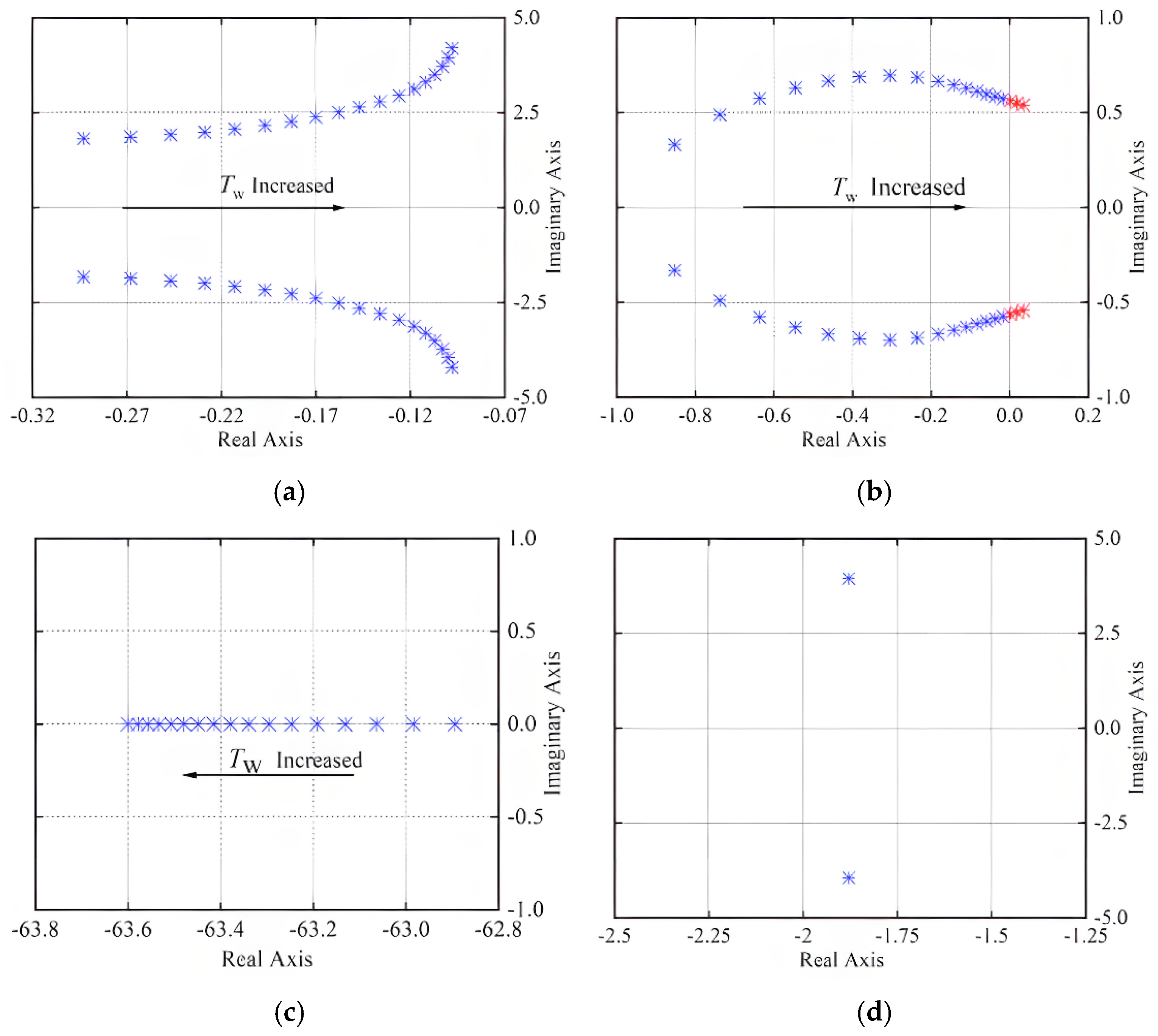
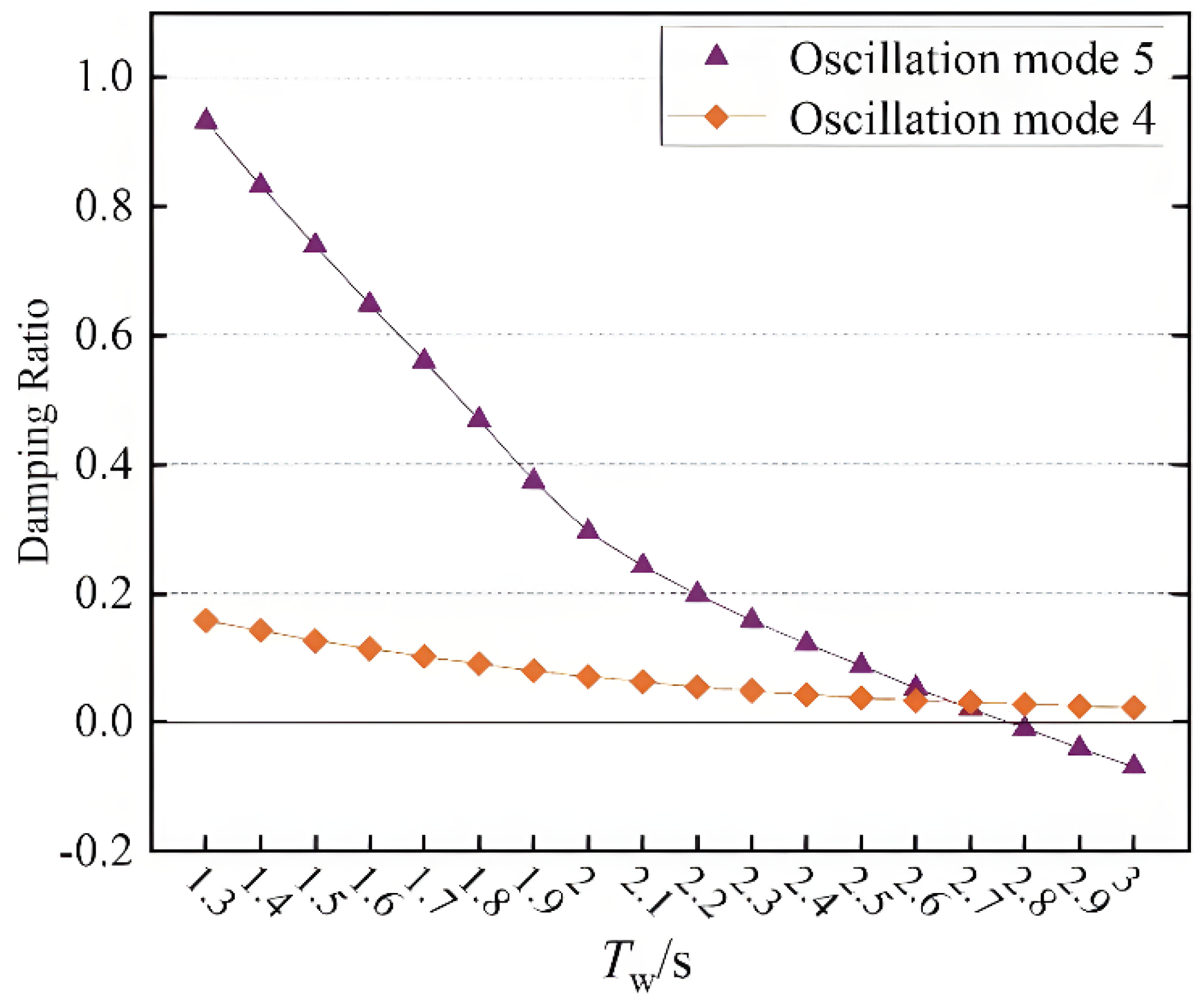
4.3.1. Changing the Inertia Time Constant T_w of Water Flow

Referring to relevant information, the inertia time constant T_w of mixed flow units is primarily concentrated between 0.8 and 4.0 s, and the calculated value in this study is T_w = 1.8 s. The different values of T_w have a significant impact on the state variables related to the water diversion system. According to the analysis in Section 4.2, the modes with a strong correlation with the state variables of the water diversion system primarily include OM4, OM5, and AM1. To verify the correctness of the conclusions drawn based on the participation factor and to study the impact of the water flow inertia time constant T_w on the small-disturbance stability of the system, the trajectories of the eigenvalues of the four modes on the complex plane are illustrated in Figure 8 during the process of increasing T_q values from 1.3 to 3.0 s, taking OM4, OM5, AM1, and OM2 with a participation factor of zero with the water diversion system state variable as the objects.

Figure 8 illustrates that the characteristic roots of OM4, OM5, and AM1, which have a strong correlation with the state variables of the water diversion system, change with the increase in T_w. This change is reflected in the complex plane being close to or far from the imaginary axis. The eigenvalues of OM2 with a participation factor of zero for the state variable of the water diversion system are unaffected by changes in the value of T_w, which also proves that the relevant state variables of the water diversion system do not participate in OM2, which is consistent with the conclusions drawn based on the participation factor in Section 4.2.

In addition, as T_w increases, the eigenvalues of OM4 and OM5 gradually approach the imaginary axis, whereas the eigenvalues of AM1 move farther from the imaginary axis, indicating that increasing T_w can accelerate the attenuation speed of AM1. However, the amplitude of the change in the eigenvalues of AM1 is relatively small and far from the imaginary axis, which has little impact on the small-disturbance stability of the system. Figure 9 illustrates the damping ratios of OM4 and OM5 as a function of T_w. When T_w increases from 1.3 to 3.0 s, the damping ratio of OM4 decreases from 0.158 to 0.023, and the damping ratio of OM5 decreases from 0.932 to 0.021. Until T_w = 2.8 s, the characteristic roots of OM5 show positive real parts, and the system shows negative damping. This mode changes from attenuated oscillation to amplified oscillation, indicating that the system is unstable with small disturbances at this time. It can be observed that as the water flow inertia time constant T_w increases, the damping characteristics of the entire system deteriorate, and the small-disturbance stability gradually weakens. An excessive water flow inertia time constant may make the system unstable.

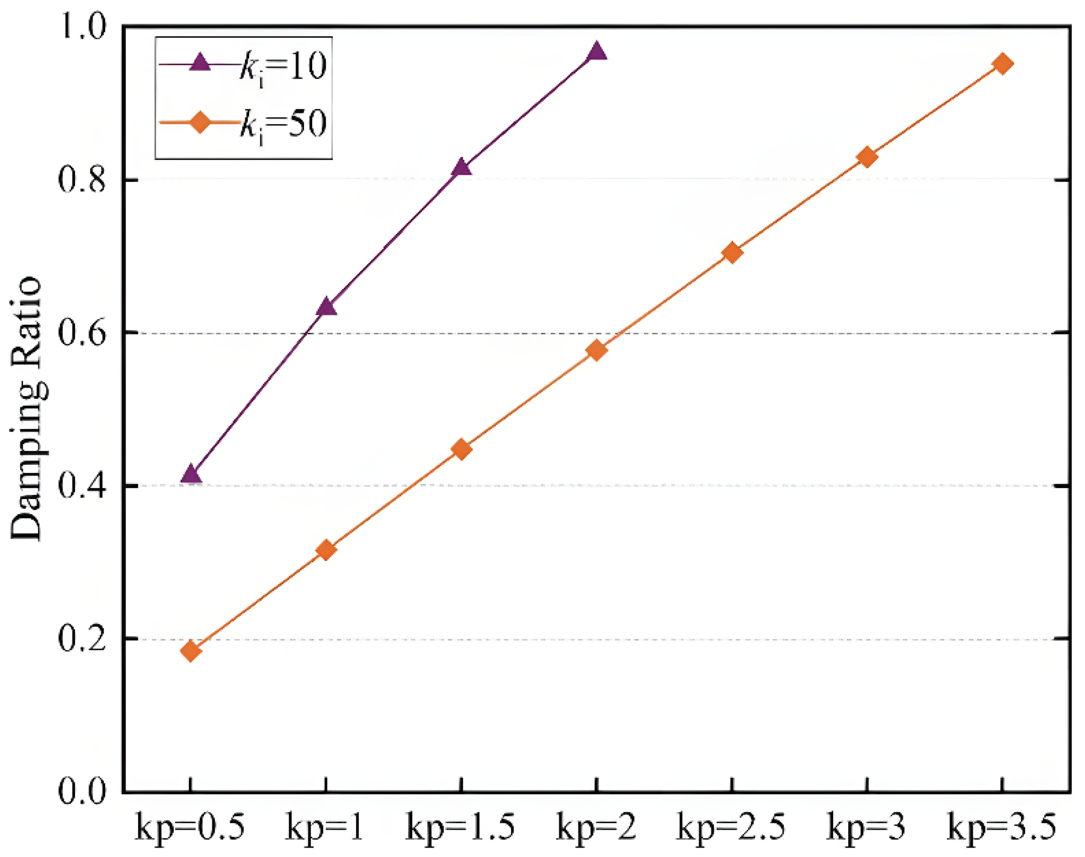
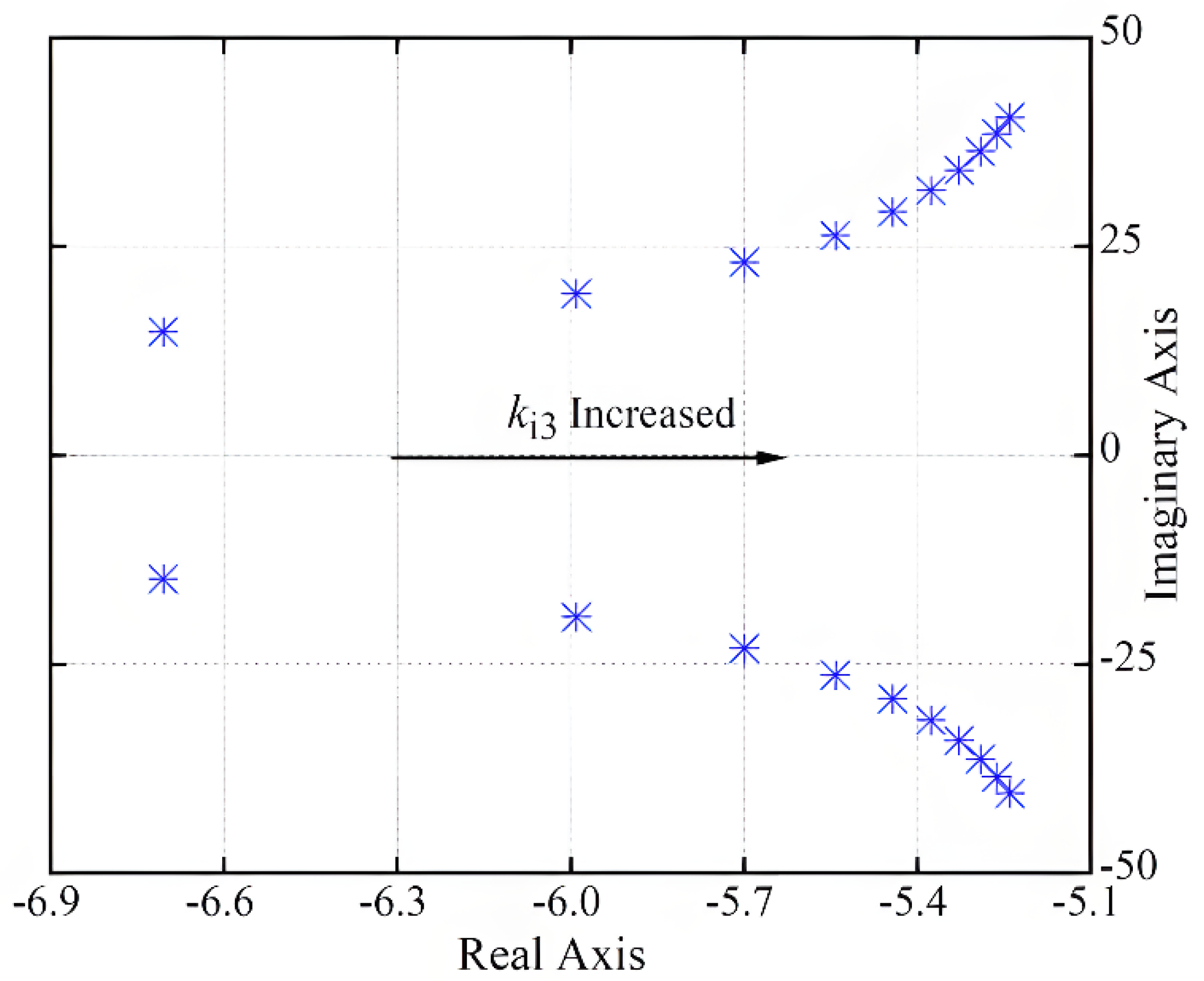
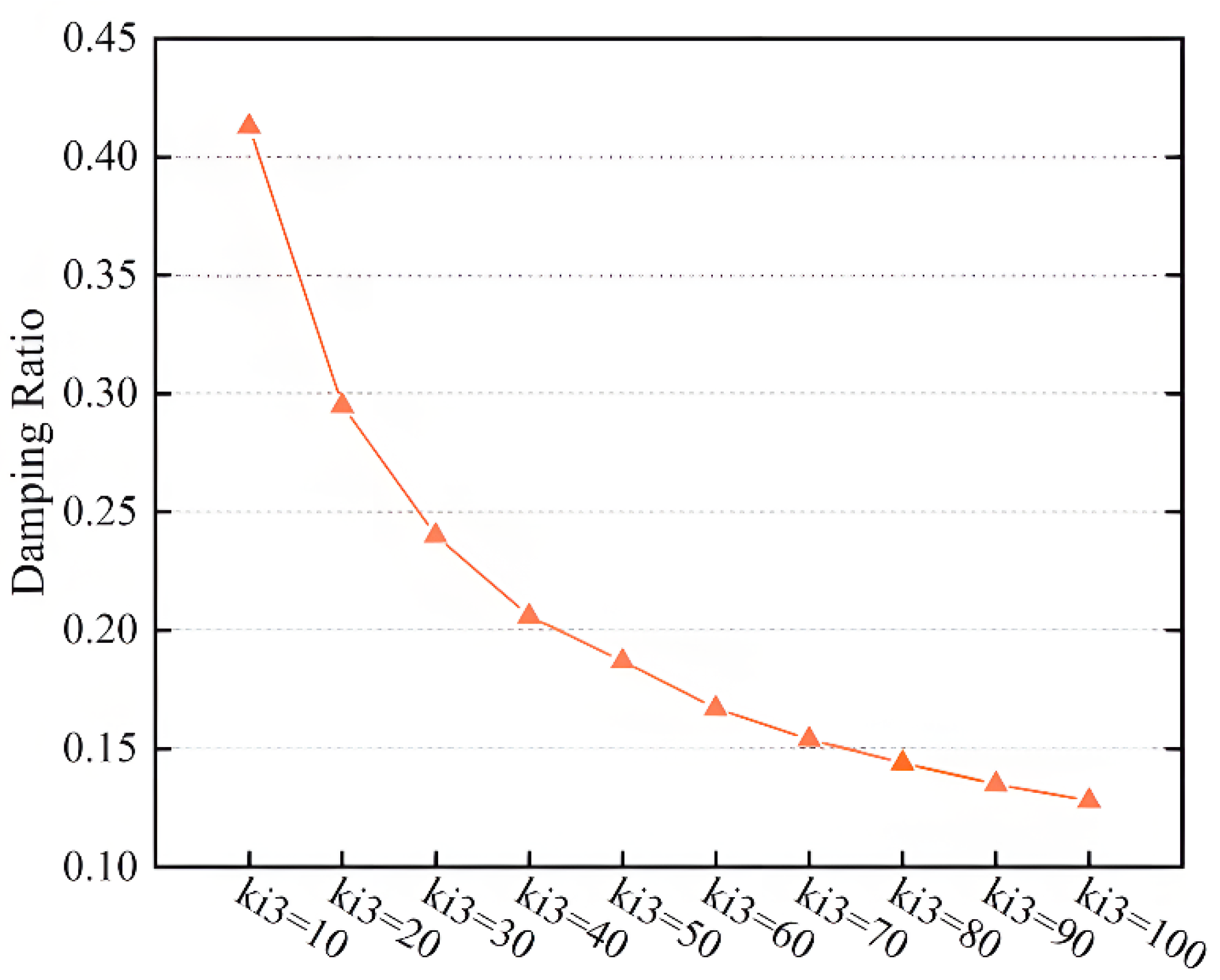
4.3.2. Changing the Control Parameters of the Converter

Based on the results of the factor analysis in Section 4.2, it can be observed that OM1 is affected by the control parameters of the power outer loop and current inner loop of the RSC. Therefore, k_i3 = 10 and k_i3 = 50 were taken, respectively, and k_p3 gradually increased from 0.5 to 6. The trajectory of the eigenvalues of OM1 on the complex plane is shown in Figure 10.

Figure 10 shows that when k_i3 is constant, as k_p3 increases, the characteristic roots of OM1 move away from the imaginary axis, indicating that the damping ratio of the system increases, and the stability of the system is enhanced. The variation of damping ratio is shown in Figure 11.

When k_i3 = 10, during the process of increasing k_p3 from 0.5 to 2, the damping ratio increases from 0.413 to 0.966 and then continues to increase with increasing k_p3. OM1 transitions into two AMs; when k_i3 = 50, during the process of increasing k_p3 from 0.5 to 3.5, the damping ratio increases from 0.184 to 0.952 and then continues to increase with increasing k_p3.

Additionally, this OM will transition into two AMs. Based on this, the following conclusion can be drawn: when k_i3 is constant, appropriately increasing the outer loop controller parameter k_p3 of the RSC power can significantly improve the damping characteristics of the system, transition the OM to AM, and thus improve the small-disturbance stability of the system.

Furthermore, by comparing the damping changes when k_i3 = 10 and k_i3 = 50 in Figure 11, it can be observed that the value of k_i3 also affects the damping ratio of the system. Therefore, to study the relationship between the value of k_i3 and system stability, while keeping k_p3 unchanged and increasing k_i3 from 10 to 100, the eigenvalue trajectory of OM1 is shown in Figure 12.

The variation of damping ratio is shown in Figure 13.

Figure 12 and Figure 13 show that when k_p3 remains constant and k_i3 increases, the characteristic roots of OM1 move toward the imaginary axis, indicating a decrease in the damping ratio of this mode and a decrease in system stability. Specifically, when k_p3 = 0.5, k_i3 increased from 10 to 100, and the damping ratio decreased from 0.413 to 0.128. Once k_i3 exceeded 50, the decreasing trend of the further increasing k_i3 damping ratio gradually weakened.

5. Simulation Verification

To verify the correctness of the analysis presented in Section 4, we constructed an electromagnetic transient model of the DFIG-VSPS under power generation conditions based on MATLAB/Simulink. By providing power disturbances and simulating small-disturbance signals during system operation, we observed whether the unit can transition from the current state to a new stable state and verified the small-disturbance stability of the system and the impact of parameter changes on system stability.

5.1. Impact of Water Flow Inertia Time Constant T_w

The simulation settings were as follows. At the initial moment, the output of the DFIG-VSPS was 0.8 pu, the head 1.0 was $\mathrm{pu}$, and the speed was 0.955 pu. At 70 s, the power reference value stepped from 0.8 pu to 0.7 $\mathrm{pu}$. The simulation results of the unit speed at T_w = 2.0, 2.3, and 2.6 s were obtained, as shown in Figure 14.

The simulation results show that under the three tested values of T_w, the unit can transition to a new stable state after being subjected to small disturbances in the power step, indicating that the system satisfies the requirements of small-disturbance stability. However, as T_w increased, the speed of the oscillation attenuation slowed, and the time required to recover to a stable state increased, indicating that the damping of the system gradually decreased, and the stability of the entire system weakened. This is consistent with the results of the eigenvalue root trajectory analysis presented in Section 4.3, indicating the accuracy of the theoretical analysis.

Figure 15 presents the simulation results when T_w continues to increase to 2.8 s.

At this point, the oscillation speed increased, and as time progressed, the oscillation amplitude increased. The system cannot transition to a new stable state, resulting in instability. The system did not satisfy the requirements for small-disturbance stability, which is consistent with the conclusions presented in Section 4.3.1. As T_w increases, there exists a risk of instability in the system.

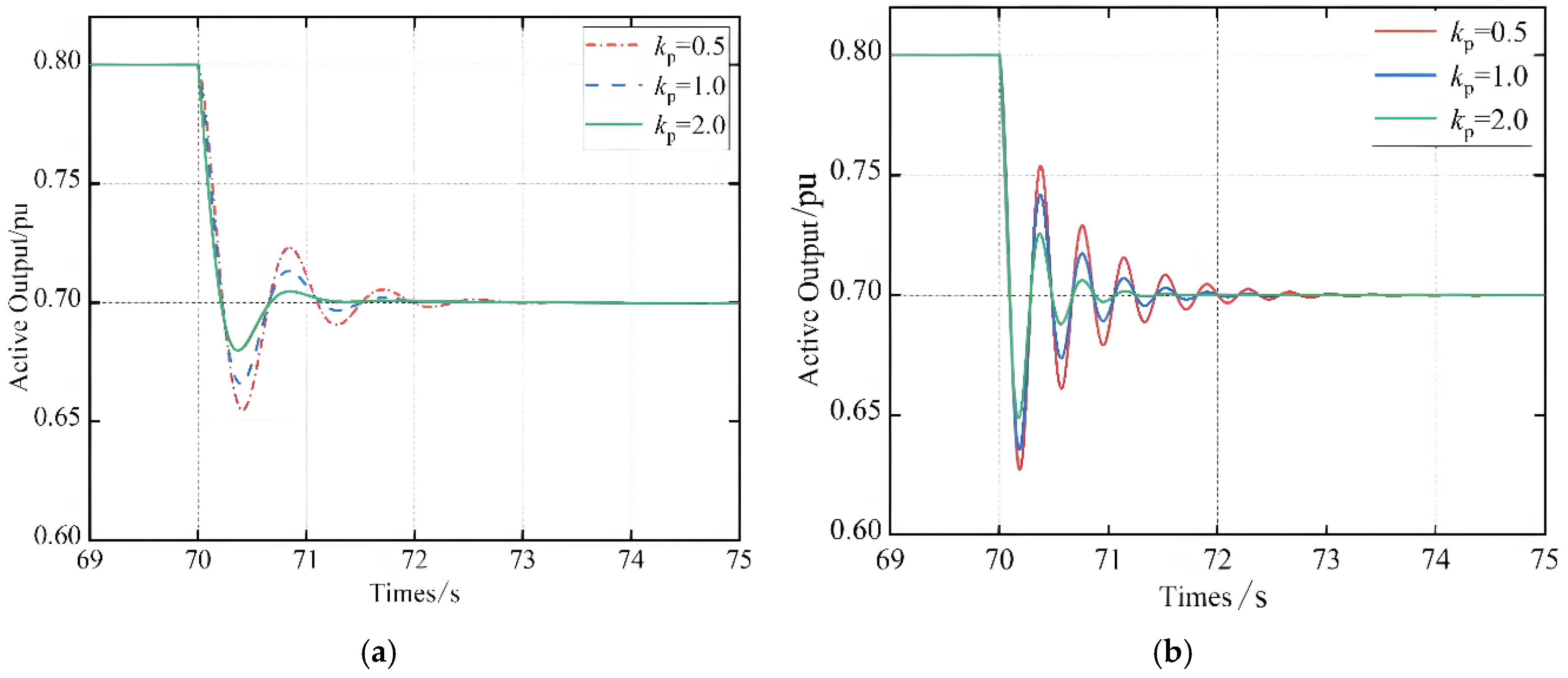
5.2. Influence of the Control Parameters of the RSC

The time–domain simulation conditions were set as described in the previous section, with k_i3 = 10 and 100. Figure 16 illustrates the system power output response during the process of increasing k_p3 from 0.5 to 2.

Figure 16 illustrates that increasing the value of k_p3 can reduce the number and amplitude of oscillations while keeping k_i3 constant and enable the system to transition to a new stable state more quickly. Therefore, increasing k_p3 has a significant inhibitory effect on the oscillation, which can enhance the damping of the system and make it more stable. As k_i3 increased, the number of oscillations increased, and the time required for the system to recover its stability increased. Therefore, an increase in k_i3 deteriorated the OM of the system and reduced its damping. This is consistent with the conclusion drawn from the root trajectory analysis presented in Section 4.3, which verifies the accuracy of the root trajectory analysis.

6. Small Signal Stability Analysis of Interconnected Systems with DFIG-VSPS

Variable-speed pumped storage units serve as flexible and efficient regulation tools in power grids, playing a vital role in peak shaving and frequency regulation across regional power networks. However, interconnected power systems often exhibit weakly damped oscillation modes that may trigger system oscillations under disturbances, thereby affecting the small signal stability of interconnected systems. As a new type of power station, the impact of doubly fed induction generator-based variable-speed pumped storage (DFIG-VSPS) on the original oscillation modes of interconnected systems remains unclear. This chapter therefore investigates variations in damping ratios and oscillation frequencies of key oscillation modes in the original system when DFIG-VSPS is connected at different locations and through different integration approaches, based on a four-machine two-area interconnected system model.

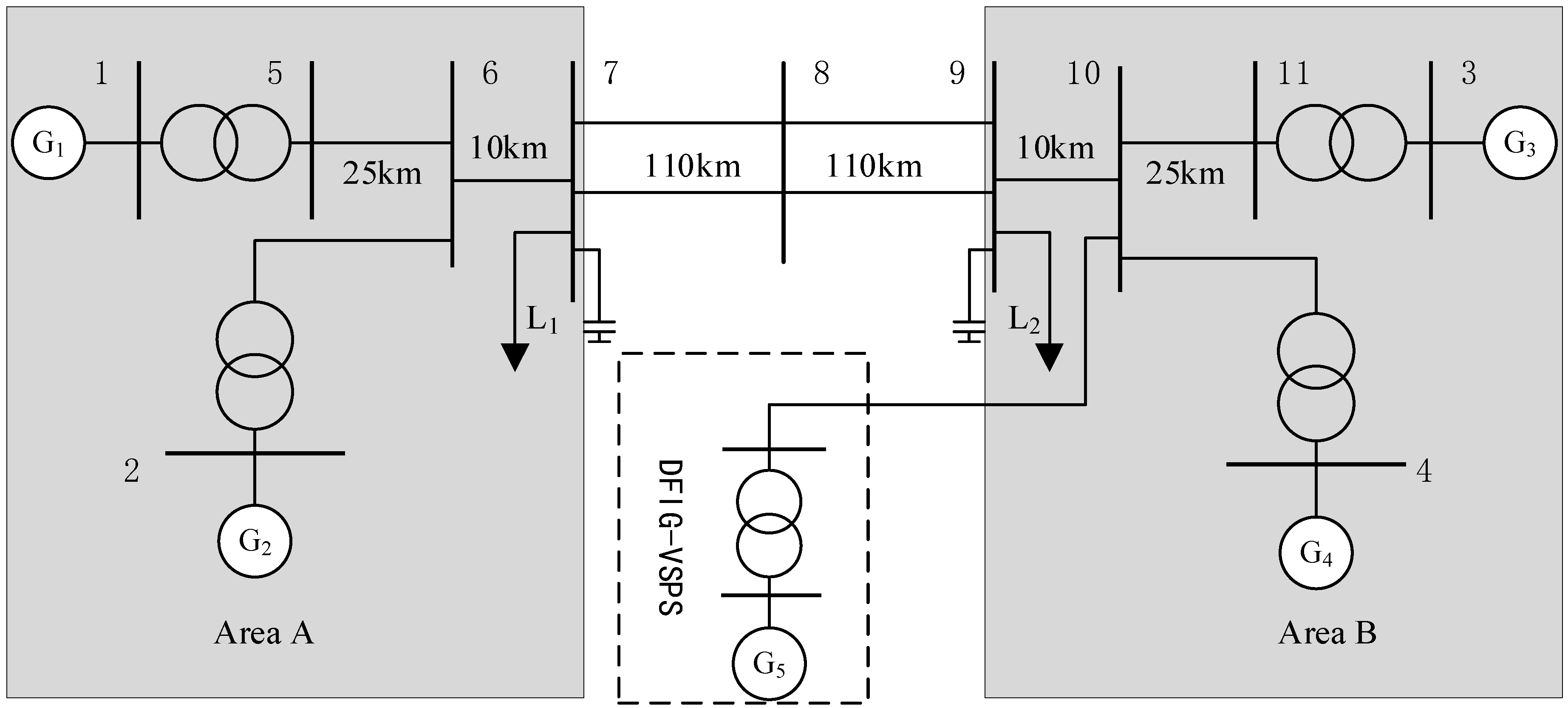
6.1. Four-Machine Two-Area System Model

The classic IEEE four-machine two-area system is widely used in small signal stability analysis of power systems. The structure of the doubly fed variable-speed pumped storage unit integrated into the four-machine two-area system is shown in Figure 17. The entire system is divided into Area A and Area B, each containing two identical synchronous generators (G1 and G2 in Area A, G3 and G4 in Area B). The two areas are connected via a tie-line between Bus 7 and Bus 9 to enable power transmission. An active load L1 of 967 MW and a reactive load of 100 Mvar are connected at Bus 7, while an active load L2 of 1767 MW and a reactive load of 100 Mvar are connected at Bus 9. Area A delivers 210 MW of active power to Area B. The lengths of the transmission lines are provided in Figure 17, with a line resistance of 0.0529 Ω/km and a line reactance of 0.0529 Ω/km.

The four synchronous generator units each have a nominal apparent power of 900 MVA and a nominal voltage of 20 kV. The active power output of G1, G2, and G4 is set to 700 MW with a power factor of 0.8. G1 is designated as the balance machine with its power factor set to 0.9. The synchronous generators adopt a fifth-order model, with the specific parameters provided in

Table 3. Parameters of synchronous motors.

Parameter	G1, G2	G3, G4
$X_{\mathrm{d}}$/pu	1.8	1.8
$X_{\mathrm{q}}$/pu	1.7	1.7
$X_{\mathrm{d}}^{\prime }$/pu	0.3	0.3
$X_{\mathrm{q}}^{\prime }$/pu	0.55	0.55
$X_{\mathrm{d}}^{″}$/pu	0.25	0.25
$X_{\mathrm{q}}^{″}$/pu	0.25	0.25
$T_{\mathrm{d}}^{\prime }$/s	8	8
$T_{\mathrm{q}}^{\prime }$/s	0.4	0.4
$T_{\mathrm{d}}^{″}$/s	0.03	0.03
$T_{\mathrm{q}}^{″}$/s	0.05	0.05
$H_{\mathrm{g}}$/pu	6.5	6.175

.

6.2. Eigenvalue Analysis of the System Before and After DFIG-VSPS Integration

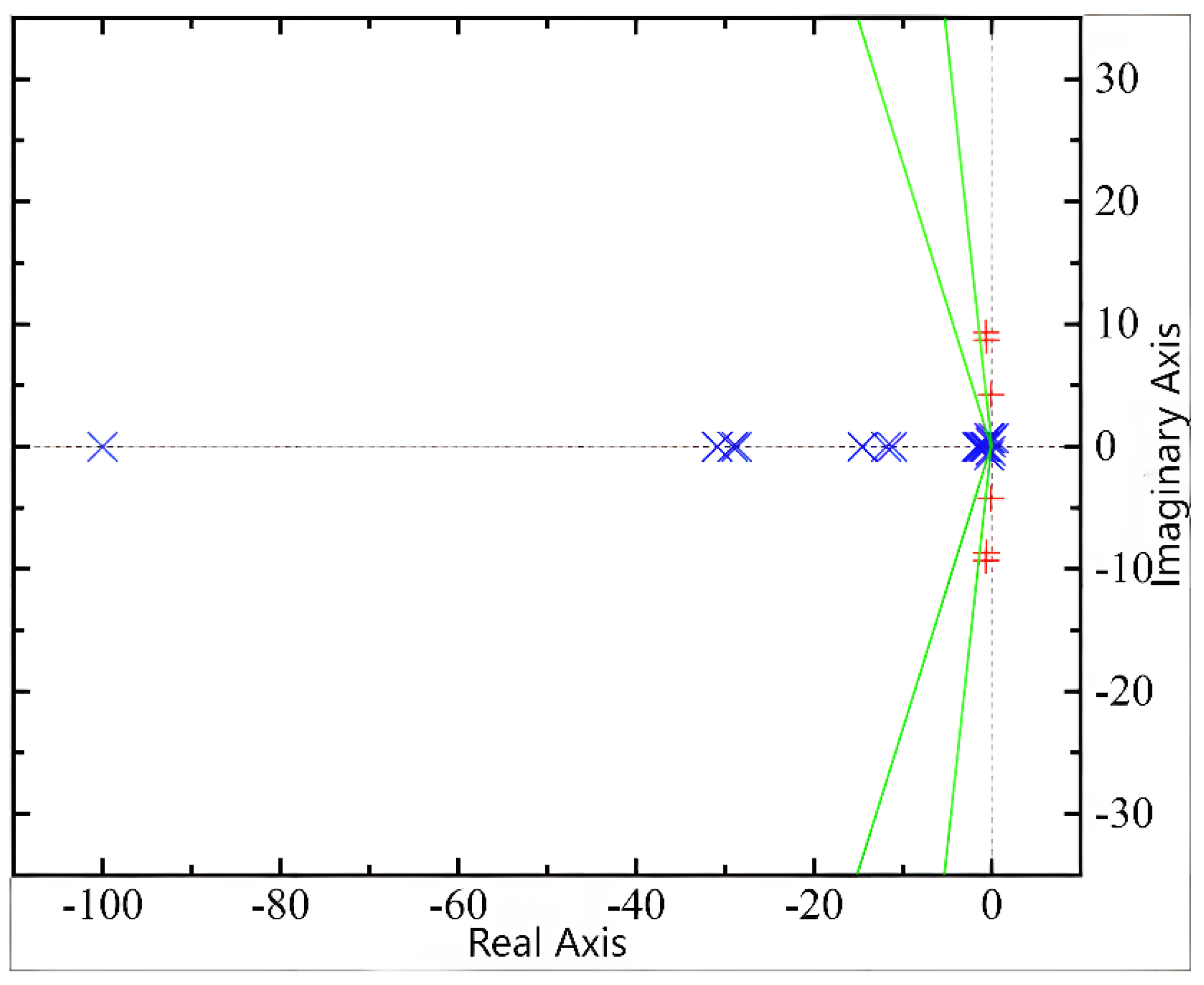
6.2.1. Eigenvalue Analysis of the Four-Machine Two-Area System

To assess the impact of doubly fed induction generator-based variable-speed pumped storage (DFIG-VSPS) integration on small signal stability, eigenvalue calculations were performed for the system both before and after DFIG-VSPS integration. Prior to DFIG-VSPS integration, the distribution of eigenvalues for the four-machine two-area system in the complex plane is illustrated in Figure 18, where the diagonal lines represent constant damping ratio lines of 0.4 and 0.15 (from left to right).

As shown in the figure, all system eigenvalues are located in the left half-plane, indicating that the system meets small signal stability requirements. However, three sets of oscillatory mode eigenvalues (highlighted in red) are positioned to the right of the 0.15 constant damping ratio line, exhibiting relatively low damping ratios. These represent the system’s critical oscillatory modes. These three eigenvalue sets were extracted for further analysis, with their damping ratios and oscillation frequencies calculated. Through participation factor analysis, the synchronous generator units associated with each mode were identified, with the results presented in

Table 4. Key oscillation modes of the four-machine two-area system.

Oscillation Mode	Eigenvalue	Damping Ratio	Oscillation Frequency/HZ	Relevant Generating Units
1	−0.595 ± j8.671	0.068	1.380	G1, G2
2	−0.658 ± j9.321	0.070	1.483	G3, G4
3	−0.081 ± j4.237	0.019	0.674	G1, G2, G3, G4

.

As evidenced by the table, Oscillation Mode 1 is predominantly influenced by state variables from synchronous machines G1 and G2 in Area A, manifesting as relative oscillations between G1 and G2. This is identified as a local oscillation mode within Area A. Similarly, Oscillation Mode 2 represents a local oscillation pattern within Area B.

The two local oscillation modes exhibit damping ratios of 0.068 and 0.070, respectively, with oscillation frequencies of 1.380 Hz and 1.483 Hz—both falling within the range of low-frequency oscillations characteristic of power systems.

Oscillation Mode 3 demonstrates participation from state variables of all four synchronous machines, exhibiting relative oscillations between Area A and Area B, thus classified as an inter-area oscillation mode. With an oscillation frequency of 0.674 Hz (also within the low-frequency range) and a damping ratio of 0.019, this mode qualifies as a weakly damped oscillation. Crucially, Mode 3 represents the key factor affecting small signal stability in the four-machine two-area system.

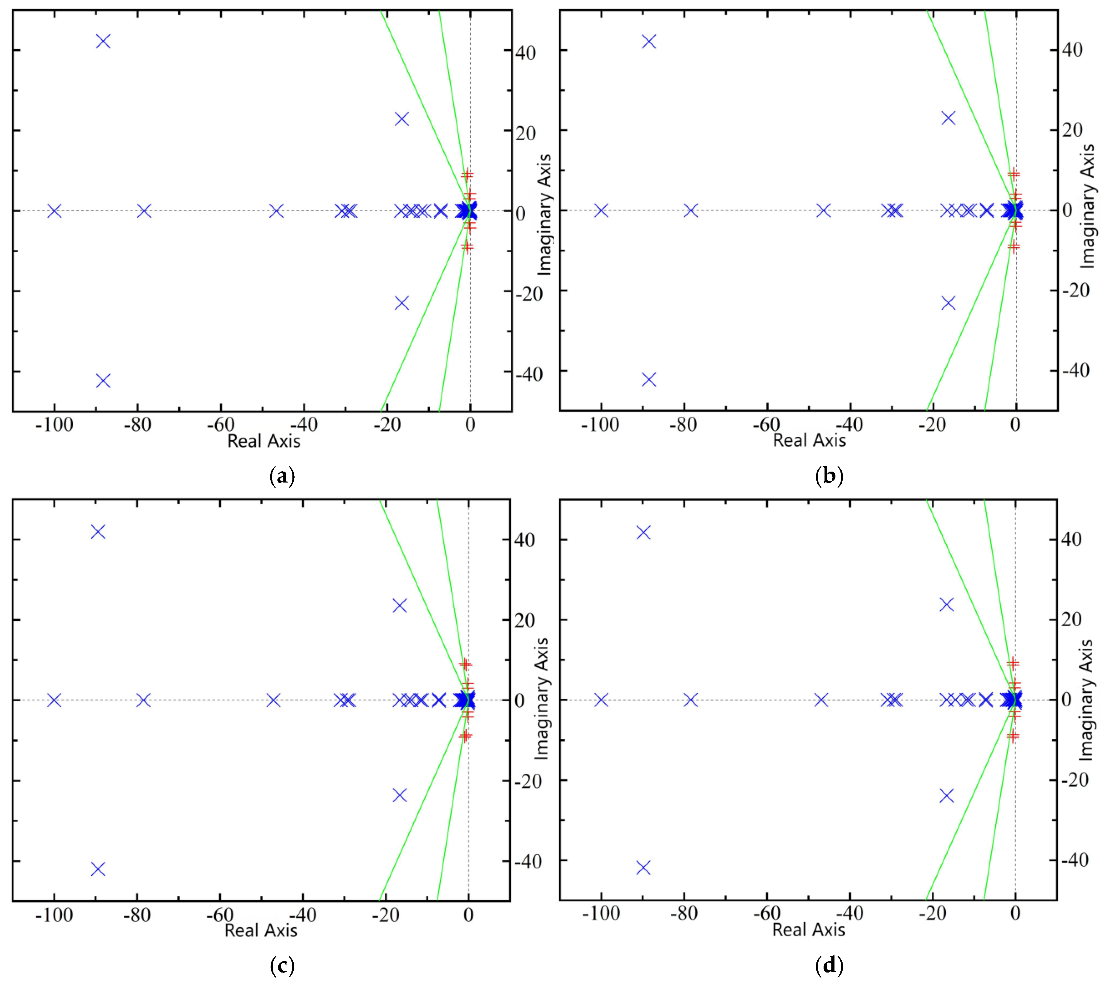
6.2.2. Eigenvalue Analysis of the System After DFIG-VSPS Integration

In the four-machine two-area system, Area A transmits 210 MW of active power to Area B, making Area A the power-sending region and Area B the power-receiving region. The doubly fed variable-speed pumped storage (DFIG-VSPS) unit can be connected to either the sending end Area A or the receiving end Area B. After integration, the DFIG-VSPS can maintain system power balance by either increasing the load within the connected area or reducing the output of synchronous generators in that area.

A 400 MW DFIG-VSPS unit is integrated into the four-machine two-area system while maintaining the 210 MW power transfer from Area A to Area B. Four different scenarios are established to study the impact of DFIG-VSPS integration on the small signal stability of the interconnected system. The scenarios are configured as follows:

Scenario 1: the DFIG-VSPS is connected to Bus 6 in sending end Area A, while the output of synchronous generator G2 is reduced by 400 MW.

Scenario 2: the DFIG-VSPS is connected to Bus 6 in sending end Area A, while an additional 400 MW active load is added in Area A.

Scenario 3: the DFIG-VSPS is connected to Bus 10 in receiving end Area B, while the output of synchronous generator G4 is reduced by 400 MW.

Scenario 4: the DFIG-VSPS is connected to Bus 10 in receiving end Area B, while an additional 400 MW active load is added in Area B.

The distribution of eigenvalues in the complex plane for these four scenarios after DFIG-VSPS integration is shown in Figure 19, where the diagonal lines represent constant damping ratio lines of 0.4 and 0.15 (from left to right).

Initial observation of Figure 19 reveals that in all four scenarios following DFIG-VSPS integration into the four-machine two-area system, all system eigenvalues remain distributed in the left half-plane, confirming that the system maintained small signal stability. A comparative analysis between Figure 18 and Figure 19 demonstrates that the four scenarios in Figure 19 exhibit increased quantities of both real and complex conjugate eigenvalues, indicating that the doubly fed variable-speed pumped storage unit introduces new oscillatory and decaying modes to the system. However, most newly introduced oscillatory modes are situated to the left of the 0.4 constant damping ratio line, exhibiting relatively high damping ratios characteristic of strongly damped modes that do not critically determine small signal stability. Notably, the DFIG-VSPS integration does not substantially alter the original eigenvalue distribution pattern of the four-machine two-area system, with pre-existing oscillatory modes persisting post-integration. The final comparison of the four subplots in Figure 19 shows fundamentally similar eigenvalue distribution patterns across all scenarios, with each case featuring one additional oscillatory mode appearing to the right of the 0.15 damping ratio line (with relatively low damping) that combines with the system’s original three oscillatory modes to form the post-integration critical oscillatory modes (highlighted in red). The damping ratios, oscillation frequencies, and associated generator units for these four critical oscillatory modes are detailed in

Table 5. The key oscillation modes of the system in four scenarios.

	Oscillation Mode	Eigenvalue	Damping Ratio	Oscillation Frequency/HZ	Relevant Generating Units
Four-Machine Two-Area System	1	−0.595 ± j8.671	0.068	1.380	G1, G2
	2	−0.658 ± j9.321	0.070	1.483	G3, G4
	3	−0.081 ± j4.237	0.019	0.674	G1, G2, G3, G4
Scenario 1	1	−0.857 ± j8.659	0.098	1.378	G1, G2
	2	−0.659 ± j9.321	0.070	1.483	G3, G4
	3	−0.091 ± j4.218	0.022	0.671	G1, G2, G3, G4
	4	−0.247 ± j2.981	0.083	0.474	DFIG-VSPS
Scenario 2	1	−0.682 ± j8.512	0.080	1.355	G1, G2
	2	−0.659 ± j9.318	0.070	1.483	G3, G4
	3	−0.107 ± j4.043	0.026	0.643	G1, G2, G3, G4
	4	−0.249 ± j2.981	0.083	0.474	DFIG-VSPS
Scenario 3	1	−0.595 ± j8.669	0.068	1.380	G1, G2
	2	−0.948 ± j9.119	0.103	1.451	G3, G4
	3	−0.198 ± j4.212	0.047	0.670	G1, G2, G3, G4
	4	−0.248 ± j2.982	0.083	0.475	DFIG-VSPS
Scenario 4	1	−0.595 ± j8.668	0.068	1.380	G1, G2
	2	−0.792 ± j9.325	0.085	1.484	G3, G4
	3	−0.161 ± j4.199	0.038	0.668	G1, G2, G3, G4
	4	−0.250 ± j2.981	0.084	0.474	DFIG-VSPS

.

An examination of Table 5 reveals that in all four scenarios following the integration of the doubly fed variable-speed pumped storage (DFIG-VSPS) unit into the four-machine two-area system, a new weakly damped oscillation mode associated with the DFIG-VSPS state variables emerges consistently, showing minimal variation regardless of the unit’s connection location or integration method, with a constant damping ratio of 0.083 and oscillation frequency of 0.474 Hz, which remains within the typical range of power system low-frequency oscillations.

The analysis further demonstrates that DFIG-VSPS integration affects the original critical oscillation modes across all scenarios, with observable patterns in the changes in damping ratios and oscillation frequencies, as detailed below.

In Scenarios 1 and 2 where DFIG-VSPS connects to the power-sending Area A, when maintaining power balance by reducing synchronous generator output in the connected area, the eigenvalues of both Area A’s local oscillation mode and the inter-area oscillation mode shift leftward, with damping ratios increasing from 0.068 to 0.1 (47.1% improvement) and 0.019 to 0.022 (15.8% improvement), respectively, accompanied by slight frequency reductions; when maintaining balance through added load in the connected area, these modes similarly shift left with damping ratios increasing from 0.068 to 0.073 (7.4%) and 0.019 to 0.026 (36.8%), while Area B’s local oscillation mode remains unchanged in both scenarios.

For Scenarios 3 and 4 with DFIG-VSPS connected to power-receiving Area B, when balancing through reduced synchronous generation, Area B’s local mode and inter-area mode eigenvalues shift left with damping ratios improving from 0.070 to 0.103 (47.1%) and 0.019 to 0.047 (147.4%), respectively, with minor frequency decreases; when balancing via added load, Area A’s local mode and inter-area mode show leftward shifts with damping ratios increasing from 0.070 to 0.072 (2.9%) and 0.019 to 0.038 (100%), while Area B’s local mode remains unaffected in both cases.

Figure 20 provides a comparative visualization of the damping ratio changes for these critical oscillation modes across all four scenarios relative to the original system.

Based on the aforementioned analysis and Figure 20, the following conclusions can be drawn:

(1)

The integration of DFIG-VSPS introduces a weakly damped oscillation mode to the system, whose characteristics remain unaffected by the unit’s connection location or integration method.

(2)

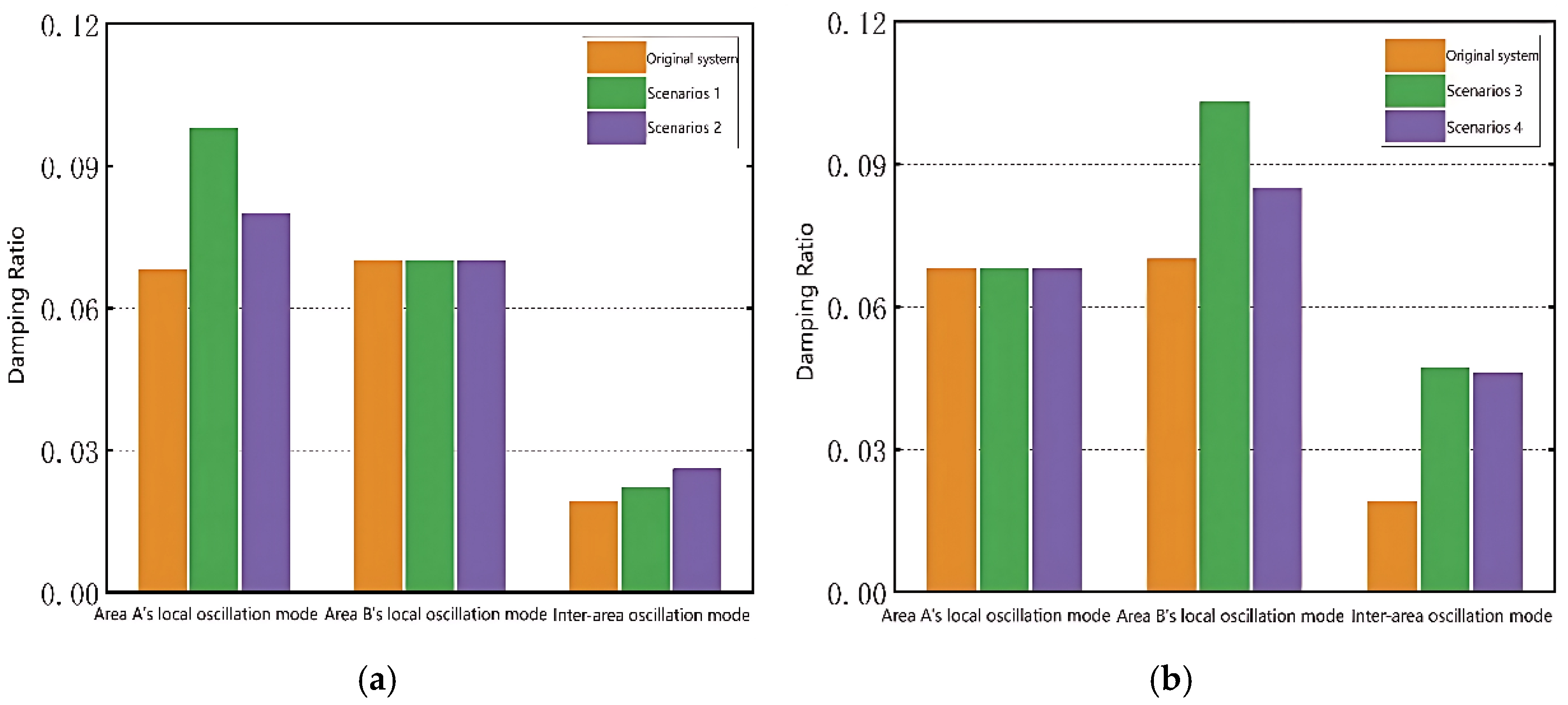
In all four scenarios, DFIG-VSPS integration improves both the local oscillation mode in the connected area and the inter-area oscillation mode to varying degrees, while showing no impact on local oscillation modes outside the connected area.

(3)

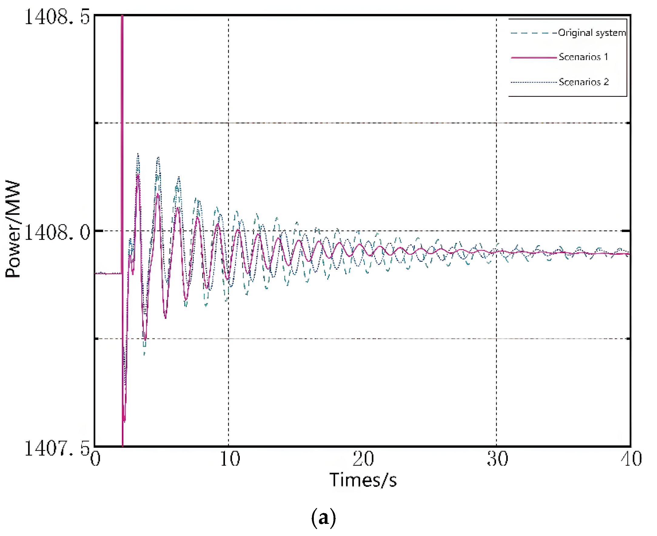
The improvement effect on regional oscillation modes is more pronounced when DFIG-VSPS is connected to the power-receiving area. The integration approach that maintains power balance by reducing synchronous generator output in the connected area proves more effective in enhancing the local oscillation mode of that area. Therefore, connecting DFIG-VSPS to the power-receiving area (Scenario 3) through synchronous generator output adjustment represents the optimal approach for improving system damping characteristics and strengthening the small signal stability of the interconnected system.

6.2.3. Simulation Verification

To validate the accuracy of the eigenvalue analysis results, time–domain simulations were conducted on the four-machine two-area system before and after DFIG-VSPS integration. A 5% step change was applied to the active load at L1 in Area A at 2 s, lasting for 0.1 s, to simulate small disturbances during system operation. The power responses of transmission lines between buses 6–7 and 9–10, as well as the tie-line power between Areas A and B, were used to characterize the local oscillation modes in each area and the inter-area oscillation mode. The simulation results of system power responses under various scenarios are shown in Figure 21.

An analysis of the three subplots in Figure 21 reveals that DFIG-VSPS integration improves the original oscillation modes in all cases, reducing the time required for power responses to stabilize after disturbances, though the degree of improvement varies. Subplot (b) demonstrates that connecting DFIG-VSPS to the power-receiving area produces significantly better improvement in inter-area oscillation modes compared with connection at the power-sending area. Comparative analysis of subplots (a) and (c) shows that the power balancing method involving synchronous generator output adjustment yields better improvement in local oscillation modes than the load addition approach. These time–domain simulation results align perfectly with the eigenvalue analysis conclusions presented in Section 6.2.2, thereby confirming the validity of the eigenvalue analysis method.

7. Conclusions

In this study, the speed control system of a water pump turbine, a doubly fed motor, and a converter and its control system were combined to develop a mathematical model of the DFIG-VSPS connected to a single-machine infinite bus system in the synchronous rotation $dq0$ coordinate system. The eigenvalue method was used to analyze the small-disturbance stability of the system for the first time. The results indicated that the unit had five pairs of OMs and six AMs. The primary factors that affect the OMs include the transient electromotive force d- and q-axis components, active output, DC voltage, grid-side current, and state variables related to the pump turbine speed control system of the DFIG. The AMs are affected by the reactive power and rotor-side current, and the state variables of the pump turbine speed control system also affect the AMs. Additionally, the analysis of the variation in the characteristic root trajectories showed that as the water flow inertia time constant T_w increased, the stability of the system weakened, posing a risk of instability.

In terms of control parameter optimization, properly adjusting the proportional parameter and integral parameter of the power outer loop controller can improve the system’s OM and enhance damping characteristics. However, it is necessary to consider the trade-off between dynamic performance and stability. For instance, increasing Kp can improve response speed but may lead to higher overshoot, while reducing Ki helps mitigate integral saturation but may degrade steady-state accuracy.

Therefore, in practical applications, the appropriate range for Kp and Ki should be determined through simulations or experiments based on specific operating conditions and stability requirements. This ensures a balanced compromise between dynamic response and stability margin.

However, this study only takes power generation conditions as an example and does not address the issue of small-disturbance stability under pumping conditions, and the eigenvalue method also has certain limitations. Therefore, in subsequent research, the small-disturbance stability of DFIG-VSPS and grid connected under pumping conditions should be considered, or another analysis method should be used to analyze the small-disturbance stability of DFIG-VSPS.

To provide a comprehensive understanding of DFIG-VSPS dynamics, future work will include the following: pumping condition analysis: extending the small-disturbance stability assessment to the pump operation mode, where different control strategies and hydraulic–mechanical dynamics may influence stability; and enhanced simulation validation: incorporating a wider range of operational scenarios (e.g., transition states, grid fault conditions) and comparative studies with other methods (e.g., eigenvalue sensitivity or time–domain simulations) to strengthen the robustness of the conclusions. These extensions will bridge the gap between theoretical analysis and practical implementation, ensuring the method’s applicability across all operational modes of DFIG-VSPS systems.

References

1. Papaefthymiou, S.V.; Lakiotis, V.G.; Margaris, I.D.; Papathanassiou, S.A. Dynamic analysis of island systems with wind-pumped-storage hybrid power stations. Renew. Energy 2015, 74, 544–554. [Google Scholar] [CrossRef]
2. Li, J.; Guo, W.; Liu, Y. Nonlinear state feedback-synergetic control for low frequency oscillation suppression in grid-connected pumped storage-wind power interconnection system. J. Energy Storage 2023, 73, 109281. [Google Scholar] [CrossRef]
3. Tan, X.; Li, C.; Liu, D.; Wang, H.; Xu, R.; Lu, X.; Zhu, Z. Multi-time scale model reduction strategy of variable-speed pumped storage unit grid-connected system for small-signal oscillation stability analysis. Renew. Energy 2023, 211, 985–1009. [Google Scholar] [CrossRef]
4. Mohanpurkar, M.; Ouroua, A.; Hovsapian, R.; Luo, Y.; Singh, M.; Muljadi, E.; Gevorgian, V.; Donalek, P. Real-time co-simulation of adjustable-speed pumped storage hydro for transient stability analysis. Electr. Power Syst. Res. 2018, 154, 276–286. [Google Scholar] [CrossRef]
5. Joseph, A.; Desingu, K.; Semwal, R.R.; Chilliah, T.R.; Khare, D. Dynamic performance of pumping mode of 250 MW variable speed hydro-generating unit subjected to power and control circuit faults. IEEE Trans. Energy Convers. 2018, 33, 430–441. [Google Scholar] [CrossRef]
6. Desingu, K.; Selvaraj, R.; Chelliah, T.R.; Khare, D. Effective utilization of parallel-connected megawatt three-level back-to-back power converters in variable speed pumped storage units. IEEE Trans. Ind. Appl. 2019, 55, 6414–6426. [Google Scholar] [CrossRef]
7. Lung, J.-K.; Lu, Y.; Hung, W.-L.; Kao, W.-S. Modeling and dynamic simulations of doubly fed adjustable-speed pumped storage units. IEEE Trans. Energy Convers. 2007, 22, 250–258. [Google Scholar] [CrossRef]
8. Gao, C.; Yu, X.; Nan, H.; Men, C.; Zhao, P.; Fu, J. A fast high-precision model of the doubly-fed pumped storage unit. J. Electr. Eng. Technol. 2021, 16, 797–808. [Google Scholar] [CrossRef]
9. Zhao, K.; Xu, Y.; Guo, P.; Qian, Z.; Zhang, Y.; Liu, W. Multi-scale oscillation characteristics and stability analysis of pumped-storage unit under primary frequency regulation condition with low water head grid-connected. Renew. Energy 2022, 189, 1102–1119. [Google Scholar] [CrossRef]
10. Li, S.; Xie, H.; Yan, Y.; Wu, T.; Huang, T.; Liu, Y.; Li, C.; Liang, H.; Cao, T. Excitation control of variable speed pumped storage unit for electromechanical transient modeling. Energy Rep. 2022, 8 (Suppl. 8), 818–825. [Google Scholar] [CrossRef]
11. Zhang, X.; Zhu, Z.; Fu, Y.; Li, L. Optimized virtual inertia of wind turbine for rotor angle stability in interconnected power systems. Electr. Power Syst. Res. 2020, 180, 106157. [Google Scholar] [CrossRef]
12. Gebru, F.M.; Khan, B.; Alhelou, H.H. Analyzing low voltage ride through capability of doubly fed induction generator based wind turbine. Comput. Electr. Eng. 2020, 86, 106727. [Google Scholar] [CrossRef]
13. Xu, H.; Li, Z.; Wu, H.; Zhao, R.; Hu, J. Reduced-order modeling of DFIG-based wind turbine connected into weak AC grid based on electromechanical time scale. Energy Rep. 2020, 6 (Suppl. 9), 886–895. [Google Scholar] [CrossRef]
14. Han, M.; Kawkabani, B.; Simond, J.-J. Eigenvalues analysis applied to the stability study of a variable speed pump turbine unit. In Proceedings of the 2012 XXth International Conference on Electrical Machines, Marseille, France, 2–5 September 2012; pp. 907–913. [Google Scholar] [CrossRef]
15. Wang, F.; Tan, T.; Liu, K.; Zhu, S.; Yang, J.; Li, Y.; Hu, C.; Qin, L. Small signal stability analysis of the joint operation system of variable speed pumped storage units and direct drive wind turbines. Electr. Power Autom. Equip. 2021, 41, 65–72. [Google Scholar] [CrossRef]
16. Gao, C.; Yu, X.; Nan, H.; Men, C.; Zhao, P.; Cai, Q.; Fu, J. Stability and dynamic analysis of doubly-fed variable speed pump turbine governing system based on Hopf bifurcation theory. Renew. Energy 2021, 175, 568–579. [Google Scholar] [CrossRef]
17. Guo, W.; Xu, X. Sliding mode control of regulating system of pumped storage power station considering nonlinear pump-turbine characteristics. J. Energy Storage 2022, 52, 105071. [Google Scholar] [CrossRef]
18. Shi, H.; Wang, Y.; Sun, X.; Chen, G.; Ding, L.; Pan, P.; Zeng, Q. Stability characteristics analysis and ultra-low frequency oscillation suppression strategy for FSC-VSPSU. Int. J. Electr. Power Energy Syst. 2024, 155, 109623. [Google Scholar] [CrossRef]
19. Si, Y.; Wang, Z.; Liu, L. Sensitivity analysis of power system small signal stability to geomagnetic disturbances. Int. J. Electr. Power Energy Syst. 2023, 148, 108970. [Google Scholar] [CrossRef]
20. de Toledo, P.F.; Bergdahl, B.; Asplund, G. Multiple infeed short circuit ratio—Aspects related to multiple HVDC into one AC network. In Proceedings of the 2005 IEEE/PES Transmission & Distribution Conference & Exposition: Asia and Pacific, Dalian, China, 18 August 2005; pp. 1–6. [Google Scholar] [CrossRef]
Figure 1. T-type equivalent circuit diagram of a doubly fed induction generator.
Energies 18 02796 g001
Figure 2. Control block diagram of pump turbine speed control system. P r e f refers to the reference power, ω o p t denotes the reference value for speed, h and q denote the head and flow obtained by the pump turbine, and y indicates the stroke of the servo system servomotor.
Energies 18 02796 g002
Figure 3. Control block diagram of the machine-side converter.
Energies 18 02796 g003
Figure 4. Control block diagram of the grid-side converter.
Energies 18 02796 g004
Figure 5. Structure diagram of the dual pulse width modulation converter.
Energies 18 02796 g005
Figure 6. Control strategy of doubly fed induction generator-based variable-speed pumped storage unit under a hydraulic turbine condition. Q s is generated by the direct connection between the stator windings and the power grid, calculated by the formula Q s = 3 2 V s I s sin s . V s represents stator voltage, I s denotes stator current, and s is the phase difference between them. Q g is produced through the interaction between the grid-side converter and the power grid, calculated by the formula Q g = 3 2 V g I g sin g . Here, V g stands for grid voltage, I g indicates grid-side converter output current, and g represents the phase difference.
Energies 18 02796 g006
Figure 7. Structure diagram of the unit connected to a single-machine infinite bus system.
Energies 18 02796 g007
Figure 8. Eigenvalue trajectory with increasing Tw. (a) OM4, (b) OM5, (c) AM1, (d) OM2.
Energies 18 02796 g008
Figure 9. Changes in damping ratio as Tw increases.
Energies 18 02796 g009
Figure 10. Characteristic root trajectory with increasing kp3.
Energies 18 02796 g010
Figure 11. Changes in damping ratio as kp3 increases.
Energies 18 02796 g011
Figure 12. Characteristic root trajectory with ki3 increasing.
Energies 18 02796 g012
Figure 13. Change in damping ratio with increasing ki3.
Energies 18 02796 g013
Figure 14. Unit speed response under different Tw.
Energies 18 02796 g014
Figure 15. Unit speed response at Tw = 2.8 s.
Energies 18 02796 g015
Figure 16. Unit power output response at different ki3 values. (a) ki3 = 10, (b) ki3 = 100.
Energies 18 02796 g016
Figure 17. Structure diagram of a DFIG-VSPS connected to the four-machine two-area system.
Energies 18 02796 g017
Figure 18. Eigenvalue distribution map of the four-machine two-area system.
Energies 18 02796 g018
Figure 19. Eigenvalue distribution map of the system under four scenarios. (a) Scenario 1, (b) Scenario 2, (c) Scenario 3, (d) Scenario 4.
Energies 18 02796 g019
Figure 20. The change in damping ratio in four scenarios. (a) Area A, (b) Area B.
Energies 18 02796 g020
Figure 21. Simulation results of system power response in each scenario. (a) Area A’s power response; (b) tie-line power response; (c) Area B’s power response.
Energies 18 02796 g021aEnergies 18 02796 g021b