Optimal Sliding Mode Control of Modular Multilevel Converters Considering Control Input Constraints

Abstract

This paper investigates the optimal sliding mode control (SMC) of modular multilevel converters (MMCs) by considering control input constraints. Conventional SMC methods for MMCs typically overlook the system’s constraints. To address this, an optimal SMC approach that incorporates control input constraints through quadratic programming (QP) is proposed. The control design problem is formulated in a constrained optimization framework and solved using the infeasible active-set (IAS) method to efficiently achieve the optimal solution. By applying optimal SMC, this work contributes to the advancement of SMC strategies for MMCs by addressing both constraints and performance optimization in a systematic way. This is particularly relevant for real-world applications, where controllers may temporarily exceed their limits before enforcing constraints. To validate the proposed approach, a comparative analysis with conventional SMC methods is performed, and simulation results confirm that the proposed approach provides improved performance.

1. Introduction

In recent years, modular multilevel converters (MMCs) have become a focus of interest, gaining prominence as leading converter solutions for medium- to high-voltage applications. The MMC offers several notable advantages, as highlighted in [1,2]: (i) a modular design allows scalability to various power and voltage levels; (ii) the capability to produce high-quality output voltages with more levels, minimizing filtering requirements; (iii) high efficiency; (iv) no need for the usual DC-bus capacitor, because the storage is allocated within the capacitors of the MMC’s submodules (SMs); and (v) a redundant configuration. Given these advantages, MMCs are particularly well-suited for grid-connected applications, including high-voltage direct-current (HVDC) transmission systems [3], static synchronous compensators (STATCOMs) [4], renewable energy conversion systems [5,6], battery energy storage systems (BESS) [7], etc.

Despite the numerous advantages of MMCs, controlling them remains complex and challenging. The main control objectives of an MMC typically involve regulating the AC-side phase currents to meet load requirements, as well as regulating circulating currents and submodule (SM) capacitor voltages [8]. The AC-side phase current control can be implemented in stationary $abc$ or $\alpha \beta$, and rotating $dq$ reference frames [9], with the aim of tracking the corresponding reference tailored to the type of application. The circulating current controller typically employs resonant controllers [10,11] to suppress even-order harmonics. Controlling submodule capacitor voltages usually involves two aspects: balancing the voltages of the SMs within each arm, which is indispensable for the stable operation of MMC, and regulating the total capacitor voltage of each phase leg (or energy of phase leg), which establishes the circulating current reference [10,12].

A range of classical controllers, such as proportional–integral (PI) and proportional–resonant (PR), alongside advanced techniques like model-predictive control (MPC) [13,14,15], as well as feedback linearization [8], have been developed in various research studies to meet MMC control objectives. Sliding mode control (SMC) has also been widely applied in the field of power electronics, offering key benefits such as robustness to uncertainties and disturbances, fast dynamic response, and simple implementation. Moreover, SMC does not require an exact system model [16,17]. However, SMC has some drawbacks, including chattering and the need for high gain [18]. Conventional SMC designs typically rely on worst-case scenarios, often resulting in an overestimation of the gain magnitude. This high gain, while effective for fast convergence and handling system uncertainties, leads to a significant issue in practical applications where constraints on the control input are common. Consequently, control input saturation occurs, causing performance degradation or even system instability [18].

In practical applications, the control inputs are constrained in magnitude, making it essential to account for this limitation during the design of SMC. Several studies have addressed the issue of keeping the control input within acceptable limits. Static adjustment methods impose predefined constraints on the control inputs to avoid exceeding their limits, while dynamic adjustment methods modify their behavior based on real-time conditions, offering more flexibility. For instance, the adaptive reaching law-based SMC method in [19,20] offers a solution to an overestimation of gain magnitude by dynamically adjusting the gain during the reaching phase, preventing excessive gain and, consequently, control inputs that could lead to saturation. Additionally, dynamic surface control (DSC) [21] has been employed as a dynamic adjustment technique that not only reduces chattering but also helps prevent control input saturation by ensuring control signals remain bounded. While adaptive-based methods offer flexibility, they present a challenge in fine-tuning and may introduce instability in systems with varying dynamics.

Several approaches employing SMC for the current control of MMCs have been presented in [17,22,23,24]. Despite their effectiveness, a key challenge with these conventional methods is that they overlook situations where control inputs exceed the actual physical limits of the MMC. This can lead to unrealistic control actions that degrade control system performance. It should be highlighted that in this case, the gains of the SMC laws play a crucial role in the control system’s performance. However, except for [17], where the lower bounds for the SMC parameters are determined through system dynamics analysis, other studies have disregarded this aspect.

To address such limitations in conventional SMC methods, it is essential to incorporate the physical limits of MMCs into the design of the control strategy. As will be presented in the following sections of this paper, the voltage applied to each arm of the MMC cannot exceed the sum of the submodule capacitor voltages. To address this challenge, this paper proposes an optimal SMC method that incorporates control input constraints, effectively accounting for the physical limits of the MMC. Initially, a proportional plus integral sliding surface is defined. Next, a performance index is formulated based on the dynamics of the sliding surface and the control inputs. This performance index is then transformed into a quadratic programming (QP) problem, where the control inputs serve as the optimization variables, allowing control input constraints to be directly integrated within the QP framework. Subsequently, the infeasible active-set (IAS) method from [25] is utilized to quickly determine the optimal solution for this control problem. This optimal solution (reference of arm voltages) can then be utilized in the modulation stage. The IAS method offers significant benefits for solving constrained optimization problems, primarily due to its simple structure and fast convergence. Additionally, the saturation solution is employed for comparison.

The key step in this paper involves determining the voltage references for the two arms of each phase based on a performance index that ensures the regulation of both AC-side phase currents and circulating currents. To accomplish this, we formulate a QP problem that incorporates the voltage bound of each arm as a constraint. The main contributions of this study are outlined as follows: (1) The constrained control problem is formulated within the SMC framework and transformed into a QP problem. (2) The IAS method is employed to efficiently solve the QP problem. This constrained optimization approach provides more accurate tracking performance compared to conventional methods, particularly under transient conditions.

The advantages of the approach presented in this paper can be summarized as follows. First, the control law is formulated within a constrained optimization space, ensuring systematic and reliable handling of the control input constraints. Second, in contrast to conventional SMC schemes in [23], this work utilizes an optimal solution, enabling improved control performance, particularly when the MMC operates under transient conditions.

The structure of the subsequent sections is as follows: Section 2 presents the mathematical model of the MMC and arm voltage bounds. Section 3.1 describes the formulation of the optimal SMC based on the MMC model, along with the representation of the MMC’s constraints. Then, the application of the IAS method to solve the QP problem is discussed in Section 3.2. Reference values for control variables are derived in Section 4.1, while Section 4.2 covers the inner-arm capacitor voltage balancing and modulation strategy. Section 5 provides the simulation results, and Section 6 summarizes the conclusion.

2. Mathematical Model of the MMC

The three-phase MMC is constructed by connecting N identical half-bridge submodules (HB-SMs) in series in each arm, as depicted in Figure 1. The MMC comprises three legs, each containing an upper ($u$) and lower ($l$) arm. Each submodule consists of a DC energy storage capacitor (C), two controllable semiconductor devices, and two anti-parallel diodes, forming a bidirectional HB-SM. Each SM can switch between insert and bypass states. In the insert state, the upper switch of the SM ($S_i$) conducts, and the SM voltage ($v_{{SM}_i}$) equals the SM capacitor voltage ($v_{c_i}$). In contrast, in the bypass state, the lower switch of SM (${\overline{S}}_i$) conducts, preventing current from circulating through the capacitor, resulting in zero SM voltage. Therefore, the voltage across the arbitrary i-th submodule, whether from the upper or lower arm of any arbitrary phase, can be expressed as follows:

$$v_{{SM}_i}=S_i v_{c_i}$$

(1)

where the $S_i$ is the switching state of the upper switch of submodule $i$, where $i$ is the submodule identifier, defined as follows:

$$S_i=\left\{\begin{array}{cc}1& insert state\\ 0& bypass state\end{array}\right.$$

(2)

Each arm includes an inductor (L) to mitigate arm current harmonics and limit fault currents. Furthermore, an equivalent arm resistor (R) is incorporated to model losses from various sources, including semiconductors, the equivalent series resistance of the SM capacitor, and the arm inductor, etc.

The DC-bus voltage, identified as $V_{dc}$, connects the $u$ and $l$ points, while $i_{dc}$ stands for the DC-bus current. The currents flowing through the upper and lower arms in three phases are labeled as $i_{u,a}$, $i_{l,a}$, $i_{u,b}$, $i_{l,b}$, $i_{u,c}$, and $i_{l,c}$. On the other hand, the voltages produced by the upper and lower arms in three phases are represented as $e_{u,a}$, $e_{l,a}$, $e_{u,b}$, $e_{l,b}$, $e_{u,c}$, and $e_{l,c}$. The MMC is connected to an ideal AC grid at the point of common coupling (PCC) through an AC filter, with the terminal AC voltages of the MMC being $v_{t,a}$, $v_{t,b}$, and $v_{t,c}$, while the three-phase grid voltages are $v_{g,a}$, $v_{g,b}$, and $v_{g,c}$.

The AC-side phase currents ($i_{s,j}$) for phase $j=a, b, c$, where $j$ is the phase identifier, can be achieved through:

$$i_{s,j}=i_{u,j}-i_{l,j}$$

(3)

The circulating currents ($i_{c,j}$) are defined as follows:

$$i_{c,j}={\displaystyle \frac{i_{u,j}+i_{l,j}}{2}}$$

(4)

Applying Kirchhoff’s Voltage Law (KVL) to the upper and lower arms of each phase, as shown in Figure 1, yields the equations for the upper and lower arm voltages with respect to the DC-bus virtual midpoint (O), as described in (5) and (6), respectively.

$$e_{u,j}={\displaystyle \frac{V_{dc}}{2}}-L{\displaystyle \frac{d{i}_{u,j}}{dt}}-R{i}_{u,j}-v_{t,j}$$

(5)

$$e_{l,j}={\displaystyle \frac{V_{dc}}{2}}-L{\displaystyle \frac{d{i}_{l,j}}{dt}}-R{i}_{l,j}+v_{t,j}$$

(6)

where $e_{u,j}$ and $e_{l,j}$ denote the upper and lower arm output voltages. Adding and subtracting (5) and (6), along with the integration of (3) and (4), yields a new set of equations as given in (7) and (8).

$${\displaystyle \frac{L}{2}}{\displaystyle \frac{d{i}_{s,j}}{dt}}=-{\displaystyle \frac{R}{2}}{i}_{s,j}-v_{t,j}+{\displaystyle \frac{{-e}_{u,j}+e_{l,j}}{2}}$$

(7)

$$L{\displaystyle \frac{d{i}_{c,j}}{dt}}=-R{i}_{c,j}+{\displaystyle \frac{V_{dc}-e_{u,j}-e_{l,j}}{2}}$$

(8)

Given that $v_{t,j}=R_g{i}_{s,j}+L_{g}d{i}_{s,j}/dt+v_{g,j}$, (7) can be reformulated as follows:

$$L_{eq}{\displaystyle \frac{d{i}_{s,j}}{dt}}=-R_{eq} i_{s,j}-v_{g,j}+{\displaystyle \frac{e_{l,j}-e_{u,j}}{2}}$$

(9)

where $R_g$ and $L_g$ are the resistance and inductance of the grid filter, $v_g$ represents grid voltage, $R_{eq}=R_g+R/2$, and $L_{eq}=L_g+L/2$.

Using (9) and (8), the dynamic behavior of AC-side phase currents and circulating currents can be described as follows:

$${\displaystyle \frac{d{i}_{s,j}}{dt}}={\displaystyle \frac{1}{L_{eq}}}\left(-R_{eq} i_{s,j}-v_{g,j}+{\displaystyle \frac{e_{l,j}-e_{u,j}}{2}}\right)$$

(10)

$${\displaystyle \frac{d{i}_{c,j}}{dt}}={\displaystyle \frac{1}{L}}\left(-R{i}_{c,j}+{\displaystyle \frac{V_{dc}}{2}}-{\displaystyle \frac{e_{l,j}+e_{u,j}}{2}}\right)$$

(11)

Since the arm voltages $e_{u,j}$ and $e_{l,j}$ are the sum of the output voltages of the SMs, we have:

$$e_{u,j}=\sum _{i=1}^N{v}_{{SM}_{i,j}}=\sum _{i=1}^N{S}_{u_{i,j}}{v}_{{cu}_{i,j}}$$

(12)

$$e_{l,j}=\sum _{i=N+1}^{2N}{v}_{{SM}_{i,j}}=\sum _{i=N+1}^{2N}{S}_{l_{i,j}}{v}_{{cl}_{i,j}}$$

(13)

where $S_{u_{i,j}}$ and $S_{l_{i,j}}$ represent the insertion states of each SM in the upper and lower arms of phase $j$, respectively. $v_{{cu}_{i,j}}$ and $v_{{cl}_{i,j}}$ represent the capacitor voltages of the i-th SM of the upper and lower arms, respectively. According to (12) and (13), the maximum value of the arm voltage is the sum of all the SM capacitor voltages in the respective arm, which can be simplified to (14) and (15).

$$0\le e_{u,j}\le \sum _{i=1}^N{v}_{{cu}_{i,j}}$$

(14)

$$0\le e_{l,j}\le \sum _{i=N+1}^{2N}{v}_{{cl}_{i,j}}$$

(15)

The primary control variables crucial for an MMC are the AC-side phase currents and the circulating currents. Thus, according to (10) and (11), by choosing the state vector $x\in {\mathbb{R}}^6={[i_{s,j}^T i_{c,j}^T]}^T$, output vector $y\in {\mathbb{R}}^6={[i_{s,j}^T i_{c,j}^T]}^T$ and input vector $u\in {\mathbb{R}}^6={[e_{u,j}^T e_{l,j}^T]}^T$, the state-space model can be described as follows:

$$\left\{\begin{array}{l}{\dot{x}}_{(6\times 1)}=A_{(6\times 6)}{x}_{(6\times 1)}+B_{(6\times 6)}{u}_{(6\times 1)}+d_{(6\times 1)}\\ y_{(6\times 1)}=C_{(6\times 6)}{x}_{(6\times 1)}\end{array}\right.$$

(16)

where:

$$\begin{gathered} i_{s,j}=\left[\begin{array}{c}{i}_{s,a}\\ i_{s,b}\\ i_{s,c}\end{array}\right], i_{c,j}=\left[\begin{array}{c}{i}_{c,a}\\ i_{c,b}\\ i_{c,c}\end{array}\right], e_{u,j}=\left[\begin{array}{c}{e}_{u,a}\\ e_{u,b}\\ e_{u,c}\end{array}\right], e_{l,j}=\left[\begin{array}{c}{e}_{l,a}\\ e_{l,b}\\ e_{l,c}\end{array}\right], v_{g,j}=\left[\begin{array}{c}{v}_{g,a}\\ v_{g,b}\\ v_{g,c}\end{array}\right], v_{dc}=\left[\begin{array}{c}{V}_{dc}\\ V_{dc}\\ V_{dc}\end{array}\right], \\ A={\left[\begin{array}{cc}diag\left(-{\displaystyle \frac{R_{eq}}{L_{eq}}}\right)& 0_{3\times 3}\\ 0_{3\times 3}& diag\left(-{\displaystyle \frac{R}{L}}\right)\end{array}\right]}_{6\times 6},B={\left[\begin{array}{cc}\begin{array}{c}diag\left({\displaystyle \frac{-1}{{2L}_{eq}}}\right)\end{array}& \begin{array}{c}diag\left({\displaystyle \frac{+1}{{2L}_{eq}}}\right)\end{array}\\ diag\left({\displaystyle \frac{-1}{2L}}\right)& diag\left({\displaystyle \frac{-1}{2L}}\right)\end{array}\right]}_{6\times 6}, \\ d\in {\mathbb{R}}^6={\left[\begin{array}{cc}-{\displaystyle \frac{v_{g,j}^T}{L_{eq}}}& {\displaystyle \frac{v_{dc}^T}{2L}}\end{array}\right]}^T. \end{gathered}$$

Since there are multiple inputs, the constraints are specified for each input individually.

It is important to note that this paper adopts the arm voltages as the control input vector, following the approach outlined in [26], while the selection of insertion indices can be performed as described in [27].

3. Formulation of Optimal Sliding Mode Control for MMCs

3.1. Performance Index and Optimization Problem Formulation

The first step in the design process of sliding mode control is to define a stable sliding surface. To ensure a fair comparison with the proposed method in [23], the PI form of the sliding surface is considered as follows:

$$S(t)=\epsilon (t)+\lambda {\int }_0^t\epsilon \left(t\right) dt$$

(17)

where $\epsilon \left(t\right)=y^{*}\left(t\right)-y\left(t\right)$ represents the tracking error and $y^{*}={\left[\begin{array}{cc}{i_{s,j}^{*}}^T& {i_{c,j}^{*}}^T\end{array}\right]}^T$ is the desired output. Furthermore, $\lambda$ represents a diagonal matrix with constant and positive parameters on the diagonal, defined as follows:

$$\lambda =\left[\begin{array}{cc}{\lambda }_{s,j}& 0_{3\times 3}\\ 0_{3\times 3}& {\lambda }_{c,j}\end{array}\right],{\lambda }_{s,j}=\left[\begin{array}{ccc}{\lambda }_{s,a}& 0& 0\\ 0& {\lambda }_{s,b}& 0\\ 0& 0& {\lambda }_{s,c}\end{array}\right], {\lambda }_{c,j}=\left[\begin{array}{ccc}{\lambda }_{c,a}& 0& 0\\ 0& {\lambda }_{c,b}& 0\\ 0& 0& {\lambda }_{c,c}\end{array}\right].$$

(18)

where, under the assumption of a symmetrical system, ${\lambda }_{s,a}={\lambda }_{s,b}={\lambda }_{s,c}={\lambda }_s$, and ${\lambda }_{c,a}={\lambda }_{c,b}={\lambda }_{c,c}={\lambda }_c$. The vector of the sliding surface is represented as follows:

$$S=\left[\begin{array}{c}{S}_{s,j}\\ \\ S_{c,j}\end{array}\right], S_{s,j}=\left[\begin{array}{c}{S}_{s,a}\\ S_{s,b}\\ S_{s,c}\end{array}\right],S_{c,j}=\left[\begin{array}{c}{S}_{c,a}\\ S_{c,b}\\ S_{c,c}\end{array}\right].$$

(19)

The next step concerns the design strategy of the optimal SMC law using the proposed PI sliding surface. To establish the optimal SMC law for the MMC system, the following performance index is introduced, extending the approach from [18], which originally addressed single-input single-output (SISO) systems. Thus, the performance index is defined for the multi-input multi-output (MIMO) model of the MMC system as follows:

$$J={\displaystyle \frac{1}{2}}{\left(\dot{S}+\alpha S\right)}^T\beta (\dot{S}+\alpha S)+{\displaystyle \frac{1}{2}}{u}^T\gamma u$$

(20)

The performance index includes matrix weighting factors as $\alpha \in {\mathbb{R}}^{6\times 6}, \beta \in {\mathbb{R}}^{6\times 6}$ and $\gamma \in {\mathbb{R}}^{6\times 6}$ with positive diagonal elements, where:

$$\begin{gathered} \alpha =\left[\begin{array}{cc}{\alpha }_{s,j}& 0_{3\times 3}\\ 0_{3\times 3}& {\alpha }_{c,j}\end{array}\right],{\alpha }_{s,j}=\left[\begin{array}{ccc}{\alpha }_{s,a}& 0& 0\\ 0& {\alpha }_{s,b}& 0\\ 0& 0& {\alpha }_{s,c}\end{array}\right],{\alpha }_{c,j}=\left[\begin{array}{ccc}{\alpha }_{c,a}& 0& 0\\ 0& {\alpha }_{c,b}& 0\\ 0& 0& {\alpha }_{c,c}\end{array}\right], \\ \beta =\left[\begin{array}{cc}{\beta }_{s,j}& 0_{3\times 3}\\ 0_{3\times 3}& {\beta }_{c,j}\end{array}\right],{\beta }_{s,j}=\left[\begin{array}{ccc}{\beta }_{s,a}& 0& 0\\ 0& {\beta }_{s,b}& 0\\ 0& 0& {\beta }_{s,c}\end{array}\right],{\beta }_{c,j}=\left[\begin{array}{ccc}{\beta }_{c,a}& 0& 0\\ 0& {\beta }_{c,b}& 0\\ 0& 0& {\beta }_{c,c}\end{array}\right], \\ \gamma =\left[\begin{array}{cc}{\gamma }_{s,j}& 0_{3\times 3}\\ 0_{3\times 3}& {\gamma }_{c,j}\end{array}\right],{\gamma }_{s,j}=\left[\begin{array}{ccc}{\gamma }_{s,a}& 0& 0\\ 0& {\gamma }_{s,b}& 0\\ 0& 0& {\gamma }_{s,c}\end{array}\right],{\gamma }_{c,j}=\left[\begin{array}{ccc}{\gamma }_{c,a}& 0& 0\\ 0& {\gamma }_{c,b}& 0\\ 0& 0& {\gamma }_{c,c}\end{array}\right]. \end{gathered}$$

where, under the assumption of a symmetrical system, it can be assumed that ${\alpha }_{s,a}={\alpha }_{s,b}={\alpha }_{s,c}={\alpha }_s$, ${\alpha }_{c,a}={\alpha }_{c,b}={\alpha }_{c,c}={\alpha }_c$, ${\beta }_{s,a}={\beta }_{s,b}={\beta }_{s,c}={\beta }_s$, ${\beta }_{c,a}={\beta }_{c,b}={\beta }_{c,c}={\beta }_c$, ${\gamma }_{s,a}={\gamma }_{s,b}={\gamma }_{s,c}={\gamma }_s$, and ${\gamma }_{c,a}={\gamma }_{c,b}={\gamma }_{c,c}={\gamma }_c$.

The first term of the performance index contains the square of the first-order dynamics of the sliding surface. Consequently, minimizing (20) corresponds to the convergence of this dynamics to zero. On the other hand, the second term of (20) concerns the minimization of control effort. Minimizing the performance index in (20) leads to an optimal control law where a trade-off is achieved between the minimum tracking error and the minimum control effort [18].

The derivative of the sliding surface, as defined in (17), is given by:

$$\dot{S}=\dot{\epsilon }+\lambda \epsilon$$

(21)

By using (16), the derivative of the error can be calculated as follows:

$$\dot{\epsilon }={\dot{y}}^{*}-\dot{y}={\dot{y}}^{*}-C\dot{x}={\dot{y}}^{*}-CAx-CBu-Cd$$

(22)

Substituting (22) into (21) gives:

$$\dot{S}={\dot{y}}^{*}-CAx-CBu-Cd+\lambda (y^{*}-y)$$

(23)

Then, substituting (23) into (20) transforms (20) into (24).

$$J={\displaystyle \frac{1}{2}}{\left[{\dot{y}}^{*}-CAx-CBu-Cd+\lambda \left(y^{*}-Cx\right)+\alpha S\right]}^T \beta \left[{\dot{y}}^{*}-CAx-CBu-Cd+\lambda (y^{*}-Cx)+\alpha S\right]+{\displaystyle \frac{1}{2}}{u}^T\gamma u$$

(24)

This equation can be rewritten, considering the control inputs as the optimization variables. By expanding and disregarding the term that does not rely on the control inputs, (24) can be transformed into a QP problem, as below:

$$J_{new}={\displaystyle \frac{1}{2}}{u}^T{\left(CB\right)}^T\beta \left(CB\right)u+{\displaystyle \frac{1}{2}}{u}^T\gamma u-{\displaystyle \frac{1}{2}}{\mathsf{\Psi }}^T\beta \left(CB\right)u-{\displaystyle \frac{1}{2}}{u}^T{\left(CB\right)}^T\beta \mathsf{\Psi }$$

(25)

where $\mathsf{\Psi }$ is the intermediate vector, defined as,

$$\mathsf{\Psi }={\dot{y}}^{*}-CAx-Cd+\lambda (y^{*}-Cx)+\alpha S$$

By reorganizing the terms in (25), it can be expressed as a QP problem as follows:

$$J_{QP}={\displaystyle \frac{1}{2}}{u}^T\left[{\left(CB\right)}^T\beta \left(CB\right)+\gamma \right]u-{\displaystyle \frac{1}{2}}{\mathsf{\Psi }}^T\beta \left(CB\right)u-{\displaystyle \frac{1}{2}}{u}^T{\left(CB\right)}^T\beta \mathsf{\Psi }$$

(26)

Subsequently, (26) can be restructured into a QP problem in the following manner:

$$J_{QP}={\displaystyle \frac{1}{2}}{u}^{T}Hu+u^{T}F$$

(27a)

where:

$$H={\left(CB\right)}^T\beta \left(CB\right)+\gamma$$

(27b)

$$F=-{\left(CB\right)}^T\beta \mathsf{\Psi }.$$

(27c)

where H and F are the coefficient matrices of the quadratic function.

By substituting from (16) and (20) into (27b), H can be obtained as:

$$H\in {\mathbb{R}}^{6\times 6}=\left[\begin{array}{cc}\left({\displaystyle \frac{1}{4L_{eq}^2}}\right){\beta }_{s,j}+\left({\displaystyle \frac{1}{4L^2}}\right){\beta }_{c,j}+{\gamma }_{s,j}& \left({\displaystyle \frac{-1}{4L_{eq}^2}}\right){\beta }_{s,j}+\left({\displaystyle \frac{1}{4L^2}}\right){\beta }_{c,j}\\ \left({\displaystyle \frac{-1}{4L_{eq}^2}}\right){\beta }_{s,j}+\left({\displaystyle \frac{1}{4L^2}}\right){\beta }_{c,j}& \left({\displaystyle \frac{1}{4L_{eq}^2}}\right){\beta }_{s,j}+\left({\displaystyle \frac{1}{4L^2}}\right){\beta }_{c,j}+{\gamma }_{c,j}\end{array}\right]$$

(28)

The matrix H is symmetric and can be rewritten as:

$$\left[\begin{array}{cc}\underset{H_1}{\underbrace{\left({\displaystyle \frac{{\beta }_s}{4L_{eq}^2}}+{\displaystyle \frac{{\beta }_c}{4L^2}}+{\gamma }_s\right)I_3}}& \underset{H_2}{\underbrace{\left({\displaystyle \frac{-{\beta }_s}{4L_{eq}^2}}+{\displaystyle \frac{{\beta }_c}{4L^2}}\right)I_3}}\\ \underset{H_3}{\underbrace{\left({\displaystyle \frac{-{\beta }_s}{4L_{eq}^2}}+{\displaystyle \frac{{\beta }_c}{4L^2}}\right)I_3}}& \underset{H_4}{\underbrace{\left({\displaystyle \frac{{\beta }_s}{4L_{eq}^2}}+{\displaystyle \frac{{\beta }_c}{4L^2}}+{\gamma }_c\right)I_3}}\end{array}\right]$$

(29)

where $I_3$ is a $3\times 3$ identity matrix. Since H is a block matrix and $H_1$ is invertible, H is positive definite if and only if [28]:

$$H_1>0, S=H_4-H_3{H}_1^{-1}{H}_2>0$$

(30)

Since all leading principal minors of $H_1$ and S are positive, H is positive definite. Thus, (27a) is strictly convex [29].

By substituting from (16), (20), and (25) into (27c), we obtain $F$ as:

$$F\in {\mathbb{R}}^{6\times 1}=\left[\begin{array}{c}\left({\displaystyle \frac{d{i}_{s,j}^{*}}{dt}}+{\displaystyle \frac{R_{eq}}{L_{eq}}}{i}_{s,j}+{\displaystyle \frac{v_{g,j}}{L_{eq}}}+{\lambda }_{s,j}\left(i_{s,j}^{*}-i_{s,j}\right)+{\alpha }_{s,j}{S}_{s,j}\right){\displaystyle \frac{{\beta }_{s,j}}{2L_{eq}}}+\\ \left({\displaystyle \frac{d{i}_{c,j}^{*}}{dt}}+{\displaystyle \frac{R}{L}}{i}_{c,j}-{\displaystyle \frac{v_{dc}}{2L}}+{\lambda }_{c,j}\left(i_{c,j}^{*}-i_{c,j}\right)+{\alpha }_{c,j}{S}_{c,j}\right){\displaystyle \frac{{\beta }_{c,j}}{2L}}\\ \left({\displaystyle \frac{d{i}_{s,j}^{*}}{dt}}+{\displaystyle \frac{R_{eq}}{L_{eq}}}{i}_{s,j}+{\displaystyle \frac{v_{g,j}}{L_{eq}}}+{\lambda }_{s,j}\left(i_{s,j}^{*}-i_{s,j}\right)+{\alpha }_{s,j}{S}_{s,j}\right){\displaystyle \frac{-{\beta }_{s,j}}{2L_{eq}}}+\\ \left({\displaystyle \frac{d{i}_{c,j}^{*}}{dt}}+{\displaystyle \frac{R}{L}}{i}_{c,j}-{\displaystyle \frac{v_{dc}}{2L}}+{\lambda }_{c,j}\left(i_{c,j}^{*}-i_{c,j}\right)+{\alpha }_{c,j}{S}_{c,j}\right){\displaystyle \frac{{\beta }_{c,j}}{2L}}\end{array}\right]$$

(31)

Given the constraints on the control inputs within a closed convex space, where $u_{lb}\le u\le u_{ub}$, and the vectors $u_{lb}$ and $u_{ub}$ representing the lower and upper bounds of the control inputs, respectively, the constrained standard QP problem about $u={[e_{u,a} e_{u,b} e_{u,c} e_{l,a} e_{l,b} e_{l,c}]}^T$ can be expressed as:

$$\begin{array}{c}\mathit{min}\hspace{1em}{\displaystyle \frac{1}{2}}{u}^{T}Hu+u^{T}F\\ s.t.\hspace{1em}{u}_{lb}\le u\le u_{ub}\end{array}$$

(32)

In order to relate the constraints to the QP problem, the next step is to determine the lower and upper bounds of the constraints, represented by $0\le e_{u,j}\le e_{u,j}^{max}$ and $0\le e_{l,j}\le e_{l,j}^{max}$, in the following form.

$$\begin{array}{c}{u}_{lb}={\left[\begin{array}{cccccc}0& 0& 0& 0& 0& 0\end{array}\right]}^T,\\ u_{ub}={\left[\begin{array}{cc}{e}_{u,j}^{max}& e_{l,j}^{max}\end{array}\right]}^T,\end{array}$$

(33a)

where, according to (14) and (15):

$$e_{u,j}^{max}=\sum _{i=1}^N{v}_{{cu}_{i,j}}, e_{l,j}^{max}=\sum _{i=N+1}^{2N}{v}_{{cl}_{i,j}}.$$

(33b)

Since the cost function $J_{QP}$ is quadratic with the constraints as in (33), determining the optimal sliding mode control transforms into solving a standard QP problem, where the problem to be optimized is as follows:

$$\begin{array}{c}\begin{array}{c}min\\ u\end{array}{J}_{QP}\left(u\right)\\ s.t. u_{lb}\le u\le u_{ub}\end{array}$$

(34)

3.2. Solving QP Problem for Arm Voltage References Determination Using the Infeasible Active-Set Method

By taking the derivative with respect to u, the global solution of the unconstrained form of (32) can be derived as:

$${\nabla }_u J_{QP}\left(u\right)=Hu+F=0$$

(35)

This leads to the unconstrained solution expressed as:

$$u_{unc}=-H^{-1}F$$

(36)

However, if the solution obtained from (36) does not meet the constraints specified in (33), a typical saturation solution [27] can be applied as:

$$u_{sat}=min(u_{ub},\mathit{max}\left(u_{lb},u_{unc}\right))$$

(37)

Numerous techniques are available for solving QP problems while considering the constraints. Active-set and interior-point methods [29,30], which typically require multiple iterative steps, are widely recognized as effective strategies for addressing QP problems.

To address the optimization problem while considering constraints, the Lagrangian function for (32) can be expressed as:

$$\mathcal{L}\left(u,p,q\right)={\displaystyle \frac{1}{2}}{u}^{T}Hu+u^{T}F+p^T\left(u-u_{ub}\right)+q^T\left(u_{lb}-u\right)$$

(38)

where $p\in {\mathbb{R}}^6$ and $q\in {\mathbb{R}}^6$ are vectors of Lagrange multipliers associated with the upper and lower bound constraints, respectively. The vector $u\in {\mathbb{R}}^6$, along with vectors $p$ and $q$, represents the solution to problem (32) if ($u,p,q$) satisfies the following Karush–Kuhn–Tucker (KKT) conditions [25,27]:

$$Hu+F+p-q=0$$

(39a)

$$p_k\left(u_k-u_{ub}\right)=0, \forall k\in \mathcal{N}$$

(39b)

$$q_k\left(u_{lb}-u_k\right)=0, \forall k\in \mathcal{N}$$

(39c)

$$u_{lb}\le u\le u_{ub}, p\ge 0, q\ge 0.$$

(39d)

where $\mathcal{N}=\left\{1, 2, \dots , n\right\}$ is the set of positive integers, with $n$ representing the dimension of $u$. The solution process is iterative. At each step, the first-order optimality condition from (39a) and the complementarity constraints from (39b) and (39c) are satisfied. The iterations continue until the feasibility of ($u,p,q$) is achieved, as specified in (39d).

Active-set methods iteratively solve the problem, considering only the equality constraints in the current active set, terminating once the optimal active set is found. In this paper, we employ the infeasible active-set method [25] to solve the quadratic programming problem, as detailed in Algorithm 1. The IAS method, known for its fast convergence, efficiently solves quadratic programming problems in just a few iterations regardless of assumptions. The proof of the IAS algorithm’s convergence is presented in [25], demonstrating that the algorithm converges in a finite number of steps.

A key step in solving (39) is identifying the active inequalities. Some working sets, namely ${\mathsf{A}}_l$, ${\mathsf{A}}_u$, and $I$, are predefined. The set ${\mathsf{A}}_l$ contains indices where the lower bound constraint is active, meaning that for each $k\in {\mathsf{A}}_l$, $u_k$ reaches the lower bound, i.e., $u_k=u_{lb}=0$. Similarly, ${\mathsf{A}}_u$ represents the indices where the upper bound constraint is active, with $u_k=u_{ub}$ for each $k\in {\mathsf{A}}_u$. The overall active constraint set $A$ is the union of ${\mathsf{A}}_l$ and ${\mathsf{A}}_u$, i.e., $\mathsf{A}={\mathsf{A}}_l\bigcup {\mathsf{A}}_u$. The complementary set $I$ is defined as $I=\mathcal{N}\setminus \mathsf{A}$, where for each $k\in I$, $u_k$ lies strictly between the lower and upper bounds. Based on the current working sets ${\mathsf{A}}_l$, ${\mathsf{A}}_u$, and $I$, along with the complementarity conditions in (39b) and (39c), the following equations can be readily derived.

$$u_{{\mathsf{A}}_l}=0, p_{{\mathsf{A}}_l}=0,$$

(40a)

$$u_{{\mathsf{A}}_u}=u_{ub}, q_{{\mathsf{A}}_u}=0,$$

(40b)

$$p_I=0, q_I=0.$$

(40c)

These conditions arise because an active bound constraint forces its corresponding Lagrange multiplier to be zero. It is important to note that we denote $u_{{\mathsf{A}}_l}$ as the components of $u$ corresponding to the indices in ${\mathsf{A}}_l$, i.e., $u_{{\mathsf{A}}_l}≔{\left(u_k\right)}_{k\in {\mathsf{A}}_l}$, and this notation applies similarly to other sets. The remaining elements $u_I$, $p_{{\mathsf{A}}_u}$, and $q_{{\mathsf{A}}_l}$ need to be determined. To do so, we utilize (39a) and separate the equations and variables based on ${\mathsf{A}}_u$, ${\mathsf{A}}_l$, and $I$ as follows:

$$\left[\begin{array}{ccc}{H}_{{\mathsf{A}}_u{\mathsf{A}}_u}& H_{{\mathsf{A}}_u{\mathsf{A}}_l}& H_{{\mathsf{A}}_{u}I}\\ H_{{\mathsf{A}}_l{\mathsf{A}}_u}& H_{{\mathsf{A}}_l{\mathsf{A}}_l}& H_{{\mathsf{A}}_{l}I}\\ H_{I{\mathsf{A}}_u}& H_{I{\mathsf{A}}_l}& H_{II}\end{array}\right]\left[\begin{array}{c}{u}_{{\mathsf{A}}_u}\\ u_{{\mathsf{A}}_l}\\ u_I\end{array}\right]+\left[\begin{array}{c}{F}_{{\mathsf{A}}_u}\\ F_{{\mathsf{A}}_l}\\ F_I\end{array}\right]+\left[\begin{array}{c}{p}_{{\mathsf{A}}_u}\\ p_{{\mathsf{A}}_l}\\ p_I\end{array}\right]-\left[\begin{array}{c}{q}_{{\mathsf{A}}_u}\\ q_{{\mathsf{A}}_l}\\ q_I\end{array}\right]=0$$

(41)

where for example $H_{{\mathsf{A}}_u{\mathsf{A}}_l}$ denotes the submatrix of H, defined as $H_{{\mathsf{A}}_u{\mathsf{A}}_l}={\left(h_{km}\right)}_{k\in A_u, m\in A_l}$. The third set of equations can be solved for $u_I$ as:

$$u_I=-H_{II}^{-1}(F_I+H_{I{\mathsf{A}}_u}{u}_{{\mathsf{A}}_u}+H_{I{\mathsf{A}}_l}{u}_{{\mathsf{A}}_l})$$

(42)

As $H_{II}$ is positive definite, it ensures that system (42) is solvable. Then, $p_{{\mathsf{A}}_u}$ and $q_{{\mathsf{A}}_l}$ can be determined as follows:

$$p_{{\mathsf{A}}_u}=-H_{{\mathsf{A}}_u{\mathsf{A}}_u}{u}_{{\mathsf{A}}_u}-H_{{\mathsf{A}}_u{\mathsf{A}}_l}{u}_{{\mathsf{A}}_l}-H_{{\mathsf{A}}_{u}I}{u}_I-F_{{\mathsf{A}}_u}$$

(43)

$$q_{{\mathsf{A}}_l}=H_{{\mathsf{A}}_l{\mathsf{A}}_u}{u}_{{\mathsf{A}}_u}+H_{{\mathsf{A}}_l{\mathsf{A}}_l}{u}_{{\mathsf{A}}_l}+H_{{\mathsf{A}}_{l}I}{u}_I+F_{{\mathsf{A}}_l}$$

(44)

If the current active set $\mathsf{A}$ is correctly identified, the conditions $0\le u_I\le u_{ub}$, $p_{{\mathsf{A}}_u}\ge 0$, and $q_{{\mathsf{A}}_l}\ge 0$ will be satisfied. If the current guess is incorrect, a new guess for the working sets ${\mathsf{A}}_l$, ${\mathsf{A}}_u$, and $\mathsf{A}$ must be made for the next iteration, denoted as ${\mathsf{A}}_l^{+}$, ${\mathsf{A}}_u^{+}$, and ${\mathsf{A}}^{+}$.

By considering $p_{{\mathsf{A}}_u}$, if $p_{{\mathsf{A}}_u}>0$ for $k\in {\mathsf{A}}_u$, this validates our previous guess that $k\in {\mathsf{A}}_u$, and index $k$ should be incorporated into the updated working set ${\mathsf{A}}_u^{+}$. The same condition applies for $q_{{\mathsf{A}}_l}$; if $q_k>0$ for $k\in {\mathsf{A}}_l$, index $k$ should similarly be incorporated into the updated working set ${\mathsf{A}}_l^{+}$. Considering $u_I$, when $u_k>u_{ub}$, $u_k$ is set to $u_{ub}$ in the next iteration, and $k$ is also added to ${\mathsf{A}}_u^{+}$ in this case. Similarly, when $u_k<0$, $u_k=0$ in the next iteration, and $k$ is included in ${\mathsf{A}}_l^{+}$. Thus, the update for new working sets can be presented as follows:

$${\mathsf{A}}_l^{+}:=\left\{k : u_k<0 or u_k=0 \& q_k>0\right\},$$

(45a)

$$A_u^{+}:=\left\{k : u_k>u_{ub} or u_k=u_{ub} \& p_k>0\right\},$$

(45b)

$$\mathsf{A}={\mathsf{A}}_l^{+}\cup A_u^{+}.$$

(45c)

With these updated working sets, the process can be repeated to obtain a new solution and check whether the KKT conditions are satisfied.

Algorithm 1: Infeasible active-set method [25,27]

Input: $[i_{s,j},i_{s,j}^{*},d{i}_{s,j}^{*}/dt,S_{s,j},i_{c,j},i_{c,j}^{*},d{i}_{c,j}^{*}/dt,S_{c,j}, v_{g,j},v_{dc},u_{ub},u_{lb},\alpha ,\beta ,\gamma ,\lambda ]$

1: Compute H and F according to (29) and (31).

2: $\mathcal{N}\leftarrow \left\{1, 2, \dots , n\right\}$; ${\mathsf{A}}_u\leftarrow \varnothing$; ${\mathsf{A}}_l\leftarrow \varnothing$; $I\leftarrow \mathcal{N}\backslash {\mathsf{A}}_u\backslash {\mathsf{A}}_l$;

3: Flag $\leftarrow$ 0;

4: while Flag == 0 do

5:   $u_{{\mathsf{A}}_u}\leftarrow u_{ub}$; $u_{{\mathsf{A}}_l}\leftarrow u_{lb}$;

6:   $p_{{I\cup \mathsf{A}}_l}\leftarrow 0$; $q_{{I\cup \mathsf{A}}_u}\leftarrow 0$;

7:   Compute $u_I$, $p_{{\mathsf{A}}_u}$ and $q_{{\mathsf{A}}_l}$ from (42), (43) and (44).

8:   if $u_{lb}\le u\le u_{ub} \& p\ge 0 \& q\ge 0$

9:    $u_{opt}=u$;

10:   Flag $\leftarrow$ 1;

11:  end if

12: ${\mathsf{A}}_u={\mathsf{A}}_u^{+}\leftarrow \left\{k : u_k>u_{ub} \parallel p_k>0\right\}$;

13: ${\mathsf{A}}_l={\mathsf{A}}_l^{+}\leftarrow \left\{k : u_k<0 \parallel q_k>0\right\}$;

14: $I\leftarrow \mathcal{N}\backslash {\mathsf{A}}_u\backslash {\mathsf{A}}_l$;

15: end while

Output: $u_{opt}=u={[e_{u,a}^{*} e_{u,b}^{*} e_{u,c}^{*} e_{l,a}^{*} e_{l,b}^{*} e_{u,c}^{*}]}^T$

The optimal solution $u_{opt}={[e_{u,a}^{*} e_{u,b}^{*} e_{u,c}^{*} e_{l,a}^{*} e_{l,b}^{*} e_{u,c}^{*}]}^T$, which defines the arm voltage references, is obtained after applying the infeasible active-set method. This solution can be utilized in the modulation stage.

Since the arm voltage is selected as the control input, the matrix H is constant, as shown in (29). As the inverse of H needs to be calculated for solving the QP problem, it can be precomputed offline and stored, which significantly reduces the computational load [27]. Moreover, since the problem has a small scale with only six dimensions, the optimization can be solved efficiently within a single control cycle, making it suitable for real-time implementation.

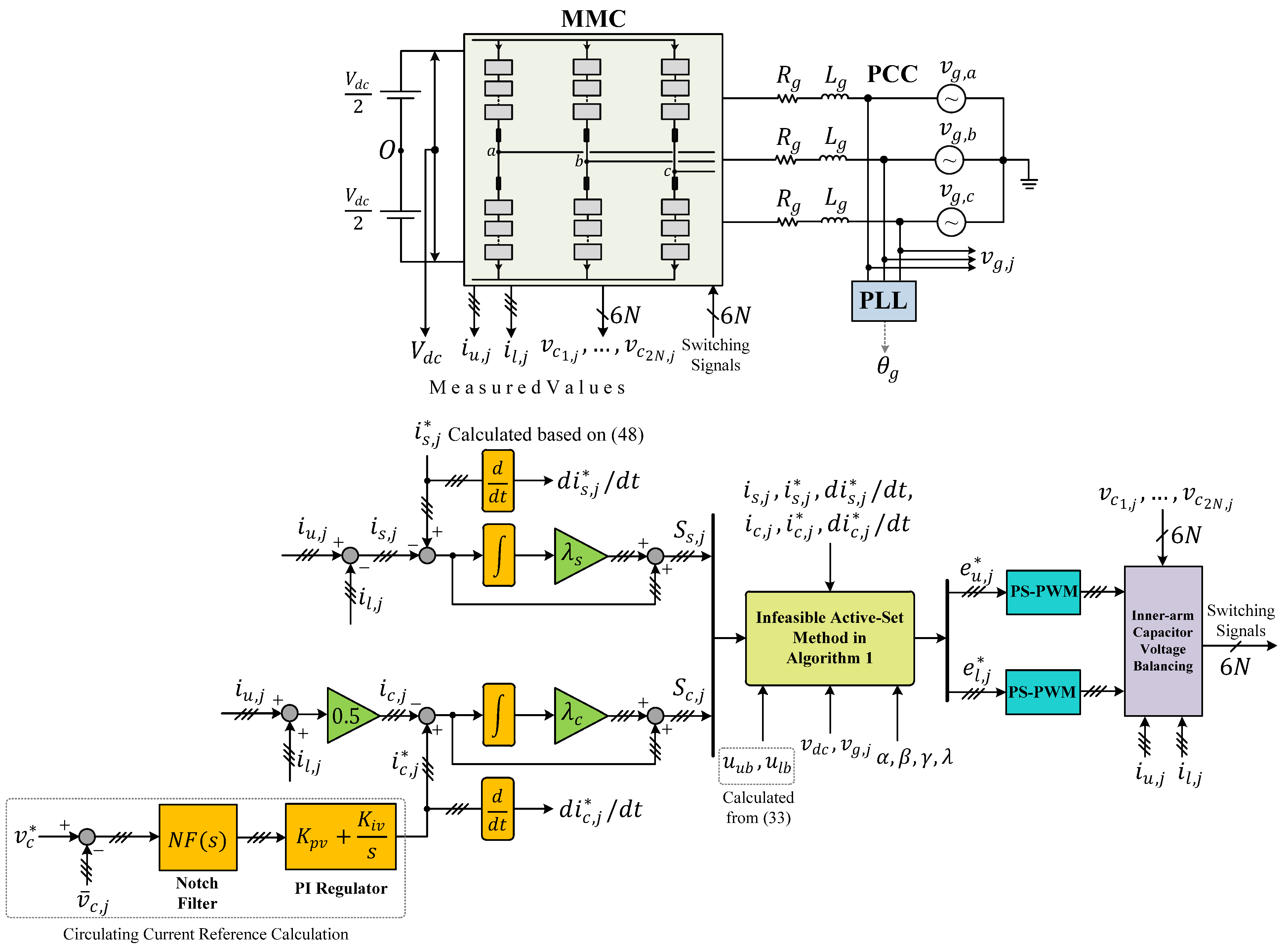
4. Reference Calculation and Low-Level Control Strategy

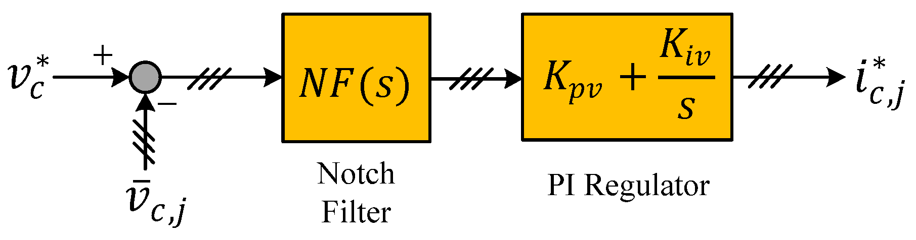
4.1. Reference Values

In the context of circulating current control, achieving the reference values requires employing an external leg-level balancing method. This method ensures that the average of 2N submodule capacitor voltages in each leg (${\overline{v}}_{c,j}$) as given in (46) remains constant at a specified value $v_c^{*}$ (which is the submodule capacitor reference voltage) [10,12]. In other words, this method stabilizes the operation of MMC by evenly distributing the voltage among the three-phase legs and generating the value for the circulating current reference.

$${\overline{v}}_{c,j}=0.5\left({\displaystyle \frac{1}{N}} \sum _{i=1}^N{v}_{ci,j}+{\displaystyle \frac{1}{N}}\sum _{i=N+1}^{2N}{v}_{ci,j}\right)$$

(46)

As stated by [8,31], second-order oscillations are present in ${\overline{v}}_{c,j}$. Such voltage oscillations bring additional disturbances to the reference of circulating currents. Consequently, the voltage oscillations are eliminated from the voltage control loops through the application of the notch filter (NF) depicted in Figure 2, where its transfer function is as follows:

$$NF(s)={\displaystyle \frac{s^2+{{\omega }_n}^2}{s^2+2\zeta {\omega }_{n}s+{{\omega }_n}^2}}$$

(47)

where the center angular frequency of the notch filter is denoted as ${\omega }_n=2{\omega }_0$, and the fundamental angular frequency is ${\omega }_0=2\pi f_0=120\pi$. The sharpness of the notch filter is determined by $2\zeta {\omega }_n$, where $\zeta$ represents the damping ratio of the filter. The $\zeta$ is designated as 0.1. This damping ratio is related to the filter’s quality factor $Q$, where $Q=1/2\zeta$.

In Figure 2, $K_{pv}$ and $K_{iv}$ are the leg-level balancing proportional and integral gains, respectively.

Moreover, given the grid voltage amplitude $V_g$ and the desired power ($P^{*}$), the steady-state references for the AC-side phase currents of the MMC can be determined as follows:

$$i_{s,j}^{*}=\left[\begin{array}{c}{i}_{s,a}^{*}\\ i_{s,b}^{*}\\ i_{s,c}^{*}\end{array}\right]=\left[\begin{array}{c}{I}_s^{*} sin\left({\theta }_g\right)\\ I_s^{*} sin({\theta }_g-2\pi /3)\\ I_s^{*} sin({\theta }_g+2\pi /3)\end{array}\right]$$

(48)

where ${\theta }_g$ is the grid voltage angle synchronized with phase $a$, which is determined by measuring the grid voltage and then extracted using a phase-locked loop (PLL). $I_s^{*}=2P^{*}/3V_g$ represents the amplitude of the desired AC-side phase currents.

4.2. Modulation and Inner-Arm Capacitor Voltage Balancing Strategy

The control layers of each MMC, organized in a cascaded control structure, can be divided into high-level and low-level controls [32]. In this paper, low-level control includes the implementation of phase-shifted PWM (PS-PWM) and the slow-rate inner-arm capacitor voltage balancing. Once the optimal arm voltage references have been determined by high-level control using optimal SMC, the PS-PWM block as described in [33] is used to select the optimal insertion index (the number of SMs to be inserted) for both arms of each phase. After that, switching signals for each SM are generated by employing a slow-rate inner-arm capacitor voltage balancing strategy aimed at balancing the capacitor voltages of the SMs in each arm, as outlined in [34]. This strategy ensures that the sorting algorithm operates at a low execution frequency, thereby leading to a significant reduction in the switching frequency of the MMC [35]. The PS-PWM is applied by comparing the upper and lower arm voltage references ($e_{u,j}^{*}$ and $e_{l,j}^{*}$) with N triangular carriers, each shifted by ${360}^{°}/N$ in each arm and with a carrier frequency of $f_c$. No phase shift is required between the triangular carriers of the upper and lower arms, resulting in the terminal voltage of the MMC consisting of N+1 distinct voltage levels.

According to the explanations provided up to this point, the overall control block diagram of the proposed optimal sliding mode control incorporating control input constraints is illustrated in Figure 3.

5. Simulation Results and Discussion

To assess the performance and effectiveness of the proposed control strategy, a three-phase MMC connected to a stiff grid was simulated in the MATLAB/Simulink environment, using the system parameters provided in

Table 1. System parameters.

Parameters	Value	Unit
Grid Parameters
Rated line-to-line RMS grid voltage	4160	V
Grid fundamental frequency ($f_0$)	60	Hz
Grid filter inductance ($L_g$)	8	mH
MMC Parameters
Rated power	1	MVA
DC-bus voltage ($V_{dc}$)	7	kV
Arm inductance (L)	5	mH
Equivalent arm resistance (R)	0.1	Ω
Number of submodules per arm (N)	8	---
Submodule capacitance (C)	8	mF
SM capacitor nominal voltage ($v_{cn}=V_{dc}/N$)	875	V
Control Parameters
Fundamental sample time	2	$\mathsf{\mu }\mathrm{s}$
Carrier frequency ($f_c$)	500	Hz
Leg-level balancing proportional gain ($K_{pv}$)	3.8	A·V−1
Leg-level balancing integral gain ($K_{iv}$)	30	A·V−1·s−1

. A discrete fixed-step solver with a fundamental sampling time of 2 $\mathsf{\mu }\mathrm{s}$ is used. The two control layers are executed at larger time steps. In this section, we present the simulation results of the conventional SMC methods from [23] with and without control input constraint, in comparison with the optimal SMC methods that include constraints. We refer to the optimal SMC with control input constraints that incorporate saturated control input as in (37), saturated optimal SMC (Sat-OSMC). The method where the optimal solution is obtained using the infeasible active-set method is termed as constrained optimal SMC (Cons-OSMC).

To evaluate the effectiveness of the proposed optimal SMC methods, we carried out a comparison with the conventional SMC methods outlined in [23]. For differentiation, we label the method with a simple proportional sliding surface as SMC-PI and the one with an integral sliding surface as ISMC-PI, as they use SMC and integral SMC methods for AC-side current control and a PI-based second-order harmonic suppression controller for circulating current control. It is worth mentioning that these conventional methods do not account for the constraints on the control inputs. We also consider modified versions of these methods that include control input saturation constraints as in (37). These are referred to as Sat-SMC-PI and Sat-ISMC-PI, respectively.

The parameters for the constant plus proportional rate reaching law, i.e., $Q_{d,q} sgn\left(S_{d,q}\right)+K_{d,q} S_{d,q}$, in both the SMC-PI and ISMC-PI methods and their modified versions are set as $K_d=K_q=600$, $Q_d=Q_q=1$. For the ISMC-PI and Sat-ISMC-PI methods, the sliding surface parameters are selected as ${\lambda }_d={\lambda }_q=0.4$. The PI-based circulating current controller parameters are chosen as $K_{pd}=K_{pq}=2.5$ and $K_{id}=K_{iq}=50$. The weighting factors used in the performance index of the proposed method are selected as ${\alpha }_s=200$, ${\alpha }_c=10$, ${\beta }_s=200$, ${\beta }_c=10$, ${\gamma }_s={\gamma }_c=200$. In addition, the sliding surface parameters are ${\lambda }_s=500, {\lambda }_c=8\times {10}^3$. In this work, we determined these weighting factors and parameters through a trial and error process until achieving the desired control performance. Moreover, as discussed in the introduction, one challenge with SMC designs is the reliance on overestimated gain magnitudes, typically chosen to handle worst-case scenarios. While this high gain can result in fast convergence and effective handling of uncertainties, it can lead to control input saturation in practice. The parameter selection process in this work is such that, as will be shown later, the control input values before applying the constraints were nearly the same across all methods, indicating that the parameters were overestimated for the given operating point change.

Offline simulation tests are carried out and presented in this paper. While this paper focuses on offline results, the proposed control method has been designed with real-time implementation feasibility in consideration. As mentioned earlier in this paper, the inverse of constant matrix H can be precomputed and stored offline, along with the low switching frequency achieved through the slow-rate inner-arm capacitor voltage balancing strategy, which allows for an efficient reduction in the computational load of the proposed control strategy. It should be noted that, in grid-connected MMCs, a low switching frequency can be advantageous, as it effectively reduces switching losses without compromising the system’s performance. As a result, real-time simulations are expected to yield results comparable to the offline simulations presented here. A full real-time implementation will be pursued in future work to further validate the proposed method’s applicability.

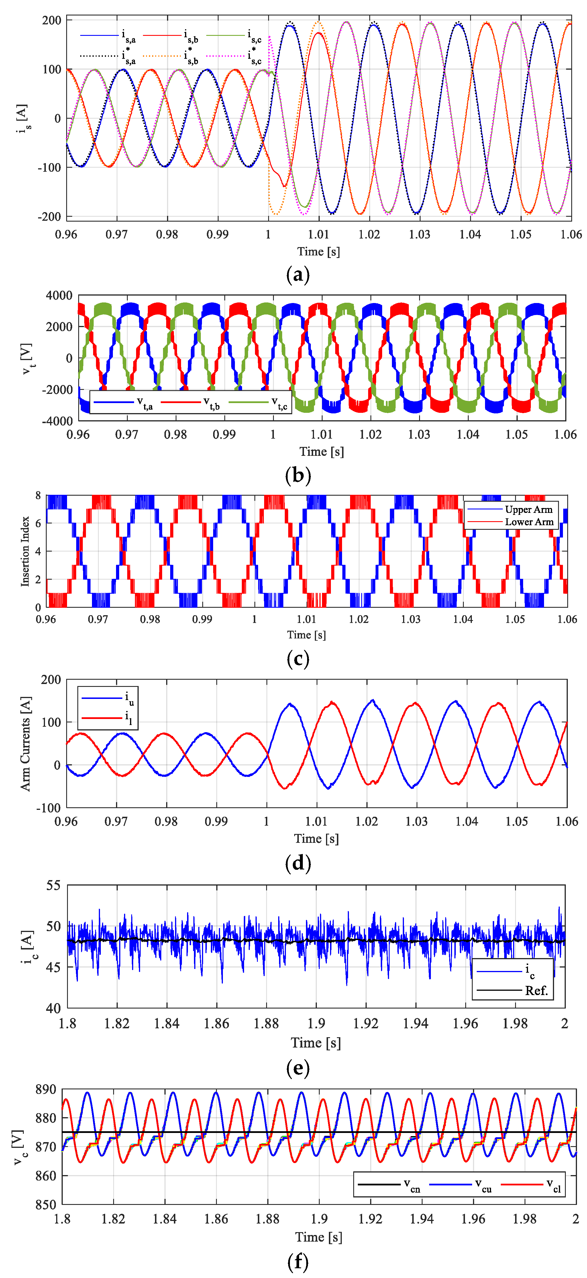
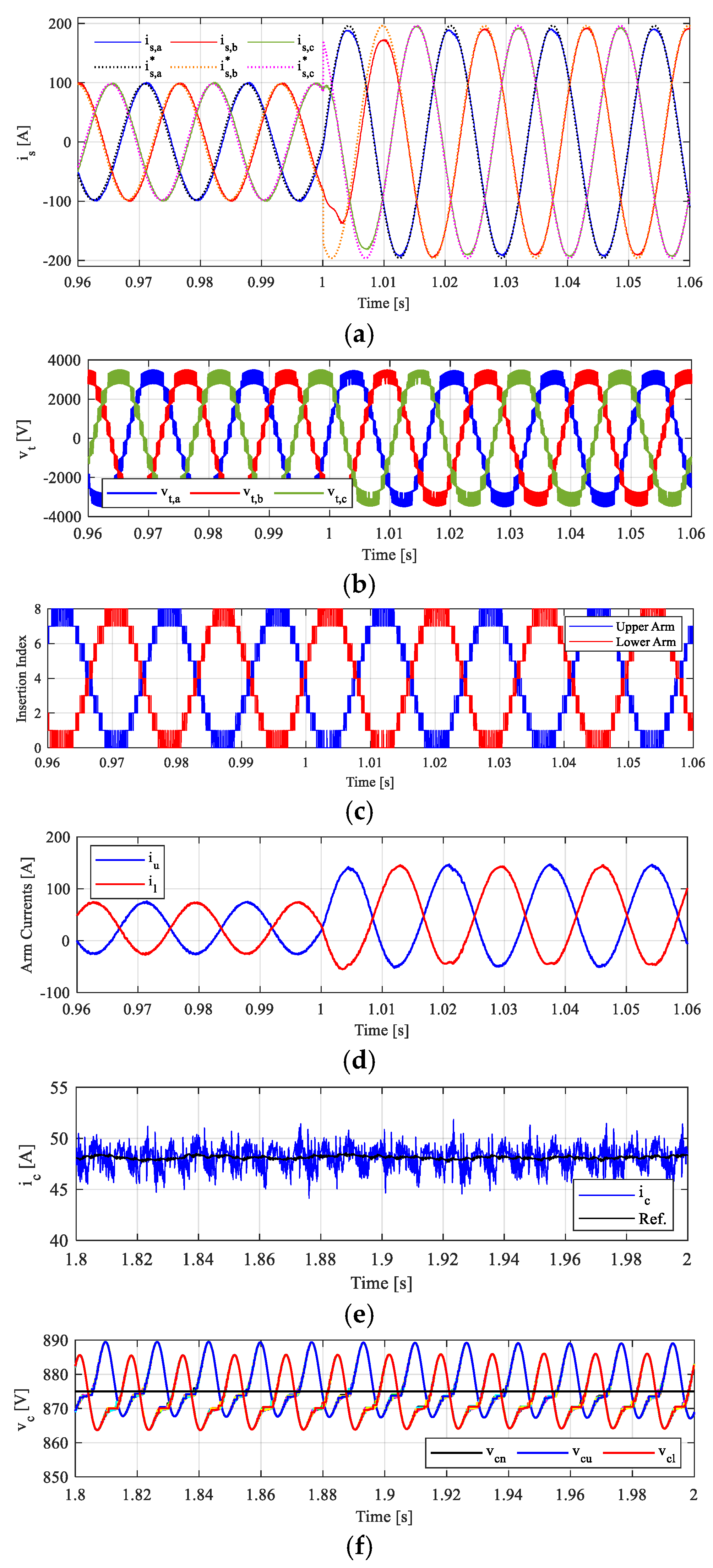
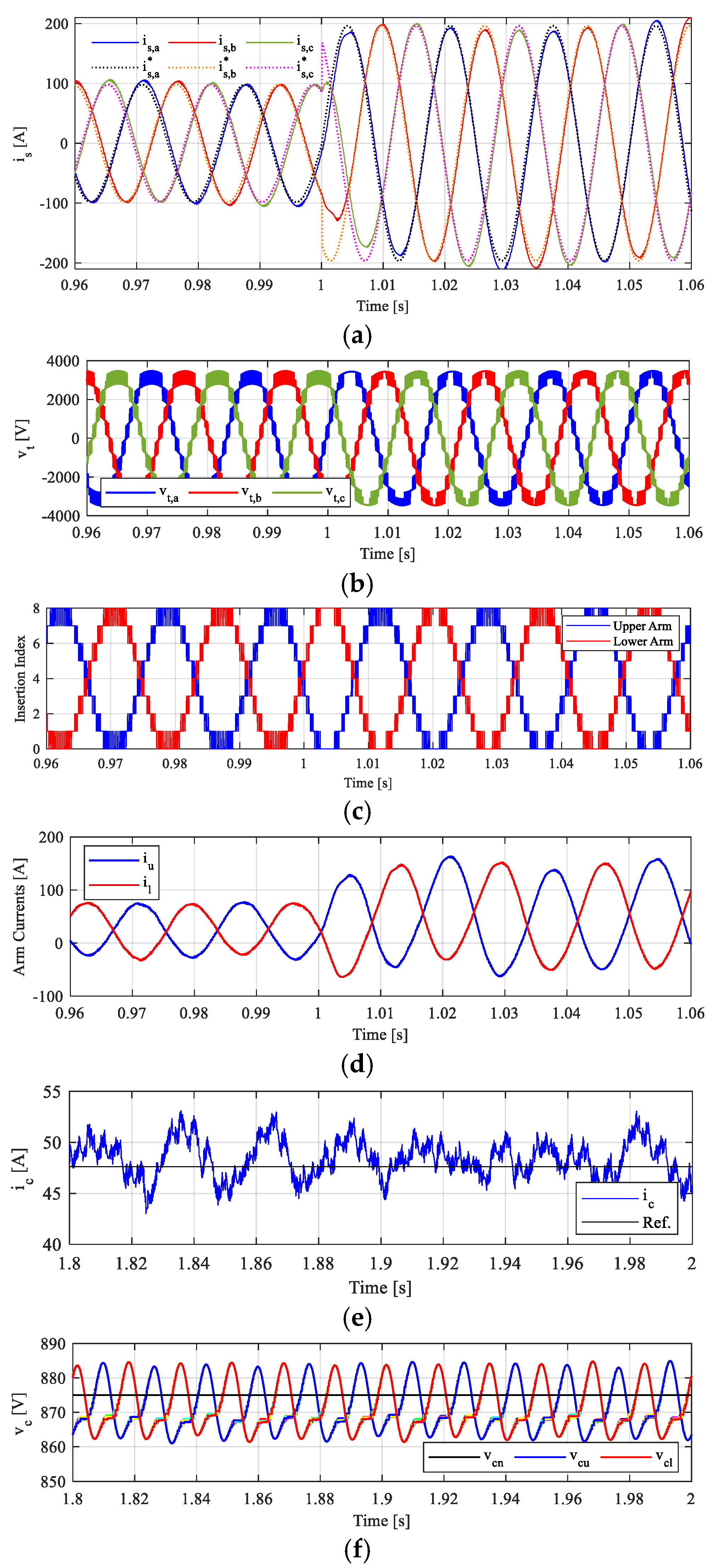
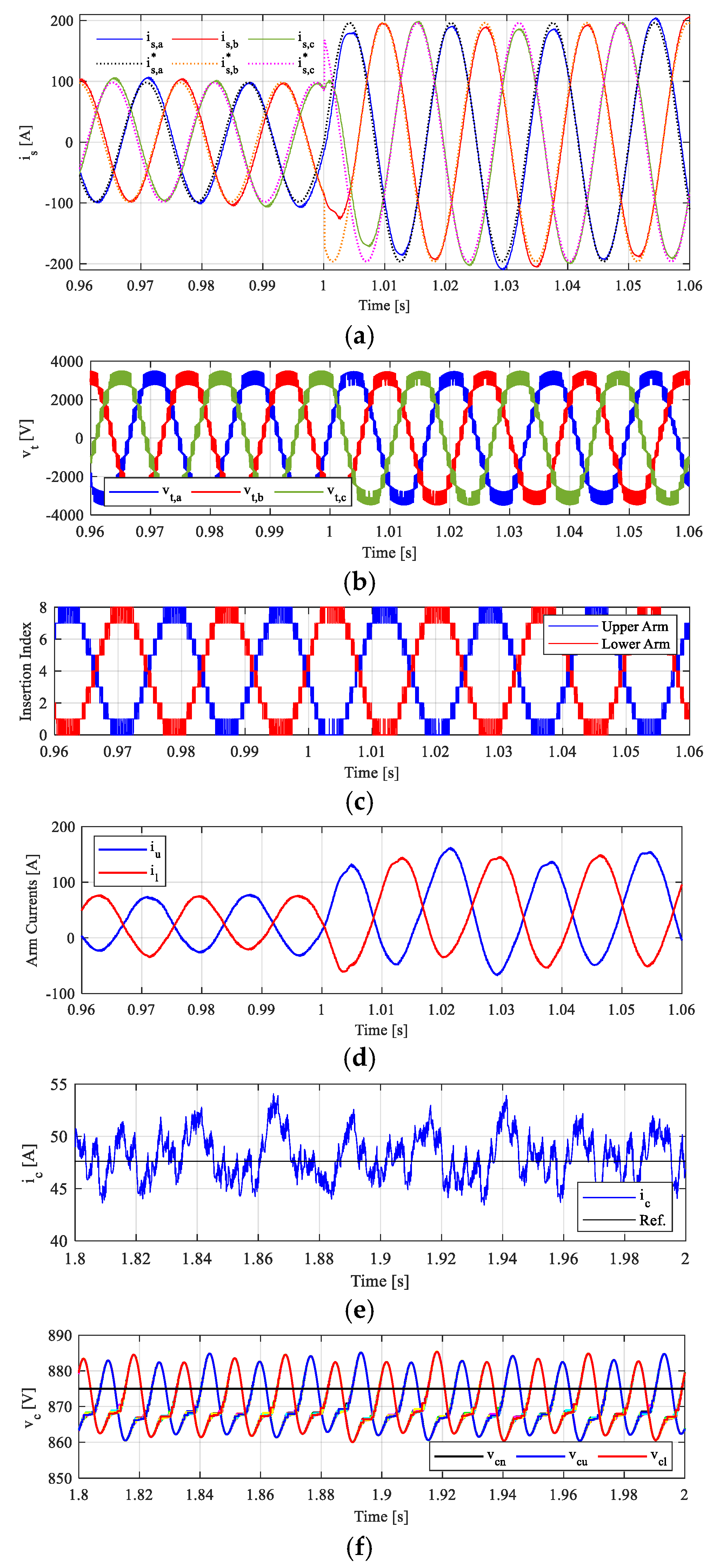
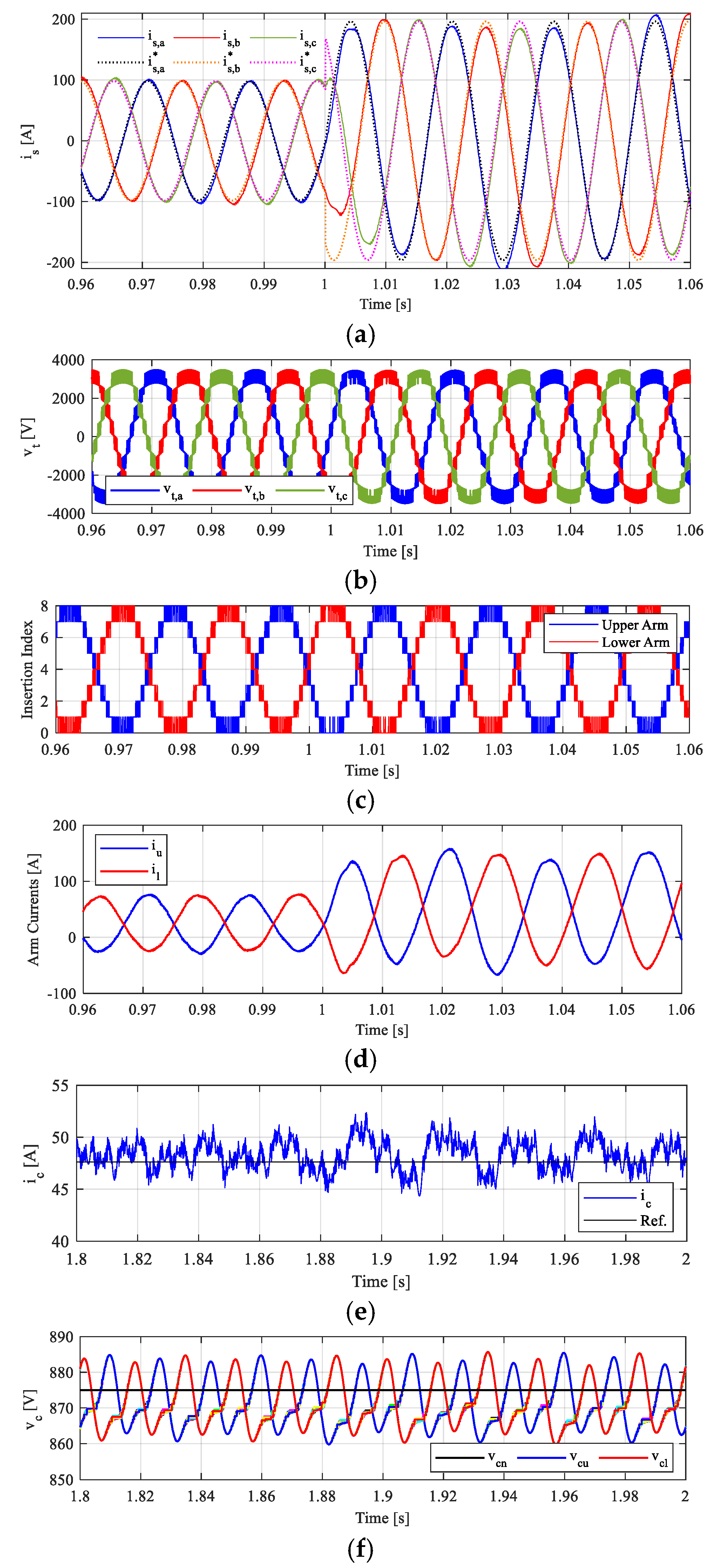
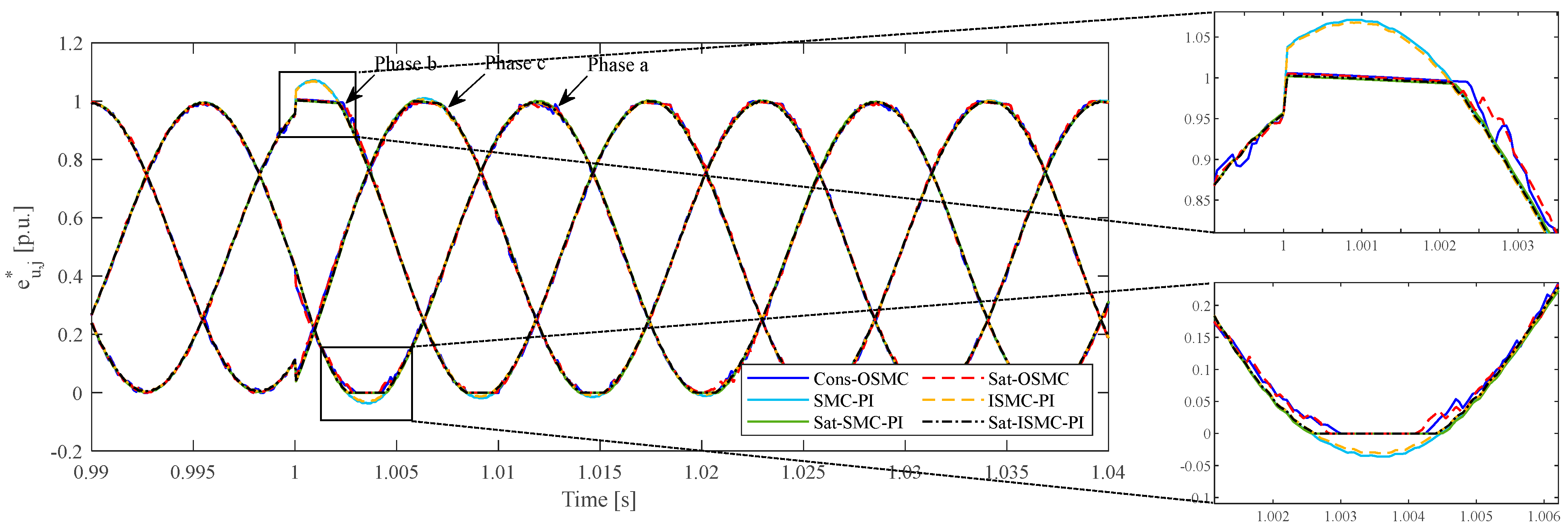
Dynamic and Steady-State Performance Under Transient Due to AC-Side Power Change

This section examines the performance of the MMC in response to a step change in AC-side active power. Initially, the MMC operates at $P^{*}=500 \mathrm{k}\mathrm{W}$ and $Q^{*}=0 \mathrm{V}\mathrm{A}\mathrm{R}$, with the desired AC-side current amplitude reference at $I_s^{*}=98.1 \mathrm{A}$. At t = 1 s, the request for AC-side active power is increased to $P^{*}=1 \mathrm{M}\mathrm{W}$, resulting in a new value of the AC-side current reference at $I_s^{*}=196.3 \mathrm{A}$.

Figure 4a, Figure 5a, Figure 6a, Figure 7a, Figure 8a and Figure 9a display the three-phase AC-side currents ($i_{s,a}$, $i_{s,b}$, and $i_{s,c}$) along with their reference under a related change. Across all methods, the current tracking for $i_{s,a}$, $i_{s,b}$, and $i_{s,c}$ exhibits a satisfactory dynamic response, with the currents adjusting to reference changes. Figure 4b, Figure 5b, Figure 6b, Figure 7b, Figure 8b and Figure 9b show terminal voltage waveforms, illustrating N + 1 = 9 distinct voltage levels. It is evident that the MMC system maintains stability under an operating point step change in all cases.

Figure 4c, Figure 5c, Figure 6c, Figure 7c, Figure 8c and Figure 9c show the insertion indices for both the upper and lower arms in phase a. It is clear that the selection of the insertion index combinations has less flexibility in both the SMC-PI and ISMC-PI methods during transients, compared to OSMC-based methods. Essentially, the SMC-PI and ISMC-PI methods have fewer choices in how they select insertion indices during rapid change. Consequently, the dynamic performance of the SMC-PI and ISMC-PI methods is affected by this limitation.

Figure 4d, Figure 5d, Figure 6d, Figure 7d, Figure 8d and Figure 9d and Figure 4e, Figure 5e, Figure 6e, Figure 7e, Figure 8e and Figure 9e show the upper and lower arm currents and the circulating current in steady-state, respectively. The steady-state upper and lower arm capacitor voltages, along with the nominal capacitor voltage $v_{cn}$ (indicated by the black line), are presented in Figure 4f, Figure 5f, Figure 6f, Figure 7f, Figure 8f and Figure 9f. The results indicate that the submodule capacitor voltages are consistently balanced in both arms in all cases.

The performance indices used to evaluate the effectiveness of each control method include the integral of absolute error (IAE) of the AC-side current ($i_s$) during both transient and steady-state, and the total harmonic distortion (THD) of the circulating current ($i_c$) in steady-state.

Table 2. Performance indices for all methods.

	Cons-OSMC	Sat-OSMC	SMC-PI	ISMC-PI	Sat-SMC-PI	Sat-ISMC-PI
IAE of $i_s$ in transient	Phase a: 0.29	Phase a: 0.31	Phase a: 0.77	Phase a: 0.80	Phase a: 0.69	Phase a: 0.77
	Phase b: 0.64	Phase b: 0.68	Phase b: 0.85	Phase b: 0.96	Phase b: 0.81	Phase b: 0.91
	Phase c: 0.36	Phase c: 0.39	Phase c: 0.86	Phase c: 0.91	Phase c: 0.78	Phase c: 0.85
IAE of $i_s$ in steady-state	Phase a: 2.04	Phase a: 2.06	Phase a: 3.15	Phase a: 2.99	Phase a: 3.76	Phase a: 2.79
	Phase b: 2.04	Phase b: 2.02	Phase b: 3.04	Phase b: 3.01	Phase b: 3.45	Phase b: 2.67
	Phase c: 1.98	Phase c: 2.00	Phase c: 3.22	Phase c: 2.95	Phase c: 3.90	Phase c: 2.74
THD of $i_c$ in steady-state	4.27%	3.03%	5.00%	4.32%	6.45%	4.25%

summarizes the results across all six control strategies. Transient duration is considered as the first 100 ms after a step change in reference. Lower values in these indices indicate better control performance, where a lower IAE represents more accurate tracking and lower THD reflecting reduced harmonic distortion and improved current quality.

The OSMC-based methods achieve the lowest IAE in transient across all phases, showing superior dynamic performance in tracking the reference of AC-side phase currents. Specifically, Cons-OSMC reduces transient error by 48% compared to SMC-PI, 52% compared to ISMC-PI, 43% compared to Sat-SMC-PI, and 49% compared to Sat-ISMC-PI. The Sat-OSMC also shows strong performance, with an average IAE only 7% higher than Cons-OSMC. These results demonstrate that the OSMC-based controllers provide significantly enhanced dynamic performance, and both methods have better transient performance compared to the other four methods.

In the steady-state, both OSMC-based methods continue to show the lowest tracking errors, with nearly identical average IAEs of around 2.02. These values are 36% lower than those of SMC-PI, 32% lower than ISMC-PI, 47% lower than Sat-SMC-PI, and 27% lower than Sat-ISMC-PI, highlighting the superior accuracy of the OSMC strategies once transients have settled. Additionally, ISMC-based methods outperform their SMC-based counterparts in steady-state tracking performance. Nevertheless, all of them remain less accurate than the Cons-OSMC and Sat-OSMC methods.

The comparison in terms of THD of circulating current reveals the more effective harmonic suppression of the OSMC-based methods in circulating current control. Sat-OSMC achieves the lowest THD, offering the best suppression of circulating current harmonics. The Sat-OSMC provides a 39% reduction in THD compared to SMC-PI, a 30% improvement over ISMC-PI, a 53% decrease relative to Sat-SMC-PI, and a 29% enhancement compared to Sat-ISMC-PI. Even Cons-OSMC is not as effective as Sat-OSMC, still reduces THD compared to ISMC-based methods. It is important to highlight that in all SMC-based and ISMC-based methods, the PI-based circulating current suppression technique is tuned to target and mitigate the dominant second-order harmonic component, which plays a significant role in minimizing THD within the circulating currents. On the other hand, the OSMC-based methods rely on an external leg-level capacitor voltage balancing approach to generate the reference for the circulating current, and then they are regulated by the OSMC method, rather than extracting and directly targeting second-order harmonic components as in the PI-based method.

In Figure 10, the normalized $e_{u,j}^{*}$ relative to the DC-bus voltage is depicted. It shows that with the transition from 50% power to full power, the controllers are responding to a sudden change in power demand. Additionally, it confirms that the OSMC-based and saturated SMC-PI and ISMC-PI methods maintain proper arm voltage reference without exceeding the upper and lower bounds imposed by the control input constraints. Additionally, it shows that there are minor differences between the arm voltages calculated by the Cons-OSMC and Sat-OSMC methods. These differences reflect different control behavior, while both methods respect physical constraints.

6. Conclusions

In conclusion, this paper has proposed an optimal SMC approach for MMCs that considers control input constraints. By converting the performance index into a quadratic programming problem, the constraints have been directly integrated and solved using the infeasible active-set algorithm. Comparisons with conventional SMC methods demonstrated that the proposed methods significantly improved control performance. For the AC-side currents, the proposed methods achieve up to a 52% reduction in transient tracking error and a 47% improvement in steady-state accuracy compared to the conventional SMC approaches. Additionally, the proposed methods demonstrate effective harmonic suppression, with Sat-OSMC achieving the lowest circulating current THD among all compared strategies. These results highlight the potential of the proposed methods to outperform existing sliding mode control strategies, particularly in applications with high dynamic demands and precise performance requirements. Furthermore, a distinctive feature of this work is the development of a unified strategy that simultaneously controls both the AC-side phase currents and the circulating currents of the MMC. Unlike existing studies, which typically employ separate controllers for these objectives, this paper integrates them into a single optimal SMC framework. In addition, a unique aspect of this approach is its ability to incorporate real-world control input constraints, making it a more realistic control strategy for practical applications where such constraints are present.

References

1. Picas, R.; Zaragoza, J.; Pou, J.; Ceballos, S. Reliable Modular Multilevel Converter Fault Detection with Redundant Voltage Sensor. IEEE Trans. Power Electron. 2017, 32, 39–51. [Google Scholar] [CrossRef]
2. Konstantinou, G.; Pou, J.; Ceballos, S.; Picas, R.; Zaragoza, J.; Agelidis, V.G. Control of Circulating Currents in Modular Multilevel Converters Through Redundant Voltage Levels. IEEE Trans. Power Electron. 2016, 31, 7761–7769. [Google Scholar] [CrossRef]
3. Saeedifard, M.; Iravani, R. Dynamic Performance of a Modular Multilevel Back-to-Back HVDC System. IEEE Trans. Power Deliv. 2010, 25, 2903–2912. [Google Scholar] [CrossRef]
4. Cupertino, A.F.; Farias, J.V.M.; Pereira, H.A.; Seleme, S.I.; Teodorescu, R. Comparison of DSCC and SDBC Modular Multilevel Converters for STATCOM Application During Negative Sequence Compensation. IEEE Trans. Ind. Electron. 2019, 66, 2302–2312. [Google Scholar] [CrossRef]
5. Guo, G.; Wang, H.; Song, Q.; Zhang, J.; Wang, T.; Ren, B.; Wang, Z. HB and FB MMC Based Onshore Converter in Series-Connected Offshore Wind Farm. IEEE Trans. Power Electron. 2020, 35, 2646–2658. [Google Scholar] [CrossRef]
6. Perez, M.A.; Arancibia, D.; Kouro, S.; Rodriguez, J. Modular Multilevel Converter with Integrated Storage for Solar Photovoltaic Applications. In Proceedings of the IECON 2013—39th Annual Conference of the IEEE Industrial Electronics Society, Vienna, Austria, 10–13 November 2013. [Google Scholar]
7. Soong, T.; Lehn, P.W. Evaluation of Emerging Modular Multilevel Converters for BESS Applications. IEEE Trans. Power Deliv. 2014, 29, 2086–2094. [Google Scholar] [CrossRef]
8. Yang, S.; Wang, P.; Tang, Y. Feedback Linearization Based Current Control Strategy for Modular Multilevel Converters. IEEE Trans. Power Electron. 2018, 33, 161–174. [Google Scholar] [CrossRef]
9. Du, S.; Dekka, A.; Wu, B.; Zargari, N. Modular Multilevel Converters: Analysis, Control and Applications; Wiley-IEEE Press: Hoboken, NJ, USA, 2018. [Google Scholar]
10. Zhang, M.; Huang, L.; Yao, W.; Lu, Z. Circulating Harmonic Current Elimination of a CPS-PWM Based Modular Multilevel Converter with Plug-In Repetitive Controller. IEEE Trans. Power Electron. 2014, 29, 2083–2097. [Google Scholar] [CrossRef]
11. Jouybary, H.S.; Khaburi, D.A.; El Hajjaji, A.; Mabwe, A.M. Modular Multilevel Converter Current Control Using Linear Matrix Inequality (LMI) Approach. In Proceedings of the PEDSTC, Tehran, Iran, 30 January–1 February 2024. [Google Scholar]
12. Hagiwara, M.; Maeda, R.; Akagi, H. Control and Analysis of the Modular Multilevel Cascade Converter Based on Double-Star Chopper-Cells (MMCC-DSCC). IEEE Trans. Power Electron. 2011, 26, 1649–1658. [Google Scholar] [CrossRef]
13. Riar, B.S.; Geyer, T.; Madawala, U.K. Model Predictive Direct Current Control of Modular Multilevel Converters: Modeling, Analysis, and Experimental Evaluation. IEEE Trans. Power Electron. 2015, 30, 431–439. [Google Scholar] [CrossRef]
14. Kadhum, H.; Watson, A.J.; Rivera, M.; Zanchetta, P.; Wheeler, P. Model Predictive Control of a Modular Multilevel Converter with Reduced Computational Burden. Energies 2024, 17, 2519. [Google Scholar] [CrossRef]
15. Zhang, Y.; Luo, C.; Yi, W.; Luo, B.; Cheng, Z. Model Predictive Control of Modular Multilevel Converter Based on Fixed Switch State Set for Offshore Wind Power. J. Eng. 2023, 2023, e12259. [Google Scholar] [CrossRef]
16. Tan, S.-C.; Lai, Y.-M.; Tse, C.K. Sliding Mode Control of Switching Power Converters: Techniques and Implementation; CRC Press: Boca Raton, FL, USA, 2012. [Google Scholar]
17. Yang, Q.; Saeedifard, M.; Perez, M.A. Sliding Mode Control of the Modular Multilevel Converter. IEEE Trans. Ind. Electron. 2019, 66, 887–897. [Google Scholar] [CrossRef]
18. Toshani, H.; Farrokhi, M. Optimal Sliding-Mode Control of Linear Systems with Uncertainties and Input Constraints Using Projection Neural Network. Optim. Control Appl. Methods 2018, 39, 963–980. [Google Scholar] [CrossRef]
19. Huang, X.; Zhang, C.; Lu, H.; Li, M. Adaptive Reaching Law Based Sliding Mode Control for Electromagnetic Formation Flight with Input Saturation. J. Frankl. Inst. 2016, 353, 2398–2417. [Google Scholar] [CrossRef]
20. Mancini, M.; Capello, E. Reaching Law-Based SMC for Spacecraft Applications with Actuators Constraints. IEEE Control Syst. Lett. 2021, 6, 2036–2041. [Google Scholar] [CrossRef]
21. Yan, X.; Chen, M.; Wu, Q.; Shao, S. Dynamic Surface Control for a Class of Stochastic Non-Linear Systems with Input Saturation. IET Control Theory Appl. 2016, 10, 35–43. [Google Scholar] [CrossRef]
22. Uddin, W.; Zeb, K.; Khan, M.A.; Ishfaq, M.; Khan, I.; ul Islam, S.; Kim, H.J.; Park, G.S.; Lee, C. Control of Output and Circulating Current of Modular Multilevel Converter Using a Sliding Mode Approach. Energies 2019, 12, 4084. [Google Scholar] [CrossRef]
23. Luo, B.Y.; Subroto, R.K.; Wang, C.Z.; Lian, K.L. An Improved Sliding Mode Control with Integral Surface for a Modular Multilevel Power Converter. Energies 2022, 15, 1704. [Google Scholar] [CrossRef]
24. Jouybary, H.S.; Khaburi, D.A.; El Hajjaji, A.; Mabwe, A.M. A Comparative Study of Current Control Strategies for Modular Multilevel Converters. In Proceedings of the EPE’23 ECCE Europe, Aalborg, Denmark, 4–8 September 2023. [Google Scholar]
25. Kunisch, K.; Rendl, F. An Infeasible Active Set Method for Quadratic Problems with Simple Bounds. SIAM J. Optim. 2003, 14, 35–52. [Google Scholar] [CrossRef]
26. Yin, J.; Leon, J.I.; Perez, M.A.; Franquelo, L.G.; Marquez, A.; Vazquez, S. Model Predictive Control of Modular Multilevel Converters Using Quadratic Programming. IEEE Trans. Power Electron. 2021, 36, 7012–7025. [Google Scholar] [CrossRef]
27. Gao, X.; Tian, W.; Yang, Q.; Chai, N.; Rodriguez, J.; Kennel, R.; Heldwein, M.L. Model Predictive Control of a Modular Multilevel Converter Considering Control Input Constraints. IEEE Trans. Power Electron. 2024, 39, 636–648. [Google Scholar] [CrossRef]
28. Boyd, S.; Vandenberghe, L. Convex Optimization, 1st ed.; Cambridge University Press: Cambridge, UK, 2004. [Google Scholar]
29. Nocedal, J.; Wright, S.J. Numerical Optimization, 2nd ed.; Springer: Berlin/Heidelberg, Germany, 2006. [Google Scholar]
30. Bhatti, M.A. Practical Optimization Methods: With Mathematica Applications; Springer: Berlin/Heidelberg, Germany, 2013. [Google Scholar]
31. Wang, J.; Liu, X.; Xiao, Q.; Zhou, D.; Qiu, H.; Tang, Y. Modulated Model Predictive Control for Modular Multilevel Converters with Easy Implementation and Enhanced Steady-State Performance. IEEE Trans. Power Electron. 2020, 35, 9107–9118. [Google Scholar] [CrossRef]
32. Zama, A.; Mansour, S.A.; Frey, D.; Benchaib, A.; Bacha, S.; Luscan, B. A Comparative Assessment of Different Balancing Control Algorithms for Modular Multilevel Converter (MMC). In Proceedings of the 18th European Conference on Power Electronics and Applications (EPE’16 ECCE Europe), Karlsruhe, Germany, 5–9 September 2016. [Google Scholar]
33. Dekka, A.; Wu, B.; Zargari, N.R.; Lizana, R. Dynamic Voltage Balancing Algorithm for Modular Multilevel Converter: A Unique Solution. IEEE Trans. Power Electron. 2016, 31, 952–963. [Google Scholar] [CrossRef]
34. Qin, J.; Saeedifard, M. Reduced Switching-Frequency Voltage-Balancing Strategies for Modular Multilevel HVDC Converters. IEEE Trans. Power Deliv. 2013, 28, 2403–2410. [Google Scholar] [CrossRef]
35. Li, Y.; Jones, E.A.; Wang, F. The Impact of Voltage-Balancing Control on Switching Frequency of the Modular Multilevel Converter. IEEE Trans. Power Electron. 2016, 31, 2829–2839. [Google Scholar] [CrossRef]
Figure 1. The structure of three-phase grid-connected MMC.
Energies 18 02757 g001
Figure 2. Control loop for circulating currents reference calculation.
Energies 18 02757 g002
Figure 3. Block diagram of the proposed optimal sliding mode control.
Energies 18 02757 g003
Figure 4. Constrained optimal SMC. (a) AC-side phase currents; (b) terminal voltages; (c) insertion indices; (d) arm currents; (e) circulating current; (f) capacitor voltage.
Energies 18 02757 g004
Figure 5. Saturated optimal SMC. (a) AC-side phase currents; (b) terminal voltages; (c) insertion indices; (d) arm currents; (e) circulating current; (f) capacitor voltage.
Energies 18 02757 g005
Figure 6. SMC-PI. (a) AC-side phase currents; (b) terminal voltages; (c) insertion indices; (d) arm currents; (e) circulating current; (f) capacitor voltage.
Energies 18 02757 g006
Figure 7. ISMC-PI. (a) AC-side phase currents; (b) terminal voltages; (c) insertion indices; (d) arm currents; (e) circulating current; (f) capacitor voltage.
Energies 18 02757 g007
Figure 8. Sat-SMC-PI. (a) AC-side phase currents; (b) terminal voltages; (c) insertion indices; (d) arm currents; (e) circulating current; (f) capacitor voltage.
Energies 18 02757 g008
Figure 9. Sat-ISMC-PI. (a) AC-side phase currents; (b) terminal voltages; (c) insertion indices; (d) arm currents; (e) circulating current; (f) capacitor voltage.
Energies 18 02757 g009
Figure 10. Normalized e u , j * relative to V d c .
Energies 18 02757 g010