Exploring the Role of Digital Economy in Energy Optimization of Manufacturing Industry Under the Constraint of Carbon Reduction? Based on Spatial Panel Threshold Hybrid Model

Abstract

The development of the digital economy provides important opportunities and conditions for China to achieve the goal of carbon peak and carbon neutrality. Based on panel data from 30 provinces in mainland China from 2016 to 2022, this research investigates the spatial spillover effect and nonlinear impact of the digital economy on the energy optimization of the manufacturing industry using the spatial econometric and panel threshold model. It is found that both the digital economy and energy optimization of the manufacturing industry have a significant positive spatial correlation. The spatial econometric models under different weights all illustrate that the regional digital economy has not significantly promoted energy optimization of the manufacturing industry in a local region but produced a significant positive influence on the energy optimization of the manufacturing industry in neighboring regions. In addition, the impact of the digital economy on the energy optimization of the manufacturing industry presents a significant single threshold effect. With the improvement of digital economy, energy optimization of manufacturing industry has a U-shaped change trend. This study integrates the digital economy and manufacturing energy optimization into a cohesive analytical framework, elucidating the mechanisms through which the digital economy influences the restructuring of manufacturing energy and enhances energy efficiency while providing innovative pathways and theoretical support for advancing energy efficiency under carbon emission reduction constraints.

1. Introduction

As the global economy and society continue to expand rapidly, both developed and developing nations are striving for new breakthroughs to secure a leading position in the ongoing technological, scientific, and industrial revolution. The focus on high-quality development in the manufacturing sector has become a key driver of growth for countries worldwide [1]. At present, China boasts a comprehensive manufacturing system, with its scale ranking first globally [2]. In 2022, the value of China’s manufacturing output surpassed 266 trillion yuan, showing remarkable annual growth. Between 2018 and 2022, the manufacturing sector contributed approximately 28% to the nation’s GDP (see

Table 1. The proportion of manufacturing outputs in GDP.

Year	Manufacturing Output (Billion Yuan)	GDP (Billion Yuan)	Proportion (%)
2018	214,289	743,585	28.81
2019	240,505	820,754	29.30
2020	256,137	900,309	28.45
2021	264,137	986,515	26.77
2022	266,418	1,013,567	26.29

). This industry stands as one of China’s core economic pillars, playing a crucial role in the overall national economy.

Despite the significant progress, China’s manufacturing sector still trails behind those of the world’s most advanced countries. In light of this, China is concentrating on improving the competitive edge of its manufacturing industry, along with optimizing its energy utilization.

At the same time, the digital economy (DE) is becoming increasingly vital in driving global economic growth and reshaping international competitiveness [3]. Developed nations such as the United States, Japan, Germany, and the United Kingdom are actively promoting the development of DE, with its digital economic output contributing to roughly 50% of their GDP. Studies indicate that 22% of the global GDP is closely tied to sectors related to DE. Among these, the United States and China are leading in the scale of their digital economies. According to the DE White Paper (2023), China’s digital economy grew by 15.6% in 2022, nearly three times the country’s overall GDP growth rate for the year. DE has become a new engine for China’s economic development, offering vast prospects and significant growth potential [4]. Figure 1 shows the trend in the size of China’s DE from 2018 to 2022. The rising year-on-year growth from 2018 to 2020 suggests that the development of the digital economy has grown rapidly during this period. Thereafter, the DE enters a period of stable development, with its scale increasing and stabilizing gradually.

At present, the DE in China is growing at an exceptionally fast pace and is expected to continue accelerating in the near future. Concurrently, DE is emerging as a crucial driver in supporting the energy transition of China’s manufacturing sector. Given the constraints of China’s emission reduction goals to achieve carbon peak and carbon neutrality, several important questions arise: What is the current state of DE and energy optimization in China’s manufacturing industry (OPMI)? How does regional DE influence OPMI across the country? Is there a spatial linkage effect between DE and OPMI? Furthermore, is there a threshold effect in this relationship? This study, considering spatial spillover and nonlinearity, aims to explore the impact of DE on OPMI. The findings of this research hold significant theoretical and practical implications for advancing the integration and rapid advancement of digital technologies, as well as enhancing energy optimization in China’s manufacturing industry.

The contribution of this study is threefold: Firstly, a comprehensive evaluation system is constructed to accurately measure the level of the digital economy. This study develops a systematic DE evaluation framework based on two core dimensions: internet development and digital inclusive finance. Compared with traditional single-dimensional measurement approaches, this framework provides a more comprehensive depiction of digital economy development, offering a more scientific quantitative tool for future research.

Secondly, this study breaks through the traditional research paradigm by establishing a unified analytical framework for the digital economy and optimized energy use in the manufacturing industry. While existing studies tend to treat the digital economy and OPMI as independent topics, this research integrates both into a single theoretical framework under China’s carbon reduction constraints. It systematically analyzes the mechanism through which the digital economy influences OPMI, offering a novel perspective on the impact of digital transformation on green and low-carbon manufacturing.

Finally, this study deepens the exploration of the digital economy’s impact mechanism by employing both spatial econometric and threshold effect analyses. The spatial econometric model is used to identify the spatial spillover effects of the digital economy on OPMI, while the panel threshold model is applied to examine its nonlinear influence. This approach not only reveals the interactive effects of digital economy development across regions but also identifies the varying impacts of the digital economy on OPMI at different development stages, providing more targeted policy recommendations.

The structure of the remainder of this research is as follows. Section 1 provides a review of the literature. Section 2 outlines the mechanism analysis. Section 3 develops the spatial econometric model and threshold model. Section 4 presents the empirical results and their discussion. Section 5 offers further discussions. Finally, Section 6 concludes the study and offers relevant policy recommendations.

2. Literature Review

Due to the rapid advancement of digital technology, DE has emerged as a new economic model and a key driver in the transformation of the global economic structure. While scholars employ various approaches to measure the level of DE, there is yet to be a consensus on a unified method. It is widely accepted that the concept of measuring DE originates from the idea of the knowledge industry, first formally introduced by Machlup. Machlup developed the initial framework for measuring the production and distribution of information within the American economy, laying the foundation for the paradigm used to assess the information economy [5].

Research on the measurement of the DE began earlier in foreign countries. It is generally believed that the progress of DE can be divided into two stages: the exploration stage and the development stage. The current measurement standards for DE, established by organizations such as the Organization for Economic Cooperation and Development (OECD), the European Union, and the United States, were developed after these two stages. The OECD was the first international organization to study DE measurement methods, publishing numerous analytical reports on the subject. Following the exploration and development stages, the OECD proposed four main indicators: innovation and research capacity, investment in intelligent infrastructure, social empowerment, and the role of Information and Communication Technology (ICT) in promoting employment and economic growth. In contrast, the EU’s DE and social index is highly specialized and targeted in its approach to DE measurement, offering important guidance for its member states in developing their digital economies. It also provides extensive data support for DE measurement and research within each member state through specialized surveys and statistical reports. The United States, for its part, has established an independent DE satellite account, managed by the Bureau of Economic Analysis (BEA) within the U.S. Department of Commerce. The U.S. publicly releases DE measurement data in the form of reports titled “Definition and Measurement of the Digital Economy”, covering aspects such as digital services, DE information, DE value-added, and the contribution of DE to GDP.

Domestic research on the calculation of DE primarily involves two approaches: the direct method and the comparative method [6]. The direct method involves selecting representative DE indicators directly. For example, some scholars have developed indices such as the Caixin China Digital Economy Index (CDEI), the Xinhua Three-Group City Digital Economy Index (DEI), and the CCID Consulting China Digital Economy Index (DEDI). On the other hand, the comparative method involves constructing a comprehensive DE assessment framework from multiple dimensions. Some scholars have created measurement systems based on dimensions such as digital infrastructure, digital innovation, digital governance, digital industries, and digital applications.

Existing research highlights that digital technology is a key driver of economic and social development within DE [7]. From a theoretical perspective, DE expansion provides a broader foundation for entrepreneurship. It has significantly accelerated the exchange and selection of goods between buyers and sellers [8]. Emerging technologies, such as the internet, big data, and cloud computing, offer entrepreneurs more diverse and improved opportunities to launch businesses, supported by robust foundational technologies. Additionally, the social interaction inherent in DE creates a strong demonstration effect, serving as a model that can influence overall entrepreneurial enthusiasm [9].

Many studies have explored the relationship between DE and sustainable innovative development, particularly in the context of energy optimization. Wang et al. [10] examined the crucial role of the digital economy in carbon transmission throughout the economic system using an environmental network analysis method to assess intermediary relationships. Their findings suggest that the digital economy sector plays a significant role in controlling carbon transmission and serves as a key intermediary in the broader economic system. Zhang et al. [11], employing social network analysis, explored the impact of digital economy networks on green innovation development within the manufacturing sector in the Yangtze River Delta. They found that the network centrality and relationship strength of digital economy networks exhibit an inverted U-shaped relationship with green innovation development in manufacturing. Liu et al. [12], using the Malmquist–Luenberger (GML) productivity index methodology and mediated effects modeling, discovered that the digital economy boosts green total factor productivity through industrial structure improvements. Wu et al. [13], utilizing a spatial Durbin model, concluded that the digital economy enhances green innovation levels in micro-enterprises via financial development and has a significant spillover effect on neighboring enterprises’ green innovation. The contribution of the digital economy to the sustainable development of various industries, along with its spillover effects, has been widely acknowledged by scholars [14,15].

The positive impact of DE on the growth of the manufacturing industry has garnered significant attention in academic research [16]. The following provides an overview of how DE influences manufacturing industry development. Liu et al. [17] argue that DE departments contribute to high-end manufacturing by developing benchmark models and introducing interaction models. However, the effects vary across different departments, with research and development (R&D) sectors experiencing the most notable positive impact. Liu et al. [18] constructed a spatial Durbin model and threshold regression model to analyze the mediating effect and spatial spillover mechanisms through which the digital economy promotes the green development of traditional manufacturing industries. Their findings demonstrate that the digital economy has a significant positive effect on the greening process of traditional manufacturing industries. Moreover, the spatial autocorrelation of the digital economy’s influence on the green development of traditional manufacturing industries follows a geographic pattern of “high in the east and low in the west”, as indicated by the Moran index. Feng et al. [19] highlighted that digital transformation has become a crucial factor in improving the position of manufacturing firms within the global value chain, with skill-oriented technological innovation playing a key role in this process. Shang et al. [20] introduced a PF-MEREC-SWARA-GLDS method to systematically identify and prioritize the core risk factors in the digital economy transformation of the manufacturing industry. Through the combination of PF-MEREC-SWARA techniques, the method identifies priorities in advancing digital economic transformation across various industries. Subsequently, the PF-GLDS methodology is used for in-depth analysis to assess the overall digital transformation risk profile of the manufacturing sector.

The existing literature offers valuable insights for this research; however, the focus of these studies has predominantly been on the manufacturing industry’s high-quality development. The exploration of the impact of DE on OPMI remains underdeveloped and requires further enrichment. Firstly, the current DE evaluation systems are inadequate for fully reflecting its true level, as they often rely on a single index, leading to confusion between result and process indices, which are not suitable for accurately measuring DE’s actual scale. Secondly, most studies on DE primarily examine its interaction with manufacturing industry productivity and growth but overlook its effect on OPMI. Thirdly, existing research tends to neglect the spatial spillover effects when analyzing the impact of DE on the manufacturing sector’s development. In reality, economic phenomena in one region are interconnected with those in neighboring areas, and the strength of this correlation increases as the geographical distance decreases. Consequently, this paper aims to address these gaps by empirically analyzing the relationship between DE and OPMI using a spatial econometric model and investigating potential inflection points in the impact through a panel threshold model.

3. Mechanism Analysis

The fourth industrial revolution, driven by the widespread adoption of information technologies such as 5G, big data and the Internet of Things, has led to a paradigm shift in the development model of traditional industries, offering China’s manufacturing sector a significant opportunity [21]. The impact of the DE on OPMI primarily occurs through the restructuring of industrial structures and the enhancement of innovation capabilities [14,22,23].

(1) Reconstruction of Industrial Structure. Through the application of digital information technologies such as 5G, big data, cloud computing and the Internet of Things [24,25], the DE industry facilitates the establishment of a comprehensive closed-loop for data acquisition, transmission, storage and feedback within the manufacturing sector. This enables data to flow seamlessly across all stages of the manufacturing value chain, thereby driving the digitalization of the industry. The digital transformation of the manufacturing sector can be categorized into three phases based on the depth and scope of its technological adoption: information digitization, production digitization and comprehensive digitization. In the information digitization phase, various types of information along the production chain are converted into digital formats, marking the initial step in the transformation process. The production digitization phase enhances the ability of enterprises to reduce production costs, improve product quality, boost production efficiency and achieve greater profitability [26]. As the industry progresses to the comprehensive digitization stage, the mismatch between the inefficiency of overall resource allocation and the efficiency of localized resource distribution becomes increasingly apparent, making the demand for the holistic digital transformation of the entire industrial chain more pressing. This shift in industrial chain reconstruction is now an inevitable trend.

In the context of the all-encompassing digital transformation of the manufacturing sector, intelligent manufacturing and customized production are poised to become the core activities within the industry [27]. This significant shift in production models encompasses three key changes: first, a transition from automated production to intelligent production; second, a move from standardized production to personalized production; and third, a shift from centralized production to distributed production.

(2) Reconstruction of value distribution. The reconstruction of value distribution is a critical factor in transforming and modernizing the manufacturing industry. By moving out of the low-end value chain trap and shifting focus to high value-added segments at both ends of the “smile curve”, manufacturers can achieve significant growth. While many Chinese manufacturing companies can generate numerous job opportunities, they often lack the technology, capital and experience to move towards the high-end areas of the value chain [28]. If China were to blindly adjust its development focus, this could lead to industrial hollowing out and cause severe social issues such as rising unemployment.

Advancements in digital technologies have facilitated the reconstruction of value distribution mechanisms in the manufacturing industry. First, digital technology enables the production of innovative and personalized products, which in turn enhances research and development income for businesses. Second, through the integration and digital management of information across various departments, internal communication efficiency within enterprises is greatly improved. Third, the automation of production processes, empowered by digital technologies, boosts overall production efficiency [29]. Fourth, digital tools have the potential to optimize enterprise logistics, further enhancing operational efficiency.

In conclusion, the integration of digital technology has lowered production costs across various stages of the manufacturing process, thereby improving product competitiveness, increasing the economic value-added of products and facilitating the transformation and upgrading of parts of the existing industrial chain.

(3) Innovation capability change. Innovation capability transformation [30] is driven by several key factors. First, it involves broadening the sources of knowledge and accumulating innovation capital. Second, leveraging digital technologies to store innovative knowledge helps minimize communication costs and enhances innovation efficiency. Third, external innovation resources are utilized to establish an open innovation platform [31,32]. Finally, the development of a multi-threaded innovation model addresses the shortcomings of the traditional innovation process, such as long cycles and high costs [33].

4. Study Design: Model, Variables and Data

4.1. Spatial Metrology Model Setting

4.1.1. Spatial Correlation Test Model

In the research process, to evaluate if a spatial econometric model is required, the observed values must be subjected to a spatial correlation test. Spatial correlation reflects the spatial correlation degree of observed values between regions. In this particular piece of research, the spatial correlation of observed data is put to the test with the use of Moran’s I index. It is the earliest approach of investigating geographical correlation, and it may be used to identify whether nearby parts in a geographical system are similar, different, or independent [34]. Referring to the study of Huang et al. (2023) [35], Global Moran’s I (GMI) is given as follows:

$$Mora{n}^{\prime }s I={\displaystyle \frac{{{\displaystyle \sum }}_{i=1}^n{{\displaystyle \sum }}_{j=1}^n{w}_{ij}\left(E_i-\overline{E}\right)\left(E_j-\overline{E}\right)}{S^2{{\displaystyle \sum }}_{i=1}^n{{\displaystyle \sum }}_{j=1}^n{w}_{ij}}}$$

(1)

where $S^2={\displaystyle \frac{1}{n}}{{\displaystyle \sum }}_{i=1}^n(E_i-\overline{E})$, $\overline{R}={\displaystyle \frac{1}{n}}{{\displaystyle \sum }}_{i=1}^n{E}_i$, $E_i$ and $E_j$ denote the observations in the region $i$ and $j$, respectively, $w_{ij}$ denotes the weight matrix established using various standards. The range of GMI is [−1, 1]. If GMI is greater than zero, it means that the observed values of spatial units with similar attributes have spatial positive correlation; If GMI is less than 0, it indicates that the observed values of spatial units with similar attributes have a spatial negative correlation.

The conventional statistic Z is used in the process of determining the degree of significance possessed by Moran’s I index. The mathematical equation can be expressed as follows:

$$Z={\displaystyle \frac{Mora{n}^{\prime }s I-E\left(I\right)}{\sqrt{VAR\left(I\right)}}}$$

(2)

$$E\left(I\right)=-{\displaystyle \frac{1}{n-1}}$$

(3)

Local spatial autocorrelation is primarily used to explore the local agglomeration features of observations, which is often evaluated by local Moran’s I index (LMI). The mathematical equation of LMI is as follows [36]:

$$I_i={\displaystyle \frac{\left(E_i-\overline{E}\right)}{S^2}}{\displaystyle {\displaystyle \sum }_{j=1}^n}{w}_{ij}\left(E_j-\overline{E}\right)$$

(4)

In addition, Moran scatter plots can be constructed to illustrate the dissemination or polarization between an area and its neighboring regions.

4.1.2. Spatial Weight Matrix

The introduction of spatial effect into the econometric model needs to be realized by introducing spatial weight matrix W. The construction of W needs to meet the principle of spatial correlation decreases with the increase in ‘distance’. Among them, the concept of ‘distance’ is broad, which can be not only geographical distance, but also the distance of cooperative relationship in the economic sense, and even the intimacy of interpersonal relationship in the sociological sense. This study picks the following two spatial weight matrices:

(1)

Geographic distance weight matrix $W^d$. The specific form is as follows:

$$W_{ij}^d=\left\{\begin{array}{c}1/d_{ij}^2,\left(i\ne j\right)\\ 0,\left(i=j\right)\hfill \end{array}\right.$$

(5)

where $d_{ij}$ represents the surface distance calculated from the longitude and latitude data between different regions.

(2)

Economic distance weight matrix $W^e$. The element value of $W^e$ is set as the reciprocal of the absolute value of the economic development level gap between different regions. The specific form is:

$$W_{ij}^e=\left\{\begin{array}{c}1/\left|{\overline{e}}_i-{\overline{e}}_j\right|,\left(i\ne j\right)\\ 0,\left(i=j\right)\hfill \end{array}\right.$$

(6)

where ${\overline{e}}_i$ represents the average value of GDP corrected by the GDP deflator.

4.1.3. Spatial Econometric Model

When Moran’s I index confirms the spatial correlations of DE and OPMI, it is vital to include spatial elements in a spatial econometric model to evaluate the effect of DE on OPMI and its geographical spillover effect. However, the objects relevant to various spatial econometric models vary considerably. Anselin (2013) [37] first investigated the spatial econometric model using cross-sectional data and revealed that when there is a spatial correlation between space units, it is possible to incorporate the spatial lag term and spatial error term into the spatial panel model, then the spatial lag model (SLM) and the spatial error model (SEM) are produced. Lesage and Pace (2009) [38] developed an enhanced version of spatial lag model and introduced the spatial Durbin model (SDM). SDM contains the lag terms of both the explained variables and explanatory variables.

SLM defines the relationship among spatial substances. Its economic meaning is that the object under study only analyzes the effect of its own explanatory variable, but it is hard to predict the trend of the variable’s changes. If the impact of spatial structure is included in the model, the impact of spatial effects can be better regulated. The fundamental structure of the spatial lag model is as follows [39,40]:

$$y_{it}=\rho {\displaystyle {\displaystyle \sum }_{j=1}^N}{w}_{ij}{y}_{jt}+a+x_{it}\beta +{\mu }_i+{\lambda }_t+{\epsilon }_{it}$$

(7)

where $y_{it}$ denotes the explained variables; $x_{it}$ denotes the explanatory variables; ${{\displaystyle \sum }}_{j=1}^N{w}_{ij}{y}_{jt}$ is the interaction between $y_{it}$ in the region and $y_{it}$ in adjacent regions; $w_{ij}$ is space weight matrix; $\rho$ is an endogenous parameter to evaluate the spatial interaction between the explained variables; ${\epsilon }_{it}$ is the random error term; ${\mu }_i$ is the space fixed effect; ${\lambda }_t$ is the time fixed effect.

SEM reveals the spatial overall correlation and spatial disturbance correlation. The economic meaning of this model is that shocks generated in a spatial unit are transmitted to neighboring spatial units in the form of a special covariance structure, which has a long-lasting effect, and the lasting effect is diminishing. The formula for the spatial error model can be given as follows [39,40]:

$$y_{it}=a+x_{it}\beta +{\mu }_i+{\lambda }_t+{\phi }_{it},{\phi }_{it}=\delta {\displaystyle {\displaystyle \sum }_{j=1}^N}{w}_{ij}{\phi }_{jt}+{\epsilon }_{it}$$

(8)

where $\delta$ is the spatial error correlation coefficient; ${\phi }_{it}$ represents the spatial autocorrelation error terms.

SDM considers the spatial correlations of both the explanatory variables and the explained variables, that is, a region’s explained variable is affected by local explanatory variables, the lagging explanatory variables and the lagging explanatory variables in adjacent regions. The formula can be given as follows [41]:

$$y_{it}=\rho {\displaystyle {\displaystyle \sum }_{j=1}^N}{w}_{ij}{y}_{jt}+a+x_{it}\beta +\gamma {\displaystyle {\displaystyle \sum }_{j=1}^N}{w}_{ij}{x}_{jt}+{\mu }_i+{\lambda }_t+{\epsilon }_{it}$$

(9)

where $x_{jt}$ is a $1\times K$ order spatial lag exogenous variable; $\gamma$ is similar to $\beta$, which are both $K\times 1$ order vectors. It is important to note that the spatial econometric model will be influenced by three factors, namely, endogenous effect, exogenous effect and error term effect. The influence of endogenous variables on the explained variable is a direct effect, and the influence of exogenous variables on the explained variable is an indirect effect. Lesage and Pace (2009) [38] established the partial differential method of the spatial econometric model to rationally analyze the model regression coefficients, which decomposed the effects of the explanatory variables on the explained variables into direct effects and indirect effects, which are added together as the total effects.

To determine the specific form of the spatial measurement model, this paper first performs OLS estimation on the panel data model without spatial effects and determines whether the SLM or the SEM by LM test. Second, the LR test was used for SDM to test for fixed effects to determine whether spatial or temporal fixed effects were included. Then, as in traditional panel data, the spatial panel model includes both fixed and random effects depending on the basis of error term component decomposition. Therefore, the Hausman test can be screened using the model test. Finally, the SDM underwent a Ward test or an LR test to determine whether it would weaken to a SLM or SEM.

4.2. Panel Threshold Model

The threshold effect refers to the structural mutation phenomenon in which another economic parameter changes in direction or quantity after exceeding a certain critical value [42,43]. The critical value of the economic parameter is the threshold value. The core of the threshold effect regression is how to discover the critical value that improves the structure of the economic system, that is, the structural changes that arise within the economic system [44]. This method does not need to give the form, the threshold value and its number of the nonlinear equation, which is entirely on the results of sample data, and provides a gradual distribution theory to construct the confidence interval of the parameters to be estimated [45,46]. The threshold regression model proposed by Hansen can be expressed as:

$$y_t={\beta }_1{x}_t+e_t q_t\le \gamma$$

(10)

$$y_t={\beta }_2{x}_t+e_t q_t>\gamma$$

(11)

$q_t$ indicates the threshold variable, $\gamma$ indicates the threshold value, $e_t$ indicates the residuals. Hansen noted that the threshold variables can act both as a regression element in the explanatory variables and as an independent threshold variable.

Set up a dummy variable $D_t\left(\gamma \right)=\left\{q_t\le \gamma \right\}$ and an indicator function $\left\{•\right\}$, when $q_t\le \gamma$, $D=1$; when $q_t>\gamma$, $D=0$. At the same time, make the collection $x_t\left(\gamma \right)=x_t{D}_t\left(\gamma \right)$, thus, the Formulas (8) and (9) can be reframed as follows:

$$y_t=\theta x_t+\rho x_t\left(\gamma \right)+e_t e_t\sim iid\left(0,{\sigma }_t^2\right)$$

(12)

where $\theta ={\beta }_2^{\prime }$, $\rho ={\beta }_1^{\prime }-{\beta }_2^{\prime }$, $e_t={\left[e_{1t}{e}_{2t}\right]}^{\prime }$. When $\gamma$ is given, $\theta$ and $\rho$ in Equation (12) is a linear relationship. Corresponding to any threshold value $\gamma$, by finding the sum of residual squares $S_n\left(\gamma \right)={\stackrel{\wedge }{e}}_t{(\gamma )}^{\prime }{\stackrel{\wedge }{e}}_t\left(\gamma \right)$ to achieve the estimate of each parameter, the optimal threshold value $\stackrel{\wedge }{\gamma }$ makes $S_n\left(\gamma \right)$ the smallest of the sum of squares of all residuals $\stackrel{\wedge }{\gamma }=argmin{S}_n\left(\gamma \right)$. In the calculation, the samples are sorted according to the threshold variable size, and then the ‘grid search method’ used by Hansen in the threshold regression is used to find the value that minimizes the sum of residual squares as the threshold value. For more threshold number cases, the model is set formally and so on.

When the estimated values have been obtained, the significance test of the threshold effect and the hypothesis test of whether the predicted threshold value corresponds to the true value can be performed. Using F statistic to test whether there is a threshold value, but the F value and empirical p value cannot directly obtain the critical value from the standard distribution table, Hansen adopts the bootstrap method of multiple releasable replicate sampling to measure the original hypothesis that the probability of the absence of threshold effect model, to obtain the p value based on LR test and the critical value for the approximate statistical test. If the sampling results show a rejection of the null hypothesis, the model has a threshold effect. Hansen believes that if there is a ‘threshold effect’ for a variable, the threshold estimate is consistent with the actual value, but the standard chi-square distribution leads to non-dependent interference parameters. Hansen adopted the maximum likelihood method to evaluate the threshold values to produce a progressive distribution of the statistics, and the null hypothesis for testing the threshold value is $H_0:\gamma ={\gamma }_0$, and $L{R}_n\left({\gamma }_0\right)=\left(S_n\left(\gamma \right)-S_n\left(\stackrel{\wedge }{\gamma }\right)\right)/S_n\left(\stackrel{\wedge }{\gamma }\right)$. When the significance level is $\alpha$,$\gamma$’s non-rejection domain can be obtained according to $L{R}_n\left({\gamma }_0\right)\le \left[c\left(a\right)=-2\ln \left[1-sprt\left(1-\alpha \right)\right]\right]$. When the LR statistic obtained by the threshold value is less than the critical value, the threshold value estimate can be considered equal to the real value.

4.3. Variables Selection

(1) Explained variable: OPMI. Previous literature used total factor productivity to estimate the quality of development driven by energy optimization. But there are certain limitations in directly using total factor productivity to measure economic quality. For example, TFP cannot fully reflect the resource allocation status, and it is difficult to comprehensively measure the quality and effectiveness of capital accumulation. In fact, the quality of economic growth is a comprehensive concept with rich connotations, including the improvement of growth efficiency, structural optimization, improvement of stability, welfare distribution and innovation capacity [47,48]. Along this line of thought, many scholars believe that the composite index system can be used to reflect the level of energy optimization in manufacturing [49]. According to this book, the connotation and characteristics of manufacturing development quality should be considered from the four dimensions of quality and benefit, structural optimization, innovation-driven and green development. On this basis, a composite index system of the energy optimization level should be constructed.

Table 2. Index system of OPMI.

Level 1 Indicators	Level 2 Indicators	Level 3 Indicators	Supplementary Description of the Level 3 Indicators	Attribute
OPMI	Quality and efficiency	Elements efficiency	Total labor productivity in the manufacturing industry	+
		Speed of development	Manufacturing industry output value growth rate	+
		Development efficiency	Main business profit margin = Operating profit/Main business income	+
		Economic benefits	Debt-to-asset ratio of the manufacturing industry	−
			Total manufacturing output value/fixed asset investment	+
		Market configuration	Contribution rate of non-state fixed assets = fixed investment in non-state manufacturing fixed investment/manufacturing fixed asset investment	+
	Optimum structure	Industrial structure	High technology main business income/ Manufacturing industry is main business revenue	+
		Business structure	Contribution rate of non-state-owned economic output = Non-state manufacturing revenue/manufacturing revenue	+
		Product mix	Sales revenue/ Total output value of manufacturing	+
		Export structure	High-tech product export value/ Industrial and above export value	+
	Green development	Exhaust emission	Sulfur dioxide/GDP	−
		Energy consumption	Power consumption/GDP	−
		Waste water discharge	Industrial wastewater discharge capacity/GDP	−
		Environmental regulation	Industrial wastewater discharge capacity/GDP	−
		Solid waste discharge	Solid waste material/GDP	−
	Innovation driven	Innovation investment	Expenditure on R&D funds in enterprises above scale	+
			Number of R & D institutions in enterprises above scale	+
			Full-time equivalent R & D personnel in enterprises above scale	+
			R & D researchers in industrial enterprises above scale	+
		Innovative output	Sales revenue in enterprises above scale	+
			Number of valid invention patents in enterprises above scale	+
		Innovation potential	Number of college students per 100,000	+
			Number of master’s students	+
		Innovation environment	Science and technology expenditure investment intensity = science and technology expenditure/financial expenditure	+
		Innovation commercialization	Input-output coefficient of scientific and technological innovation = New product sales revenue/new product development funds	+

presents the comprehensive index system for constructing OPMI. OPMI is measured from four dimensions, with different indicators used for quantification at each level. The table also specifies the meaning and attributes of each specific indicator. In addition, there are many measurement methods for OPMI, among which the entropy right method in entropy right TOPSIS method [50] is more objective in the calculation of weights, which effectively avoids the measurement error brought by human factors. It is an objective empowerment method based on multi-index and multi-object based on original data. Therefore, the entropy TOPSIS method [51] is used in this article to assess OPMI.

(2) Explanatory variables: DE. Existing studies suggest that the definition of the digital economy (DE) can be broadly categorized into two perspectives: a broad interpretation and a narrow interpretation. The broad definition of DE views it as a market-driven process of digital transformation, emphasizing the role of digital technologies in upgrading economic activities. From this perspective, information serves as the core element of DE, with technologies such as mobile networks, the Internet and the Internet of Things (IoT) collectively enhancing transactions, communication, efficiency and innovation. Consequently, digital information is transformed into new socio-economic value, driving shifts in economic development models. In contrast, the narrow definition of DE focuses on the core ICT industry, where information is the primary processing object and digital technologies serve as the fundamental means of production. This perspective defines DE as the process of generating digital products through information processing technologies and production methods. Scholars both domestically and internationally have continuously refined the conceptualization of DE, examining its essence, scope and implications from various perspectives. However, there remains considerable debate regarding its precise definition. Drawing on insights from existing literature, this study defines DE as an economic system in which digital information serves as the fundamental production resource. It relies on information technologies and digital infrastructure to establish virtual networks that enhance industrial digitalization, optimize production and business activities, transform consumption patterns and restructure economic value creation mechanisms.

Based on the research of Ge et al. [52], Zhao et al. [53], Li et al. [54], the comprehensive level of DE is calculated from the perspective of Internet development and digital financial inclusion. Four variables including Internet penetration rate, industry practitioners, related outputs and mobile phone penetration rate are used to quantify provincial Internet development. The above four indicators correspond to the actual content: the number of high-speed Internet access users per 100 people, the ratio of employees in the computer services and software industry to the employees in town, the total telecommunications services per capita and the number of mobile phone subscribers per 100 people. In addition, digital financial development is measured using China’s digital inclusive finance index, which is made by the Digital Finance Research Centre of Peking University and Ant Financial Services Group. The data of the above five indicators are standardized and then downscaled through the method of principal component analysis to obtain the comprehensive DE index. In this paper, the number of factors selected is the number that makes the cumulative variance contribution of the top k principal components reach 80%. At the same time, for the convenience of the subsequent study, the data of the comprehensive inter-provincial DE level score are also standardized in this book, and the standardization method is borrowed from Han et al. [55].

(3) Control variables. This study selects eight indicators that may affect OPMI as control variables, including human capital (HC), opening up level (OPEN), industrial structure (IND), urbanization (UR), financial development (FIN), technological innovation (TEC), market level (MAR) and government intervention (GOV). HC is characterized by average years of education, and the specific calculation method is: average years of education = (primary school education level × 6 + junior high school education level × 9 + high school education level × 12 + tertiary education level and above × 16)/the total population over 6 years old in each region). OPEN is represented by the proportion of actually utilized foreign capital in GDP in the level of opening, and the units can be converted into RMB. IND is estimated by the proportion of the added value of tertiary industry in GDP. UR is characterized by the ratio of urban population to total population. FIN is calculated by the proportion of loan balance of banks in GDP. TEC is represented by patent authorization. MAR is measured by the market index. GOV is estimated by the proportion of general government expenditure in GDP.

4.4. Data Description

Restricted by the availability of data and comparability of the indicators, 30 provinces in mainland China are selected except Tibet from 2016 to 2022, and the provinces are divided into three regions: East China, Central China and West China. The data mainly comes from China Statistical Yearbooks, China High Technology Industry Statistical Yearbooks, China Information Industry Yearbooks, China Electronic Information Industry Statistical Yearbooks and China Stock Market & Accounting Research Database (CSMAR). In addition, the missing values will be complemented by linear interpolation and mean interpolation, and some of the manufacturing data at the provincial level will be replaced by data on industrial enterprises above the scale. The descriptive statistics of the variables are shown in

Table 3. The statistical description of variables.

Variable	Definition	Mean	Standard Deviation	Minimum	Maximum
OPMI	Energy Optimization of manufacturing industry	0.191	0.107	0.080	0.688
DE	Digital Economy	0.000	0.986	−1.006	3.561
HC	Human capital	1.902	0.498	0.877	3.328
OPEN	Opening up level	26.040	28.111	1.523	127.057
IND	Industrial structure	45.209	8.330	19.738	57.688
UR	Urbanization	56.569	12.412	36.800	89.300
FIN	Financial development	3.077	1.138	1.650	7.626
TEC	Technological innovation	8.062	9.883	0.520	43.312
MAR	Market level	6.526	1.896	2.550	10.200
GOV	Government intervention	24.502	10.106	11.873	59.273

.

5. Empirical Results and Discussion

5.1. Analysis of the Calculation Results of DE and OPMI

5.1.1. Analysis of the Calculation Results of DE

Table 4. The comprehensive index of DE of all provinces.

District	2016	2017	2018	2019	2020	2021	2022	Mean Value
Beijing	3.493	3.482	3.385	3.561	3.124	3.511	3.408	3.480
Tianjin	0.629	0.446	0.012	−0.018	0.014	−0.003	−0.085	0.267
Hebei	−0.358	−0.399	−0.377	−0.474	−0.512	−0.418	−0.434	−0.402
Shanxi	−0.278	−0.225	−0.294	−0.294	−0.348	−0.345	−0.461	−0.273
Nei Monggol	0.005	0.038	−0.026	−0.138	−0.350	−0.251	−0.235	−0.030
Liaoning	0.411	0.386	0.337	0.323	0.119	0.268	0.209	0.364
Jilin	−0.203	−0.196	−0.272	−0.208	−0.352	−0.369	−0.391	−0.220
Heilongjiang	−0.447	−0.518	−0.519	−0.407	−0.481	−0.504	−0.588	−0.473
Shanghai	1.989	2.011	2.151	2.120	2.233	2.046	1.976	2.068
Jiangsu	0.601	0.598	0.673	0.630	0.908	0.865	0.886	0.625
Zhejiang	1.430	1.496	1.492	1.483	2.092	1.773	1.864	1.475
Anhui	−0.825	−0.806	−0.822	−0.754	−0.627	−0.698	−0.797	−0.802
Fujian	0.855	0.936	0.986	0.864	0.802	0.688	0.638	0.910
Jiangxi	−0.928	−0.882	−0.879	−0.823	−0.682	−0.787	−0.880	−0.878
Shandong	−0.206	−0.202	−0.125	−0.183	−0.072	−0.106	−0.287	−0.179
Henan	−0.878	−0.881	−0.747	−0.715	−0.625	−0.637	−0.624	−0.806
Hubei	−0.374	−0.306	−0.262	−0.218	−0.226	−0.335	−0.486	−0.290
Hunan	−0.739	−0.702	−0.739	−0.774	−0.775	−0.861	−0.933	−0.738
Guangdong	1.312	1.279	1.434	1.316	1.324	1.118	1.262	1.335
Guangxi	−0.638	−0.647	−0.746	−0.699	−0.705	−0.756	−0.798	−0.682
Hainan	−0.028	−0.039	−0.009	−0.029	−0.066	0.123	0.318	−0.026
Chongqing	−0.304	−0.296	−0.191	−0.167	−0.133	−0.127	−0.068	−0.240
Sichuan	−0.547	−0.536	−0.458	−0.454	−0.235	−0.211	−0.292	−0.499
Guizhou	−0.993	−1.006	−0.994	−0.931	−0.926	−0.884	−0.696	−0.981
Yunnan	−0.862	−0.856	−0.787	−0.765	−0.835	−0.731	−0.670	−0.818
Shaanxi	−0.001	−0.037	−0.076	0.001	−0.127	0.065	0.031	−0.028
Gansu	−0.980	−1.006	−0.954	−0.922	−0.869	−0.910	−0.722	−0.966
Qinghai	−0.456	−0.545	−0.604	−0.631	−0.725	−0.656	−0.395	−0.559
Ningxia	−0.308	−0.355	−0.385	−0.289	−0.401	−0.250	0.127	−0.335
Xinjiang	−0.371	−0.229	−0.205	−0.403	−0.542	−0.620	−0.878	−0.302

shows the DE index values of 30 provinces in 2016–2022. On the whole, the DE index in more than half of the provinces in China shows different degrees of growth trend. The main reason is that China has promoted the development of DE to a national strategic height, and the promotion of digital industrialization and industrial digitalization in various provinces promotes the overall progress of DE to a certain extent. Compared with 2016, the provinces and cities in different rankings saw small fluctuations in 2022, but the top provinces and cities were always dominated by eastern provinces and cities. Among them, higher provinces and cities including Jilin, Shanxi, Jiangsu, Shandong, Inner Mongolia, Shaanxi, Hainan and Ningxia all saw significant declines in their DE development rankings. The development of the digital economy relies on highly skilled talent and technological innovation. The eastern regions have a high concentration of universities and research institutions, providing a strong talent pool to support digital technology innovation and application. Meanwhile, many leading internet and technology companies are clustered in the eastern regions, forming an “agglomeration effect” that further widens the gap between the central and western regions.

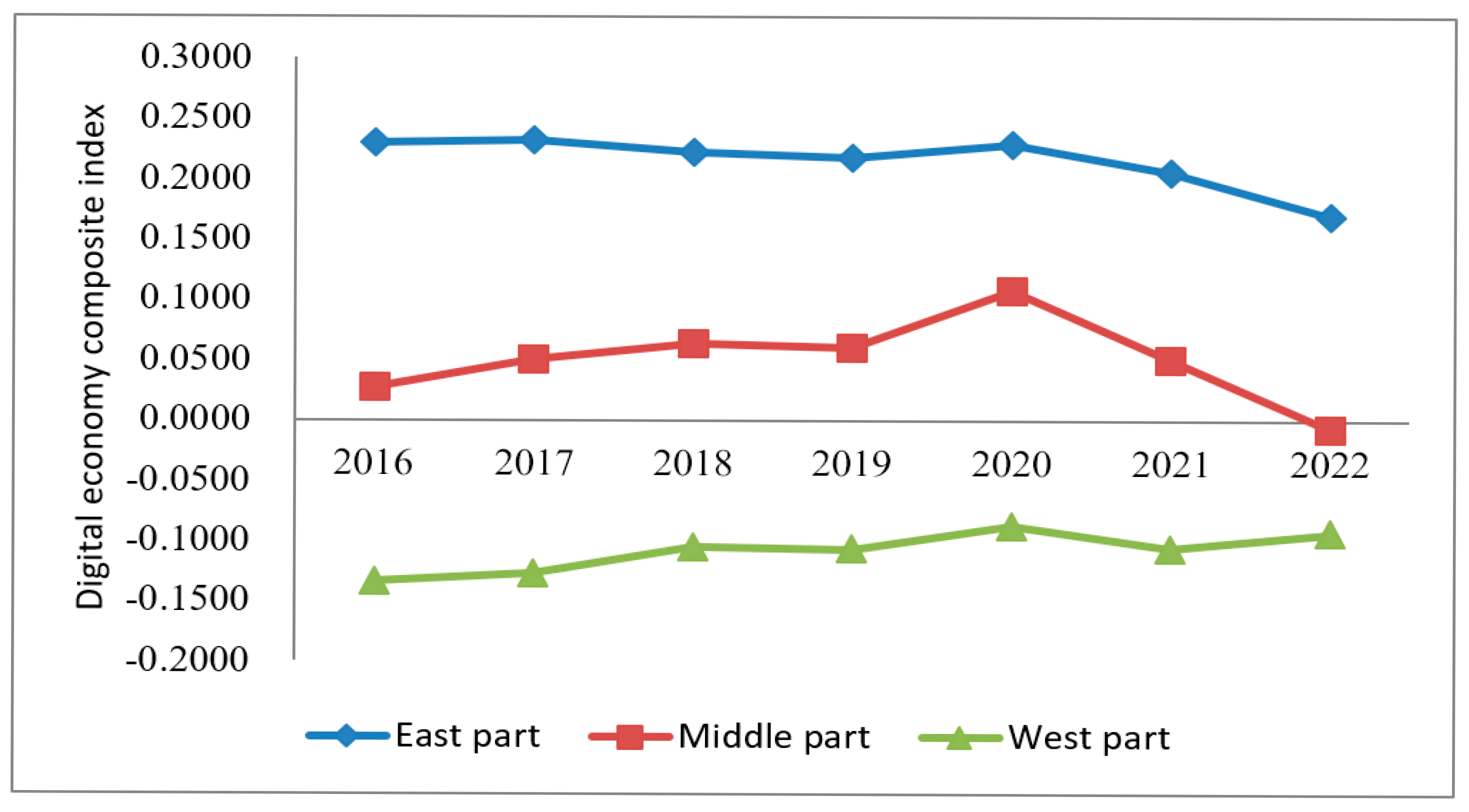
Figure 2 shows the comprehensive index of DE in three regions. As can be seen from Figure 2, during the investigation period, there were significant differences in the changing trend of the DE index in the three regions, among which the DE index in East China changed less, always higher than that in the central and western regions. The DE index in Central China has shown a downward trend, and it is lower than that in the western region in most years. The DE index in West China is characterized by slow climbing, and the development gap with the central region is widening. It demonstrates that during the period of 2016–2022, the development of DE presented the law of sequential decline in the eastern, western and central regions. On the one hand, this may be due to differences in digital infrastructure and technological accumulation. The eastern regions started building digital infrastructure earlier, with well-developed 5G networks, data centers and industrial internet, providing a solid foundation for the development of the digital economy. In contrast, the central and western regions face significant shortcomings in information network coverage and computing power distribution, which constrain the rapid growth of the digital economy. On the other hand, the eastern regions are dominated by high-end manufacturing and modern service industries, where enterprises have a strong willingness to undergo digital transformation and benefit from diverse technological application scenarios. The central regions have a high proportion of manufacturing, but the pace of digital transformation is relatively slow. Meanwhile, the western regions primarily rely on resource-based industries, with a lower penetration of the digital economy, making it difficult to achieve economies of scale.

5.1.2. The Analysis of the Calculation Results of OPMI

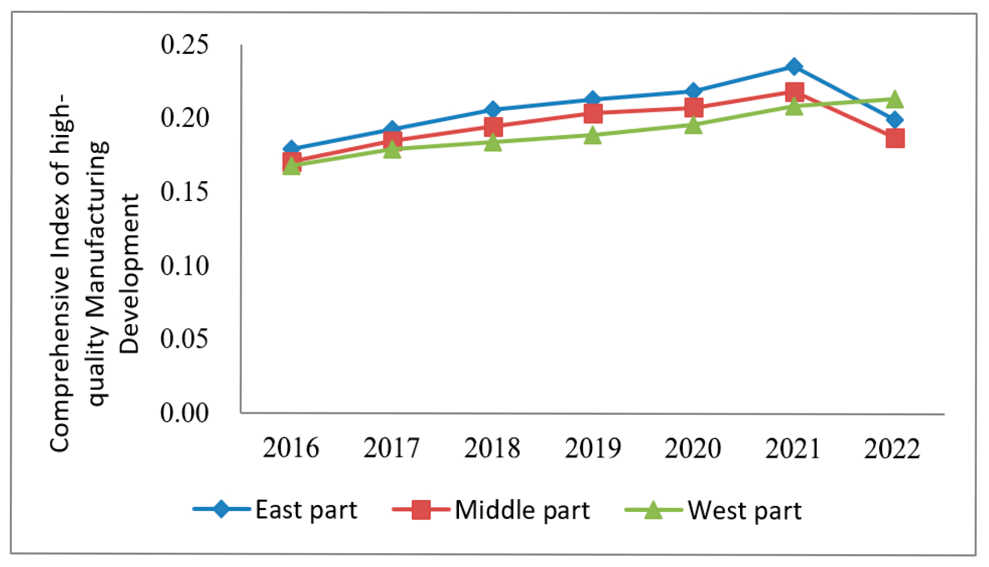
The comprehensive index value of OPMI in 30 provinces was calculated based on the entropy right TOPSIS method (see

Table 5. Comprehensive index of OPMI of 30 provinces.

District	2016	2017	2018	2019	2020	2021	2022	Mean Value
Beijing	0.270	0.256	0.271	0.299	0.278	0.293	0.126	0.274
Tianjin	0.156	0.176	0.209	0.209	0.224	0.211	0.376	0.188
Hebei	0.115	0.125	0.124	0.128	0.131	0.137	0.222	0.123
Shanxi	0.122	0.116	0.115	0.116	0.114	0.121	0.200	0.117
Nei Monggol	0.172	0.167	0.164	0.162	0.159	0.172	0.209	0.166
Liaoning	0.159	0.176	0.181	0.181	0.156	0.154	0.688	0.174
Jilin	0.159	0.170	0.147	0.164	0.153	0.164	0.210	0.160
Heilongjiang	0.150	0.138	0.127	0.121	0.102	0.100	0.184	0.134
Shanghai	0.170	0.169	0.178	0.189	0.197	0.211	0.221	0.177
Jiangsu	0.367	0.475	0.501	0.538	0.557	0.590	0.157	0.470
Zhejiang	0.251	0.277	0.315	0.342	0.373	0.387	0.143	0.296
Anhui	0.122	0.137	0.143	0.155	0.168	0.185	0.124	0.139
Fujian	0.155	0.164	0.170	0.175	0.176	0.189	0.104	0.166
Jiangxi	0.088	0.094	0.094	0.092	0.094	0.104	0.122	0.092
Shandong	0.244	0.278	0.303	0.316	0.329	0.349	0.120	0.285
Henan	0.131	0.134	0.189	0.195	0.205	0.205	0.080	0.162
Hubei	0.131	0.140	0.148	0.157	0.163	0.172	0.113	0.144
Hunan	0.138	0.144	0.153	0.157	0.174	0.182	0.143	0.148
Guangdong	0.397	0.447	0.456	0.474	0.504	0.619	0.287	0.444
Guangxi	0.140	0.146	0.151	0.163	0.174	0.192	0.192	0.150
Hainan	0.131	0.121	0.184	0.134	0.171	0.214	0.174	0.143
Chongqing	0.142	0.118	0.118	0.135	0.180	0.165	0.108	0.128
Sichuan	0.132	0.137	0.139	0.144	0.142	0.145	0.173	0.138
Guizhou	0.135	0.143	0.133	0.144	0.147	0.157	0.175	0.139
Yunnan	0.141	0.141	0.144	0.144	0.149	0.153	0.166	0.143
Shaanxi	0.160	0.154	0.141	0.146	0.134	0.138	0.220	0.150
Gansu	0.145	0.146	0.141	0.126	0.122	0.123	0.606	0.140
Qinghai	0.144	0.153	0.120	0.107	0.110	0.113	0.420	0.131
Ningxia	0.101	0.141	0.102	0.096	0.107	0.114	0.215	0.110
Xinjiang	0.158	0.152	0.147	0.151	0.141	0.144	0.216	0.152

). The results showed that China’s OPMI in most provinces did not greatly increase during the sample period. Among them, the majority of cities and provinces in 2022 were the central and western provinces, and the majority of cities and provinces were the eastern cities and provinces. Provinces and cities, such as Gansu, Qinghai, Ningxia and Shanxi, showed an increase in results, while Jiangsu, Beijing, Shandong and Zhejiang declined significantly. This may be due to the fact that the eastern regions, constrained by resource endowment, primarily rely on external energy supply. In recent years, restrictions on the use of high-carbon energy have increased, driving the energy structure towards cleaner alternatives, which has significantly impacted some high-energy-consuming manufacturing industries. In contrast, the central and western regions have relatively favorable resource endowments, especially with abundant coal, wind and solar energy resources. Under the support of national policies in recent years, these regions have accelerated the development of the new energy industry. Some areas have also built energy internet and smart grids, improving energy utilization efficiency.

Figure 3 shows the comprehensive index of OPMI in the three regions. We can find that the variations in the OPMI in the three regions are basically the same, all showing a trend of fluctuation. Among them, the annual growth rate of OPMI in the western region has reached 4.15%, significantly higher than that in the eastern region (1.81%) and central region (1.62%). The western region was 0.214 in 2022, with an average annual growth rate, indicating that OPMI in the western region increased more rapidly than that in the eastern and central regions. During the research period, the OPMI in the central region was the slowest. From the perspective of regional comparison, the average value of OPMI in the eastern region is the highest, reaching 0.207, followed by the central region (0.196) and the western zone (0.194). This phenomenon can be analyzed from two aspects. On the one hand, it is due to the base effect and catch-up effect. The starting point of OPMI in the western regions is relatively low. Therefore, with the diffusion of technology and policy support, the western regions can learn from the advanced experiences of the developed eastern regions, adopt more mature energy-saving technologies and green production models and are more likely to achieve higher growth rates, which is the “latecomer advantage”. On the other hand, industrial structure and policy guidance are also important factors contributing to this phenomenon. In recent years, the government has strongly promoted the development of the western regions and the “carbon peak and carbon neutrality” strategy, accelerating the green transformation of the manufacturing industry in the western regions. At the same time, the proportion of renewable energy, such as wind and solar power, applied in industrial production in the western regions has also continuously increased. Although the growth rate of OPMI in the western regions is relatively fast, its overall level is still lower than that in the eastern regions, indicating that further efforts are needed to promote technological upgrades and optimize industrial structure in order to continue narrowing the gap in energy utilization efficiency between regions.

5.2. Estimation Results of the Spatial Model

5.2.1. Spatial Correlation Test

GMI is used to investigate the global spatial correlation of DE and OPMI in various provinces. GMI is used for the spatial autocorrelation between DE and OPMI to determine whether they have spatial aggregation effects. If the GMI is significantly positive, it indicates that DE and OPMI show a positive spatial correlation, i.e., the level of digital economy development and energy optimization tend to converge in regions that are adjacent or have similar economic characteristics. This suggests that the digital economy may have spatial spillover effects on energy optimization through mechanisms such as technology diffusion and industrial synergy.

It can be seen from

Table 6. The global spatial correlation test results.

Year	DE		OPMI
	${\mathit{W}}^{\mathit{d}}$	${\mathit{W}}^{\mathit{e}}$	${\mathit{W}}^{\mathit{d}}$	${\mathit{W}}^{\mathit{e}}$
2016	0.063 ***	0.060 ***	−0.043	−0.034
2017	0.053 **	0.054 ***	−0.029	−0.021
2018	0.021	0.032 **	0.022	0.024 *
2019	0.011	0.026 *	0.030 *	0.033 *
2020	0.049 **	0.054 **	0.044 **	0.045 **
2021	0.021	0.032 **	0.050 **	0.054 **
2022	0.003	0.015	0.018	0.050 **

Note: ***, **, and * indicate significance at the 1%, 5% and 10% levels, respectively.

that in most years, the GMI of DE and OPMI are both positive and have passed the significance test, which means that the levels of DE and OPMI among various regions in China are not completely randomly distributed, but show an overall spatial correlation. Therefore, it is certain that the spatial effects should be fully considered in the study of China’s DE affecting OPMI. In addition, compared with the geographical distance weight, the GMI statistics under the economic distance weight are normally higher, which further shows that areas with homologous economic characteristics are more inclined to interactively affect DE and OPMI. Regions with similar levels of economic development often have similar industrial structures and development paths, especially in the context of the high integration of manufacturing and the digital economy, where the industrial agglomeration effect enhances interregional interaction. The development of the digital economy typically relies on infrastructure, technological innovation and talent mobility, and these resources tend to flow and diffuse between regions with similar economic characteristics, creating a strong regional linkage effect.

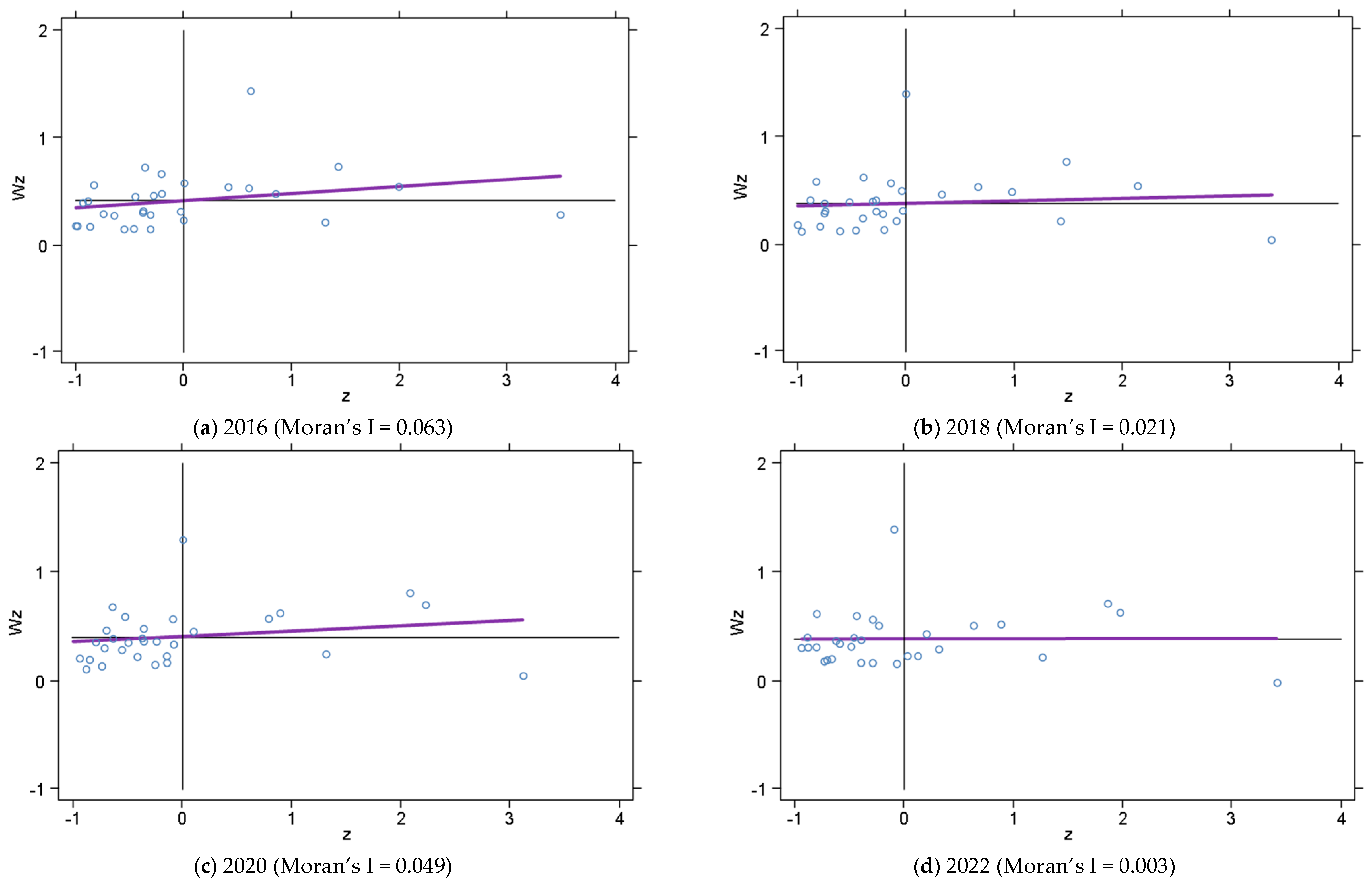
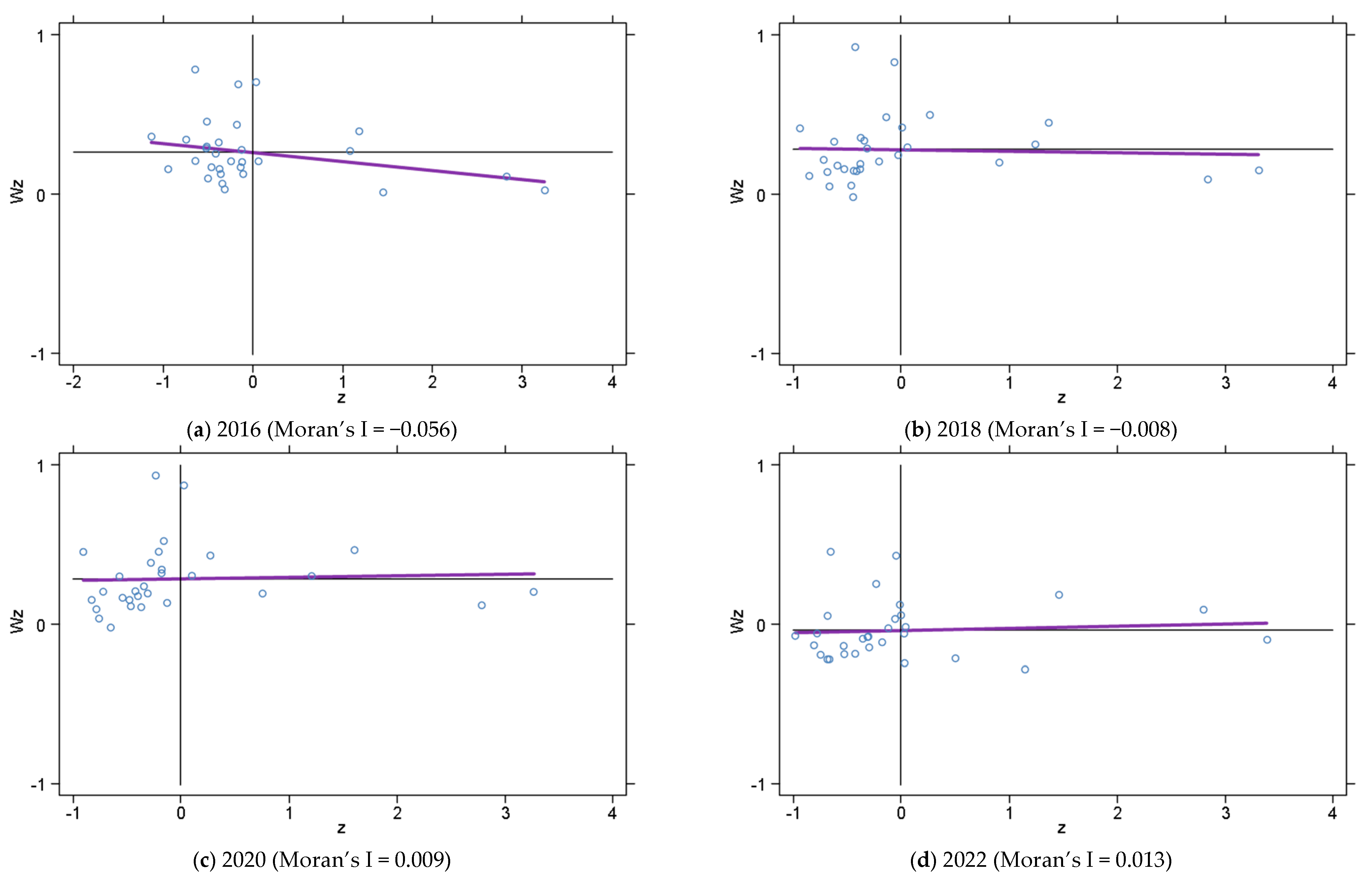
To further illustrate the local spatial correlation between DE and the optimization and upgrading of OPMI in China, Moran’s I scatter plots were employed, as depicted in Figure 4 and Figure 5. The sample regions were categorized into four quadrants, with a significant number of provinces positioned in the first (HH) and third (LL) quadrants.

First Quadrant (HH—High-High Clustering): This represents regions with a strong DE presence that are adjacent to other areas exhibiting similarly high levels. Jiangsu, Shanghai, Zhejiang, Fujian and Liaoning belong to this category.

Third Quadrant (LL—Low-Low Clustering): This cluster consists of provinces where DE remains underdeveloped, surrounded by regions with similarly low DE levels. Examples include Sichuan, Chongqing, Qinghai, Yunnan and Gansu.

Second Quadrant (LH—Low-High) and Fourth Quadrant (HL—High-Low): These indicate negative spatial correlation patterns, meaning that areas with contrasting DE levels are adjacent. Provinces such as Anhui, Hebei, Shandong, Inner Mongolia and Hainan fall into these categories.

As shown in Figure 4, the proportion of provinces falling within the HH and LL quadrants was recorded at 63.3% in 2016 and 2018, 70.0% in 2020 and 56.7% in 2022, demonstrating a clear positive spatial correlation in DE. Similarly, Figure 5 reveals that the proportion of provinces displaying strong local spatial agglomeration for OPMI—where high levels of OPMI cluster together and low levels do the same—stood at 53.3% in 2016, 63.3% in 2018 and 2020 and 60.0% in 2022. These findings reinforce the argument that both DE and OPMI exhibit significant spatial dependencies, contradicting the assumption of homogeneity and independence traditionally employed in econometric analyses. Consequently, ignoring spatial effects may introduce bias into empirical assessments. Therefore, employing spatial econometric models is essential for a more accurate evaluation of these relationships.

5.2.2. The Estimation Results of Spatial Effect

To determine the specific form of the spatial measurement model, this paper first performs OLS estimation on the panel data model without spatial effects and determines the SLM or the SEM by LM test.

Table 7. Regression results of spatial econometric model.

Variable	SLM				SEM				SDM
	${\mathit{W}}^{\mathit{d}}$		${\mathit{W}}^{\mathit{e}}$		${\mathit{W}}^{\mathit{d}}$		${\mathit{W}}^{\mathit{e}}$		${\mathit{W}}^{\mathit{d}}$		${\mathit{W}}^{\mathit{e}}$
	C	P	C	P	C	P	C	P	C	P	C	P
DE	0.046	0.22	0.029	0.14	0.032	0.11	0.030	0.13	0.311 *	0.06	0.273 *	0.09
HC	−0.043	0.55	0.007	0.75	0.007	0.75	0.008	0.70	0.148	0.64	0.249	0.41
OPEN	0.002 *	0.06	0.002 ***	0.00	0.002 ***	0.00	0.002 ***	0.00	0.007	0.22	0.007	0.21
IND	0.000	0.88	0.000	0.84	0.000	0.82	0.000	0.86	0.001	0.91	−0.004	0.69
UR	−0.007 *	0.08	−0.003 **	0.03	−0.003 **	0.02	−0.003 **	0.03	−0.014	0.60	−0.005	0.83
FIN	0.109 ***	0.00	−0.027 **	0.04	−0.029 **	0.03	−0.028 **	0.04	0.436 ***	0.00	0.499 ***	0.00
TEC	0.001	0.52	0.004 ***	0.00	0.004 ***	0.00	0.004 ***	0.00	0.008	0.30	0.014 *	0.07
MAR	0.011	0.40	−0.002	0.84	−0.002	0.86	−0.003	0.78	0.068	0.29	0.042	0.49
GOV	−0.003	0.38	0.001	0.64	0.001	0.60	0.001	0.62	0.010	0.56	0.005	0.74
W$\times$DE									3.517 ***	0.00	3.253 ***	0.00
$\rho$/$\lambda$	0.468 ***	0.00	−0.212	0.32	0.240	0.27	−0.009	0.97	−0.380	0.20	−0.278	0.32
sigma2	0.003 ***	0.00	0.007 ***	0.00	0.007 ***	0.00	0.007 ***	0.00	0.049 ***	0.00	0.049 ***	0.00
Provincial fixed	YES		NO		NO		NO		YES		YES
Year fixed	NO		YES		YES		YES		YES		YES

Note: C stands for the coefficient; P stands for the p-value; * p < 0.1, ** p < 0.05, *** p < 0.01.

shows the regression results of the spatial econometric model. The results indicate that both the LM statistics and the robust LM test reject the non-spatial models, supporting the suitability of the Spatial Lag Model (SLM) and the Spatial Error Model (SEM) under the adjacent spatial weight matrix. Given the general significance of the Spatial Durbin Model (SDM), it is appropriate to directly estimate spatial effects using this model. This further confirms the presence of a significant spatial correlation between provincial DE and OPMI, highlighting the necessity of employing a spatial econometric model to examine the impact of DE on OPMI.

Second, the LR test was conducted on the fixed effects of the SDM to determine whether the model required spatial or temporal fixed effects. The results indicate that both spatial and temporal fixed effects are necessary, confirming the appropriateness of a two-way fixed effects model. The subsequent Hausman test was used to select between fixed and random effects models, and its results rejected the null hypothesis at the 5% significance level, indicating that the fixed effects model should be adopted for parameter estimation.

Finally, the LR test was applied to assess whether the SDM could be simplified into either the SLM or SEM. The results rejected the null hypothesis at the 1% significance level, confirming that the SDM is the most suitable choice for spatial econometric estimation. The spatial distribution patterns of provincial DE and OPMI in China are not random, as evidenced by the model specification tests. Therefore, failing to account for spatial correlation when analyzing the influencing factors of provincial OPMI could result in biased estimation results.

Model estimation results show that under the two weight matrixes, regional DE has a significant contribution to regional OPMI in the region and passes the significance test at the 10% level, while the impact of DE on the OPMI in adjacent regions is significantly positive. Namely, the DE will not only promote local OPMI but also improve OPMI in adjacent regions. Considering that the results obtained by using the point estimation method of the spatial econometric model to test for the existence of the spillover effect of spatial variables are biased, this paper decomposes the effects of the explanatory variables on the explained variables into direct and indirect effects by using the method of partial differentiation according to their sources. Limited to space,

Table 8. Spatial effect decomposition.

Effect	${\mathit{W}}^{\mathit{d}}$		${\mathit{W}}^{\mathit{e}}$
	Coefficient	p Value	Coefficient	p Value
Direct effect	0.262	0.12	0.236	0.15
Indigo effect	2.659 ***	0.01	2.677 ***	0.01
Total effect	2.921 ***	0.01	2.913 ***	0.01

Note: *** p < 0.01.

only shows the spatial effect of DE on OPMI.

The results indicate that the direct effect of DE, measured under the geographical distance weight matrix, is positive but does not pass the significance test. This suggests that while DE contributes to the enhancement of OPMI within a region, its direct impact is not statistically robust. A possible explanation is that enterprises undergoing digital transformation often face challenges such as inadequate infrastructure, a shortage of skilled professionals, insufficient data availability and rigid organizational structures and corporate cultures that struggle to adapt to digital trends. Additionally, although DE enhances resource allocation efficiency in manufacturing-related activities such as research and development, production and trade, industrial development is often constrained by redundant construction, excessive investment and limitations on achieving high-quality manufacturing growth. In contrast, the indirect effect of DE on OPMI is positive and statistically significant at the 1% level. This finding implies that advancements in DE within one region can facilitate OPMI improvements in neighboring areas. A plausible reason is that the rapid development of DE promotes the efficient transfer of technology, information and other critical resources across regions, thereby accelerating the diffusion of innovation and enhancing technological efficiency and progress in adjacent areas. Moreover, as spatial interactions intensify, DE itself exhibits a spatial spillover effect, meaning that improvements in DE within one region can drive similar advancements in nearby regions. This dynamic fosters coordinated manufacturing development across geographically connected areas. Therefore, DE development not only enhances OPMI within a region but also generates positive external spillover effects, contributing to OPMI growth in adjacent areas through its radiation effect. In addition, the estimated results of DE affecting OPMI under the $W^d$ is basically consistent with that under the $W^d$.

5.3. The Estimation Results of Threshold Effect

DE has technical characteristics with considerable comprehensive reach and penetration, showing that it may have nonlinear threshold effects. This research adopts a panel threshold model to explore whether the contribution of the regional DE to OPMI has a “threshold effect”, that is, whether OPMI has undergone significant mutations with the changes in the development level of DE.

According to the Hansen study, the threshold effect test was first used to judge the number of thresholds. In this paper, one threshold and two thresholds are set to test the threshold effect of the threshold model, respectively, and the F-value and p-value obtained by the bootstrap method are shown in

Table 9. Panel threshold effect test.

Threshold Variable	Threshold Number	RSS	MSE	F Value	p Value	10%	5%	1%
DE	Single threshold test	0.9327	0.0046	38.50 ***	0.0000	9.0188	11.0112	15.2310
	Double threshold test	0.9143	0.0045	4.09	0.4600	8.9221	11.3174	17.4984

Note: The p-values and cut-off values in the table are the results obtained by repeated sampling 1000 times by the Bootstrap method; Note: *** p < 0.01.

.

As can be found in Table 9, the F value of the single threshold effect test of DE is 38.50, and the concomitant probability is 0.0000. The null hypothesis is rejected, indicating the existence of a single threshold. The double-threshold test was continued with an F-test value of 4.09 and a concomitant probability of 0.4600, accepting the null hypothesis and indicating that no double-threshold existed. Therefore, it can be considered that there is a single threshold effect of DE on OPMI. The estimates and corresponding 95% confidence intervals for the single threshold were 1.4339 and [1.3769, 1.4829], respectively.

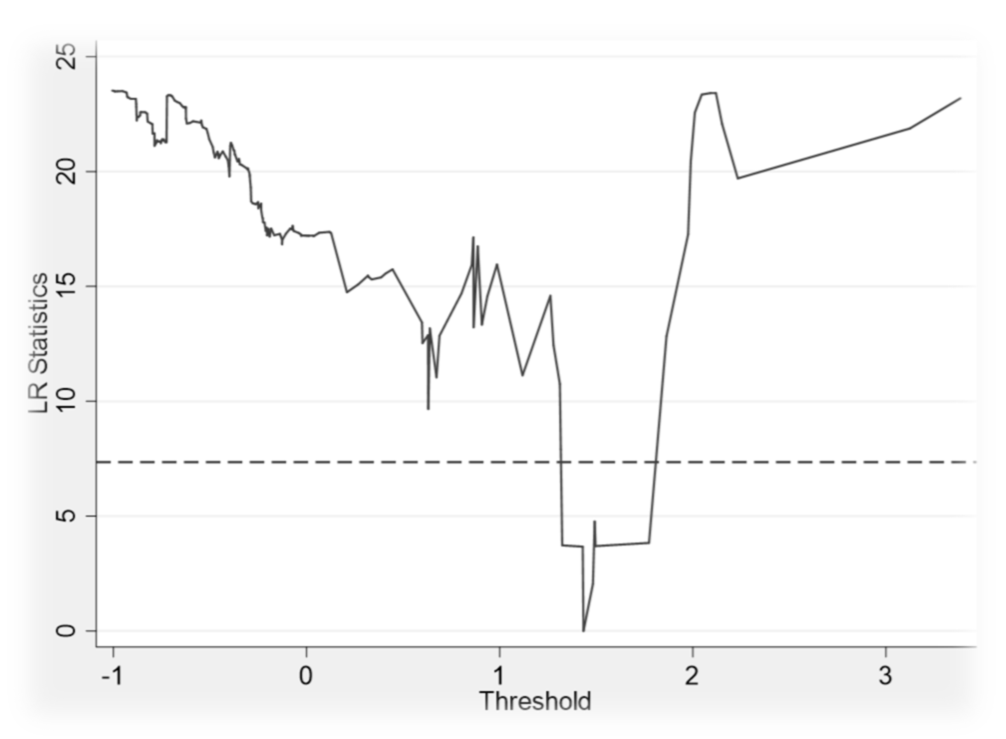
Drawing the likelihood ratio function (LR) diagram by Stata 17.0 can more accurately reflect the construction process of threshold values and confidence intervals. Figure 6 shows the estimation value for single thresholds and its confidence intervals. The estimate of the threshold parameter is the value taken when LR equals 0, and 1.4339 in the single-threshold model. The 95% confidence interval for this threshold is the interval formed by the critical value of 7.35 for all LR values less than the 5% significance level (see Figure 6).

This paper divides the corresponding sample interval according to the threshold value and then estimates the influence coefficient of DE on OPMI in different intervals. The regression results of the threshold model in

Table 10. Regression results of panel threshold model.

Coefficient	Estimated Value	Standard Error	T-Value	p-Value	95% Confidence Interval
DE < 1.4339	0.0517 ***	0.0188	2.74	0.007	0.0145	0.0889
DE ≥ 1.4339	−0.0635 **	0.0248	−2.56	0.011	−0.1125	−0.0146
HC	−0.0261	0.0209	−1.25	0.215	−0.0674	0.0153
OPEN	0.0008 *	0.0004	1.94	0.055	0.0000	0.0016
IND	−0.0013	0.0010	−1.30	0.195	−0.0033	0.0007
UR	−0.0027 *	0.0016	−1.73	0.085	−0.0058	0.0004
FIN	0.0158	0.0157	1.01	0.316	−0.0152	0.0467
TI	0.0069 ***	0.0015	4.68	0.000	0.0040	0.0098
MAR	0.0078	0.0115	0.68	0.496	−0.0148	0.0305
GOV	−0.0007	0.0016	−0.45	0.652	−0.0038	0.0024
_CONS	0.3203 ***	0.0933	3.43	0.001	0.1361	0.5045
F value	19.28 ***			0.000
R-squared	0.5314

Note: * p < 0.1, ** p < 0.05, *** p < 0.01.

show that if DE is below the threshold value 1.4339, the estimated coefficient is 0.0517, and passes the significance test at 1% level, indicating that the development of DE will drive the growth in the level of OPMI. When the DE index exceeds 1.4339, the estimated coefficient is −0.245 and passes the significance test at 5% level, indicating that as the level of DE grows further, it will lead to a decline in the level of OPMI. This may be due to resource misallocation caused by the development of the digital economy. As the level of DE rises rapidly, resources such as information technology, capital and labor may become highly concentrated in the digital industry, resulting in insufficient resource supply for the manufacturing sector. For example, a large amount of capital and talent flows into the digital industry, which restricts the technological upgrading and green transformation investments required for OPMI. In addition, some traditional manufacturing enterprises, during their digital transformation process, may face issues such as inadequate technical adaptability due to a lack of precise policy guidance and proper resource allocation, leading to an inability to synchronize improvements in energy efficiency and even a decline in energy utilization efficiency.

It can be inferred that there is an obvious inverted “U” relationship between the development of DE and OPMI, and the corresponding inflection point value is DE index 1.4339. Therefore, it can be proved that the impact of DE on OPMI has a significant nonlinear threshold effect.

It is also possible to divide the study sample into two zones based on this single threshold, namely low level of digital economy development (DE < 1.4339) and high level (DE ≥ 1.4339). The problem of inter-regional variation due to the evolution of the panel data over time needs to be taken into account; therefore, the average value of the DE index for each province from 2016 to 2022 is used to divide the intervals, and it is found that the only provinces in the high-level zone are Beijing, Shanghai and Zhejiang, while the rest of the provinces are in the low-level zone. In addition, the provinces are also divided into zones for the 2022 Digital Economy Composite Index, and it was found that the provinces in the high and low digital economy development zones were consistent with the results divided by the mean value of the Digital Economy Composite Index. This shows that the development of DE in most provinces in China is in a relatively reasonable range, and the rapid development of DE in this range still has a significant positive effect on promoting China’s OPMI. Therefore, in order to promote OPMI, paying attention to the stable and healthy development of DE is what we need to do further.

6. Discussions

This study identifies both similarities and differences when compared to existing research.

Consistent with the spatial economic characteristics observed in China, there is noticeable regional heterogeneity in DE levels. Specifically, DE in East China is significantly higher than in the central and western regions, with the western region exhibiting the lowest level. This finding aligns with the conclusions of Zou and Deng (2022) [56]. The rapid growth of DE in East China can be attributed to its thriving information technology sector and well-established policy framework. In contrast, Central and West China face limitations in digital knowledge and information accessibility, leading to comparatively lower DE levels.

While an increase in regional DE directly promotes OPMI within the same region, the effect does not pass the significance test. However, DE has a significantly positive spillover effect on OPMI in neighboring regions, a result consistent with the findings of Ma and Zhu (2022) [57] and Wu et al. (2024) [13]. Furthermore, there exists an inverted U-shaped nonlinear relationship between DE and OPMI. It is worth noting that Ma and Zhu (2022) [57] suggest that regional DE exerts a positive nonlinear influence on OPMI.

The above findings confirm that DE positively impacts OPMI. However, the specific mechanisms through which DE influences OPMI remain to be further explored. Therefore, it is essential to investigate the pathways through which DE indirectly drives OPMI.

7. Conclusions and Policy Implications

Taking the provincial panel data from 2016 to 2022 as the research sample, the space spillover effect and threshold effect of DE on OPMI are empirically analyzed.

(1)

There are obvious regional differences in DE and OPMI in China. Among them, the east region has a higher degree of DE, while the level of DE in the central and west regions is both lower and close to each other. The level of OPMI shows a decreasing pattern in the east, central and west regions in that order.

(2)

OPMI and DE are not both randomly distributed, but both have significant spatial correlation. The direct effect of DE on OPMI is positive but not significant, and the indirect effect and total effect are significantly positive, that is, DE has not had a significant effect in promoting OPMI in this region, but has a significant positive space spillover effect on OPMI in adjacent areas.

(3)

DE has an obvious threshold effect on OPMI, which is not a simple linear relationship. A lower level of DE can help to promote OPMI, but when the level of DE crosses the inflection point, it will inhibit OPMI.

According to the research conclusions, make the following recommendations:

First, improve the DE system and policy guarantee, establish and improve an efficient DE market system. Do a good job in top-level design and enhance the government governance capacity. Specifically, government departments should strengthen the construction of digital infrastructure. Enhance the carrying capacity of the digital economy by pushing forward the layout of new types of infrastructure such as 5G networks, industrial Internet and data centers. Expand broadband and mobile network coverage in remote areas to narrow the digital divide. At the same time, it will implement a mechanism for feeding talent and technology. Implementing the “digital enclave” model, encouraging eastern enterprises to set up R&D centers or branches in central and western China. Tax incentives and subsidies will be used to promote technological spillover.

Second, in order to speed up OPMI, it is integral to give full play to the spatial spillover effect of DE, break the regional administrative barriers of the flow of factors, promote the benign interaction of DE in neighboring regions, strengthen information sharing, talents and technology among neighboring regions, and carry out exchanges and cooperation among neighboring regions.

Third, pay attention should be paid to the threshold effect of DE on OPMI, control the development speed of DE within a reasonable range, scientifically allocate DE resources according to different regional economic development levels in order to promote OPMI.