Abstract
Under the “dual-carbon” strategic framework, the installed capacity of renewable energy sources has continuously increased, while that of conventional generation units has progressively decreased. This structural shift significantly diminishes the operational flexibility of power generation systems and intensifies grid imbalances caused by renewable energy volatility. To address these challenges, this study proposes a carbon-aware multi-timescale virtual power plant (VPP) scheduling framework with coordinated multi-energy integration, which operates through two sequential phases: day-ahead scheduling and intraday rolling optimization. In the day-ahead phase, demand response mechanisms are implemented to activate load-side regulation capabilities, coupled with information gap decision theory (IGDT) to quantify renewable energy uncertainties, thereby establishing optimal baseline schedules. During the intraday phase, rolling horizon optimization is executed based on updated short-term forecasts of renewable energy generation and load demand to determine final dispatch decisions. Numerical simulations demonstrate that the proposed framework achieves a 3.76% reduction in photovoltaic output fluctuations and 3.91% mitigation of wind power variability while maintaining economically viable scheduling costs. Specifically, the intraday optimization phase yields a 1.70% carbon emission reduction and a 7.72% decrease in power exchange costs, albeit with a 3.09% increase in operational costs attributable to power deviation penalties.
1. Introduction
With the intensification of the global energy crisis and the increasingly severe environmental pollution problem, renewable energy power generation has attracted widespread global attention. Among them, wind power and photovoltaic power generation have developed more rapidly. However, they exhibit stochastic and fluctuating characteristics. To ensure the safety of power grid operation when integrating new energy into the grid, the prediction and consumption technologies of wind power output and photovoltaic power generation have received extensive global attention.
As a technology that can aggregate and flexibly schedule and control distributed energy, the virtual power plant (VPP) ensures the stable operation of the power system. It is also regarded as a supportive technology for increasing the proportion of renewable energy and achieving the “dual carbon” target. Reference [1] introduces the framework of synergistic utilization among carbon capture plants, power-to-gas facilities, and gas units in VPPs to enhance the flexible dispatch and consumption of wind/photovoltaic (PV) renewable energy generation. Reference [2] constructs an optimal combined heat and power scheduling model for virtual power plants to further improve the consumption capacity of new energy. Reference [3] addresses the energy loss caused by cyclic renewable conversion and multi-stakeholder conflicts in integrated energy systems (IESs) by proposing a hierarchical optimization framework with a two-layer architecture. Reference [4] presents a source-load-storage coordinated energy management model for microgrids, enabling full-time collaborative optimization across internal and external boundaries. Compared with traditional integrated energy systems, virtual power plants can respond to grid scheduling commands in real time by relying on intelligent algorithms and edge computing technologies. On the one hand, this allows for efficient cooperation with various distributed resources; on the other hand, it reduces the computational pressure resulting from the centralized control of traditional integrated energy systems. Currently, there are relatively few studies on the uncertainties of renewable energy generation and the load side in VPPs, and most of them use deterministic models as the basis for optimal dispatch.
Regarding source-load uncertainty analysis, current research mainly includes stochastic planning, robust optimization, fuzzy optimization, and rolling time-domain methods. In reference [5], fuzzy theory is introduced to fuzzily parameterize uncertain quantities such as wind power generation and load, and a coordinated optimal scheduling model for wind-power-photovoltaic-carbon-capture virtual power plants is constructed. Reference [6] proposes a source-load-storage coordinated energy management model for microgrids with full-time collaborative optimization, considering real-time pricing and time-of-use mechanisms. Reference [7] proposes a new uncertainty model for wind power generation and analyzes source-load uncertainty using scenario reduction with scenario simplification. However, since scenario generation mainly relies on the probability density function, its error is relatively large. In reference [8], a flexible optimal dispatch model of a virtual power plant based on multiple wind energy prediction results is constructed to cope with the volatility and uncertainty of wind energy resources. Reference [9] combines the Wasserstein metric with the characteristics of a combined electric and thermal system, conducting in-depth research and optimization on source-load uncertainty. Reference [10] proposes a two-stage robust optimization method to describe the uncertainty of new energy output, aiming to improve scheduling efficiency and economic benefits. Reference [11] uses a distributionally robust optimization approach to describe the optimal scheduling of electrically–thermally coupled systems, taking new energy uncertainties into account, with the goal of enhancing the scheduling economy and reliability. Nevertheless, robust optimization often models the worst-case scenario, which is conservative and less economical.
To address the above problems, this paper focuses on modeling the uncertainty of wind power output in virtual power plants using information gap decision theory (IGDT). IGDT is a non-probabilistic and non-fuzzy mathematical method for handling uncertainty quantification that is more effective in situations with high uncertainty or insufficient data information. One of its applications is to assist decision-makers in maximizing or minimizing the acceptable uncertainty range relative to a fault based on the prediction target value, thereby ensuring that the prediction does not fall below the minimum pre-determined outcome. Reference [12] proposes a joint multi-source scheduling strategy based on IGDT to address the multi-parameter uncertainty on the source-load side of the system. Reference [13] combines information gap decision theory (IGDT) with a dynamic time-of-day tariff model to address the gap nature of distributed power output and power fluctuations caused by the disordered charging behavior of a large number of electric vehicles (EVs). Reference [14] combines the confidence intervals of the Gaussian mixed probability model with information gap decision theory to achieve the optimal scheduling of integrated energy systems. Reference [15] formulates a complementary operation optimization decision model for multi-energy systems based on the information gap decision theory approach to address the impact of the uncertainty of wind power and photovoltaic output on system scheduling. Reference [16] proposes an optimization strategy for carbon capture and power-to-gas conversion based on information gap decision theory to achieve the optimal dispatch of integrated energy systems with low-carbon economy. Reference [17] proposes a hybrid approach including stochastic planning and IGDT to enable 100% consumption of renewable energy sources in microgrids.
To further reduce the carbon emissions of virtual power plants, step-by-step carbon trading is introduced to incentivize the source side to increase the proportion of renewable energy generation. Reference [18], aiming to achieve low-carbon economic dispatch, proposes integrating the stepped carbon trading mechanism into the low-carbon economic dispatch model of the integrated electricity–gas–heat energy system to realize the low-carbon and economic operation of the system. Reference [19] introduces stepped carbon trading to enable the integrated energy system to participate in the carbon trading market with lower carbon emissions. Reference [20] proposes an optimal dispatch strategy with the objective function of minimizing the sum of carbon trading costs, purchased gas and coal consumption costs, carbon sequestration costs, unit startup and shutdown costs, and wind power curtailment costs. Reference [21] proposes an innovative optimal scheduling strategy to achieve the dual objectives of low carbon emissions and efficient energy utilization, comprehensively balancing the low-carbon characteristics of the integrated energy system and the complexity of multi-energy load response characteristics.
However, all the above-mentioned studies only consider the optimal scheduling strategy in the day-ahead stage and do not take into account the impact of short-term new energy output and load variations on the system. To solve this problem, this paper introduces an intraday rolling optimization strategy, which adjusts the output plan based on ultra-short-term new energy output and load forecasts. Currently, some scholars have conducted research on intraday rolling optimization scheduling. Reference [22], in response to new energy output fluctuations, establishes a three-stage optimization scheduling model for integrated energy systems, including day-ahead, intraday rolling, and real-time adjustment, coupled with power-to-gas and carbon capture. Reference [23] establishes a three-stage optimization model with day-ahead, intraday rolling, and real-time adjustment to gradually optimize unit output for the imbalance between energy supply and demand caused by fluctuations in new energy generation and customer load. Reference [24] proposes a dual column-and-constraint generation (dual C&CG) algorithm for robust optimization with decision-dependent uncertainties (DDUs) in power systems. This algorithm overcomes the limitations of traditional methods for decision-independent uncertainties, and theoretical proofs ensure its convergence and optimality. Reference [25] addresses the challenge of optimal scheduling of virtual power plants for the integration of photovoltaics with flexible loads such as chilled water storage air conditioners and electric vehicles. This paper proposes a new approach by modeling the light stochastic dynamics through stochastic differential equations and using a hybrid logistic dynamic model to handle the decision-making for air conditioners and electric vehicles and then solves the problem using a rolling time-domain method. However, the fluctuation of new energy output is not described in detail, and there is a large deviation between the pre-day output plan and the intraday output.
The increasing penetration of renewable energy sources poses a significant challenge to virtual power plants (VPPs) in balancing supply and demand uncertainty and coordinating multiple energy sources. Existing studies often fail to adequately address the coordinated operation of carbon capture systems with power-to-gas/hydrogen fuel cell (P2G-HFC) technologies, while conventional optimization methods struggle to balance day-ahead robustness and intraday adaptability. To address these shortcomings, three contributions are made in this study:
- (1)
- A novel multi-energy VPP integration framework is proposed. This framework combines a carbon capture device, a P2G, and a hydrogen fuel cell system for bidirectional energy conversion and cascading carbon utilization, aiming to reduce carbon emissions.
- (2)
- Compared with the traditional P2G system, the IGDT robust model based on wind and light uncertainty analysis proposed in this paper can avoid the impact of wind and light fluctuations on the operation of the system. The new energy consumption is improved, and compared with the traditional model, the new energy consumption rate is increased by 6.66% to 98.75%.
- (3)
- Compared with the traditional IGDT model, this paper proposes a multi-timescale model and uses the IGDT robust model in the day-ahead stage to improve the day-ahead schedule margin by taking into full consideration the wind power volatility and to reduce the adjustment of the day-ahead schedule based on the short timescale.
2. VPP System Architecture
The VPP model proposed in this paper is shown in Figure 1. It includes a carbon capture power plant, combined heat and power (CHP) unit, gas boiler, wind turbine, photovoltaic power plant, hydrogen fuel cell (HFC), electric boiler, electric refrigeration unit, absorption chiller, power-to-gas device (P2G), as well as thermal energy storage, electric energy storage, and gas energy storage systems. The electric load is mainly supplied by the CHP unit, carbon capture power plant, wind turbine, photovoltaic power plant, hydrogen fuel cell, and the charging and discharging of electric energy storage. The heat load is mainly met by the CHP unit, gas boiler, electric boiler, hydrogen fuel cell, and the charging and discharging of thermal energy storage. The gas load is mainly supplied by the gas purchased from the upper-level gas network.
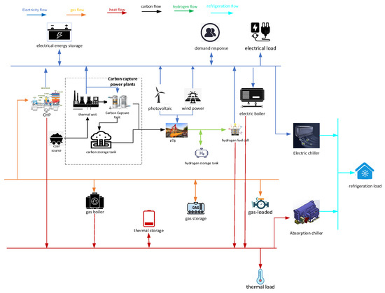
Figure 1.
VPP system structure.
The P2G and energy storage systems, as flexible scheduling units of the VPP with excellent time-shifting characteristics, can consume excess wind and photovoltaic power generation. This paper selects a two-stage P2G device. In the first stage, water is electrolyzed to produce hydrogen, which provides fuel for the hydrogen fuel cell. Meanwhile, it serves as a preparation for the reaction between carbon dioxide and natural gas in the second stage.
2.1. Stepped Carbon Trading Model
The carbon trading mechanism refers to a system where, in order to reduce carbon emissions, the government department assigns carbon emission targets to enterprises based on the previous year’s power generation. Thus, enterprises with lower carbon emissions can sell their excess carbon emissions in the carbon trading market to generate revenue, while enterprises with higher carbon emissions need to purchase carbon allowances from the carbon trading market. The traditional carbon trading price is relatively fixed, and it is not very effective in motivating enterprise users to reduce carbon emissions. Therefore, this paper introduces the ladder-carbon-trading mechanism to encourage enterprises to reduce carbon emissions. The ladder-carbon-trading model mainly includes the carbon emission quota model, the actual carbon emission model, and the ladder-carbon-emission-trading model [18,19].
2.1.1. Carbon Emission Quota Modeling
In this paper, the carbon emission allowances of the virtual power plant mainly include those from the CHP unit, gas boiler, carbon capture power plant, and the electricity purchased from the grid. The carbon emission allowances are mainly allocated through the method of gratuitous emission allowances, and this paper adopts the allowance–determination method in the literature [17]:
where is the carbon emission allowance of the VPP at time , is the carbon emission allowance obtained by the CHP unit for electricity supply, is the carbon emission allowance obtained by the CHP unit for heat supply, is the carbon emission allowance obtained by the thermal unit in the carbon capture power plant for electricity supply, and is the carbon emission allowance obtained by the gas boiler unit for heat supply.
2.1.2. Real Carbon Emissions Modeling
Carbon emissions from thermal units in a carbon capture power plant in a VPP system are partially absorbed by the carbon capture unit and therefore need to be taken into account.
where is the actual carbon emission of the VPP at time t, is the actual carbon emission of the CHP unit for electricity generation, is the actual carbon emission of the CHP unit for heat generation, is the actual carbon emission of the carbon capture plant, is the actual carbon emission of the gas boiler unit for heat supply, and is the carbon emission of the purchasing unit for electricity from the grid.
2.1.3. Laddered Carbon Trading Models
In the above model, according to the formula, the actual carbon emissions and carbon emission quotas can be obtained. Finally, the amount of carbon emissions for its participation in the carbon trading market can be calculated:
where is the amount of carbon allowances participating in the market.
In order to better motivate carbon emission reductions, this paper proposes the use of a stepped carbon trading mechanism to constrain carbon emissions.
where iis the cost of carbon trading at time t (positive denotes the purchase of carbon credits, negative denotes the sale of carbon credits), is the base price of carbon trading, is the growth price of carbon trading, is the length of the carbon emission interval, and is the compensation price of carbon trading.
The laddered carbon trading diagram is shown in Figure 2, which visualizes the price of carbon trading rights in the carbon emission interval.
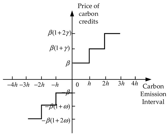
Figure 2.
Laddered carbon trading.
2.2. Carbon Capture Power Plant—P2G-HFC Framework
The carbon capture power plant in this paper consists of a conventional thermal power unit, a carbon capture device, and a carbon storage tank. The electricity for the carbon capture device is mainly supplied by the internal thermal power unit. Part of the carbon dioxide captured by the carbon capture device is stored in the carbon storage tank, and the other part is provided to the P2G device.
2.2.1. Carbon Capture Devices
The energy consumption of the carbon capture device , includes fixed energy consumption and operation energy consumption , and the operation energy consumption is related to the amount of carbon dioxide captured by the carbon capture device, with its formula shown below:
where is the energy consumption per unit mass of CO2 captured; ; and is the amount of captured by the carbon capture device at time .
In practice, the carbon capture device is unable to capture all of the generated by the thermal power unit, and its capture formula is shown below:
where is the capture efficiency of the carbon capture device, and is the amount of produced by the thermal power unit at .
2.2.2. Carbon Storage Devices
In this paper, the decoupling of the carbon capture plant from the P2G plant is realized by introducing a carbon storage device, with the storage equation shown below:
where is the carbon storage capacity of the carbon storage device at ; is the loss rate of the carbon storage itself; are the carbon storage charging and discharging efficiencies; are the storage charging and discharging powers at ; are the charging and discharging state variables taking the value of ; are the minimum and maximum values of the carbon storage capacity; and are the upper limits of carbon storage charging and discharging.
2.2.3. Thermal Power Units
In this paper, thermal power units are regarded as the main source of carbon emissions and also as the energy source for carbon capture devices. Part of the electricity generated by them is supplied to the carbon capture devices, and part of it is used to power other devices within the virtual power plant, as shown in the following equations:
where is the power generated by thermal power units at , and is the power supplied to the virtual power plant by the carbon capture power plant at .
where is the actual carbon emissions generated per unit of electricity supplied by the thermal power unit.
2.2.4. P2G Devices
Since the P2G plant has low efficiency in the actual process, in this paper, P2G is divided into two stages: electrical conversion to hydrogen (P2H) and methanation, with the equations shown as follows:
where is the power consumed by the P2G device to produce hydrogen at , is the power of hydrogen produced by the P2G at , and is the conversion efficiency of P2H. is the power of hydrogen consumed by methanization at , is the power of gas produced by methanization at , and is the efficiency of methanization. is the energy supplied by the wind turbine to the P2G device at , is the energy supplied by the photovoltaic power plant to the P2G device at , and are the energy supplied by the P2H and the energy supplied by the storage device at , respectively. The hydrogen energy supplied by the Power-to-Hydrogen(P2H) and the hydrogen storage unit at t, respectively.
In the methanation process, which consumes CO2 in a volume equal to the volume of methane produced, an equilibrium constraint needs to be added, which is given by the following equation:
where is the amount of consumed for methanation at , is the density of , is the calorific value of methane, is the calorific value per unit of electrical energy converted, and is the amount of deposited by P2G into carbon storage at .
2.2.5. HFC Equipment
In this paper, by adding the HFC equipment, it can generate electric power and thermal power by consuming P2G-produced hydrogen. Meanwhile, the thermal and electric conversion efficiencies of the HFC are adjustable with strong flexibility. Additionally, the combination of P2G devices can achieve a low-carbon economy with lower operating costs, and its formula is shown below:
where are the electric and thermal power outputs from the HFC device at time t; are the electric and thermal efficiencies of the HFC device; is the hydrogen power input to the HFC device at time ; , are the upper and lower limits of the hydrogen power input to the HFC device; , are the upper and lower limits of the hydrogen creep power input to the HFC device; are the upper and lower limits of the electric and thermal ratios of the HFC device; and are the upper and lower limits of the hydrogen energy supplied by hydrogen storage and the hydrogen energy supplied by the P2G device, respectively.
2.2.6. Hydrogen Storage Device
The energy storage model considering hydrogen losses is shown below:
where is the carbon storage capacity of the hydrogen storage device at ; is the loss rate of hydrogen storage itself; are the charging and discharging efficiencies of hydrogen storage; are the charging and discharging powers of the storage at time t; are the charging and discharging state variables (taking the value of {0,1}), respectively; are the minimum and maximum values of the hydrogen storage capacity; and are the upper limits of hydrogen storage charging and discharging, respectively.
2.3. Other Modules
2.3.1. CHP Units
The mathematical expression for a gas turbine is as follows:
where are the electric and thermal power outputs from the CHP unit at time t; are the electric and thermal efficiencies of the CHP unit; is the natural gas power input to the CHP unit at time t, , are the upper and lower limits of the electric power output from the CHP unit; , are the upper and lower limits of the thermal power output from the CHP unit; and , are the upper and lower limits of the natural gas creep from the CHP unit.
2.3.2. Gas Boilers
The gas boiler provides thermal power to the VPP with the following mathematical expression:
where is the thermal power output from the gas boiler at ; is the natural gas power input to the gas boiler at ; is the thermal power conversion efficiency of the gas boiler; , are the upper and lower limits of thermal power output from the gas boiler; and , are the upper and lower limits of natural gas creep into the gas boiler.
2.3.3. Electric Boiler Model
2.3.4. Modeling of Electrical, Thermal, and Gas Energy Storage
In this paper, electric, thermal, and gas energy storage devices are modeled similarly, so they are modeled uniformly:
where ; is the storage capacity of the storage device of the storage device at time ; is the loss rate of the storage; are the charging and discharging efficiencies of the n-type storage; are the charging and discharging powers of the n-type storage at time t; are the charging and discharging state variables of the n-type storage device at time t; , are the minimum and maximum values of the n-type storage capacity; and are the upper limits of the charging and discharging power of the n-type storage, respectively.
2.3.5. Modular Modeling of Cold Energy
2.4. Tariff-Based Demand Response Modeling
In this paper, time-of-use tariffs are used as a guide to model the elasticity coefficient of the electric load demand response, which is shown below:
where is the elasticity coefficient between the VPP load at time and the tariff at time i and also represents the row and mi column of the elasticity coefficient matrix at ; is the change in the load after and before demand response at the time of ; is the pre-demand response VPP load at time ; is the change in the tariff at time i; and is the original tariff at time i.
The tariff-based demand response model in this paper is shown below:
where is the VPP electrical load after demand response at time.
2.5. Constraints
2.5.1. Wind Power Output Constraints
2.5.2. Thermal Unit Output Constraints
2.5.3. Interaction Constraints with Electricity and Gas Networks
3. Optimization Model Based on IGDT Day-Ahead
In the day-ahead stage, this paper mainly takes 1 h as the time interval and introduces the IGDT robust model to analyze the uncertainty of renewable energy power generation and reduce the impact of renewable energy power generation fluctuations on the power system.
3.1. Day-Ahead Objective Function
The day-ahead stage mainly aims to minimize the operating cost of the VPP and determine the day-ahead output plan of each unit; its cost mainly includes the cost of stepped carbon trading, the cost of purchased electricity and gas, and the fuel cost of the carbon capture plant.
where is the current VPP operating cost; are the current VPP electricity and gas purchase costs, respectively; is the current carbon capture plant fuel cost; and is the current VPP ladder carbon trading cost.
- (1)
- Day-Ahead gas purchase cost
- (2)
- Day-Ahead power purchase costs
- (3)
- Day-Ahead Carbon Capture Power Plant Fuel Costs
- (4)
- Day-Ahead stepped carbon trading costs
- (5)
- Day-Ahead power balance constraints
The power balance constraints in this paper mainly include the electrical power balance, gas power balance, and thermal power balance constraints.
where is the VPP thermal power demand at ; is the VPP gas power demand at ; is the VPP gas power demand at ; and is the VPP cold power demand at .
3.2. IGDT Robust Optimization Model Before VPP Day
The IGDT model can be divided into the robustness model (RM) and the opportunity model (OM). Since the RM can circumvent the unfavorable influence of uncertainty on the VPP, this paper adopts the RM to describe the operation of each unit before the VPP day.
The VPP optimization model can be described as
where is the VPP objective function; is the VPP equilibrium constraint; is the VPP disequilibrium constraint; is the decision variable; and is the uncertainty variable.
Robust Optimization Model
Since the above IGDT model is a two-layer model, according to its principle, it models the fluctuations in wind power and photovoltaic (PV) output within the information gap interval. When the output of wind turbines and photovoltaic power plants is lower than their robustness, to improve calculation efficiency, the model can be simplified to the following formula:
where and are the predicted values of the WTG and PV power output at , respectively. is the deviation coefficient of the PV power plant output.
Since the IGDT model can only solve for a single variable, it needs to be singularized for multiple variables: multiple uncertain variables are first normalized and then given weight coefficients for singularization.
where and are the robustness and chance deviation coefficients for solving the variable IGDT in a single WTG; and are the robustness and chance deviation coefficients for solving the variable IGDT in a single PV plant output; and are the corresponding weight coefficients of and .
4. Intraday Rolling Model
In this paper, the intraday rolling model is used to further adjust the day-ahead capacity model. On the basis of day-ahead dispatching, the timescale is changed from 1 h to 15 min to further forecast the intraday load and renewable energy capacity. The period is shortened to 4 h, and based on the day-ahead scheduling, rolling optimization of equipment operation is conducted. The equipment capacity is derived from this rolling optimization with a 15 min time interval.
4.1. Intraday Objective Function
During the intraday rolling phase, adjustments need to be made based on the previous day’s equipment output, and deviation penalty costs are introduced to reduce large deviations in output.
where is the intraday VPP operating cost; are the intraday VPP purchased electricity and gas cost, respectively; is the intraday carbon capture plant fuel cost; is the intraday VPP laddered carbon trading cost; and is the penalty cost for the deviation of the intraday from the previous day’s VPP.
- (1)
- Intraday gas purchase cost
- (2)
- Intraday power purchase costs
- (3)
- Intraday Carbon Capture Power Plant Fuel Costs
- (4)
- Intraday stepped carbon trading costs
- (5)
- Deviation penalty costs
4.2. Intraday Constraints
In the intraday rolling phase, the constraints are the same as before the day, that is, mainly the change in equipment output.
- (1)
- Electrical balance constraints
- (2)
- Thermal power balance
- (3)
- Gas power balance
In the formula, is the power of the interaction between the VPP and the gas network at in the day; is the output gas power of the electric-to-gas conversion device at in the day; are the power of the gas storage discharge and filling at in the day; is the predicted gas load of the VPP at in the day; is the gas power consumed by the CHP unit at in the day; and is the gas power consumed by the gas boiler at in the day.
- (4)
- Cold power balance
In the formula, is the intraday electric chiller output at moment t output cold power, is the intraday absorption chiller output at moment t output cold power, and is the intraday short timescale predicted t cold load.
5. Example Analysis
5.1. Solution Flow
The solution flow of this paper is shown in Figure 3. In the day-ahead phase, with 1 h as the timescale and 24 h as the time period, based on the IGDT robust model, the objective function of the day-ahead phase is solved using the Gurobi 10.0 solver in MATLAB, which results in the planned output of the VPP in the day-ahead phase; in the intraday phase, with 15 min as the timescale and 4 h as the period, rolling optimization is applied according to the ultra-short-term wind power, PV output, and load forecasts. In the intraday phase, rolling optimization is applied to solve the optimization based on the ultra-short-term wind and PV power and load forecasts, and the intraday power plan is adjusted based on the day-ahead VPP power plan.
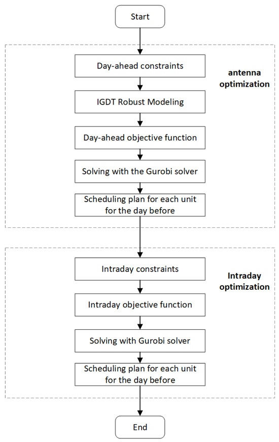
Figure 3.
Solution flow.
5.2. VPP Model Data
In order to verify the validity of the model built in this paper, the VPP system includes a wind turbine, a PV plant, a CHP unit, a carbon capture plant, an HFC, a gas boiler, an electric-to-gas conversion unit, and an electric boiler. The data of each equipment are shown in Table 1, the predictions of various types of loads are shown in Figure 4, and the predicted output of renewable energy is shown in Figure 5. As in References [22,26], the natural gas price is shown in Table 2. the time-share electricity and gas prices are shown in Table 3 and Table 4. A cross-reference to the energy alphabet in the text can be found in Appendix A Table A1.

Table 1.
Parameters of each model of VPP.
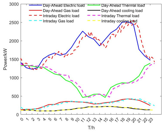
Figure 4.
Load forecast chart.
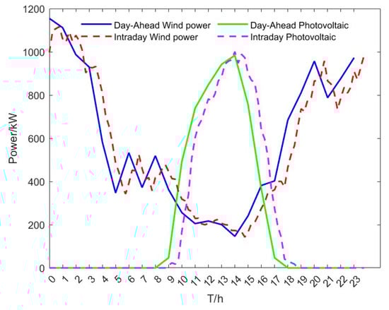
Figure 5.
Wind power photovoltaic forecast.
Table 2.
Time-of-day gas prices.
Table 3.
Time-of-day tariffs.
Table 4.
Changes in electricity prices before and after demand response.
5.3. Comparative Analysis of Models
In the day-ahead stage, in order to verify the superiority of the proposed scheme in this paper, the analysis is carried out through three scenarios. (1) The optimized scheduling model in this paper removes the demand response and the IGDT robust optimization. (2) The VPP in this paper includes a deterministic model of demand response. (3) The VPP includes demand response and stochastic programming models. (4) The VPP includes robust optimization models for demand response. (5) The VPP model in this paper.
As shown in Figure 6, compared to the original load data, the load after demand response, without changing the user demand for electricity at the same time, reduces the peak hour 18:00–19:00 h and 9:00–12:00 h loads and improves the load in the valley hours to effectively consume new energy generation.
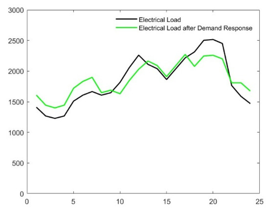
Figure 6.
Demand response effect diagram.
As illustrated in Table 5, Scenario 1 exhibits a relatively high electricity procurement cost during peak hours due to the absence of demand response (DR) mechanisms and the neglect of renewable energy output uncertainty. Consequently, the procurement cost in Scenario 1 is 1.93% higher compared to Scenario 2. In Scenario 2, the incorporation of DR results in a decrease of 4.18% and 2.12% in the electricity and gas procurement costs, respectively, indicating that electric load DR can effectively reduce operational costs.
Table 5.
Scheduling results for each scenario in the previous day.
In contrast to the first two scenarios, Scenario 3 incorporates a stochastic programming model to analyze renewable energy output uncertainty. Compared to the robust model in Scenario 4 and the interval-based generalized decision-making theory (IGDT) robust model in Scenario 5, Scenario 3 demonstrates a cost reduction. However, when addressing the uncertainty of renewable energy output, the accuracy of Scenario 3 tends to be lower with fewer generated scenarios, while the computational complexity increases significantly and the calculation time is extended with more scenarios. Scenario 4 yields the highest costs, primarily because to fully mitigate the impact of renewable energy uncertainty, it increases electricity and gas procurement, leading to higher costs. Additionally, as electricity procurement rises, so does carbon trading, ultimately elevating the overall cost.
Scenario 5 represents the method employed in this study, which not only maintains robustness but also reduces computational complexity. By introducing fluctuation intervals, Scenario 5 achieves a 3.08% cost reduction compared to the robust model. This approach balances robustness and computational efficiency, providing a practical solution to the challenges posed by renewable energy uncertainty.
5.4. Analysis of VPP Day-Ahead Scheduling Results
To evaluate the performance of the proposed day-ahead model, the methods from existing studies [22,23] were comparatively analyzed with the approach developed in this work. Notably, Reference [22] neglects renewable energy uncertainty in its power dispatch analysis while adopting a stepwise carbon pricing mechanism, whereas Reference [23] lacks uncertainty quantification of renewable generation with fixed carbon pricing assumptions. The simulation results are systematically summarized in Table 6.
Table 6.
Comparative analysis of models.
Since this paper adopts the IGDT robust model to characterize the uncertainty of wind power, the cost increases by 1.73% and 2.05% compared with References [22,23] without uncertainty characterization, but the new energy consumption rate increases by 6.66% and 4.57%, respectively. As Reference [23] does not adopt ladder carbon trading, the cost of carbon trading increases by 24.40% and 15.22%, and the rate of new energy consumption decreases by 4.57% and 2.19% compared with the scheme proposed in this paper and Reference [22], respectively.
In order to verify the effectiveness of the IGDT day-ahead scheduling strategy and the impact of new energy output uncertainty on the VPP scheduling strategy, this paper sets the robust factor and analyzes it through different weight coefficients of the IGDT robust model, and its results are shown in Table 7.
Table 7.
IGDT robust model bias with different weight coefficients.
From the table, it can be seen that the radius of fluctuation of a single uncertainty is different under different weighting coefficients due to different sensitivities of wind and light output fluctuations. At the same time, the uncertainty radius of the VPP system increases with the increase in the difference of the weighting coefficients, and the overall uncertainty radius of the VPP is minimized at . The scheduling manager can adjust the weighting coefficients to achieve the optimal scheduling result according to the actual situation.
In this paper, we use to determine that the dispatch cost boundaries of the IGDT robust model at that moment are , the uncertainty radius of the PV output , the uncertainty radius of the wind turbine output , and the uncertainty radius of the VPP system . This indicates that the actual PV output fluctuates within a range of 3.76% compared to the predicted output, while the actual WT output fluctuates within a range of 3.91% compared to the predicted output, and the total cost does not exceed . Compared with the deterministic model, the IGDT robust model has a certain conservatism and its scheduling cost increases. Its scheduling results are shown in Figure 7, Figure 8, Figure 9 and Figure 10.
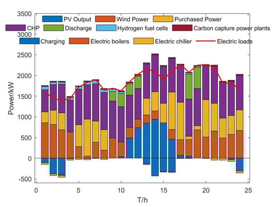
Figure 7.
Power dispatch optimization results.
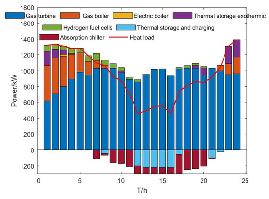
Figure 8.
Thermal power scheduling optimization results.
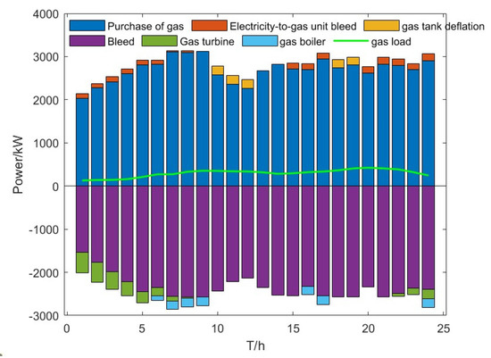
Figure 9.
Results of gas power optimization scheduling.
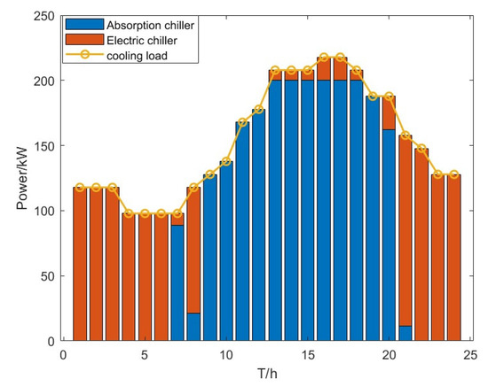
Figure 10.
Cold power optimization results graph.
In order to achieve the lowest daily dispatch cost for the VPP system, the output profile of each unit varies with the time-of-day electricity and gas prices. In the VPP system, the electrical loads are mainly supplied by the external grid and internal CHP units, wind turbines, photovoltaic plants, HFCs, and storage units; the thermal loads are mainly met by the gas boilers, electric boilers, and heat storage units; the cooling loads are supplied by electric and absorption chillers; and the gas loads are mainly met by natural gas purchased from the external grid and supplemented by electricity-to-gas units.
In the trough period from 23:00 to 04:00 the next day, the demand for electricity load is low. During this period, electricity and gas prices are low, and wind turbine output is high. To leverage the benefit of purchasing electricity from the grid, excess electricity is used to charge the electric energy storage device. At the same time, since the demand for heat energy is higher in this period, the heat supply is mainly achieved through the regulation of electric boilers, gas boilers, and cogeneration units, as well as the exothermic regulation of heat storage. Natural gas purchased from the external gas network during this period is mainly supplied to the CHP and gas boilers, and demand is met by regulating the gas output from the electricity-to-gas converter.
During the peak period from 9:00 to 12:00, PV generation increases from zero due to the time-of-day profile (not directly linked to price or wind output). The electrical load during this period is mainly supported by adjusting the CHP units and discharging storage. Meanwhile, the heat power demand decreases: the heat load is mainly supported by the CHP units, with the thermal storage adjusted for load balancing; the gas load is higher, met by natural gas purchased from the external grid and gas storage discharge; and the cold load demand increases, partly satisfied by consuming heat energy and partly by using power from lower-cost periods.
During the 13:00–18:00 period, when electricity demand and electricity/gas prices decline, the grid purchases large quantities of electricity to fully charge the storage units in preparation for subsequent peak consumption hours, maximizing profits. As the heat load demand is lowest during this period, the thermal energy storage unit stores excess heat from the CHP unit, while the electricity-to-gas unit discharges gas.
In the VPP system, the output of each unit is constantly adjusted to minimize dispatch costs, primarily driven by fluctuations in electricity and gas prices. The combination of the electricity-to-gas (P-to-G) plant and the carbon capture plant not only reduces carbon emissions but also lowers the fuel costs of hydrogen fuel cells and gas units via the E-to-G process while consuming excess renewable energy output. This realizes the economic and low-carbon operation of the VPP.
5.5. Analysis of VPP Intraday Scheduling Results
In this paper, we adopt the two-stage optimization scheduling strategy of “day-ahead IGDT–intraday rolling optimization”, and the results of the two-stage optimization scheduling are shown in Table 8.
Table 8.
Intraday optimization and intraday scheduling optimization.
As shown in the above table, the implementation of ultra-short-term wind and PV output and load forecasting in the intraday phase reduces carbon emissions by 1.70% and power interaction costs by 7.72% compared to the day-ahead phase. This shows that intraday rolling optimal dispatch can effectively reduce carbon emissions and power exchange costs in a virtual power plant (VPP) system. However, it is worth noting that the operating costs increase by 3.09% due to the inclusion of a deviation penalty factor in the intraday phase. When the actual output of each unit deviates significantly from the day-ahead dispatch result, the penalty cost increases accordingly.
To reduce the output deviation between the day-ahead and intraday phases, a robust model based on the Interval Generalised Distribution Transform (IGDT) is used in the day-ahead scheduling phase. This model minimizes the difference between the two phases. In addition, ultra-short-term forecasts in the intraday phase further address the uncertainties associated with the wind and PV output and load. In contrast, independent day-ahead scheduling provides relatively coarse scheduling results due to its wide timescales. The introduction of a deviation penalty factor through intraday rolling optimization allows for further refinement of the output schedule for each unit, thus reducing the deviation.
Figure 11 shows the results of day-ahead optimal scheduling and intraday rolling optimization for the VPP system units. A comparative analysis of the exchanged power with the grid shows that the VPP’s intraday power procurement plan strictly adheres to the day-ahead procurement plan, resulting in minimal differences in interaction costs between the two time periods, thus reducing the daily operating costs of the VPP system. Similarly, the results of the interaction with the natural gas grid show that the day-ahead natural gas procurement plan is highly aligned with the day-ahead power procurement plan, supporting the VPP’s natural gas, power, and heat requirements. The power and heat output schedules of the combined heat and power (CHP) units show a close correspondence between day-ahead and intraday schedules, thus meeting the VPP’s power and heat needs.
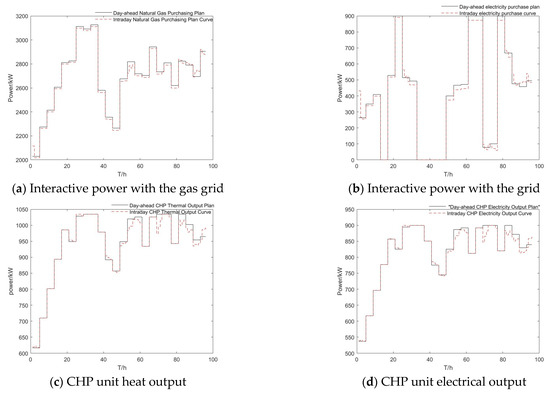
Figure 11.
Intraday optimized scheduling with intraday rolling optimization results.
5.6. Comparative Analysis of Model Solving Performance
To comprehensively analyze the superiority of different solution methods, particle swarm optimization (PSO), genetic algorithm (GA), and sparrow search algorithm (SSA) are selected for comparative analysis with the Gurobi solver used in this paper (only for the model proposed herein). The computational performance comparison is presented in Table 9.
Table 9.
Computational performance of solving stochastic mixed-integer linear programming.
As shown in Table 9, the Gurobi solver achieves 100% optimality accuracy for the mixed-integer linear programming problem, demonstrating the absolute advantage of commercial solvers in exact solutions. However, its solution time is longer than that of traditional heuristic algorithms: it increases by 26.09%, 17.39%, and 30.43% compared to PSO, GA, and SSA, respectively. This reflects the typical trade-off between solution efficiency and accuracy between exact solvers and heuristic algorithms: Gurobi ensures global optimality through exhaustive search, while heuristic algorithms exhibit significant advantages in computational speed using heuristic rules, making them suitable for large-scale optimization problems sensitive to solution time.
6. Conclusions
In order to realize the low-carbon economic operation of the VPP system, this paper proposes a multi-energy coupled dispatch model of electricity-heat-gas-cooling, puts forward a two-phase optimal dispatch strategy based on IGDT’s day-ahead optimal dispatch and intraday rolling optimal dispatch, and draws the following conclusions through the analysis of the arithmetic examples:
- (1)
- New energy consumption and carbon emission reduction are achieved through the electricity-heat-gas-cooling multi-energy coupling model. In the former stage, by introducing the information difference theory and the tariff-based demand response model, the arithmetic demand response can effectively guide users to shave the peaks and fill the valleys to achieve load shifting and reduce the pressure on the supply of the VPP, and the IGDT robust model takes into account the fluctuation of the new energy output, which improves the stability of the power supply of the VPP system.
- (2)
- In the intraday phase, a rolling optimal dispatch strategy is adopted to introduce intraday short-term wind and light output and load forecasts and to adjust the output plan of each unit of the VPP before the day to further reduce the actual error and carbon emission.
- (3)
- Through the analysis of arithmetic examples, the intraday output plan is operated strictly in accordance with the day-ahead output plan to reduce the cost of plan adjustment in the case of meeting the user’s demand.
Author Contributions
W.Z.: constructed the model structure of the virtual power plant, established the overall framework of the paper, and wrote the manuscript. J.L.: constructed the mathematical model of each module of the virtual power plant and constructed the solution process and uncertainty description method for the day-ahead model. J.Z.: established the design scheme of the intraday adjustment model. H.L.: comparative analysis of algorithms. C.S.: data collection and conclusion preparation. Q.A.: improved the thesis, so that the experiment could be carried out smoothly. M.C.: improved the flaws in the experiment. Translated with DeepL.com (free version). All authors have read and agreed to the published version of the manuscript.
Funding
The author(s) declare that financial support was received for the research, authorship, and/or publication of this article. This research was funded by the project “Research and Application of Regional Scale User-Side Resource Collaboration and Interaction Technology” (090000KC22120002).
Data Availability Statement
The data used in this article have been given in detail in the article for the reader’s reference.
Acknowledgments
The authors are extremely grateful to each of the authors who have helped and contributed to this paper. It is their joint efforts that allowed this paper to be successfully published.
Conflicts of Interest
Authors Wanling Zhuang, Junwei Liu, Jun Zhan and Honghao Liang were employed by the company Shenzhen Power Supply Company. The remaining authors declare that the research was conducted in the absence of any commercial or financial relationships that could be construed as a potential conflict of interest.
Appendix A
Table A1.
Letter meaning.
Table A1.
Letter meaning.
| Letter | Meaning |
| electrical energy | |
| heat energy | |
| natural gas | |
| hydrogen | |
| carbon energy | |
| cold energy |
References
- Sun, H.; Liu, Y.; Peng, C.; Meng, J. Optimal scheduling of a virtual power plant with carbon capture and waste incineration taking into account power-to-gas synergy. Grid Technol. 2021, 45, 3534–3545. [Google Scholar]
- Yuan, G.; Liu, H.; Yu, J.; Liu, J. Optimal scheduling of combined heat and power in a virtual power plant with carbon capture cogeneration units. Chin. J. Electr. Eng. 2022, 42, 4440–4449. [Google Scholar]
- Gao, Y.; Ai, Q.; He, X.; Fan, S. Coordination for regional integrated energy system through target cascade optimization. Energy 2023, 276, 127606. [Google Scholar] [CrossRef]
- Gao, Y.; Ai, Q. Novel Optimal Dispatch Method for Multiple Energy Sources in Regional Integrated Energy Systems Considering Wind Curtailment. CSEE J. Power Energy Syst. 2024, 10, 2166–2173. [Google Scholar]
- Zhong, W.; Huang, S.; Cui, Y.; Xu, J.; Zhao, Y. Coordinated optimal tuning of wind-power-photovoltaic-carbon capture virtual power plant considering source-load uncertainty. Grid Technol. 2020, 44, 3424–3432. [Google Scholar]
- Gao, Y.; Ai, Q. Research on Demand Side Response Strategy of Multi-Microgrids Based on Improved Co-evolution Algorithm. CSEE J. Power Energy Syst. 2021, 7, 8–16. [Google Scholar]
- Rahimi, M.; Ardakani, F.J.; Ardakani, A.J. Optimal stochastic scheduling of electrical and thermal renewable and non-renewable resources in virtual power plant. Int. J. Electr. Power Energy Syst. 2020, 127, 106658. [Google Scholar] [CrossRef]
- Luo, Y.; Yang, H.; Niu, B.; Chang, G.; Meng, K. An intra-day rolling flexible optimal dispatch method for virtual power plants considering multiple wind energy forecast scenarios. Power Syst. Prot. Control 2020, 48, 51–59. [Google Scholar]
- Liu, H.; Li, H.; Ma, J. Distributionally robust optimal scheduling of combined electric-heat systems considering source-load uncertainty. Power Autom. Equip. 2023, 43, 1–8. [Google Scholar]
- Xin, X.; Li, Q.; Zhang, Q.; Liao, C. A Two-stage Robust Optimal Scheduling Method for Virtual Power Plants Taking into Account Multi-flexibility Resources. J. Eng. Therm. Energy Power. 2024, 39, 113–122. [Google Scholar]
- Liu, S.; Lu, Y.; Li, L.; Zhang, Z.; Sha, L. Electricity-gas-heat Coupled System Distributionally Robust Optimization Considering Uncertainty of New Energy Sources. Proc. CSU-EPSA 2024, 36, 109–120. [Google Scholar]
- Ye, H.; Liu, S.; Hu, J.; Xiong, X.; Tan, Y. Multi-source joint scheduling strategy of power system containing solar thermal power plant based on IGDT. Power Syst. Prot. Control 2021, 49, 35–43. [Google Scholar]
- Liao, J.; Zhang, Z.; Dou, C. Double-tier economic dispatch strategy for electric vehicle access to virtual power plant based on information gap decision theory and dynamic time-sharing tariff. Power Autom. Equip. 2022, 42, 77–85. [Google Scholar]
- Peng, C.; Zheng, C.; Chen, J.; Wang, C.; Zhou, X. Robust optimal scheduling of integrated energy system based on confidence gap decision-making. Chin. J. Electr. Eng. 2021, 41, 5593–5604. [Google Scholar]
- Liao, S.; Liu, H.; Liu, B.; Zhao, H.; Wang, M. An information gap decision theory-based decision-making model for complementary operation of hydro-wind-solar system considering wind and solar output uncertainties. J. Clean. Prod. 2022, 348, 131382. [Google Scholar] [CrossRef]
- Zhao, Z.; Bao, G.; Li, X. Optimization and Scheduling of Integrated Energy Systems with Carbon Capture and Storage-Power to Gas Based on Information Gap Decision Theory. Power Gener. Technol. 2024, 45, 651–665. [Google Scholar]
- Daneshvar, M.; Mohammadi-Ivatloo, B.; Zare, K.; Asadi, S.; Anvari-Moghaddam, A. A Novel Operational Model for Interconnected Microgrids Participation in Transactive Energy Market: A Hybrid IGDT/Stochastic Approach. IEEE Trans. Ind. Inform. 2020, 17, 4025–4035. [Google Scholar] [CrossRef]
- Cui, Y.; Zeng, P.; Zhong, W.; Cui, W.; Zhao, Y. Low-carbon economic dispatch of integrated electricity-gas-heat energy system considering stepwise carbon trading. Power Autom. Equip. 2021, 41, 10–17. [Google Scholar]
- Chen, J.; Hu, Z.; Chen, Y.; Chen, W. Thermoelectric optimization of integrated energy system considering stepped carbon trading mechanism and electric hydrogen production. Power Autom. Equip. 2021, 41, 48–55. [Google Scholar]
- Chen, D.; Liu, F.; Liu, S. Optimal scheduling of a virtual power plant with P2G-CCS coupling and gas hydrogen doping based on stepwise carbon trading. Grid Technol. 2022, 46, 2042–2054. [Google Scholar]
- Wang, R.; Cheng, S.; Liu, Y. Optimal scheduling of energy hub master-slave game based on integrated demand response and reward-penalty ladder carbon trading. Power Syst. Prot. Control 2022, 50, 75–85. [Google Scholar]
- Wang, H.; Zhou, K.; Wu, Z.; Zou, Z.; Li, X. Multi-timescale optimal scheduling of an integrated energy system with coupled power-to-gas and carbon capture. China Electr. Power 2024, 57, 214–226. [Google Scholar]
- Wang, Z.; Tao, H.; Cai, W.; Zhang, L.; Meng, J. Optimal scheduling study of multi-timescale rolling optimization in combined cooling, heating and power system. J. Sol. Energy 2023, 44, 298–308. [Google Scholar]
- Tan, T.; Xie, R.; Xu, X.; Chen, Y. A robust optimization method for power systems with decision-dependent uncertainty. Energy Convers. Econ. 2024, 5, 133–145. [Google Scholar] [CrossRef]
- Xu, Y.; Liu, Z.; Wen, F.; Palu, I. Receding-horizon based optimal dispatch of virtual power plant considering stochastic dynamic of photovoltaic generation. Energy Convers. Econ. 2021, 2, 45–53. [Google Scholar] [CrossRef]
- Zhang, T.; Guo, Y.-T.; Li, Y.-H.; Yu, L.; Zhang, J. Optimized scheduling of regional integrated energy systems taking into account electric-thermal integrated demand response. Power Syst. Prot. Control 2021, 49, 52–61. [Google Scholar]
Disclaimer/Publisher’s Note: The statements, opinions and data contained in all publications are solely those of the individual author(s) and contributor(s) and not of MDPI and/or the editor(s). MDPI and/or the editor(s) disclaim responsibility for any injury to people or property resulting from any ideas, methods, instructions or products referred to in the content. |
© 2025 by the authors. Licensee MDPI, Basel, Switzerland. This article is an open access article distributed under the terms and conditions of the Creative Commons Attribution (CC BY) license (https://creativecommons.org/licenses/by/4.0/).