Article

Control of Wind-Power Systems Operating at Variable Wind Speeds to Optimize Energy Capture

by
Cristian Paul Chioncel
1,
Samuel Ciucurita
2 and
Elisabeta Spunei
1,*
1
Department of Engineering Sciences, Faculty of Engineering, Babes-Bolyai University, 400028 Cluj-Napoca, Romania
2
Department of Automation and Applied Informatics, Politehnica University of Timisoara, 300006 Timisoara, Romania
*
Author to whom correspondence should be addressed.
Energies 2025, 18(10), 2574; https://doi.org/10.3390/en18102574
Submission received: 21 March 2025 / Revised: 23 April 2025 / Accepted: 14 May 2025 / Published: 15 May 2025
(This article belongs to the Section A3: Wind, Wave and Tidal Energy)

Abstract

:
This paper examines two contradictory aspects of wind turbine operation: the positive aspect of functioning at the maximum power point (MPP) and the negative aspect of power gaps that occur during significant fluctuations in wind speed. The analysis utilizes experimental data from a 2.5 MW wind turbine operating in the Dobrogea region, focusing on identifying the optimal energy zone. To maintain operation within this optimal zone, a control algorithm based on kinetic energies is developed. The control aims to adjust the load on the electric generator in relation to the wind speed value. The proposed approach ensures operation within the MPP through a control algorithm based on kinetic energies, which adjusts the load on the generator according to the wind speed values.

1. Introduction

According to the new strategies, the share of renewable energy in electricity is expected to reach 46% by 2030. Thus, in 2023, the global installed wind capacity was 1015 GW, with the construction of new wind capacities experiencing a 50% increase compared to 2022 [1]. In light of the growing number of wind farms [2], the use of variable generators in electricity production can aid in providing ancillary services, such as primary and secondary frequency regulation [3,4].
In both traditional wind systems and offshore installations, it is essential to monitor the maximum power point (MPP). For offshore systems, it is recommended to implement an integrated approach that includes an active rectifier and several passive rectifiers, in conjunction with a multi-port permanent magnet synchronous generator, to effectively manage the total output power [5].
This paper examines the operation of the wind turbine (WT) at the MPP, which corresponds to the optimal mechanical angular speed (MAS), ωOPTIM.
To ensure maximum wind energy capture, it is necessary to correlate wind speed with mechanical angular speed. For this, it is necessary to determine the maximum power of the wind turbine at different wind speeds over time [6,7].
Most wind systems function under fluctuating wind velocities, necessitating continuous control of the output power [8]. Different strategies are used to measure or estimate wind speed, such as:
-
Use of a low-power, no-load turbine at the mechanical angular velocity [9];
-
Nonlinear mapping, which involves measuring rotor speed, tilt angle and aerodynamic torque as perceived by the disturbance observer [10];
-
The assessment of turbine torque and rotor speed is conducted utilizing sliding mode observers grounded in nonlinear control theory, with the aim of calculating the effective wind velocity by reversing the aerodynamic model of the turbine [11];
-
The original signal is decomposed into multiple sequences, utilizing deep learning prediction models and neural network optimization [12].
Various control strategies are employed for wind turbines operating at variable wind speeds. One proposed approach involves the use of an extended optimal torque controller, which is structured upon the accurate assessment of wind speed through nonlinear mapping. Simulations have demonstrated that this method enhances the precision of effective wind speed estimation by 2–7% and improves electricity production efficiency by 0.35% [10]. Another control strategy focuses on maximizing the amount of wind energy harvested by utilizing the optimal power curve and the power curve corresponding to different wind speeds [13]. Additionally, other studies suggest that optimize energy extraction from a wind turbine utilizing a doubly fed induction generator (DFIG), a combination of maximum power point (MPP) tracking using a high-gain observer, and a second order sliding mode control for the DFIG is recommended [14].
Control strategies must consider various operational scenarios of wind turbines. Consequently, during rapid load discharges, the turbine rotor will accelerate beyond its nominal speed, potentially leading to the breaking of blades or damage to a component of the wind energy system. To address this issue, it is essential to restrict the discharge to a maximum value [15]. This limitation can be implemented based on the response trajectory characteristics of the system [16]. Additionally, in the operation of wind systems, the power oscillation damping regulator can influence the structural system of the turbine, producing effects that are either comparable to or less significant than those caused by fluctuations in wind speed [17]. Other issues that may impact the operation of wind systems can arise from atmospheric discharges that affect the turbine blades and certain internal components [18,19], or from unbalanced loads [20].
In the specialized literature concerning the field addressed [5,9], valid solutions for wind turbines to operate at maximum power point under optimal mechanical angular velocity, amidst variable wind speeds over time, have not been identified. Furthermore, the operational wind systems have not been evaluated in terms of energy efficiency [13,21].
This article addresses precisely the issue of maximizing wind energy capture under varying wind speeds over time. When wind speeds fluctuate, the wind turbine operates continuously in a dynamic mode, with variable rotational speeds [4,16,22].
Given the dynamic nature of the process, the equation for kinetic momentum [10,23] is utilized in the following manner:
J d ω d t = M W T M E G
where: ω—the mechanical angular speed, MAS, at the electric generators shaft, EG, J—the equivalent inertia moment, /dt—derivative of MAS in relation to time, MWT—the moment, in relation to the EG axis, provided by the WT, MEG—electromagnetic moment at EG’s shaft.
By multiplying the equation of angular momentum by ω, one derives the power equation [24,25]:
J d ω d t ω = P W T P E G
where: PWT—useful power provided by the wind turbine, in relation to the axis of the electric generator, PEG—the electromagnetic power of the electric generator at the shaft.
Optimal control is based on the value of inertial power:
P I N E R T I A L = J d ω d t ω
fundamental quantity in the dynamic process.
The inertial power, PINERTIAL is imposed by the wind speed, V and its derivative, dV/dt.
In current systems, the electric generator’s load [9,11], PEG, is adjusted according to the wind speed, based on the understanding of the relationship between optimal rotational speed and wind speed. For optimal wind energy capture at a designated wind speed, it is essential for the wind turbine to function at its optimal angular speed, ωOPTIM, or optimal rotational speed, nOPTIM [10,26].
The functioning of wind turbines at their maximum power point with the optimal mechanical angular speed, ωOPTIM, presents a complex challenge under fluctuating wind speeds, attributable to the considerable mechanical inertia inherent in the wind energy system [15,27]. Achieving WT operation at the optimal mechanical angular speed at the MPP, relies on adjusting of the load on the electric generator according to the wind speed, V [11,17]. The power characteristic of the WT, PWT(ω), shows a peak in MPP, corresponding to the optimal mechanical angular speed, ωOPTIM, which serves as a reference parameter within the control system.
The temporal fluctuations in wind result in a corresponding variation in the mechanical angular velocity ω. For the wind system to operate at optimal energy efficiency, the variations in wind speed must be synchronized with the changes in mechanical angular speed, ω. When the optimal mechanical angular speeds align with the temporal fluctuations of wind speed, the system is capable of maximizing wind energy capture.
The simulations in this paper are derived from the mathematical model of the wind turbine, (MM-WT), extracted from experimental data gathered from a of 2.5 MW, wind turbine operational in Galbiori—site on the Romanian Black Sea cost [28].
This paper develops a specific mathematical model for the analyzed turbine, grounded in experimental data and generic mathematical models. Utilizing the derived mathematical model, the power output is calculated, along with the optimal angular speed that yields maximum power. To optimize power output in relation to fluctuations in wind speed, it is crucial to modify the load of the electric generator in accordance with the wind speed. This involves examining the potential for modifying the power output of the generator based on the wind speed. Consequently, optimizing the wind system to reach its maximum power point is accomplished by specifying the optimal power of the generator, followed by maintaining the wind turbine at this maximum power point and ensuring the system operates at maximum power across various time intervals. The analysis continues with the presentation of the energy balance, highlighting the relationship between the wind energy captured and the electrical energy supplied by the generator, as well as the kinetic energy of the rotating masses. A similar analysis is conducted during intervals when wind speed decreases. The research concludes with discussion and conclusion sections that emphasize that the proposed control system relies on the variations in the kinetic energies of the rotating masses, which are dependent on the wind speed values.
The primary contribution of this work lies in maintaining optimal conditions through the calculation of kinetic energies, a method that has not been previously encountered in specialized literature.

2. Establishing the Mathematical Model for the Turbine

In the majority of studies [8,9,29], different representations of MM-WT are employed, yet the procedures for deriving these forms are not specified. Optimal wind energy capture can only be realized through an accurately established MM-WT [8,9,29].
As mechanical stresses, atmospheric conditions, and the geometry of the turbine evolve in time, the initially established MM-WT also undergoes modifications, necessitating a recalibration based on the most recent measured data. In numerous locations [2,14,20,30], the aging of turbines has led to calibration using mathematical models with outdated parameters, resulting in diminished energy efficiency.
The study is conducted under fluctuating wind over time and is based on the assessment of three essential parameters: power, PEG, wind speed, V, and angular speed, ω, at EG. In the majority of the studies [16,27,31], existing wind systems are addressed based on inadequate MM-WT models and lack effective processing of experimental data.
The determination of the optimal mechanical angular velocity, ωOPTIM (V), in relation to wind speed, V, is applicable to wind systems that operate under variable wind conditions over time and is grounded in the mathematical model of wind turbines (WT). The correlation between the ideal mechanical angular velocity and wind serves as a critical reference in Control Design, where precise knowledge of this relationship facilitates the maximization of wind energy capture. The assessment of MM-WT occurs while the wind system operates.
The mathematical model of the wind turbine (WT) employed in the analysis of wind system dynamics is, according to the authors, represented by the power characteristic of the WT, denoted as PWT(ω,V) [5,10,14]. The specialized literature [4,9,20] presents various formulations of the power characteristic of the WT, referred to as the function PWT(ω,V).
The usefulness scenario involves three parameters: a, b and c, structured as follows:
P W T ω , V = a V ω b e c V ω V 3
The parameters a, b, and c are established through wind, power output, and rotational speed at the generator, n/ω, assessment. A precise understanding of the wind turbine’s mathematical model is crucial for the system control for ensuring the wind turbine to operate in MPP. The establishment of the mathematical model for the wind turbine (WT) is grounded in experimental data obtained from the 2.5 MW GEWE-B2.5-100 model [32], which is operational in the Dobrogea region, specifically at the Galbiori site [28].
The mechanical angular speed, ω, and the power at the shaft produced by a three-blade wind turbine (WT) can be determined using the following equation:
P W T = ρ π R p 2 C p λ V 3
where: ρ—air density of the location where the WT operats; RB—radius of the blade; Cp(λ)—coefficient for power conversion; λ = ω·Rp/V; ω—mechanical angular speed, MAS; V—wind speed.
Cp(λ), the power conversion coefficient for wind turbines with three blades is calculated using the following relationship [11,13]:
C p λ = c 1 c 2 Λ c 3 e c 4 Λ
where: c1, c2, c3, c4 are constructive constants, provided in the catalogue, and:
1 Λ = 1 λ 0.035 = V R p ω 0.035 = V 1.5 ω 0.035
C p λ = c 1 c 2 V 1.5 ω 0.035 c 3 e c 4 Λ = c 1 c 2 V 1.5 ω 0.035 c 1 c 3 e c 4 Λ
C p λ = a V ω b e c V ω
resulting:
c 1 c 2 1.5 = a ;       c 1 c 2 0.035 c 1 c 3 = a b ;       c 4 1.5 = c
Replacing Λ, the power conversion coefficient, Cp(λ), can be expressed as follows:
C p λ = c 1 c 2 V 1.5 ω 0.035 c 3 e c 4 V 1.5 ω 0.035 = a V ω b e c V ω
And finally, the power provided by the wind turbine is determined using the following equation:
P W T ω , V = a V ω b e c V ω V 3
where the values of a, b and c are established from the experimental data, in the sense of those given below:
  • The maximum power value is achieved at ωOPTIM by setting the derivative of power to zero:
d P W T d ω = d d ω a V ω b e c V ω V 3 = V 4 a ω 3 e V c ω ω V c + b c ω = 0
or:
ω V c + b c ω = 0
or:
ω O P T I M = c 1 + b c V = k V
From the experimental data, the following were obtained:
c 1 + b c = 24.046
This represents the first system equation involving a, b, and c.
2.
The maximum power value of the WT corresponds to the optimal MAS, ωOPTIM, and is:
P W T M A X V = a V ω b e c V ω V 3 = a c e 1 c b V 3 = k p V 3
Results:
k p = a c e 1 c b
According to the experimental data, similar to ωOPTIM, the proportionality factor kp is determined to be kp = 2.7929. This leads to the systems second equation involving a, b, and c:
a c e 1 c b = 2.7929
These two equations are crucial for establishing the mathematical model of the WT and for identifying the coordinates of the maximum power point (MPP). To calculate the unknowns a, b, and c, a third equation is required. This equation can be derived from the ratio ωOPTIM/ωMAXIM.
3.
The ratio ωOPTIM to ωMAXIM yields Equation (3). This is due to the fact that the power WT is zero:
P W T = a V ω b e c V ω V 3 = 0
at ω = ωMAXIM, results ωMAXIM = V/b.
By substituting the value of the ratio ωOPTIM/ωMAXIM, one obtains:
ω O P T I M ω M A X I M = c 1 + b c 1 b = b c 1 + b c
Cp(λ), the coefficient of power conversion, for a wind turbine with three rotor blades [8,11], indicates that the ratio of optimal angular velocity to maximum angular velocity is ωOPTIM/ωMAXIM = 0.42051.
Thus, we derive the system of equations in the unknowns a, b, and c:
c 1 + b c = 24.046 a c e 1 c b = 2.7929 b c 1 + b c = 0.42051
resulting in solutions: a = 650.86, b = 1.7488·10−2, c = 41.495.
Using the data from the GEWE-B2.5-100 WT located in Galbiori, Romania, a mathematical model of the wind turbine was developed in the following form:
P W T 2 ω , V = 650.86 V ω 1.7488 10 2 e 41.495 V ω V 3   [ kW ]
or:
P W T 2 ω , V = 6.5086 10 5 V ω 1.7488 10 2 e 41.495 V ω V 3   [ W ]
The wind turbine’s maximum power output is determined by the value of the wind speed:
P W T M A X V = a c e 1 c b V 3 = 650.86 41.495 e 1 1.7488 10 2 41.495 V 3 = 2.7982 V 3   [ kW ]
With b and c established, the optimal mechanical angular speed, ωOPTIM, can be obtained as a function of the wind:
ω O P T I M = c 1 + b c V = 41.495 1 + 1.7488 10 2 41.495 V = 24.046 V   [ rad / s ]
The functioning of the turbine at peak power output is characterized by a one-to-one correspondence between the values of wind, V, and mechanical angular velocity, ω. This necessitates an adjustment of the load on the electric generator in accordance with the wind speed value, V [11,17,29].

3. Changing the Power of the Electric Generator in Relation to Measured Wind

The power adjustment in electric generators is typically achieved through the use of regulators, which often face intricate challenges in their calibration. Due to the rapid and unpredictable nature of dynamic processes influenced by wind speed variations, this issue becomes complex and often inadequately implemented, as observed in the case of the wind turbines under analysis.
  • Case Study 1
The temporal fluctuations of both actual and optimal mechanical angular velocities at the Galbiori location [28] on 15 June 2022, are illustrated in Figure 1. The optimal MAS, ωOPTIM, is intended to align with the wind, V, leading to the graphical representation of the function ωOPTIM(t) in Figure 1. The function ωOPTIM(t) is derived from the measured values of wind speed, while the function ωREAL(t) relies on measured values of rotational speed.
In an ideal scenario, the two graphs representing the functions ωOPTIM(t) and ωREAL(t) would coincide; however, this is not evident from the analysis of the graphs depicted in Figure 1. Consequently, the wind turbine is not functioning at its MPP.
A wind turbine fails to function at its maximum power point because the actual rotational speed, ωREAL, is not aligned with the wind’s velocity. Achieving the turbine’s maximum power point at ωREAL = ωOPTIM can only be accomplished by specifying the power value at the electric generator, PEG-OPTIM, in direct relation with the actual variations in wind velocity.
By examining the actual variation in wind speed over the time periods A-B and B-C, as illustrated in Figure 2, the optimal power at the electric generator, PEG-OPTIM, is determined to ensure that the wind turbine functions at its MPP.
The points A, B, and C represent the wind speed by the values shown in Table 1.
The linear wind speed variation from point A to B results in:
V t = 10.47 + 8.13 10.47 3.433 t = 10.47 0.73171 t
The power provided by the wind turbine is:
P W T A B ω , t = 650860 10.47 0.73171 t ω 1.7488 10 2 e 41.495 10.47 0.73171 t ω 10.47 0.73171 t 3

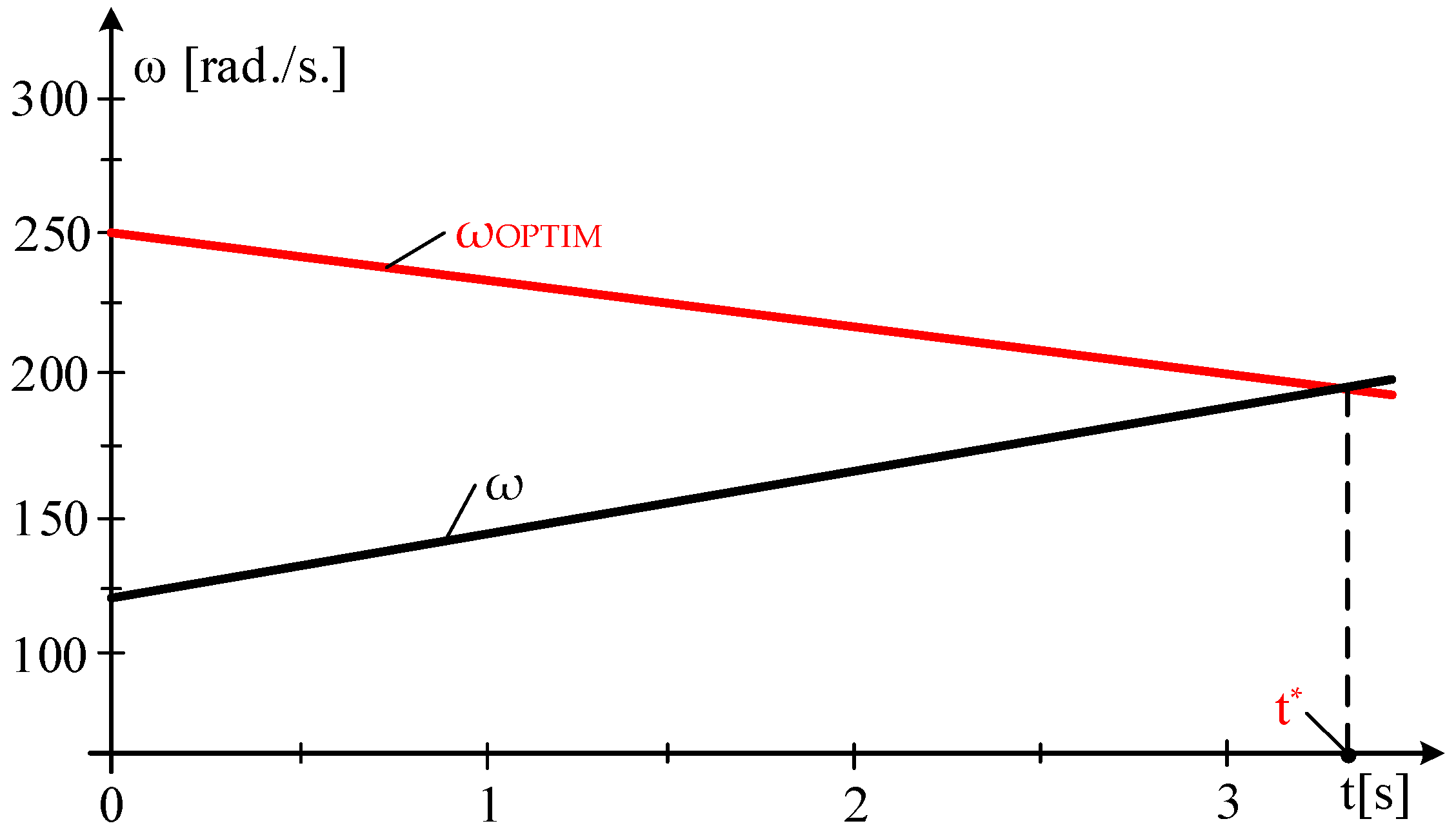
3.1. Achieving the Maximum Power Point of the Wind Turbine System

Achieving the maximum power point of the turbine necessitates an acceleration towards the optimal operating condition. This can be achieved in the shortest time possible through two methods:
  • Disconnection of the generator from the network (a slower method).
  • Converting the generator to operate in motor mode (a faster method).
The EG is viewed as to be decoupled from the grid and possesses the MAS value ω(0) = 122 [rad/s]. Based on the equation that describes powers of form:
J d ω d t ω = P W T ω , t
it is obtained:
511.92 d ω d t ω = 650860 10.47 0.73171 t ω 1.7488 10 2 e 41.495 10.47 0.73171 t ω 10.47 0.73171 t 3 ω 0 = 122
By solving it, we obtain the time variation of the mechanical angular speed, ω.
At the time t*, according to Figure 3, the angular velocity MAS ω is measured at ω(3.3) = 197.6 [rad/s], which represents approximately equal to the optimal MAS:
ω O P T I M V = 24.046 10.47 0.73171 t = 24.046 10.47 0.73171 3.3 = 197.67   [ rad / s ]
At t = 3.3 s, the values of the optimal, ωOPTIM, and real mechanical angular velocities, ω, are equal, the system functions at the turbine’s maximum power point, t*.
At the specific time t*, the speed of wind is measured at:
V 3.3 = + 8.13 10.47 3.433 3.33 = 8.2207   [ m / s ]
Based on, PWT(V,ω), the the power characteristic at ω(3.3):
P W T = 650860 8.2207 ω 1.7488 10 2 e 41.495 8.2207 ω 8.2207 3 ω = 197.67
the power generated by the WT is obtained at a value of:
P W T 8.2207 = 1.5516 10 6   [ W ]

3.2. Sustaining the Wind System at the Turbine’s Maximum Power Point

From the power equation, when operating in MPP, the electromagnetic power, PEG, is derived at the shaft of the EG:
J d ω d t ω = P W T P E G
In the energetically optimal zone, when operating at MPP, the optimal mechanical angular speed, ωOPTIM, is determined by the wind speed, expressed as: ωOPTIM = 24.046·V.
In the optimal range, the current MAS, ω, must equal the optimal mechanical angular velocity, ωOPTIM, such that ω = ωOPTIM. Consequently, the power equation is expressed as follows:
J d ω O P T I M d t ω O P T I M = P W T M A X P E G O P T I M
or:
24.046 J d V d t 24.046 V = P W T M A X P E G O P T I M
Therefore, by understanding how the optimal speed is influenced by wind speed, we can ascertain the optimal power output of the electric generator:
P E G O P T I M = P W T M A X 24.046 2 J d V d t V
The optimal electromagnetic power is achieved at an equivalent moment of inertia of J = 511.92 [kg·m2]:
P E G O P T I M = P W T M A X 24.046 2 511.92 d V d t V
Subsequently, at PWT-MAX = 2792.8·V3, it follows that:
P E G O P T I M = 2792.8 V 3 2.96 10 5 d V d t V
After the WT has been brought into the MPP at the time t*, the EG connects to the grid and charges at the power level:
P E G = P W T J d ω O P T I M d t ω O P T I M = P W T 2.96 10 5 d V d t V
The power of WT, P*WT can be determined by two methods:
  • With MM-WT:
P W T M A X = k p V 3 = 2792.8 V 3
  • By integrating the kinetic momentum equation multiplied with ω, we derive the kinetic energies:
J ω k 2 ω k 1 2 2 = t k 1 t k P W T d t t k 1 t k P E G d t
A temporal linear variation of the PWT and PEG powers, yields:
J ω k 2 ω k 1 2 2 = P W T t k 1 + P W T t k 2 Δ t P E G t k 1 + P E G t k 2 Δ t
or:
J ω k 2 ω k 1 2 2 Δ t = P W T t k 1 + P W T t k 2 P E G t k 1 + P E G t k 2
where: ωkMAS at tk moment, ω(k−1)MAS at t(k−1), Δt = tkt(k−1), PWT(tk−1), PEG(tk−1)—powers at WT and EG at the time tk−1, PWT(tk), PEG(tk)—powers at the moment tk.
Consequently, the average power output from the WT is obtained over the specified period tk−1 − tk:
P W T A V E R A G E t k = J ω k 2 ω k 1 2 2 Δ t + P E G A V E R A G E t k
where:
t k = t k + t k 1 2
The duration of the time interval Δt is a value that must be correlated with the derivative of wind speed, dV/dt, and J, the equivalent inertia moment.

3.2.1. Sample Interval Value

The sampling interval value should be comparable to the value of the electromechanical time constant, H. In this particular case, it is as follows:
  • J = 511.92 [kg·m2]—equivalent moment of inertia.
  • PN = 2.5 [MW] = 2,500,000 [W]—rated power.
  • ωN = 157.08 [rad/s]—nominal mechanical angular speed.
  • H-value:
H = J ω 2 2 P N = 511.92 157.08 2 5000000 = 2.5262   [ s ]
Therefore, a sampling interval of Δt = 1 [s] is deemed valid, as Δt = 1 [s] exceeds H = 2.5262 [s].
In the examined location, the fluctuation of wind speed is particularly significant during the summer months. However, the duration of these wind speed variations falls within the magnitude of the sampling interval Δt and the time constant of the electromechanical system, H.
The power values at EG, PEG(tk−1), and PEG(tk) corresponding to MAS ωk−1 and ωk at the time points tk−1 and tk are achieved with minimal inaccuracies via direct measurements, thus ensuring their validity. These values are then used to calculate the average power from the wind turbine (WT) over the time interval Δt = tktk−1 = 1.
P W T K I N E T I C = J ω k 2 ω k 1 2 2 Δ t = 511.92 ω k 2 ω k 1 2 2   [ rad / s ]
The maintenance of the WT in the MPP is carried out in accordance with the proposed adjustment algorithm outlined below.

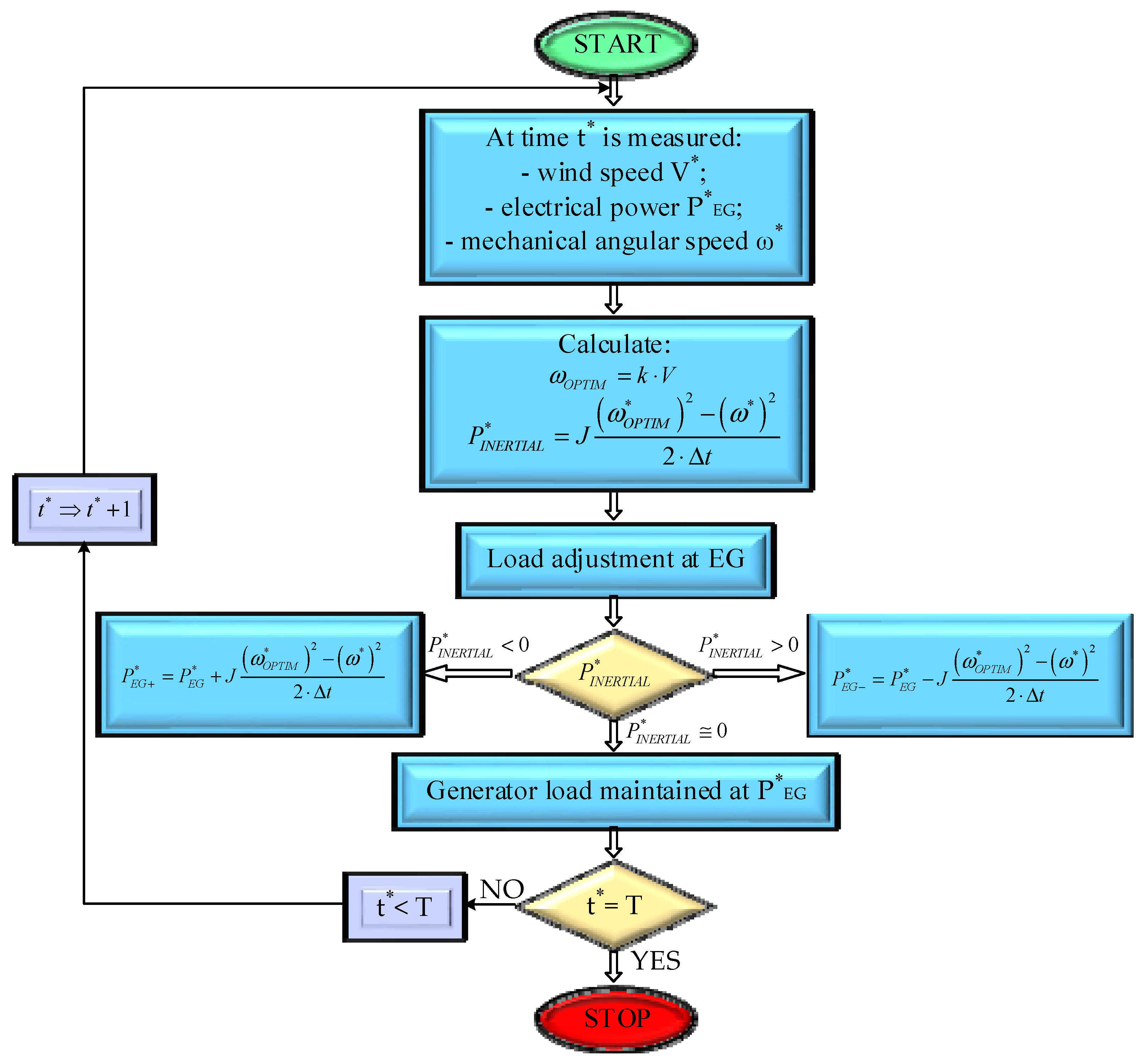
3.2.2. Control Algorithm

The algorithm consists of three operational steps (Figure 4):
  • Step 1—the following are measured: wind speed, V*, generator power P*EG and speed, ω*;
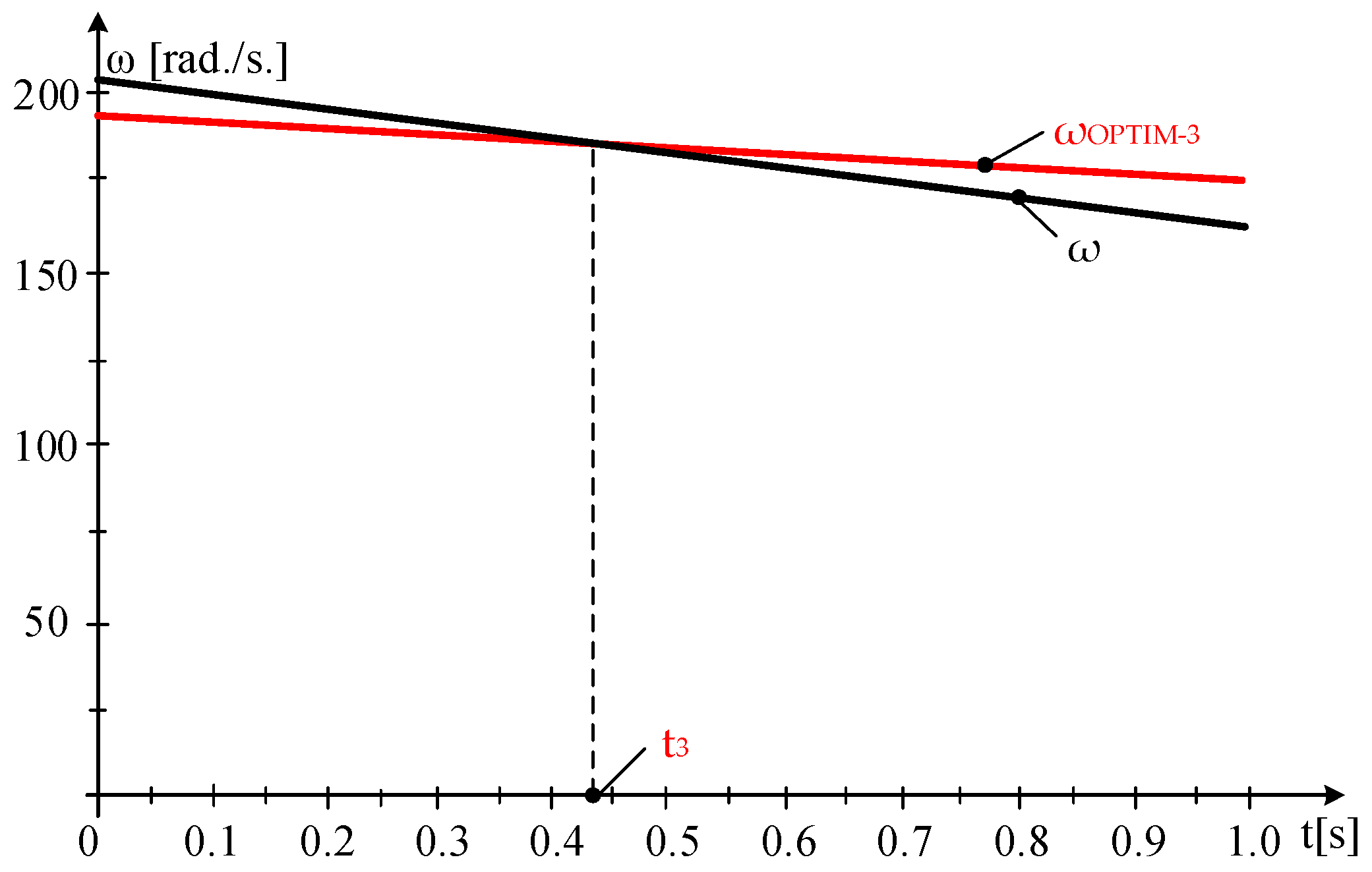
  • Step 2—the optimal mechanical angular velocity, ω*OPTIM, is calculated using the formula ω*OPTIM = kPV*, along with the inertial power.
P I N E R T I A L = J ω O P T I M 2 ω 2 2 Δ t
  • Step 3—The loading at EG is adjusted according to the sign of the inertial power value, P*INERTIAL, as follows:
  • P*INERTIAL < 0, results in an increase in the EG load raised to the power of:
P E G + = P E G + J ω O P T I M 2 ω 2 2 Δ t
2.
P*INERTIAL > 0, the load on EG decreases at the rate of:
P E G = P E G J ω O P T I M 2 ω 2 2 Δ t
3.
P*INERTIAL > 0, the EG load is maintained at the P*EG power level.
The system control is executed over a time interval T, with a sampling step that depends on dV/dt, the wind speed derivative and J, the equivalent inertia moment. At a sampling interval of 1 s, three operational steps are completed.
Simulation is utilized to verify the MPP and to determine the precise moments at which power imbalances take place.

3.2.3. Time Intervals in Which Power Gaps Occur

From the analysis of the actual variation in wind speed, as in Figure 2, it is evident that there are intervals characterized by an increase in wind velocity and others when it decreases. When functioning inside the MPP region, the optimal power output of the electric generator, referred to as PEG-OPTIM, will fluctuate in response to the wind, potentially leading to intervals where power deficits occur.
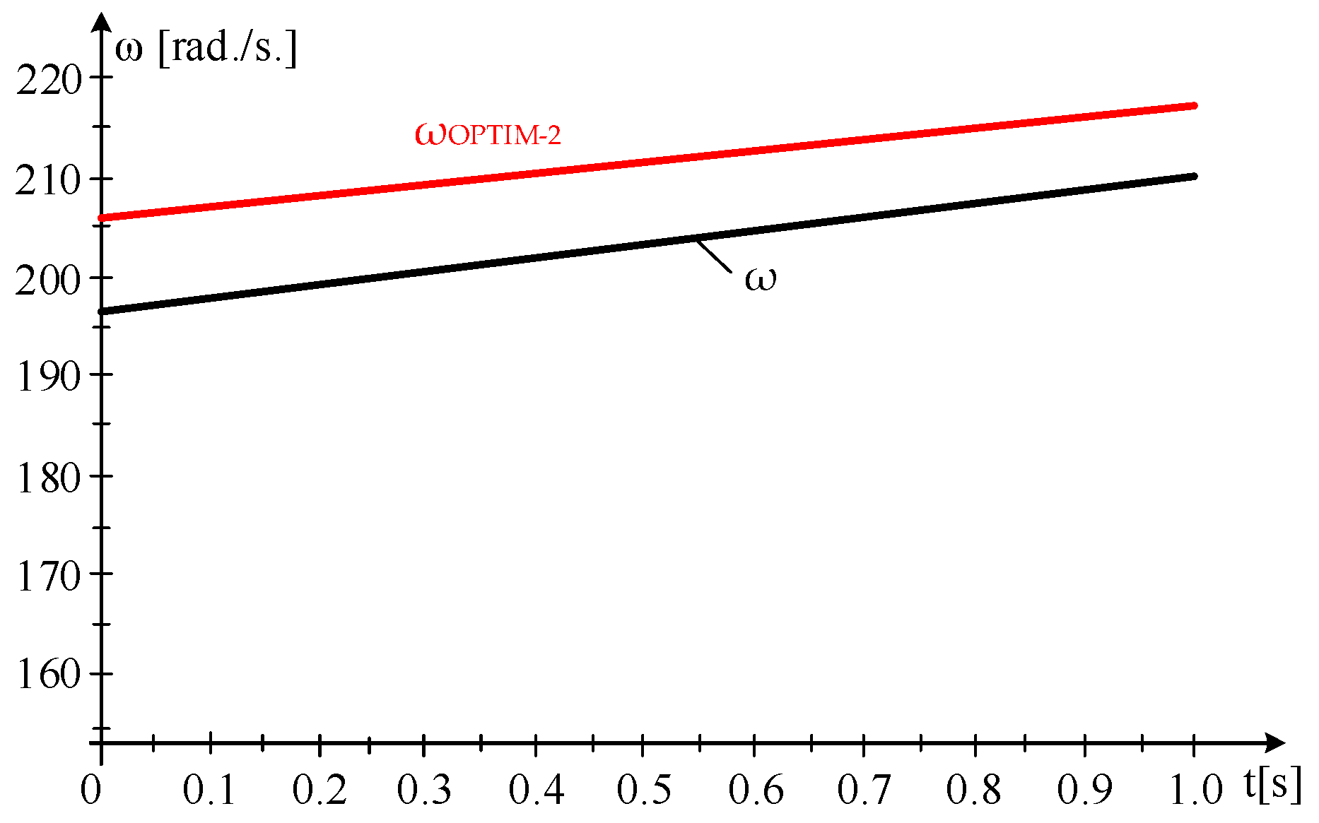
  • Case Study 2—Verification in the MPP Area
The system’s performance is assessed after it attains the turbine’s maximum power point. At time t*, the wind turbine (WT) functions at the maximum power point, designated as point B, as in Figure 2 and reflected in Table 2.
At t* = 0, the system functions in state B, at the maximum power point of the turbine, where the optimal mechanical angular velocity, ωOPTIM, equals to the actual angular speed, ω:
ω O P T I M = ω = 24.046 8.13 = 195.49   [ rad / s ]
The wind speed being V* = 8.13 [m/s], the load of EG is at P*EG of value:
P E G 0 = P W T M A X = k P V 3 = 2792.8 8.13 3 = 1.5008 10 6   [ W ]
On the interval B-C, considering the variation of wind speed to a linear progression, it follows:
V B C t = 8.13 + 9.52 8.13 6.631 3.433 t
The captured wind energy, EWIND, can be determined by integrating the power of the WT:
E W I N D = P W T d t
or:
E W I N D d t = P W T
The interval B-C is divided into four distinct subintervals:
  • Subinterval 1:
Given that the sampling period is 1 s, at t* = 1 s, the obtained wind speed results:
V 1 = 8.13 + 9.52 8.13 6.631 3.433 1 = 8.5646   [ m / s ]
The variation of the wind speed is linear, between 8.13 [m/s] and 8.5646 [m/s].
V B C 1 t = 8.13 + ( 8.5646 8.13 ) t = 0.4346 t + 8.13
The optimal MAS, ωOPTIM, is:
ω O P T I M 1 = 24.046 0.4346 t + 8.13
For these values, the energy and motion equations are derived in:
511.92 d ω d t ω = 650860 0.4346 t + 8.13 ω 1.7488 10 2 e 41.495 0.4346 t + 8.13 ω 0.4346 t + 8.13 3 1.5008 10 6 d E d t = 650860 0.4346 t + 8.13 ω 1.7488 10 2 e 41.495 0.4346 t + 8.13 ω 0.4346 t + 8.13 3 ω 0 = 195.49 E 0 = 0
In one second, significant wind energy is collected:
E W I N D 1 = E 1 = 1.6236 10 6   [ J ]
At maximum power output, the captured wind energy during the same period is valued at:
E W I N D M A X 1 = 0 1 P W T M A X d t = 0 1 2792.8 0.4346 t + 8.13 3 d t = 1.6254 10 6   [ J ]
During the same period, the amount of electrical energy delivered is:
E E L E C T R I C A L 1 = 0 1 P E G d t = 1.5008 10 6   [ J ]
At time t* = 1 s, as Figure 5 illustrates, the MAS ω is measured at ω(1) = 196.71 rad/s, in comparison with the optimal MAS.
ω O P T I M 1 = 24.046 8.5646 = 205.94   [ rad / s ]
Due to the fact that ωOPTIM-1 is greater than ω(1), ωOPTIM-1 > ω(1), the turbines MPP was not attained at t* = 1 [s].
The value of inertial power being positive, P*INERTIAL > 0:
P I N E R T I A L 1 = J ω O P T I M 2 ω 2 2 Δ t = 511.92 205.94 2 196.71 2 2 = 9.5126 10 5   [ W ]
Within subinterval 2, the load of EG decreases at the rate of:
P E G 2 = P E G J ω O P T I M 2 ω 2 2 Δ t = 1.5008 10 6 9.5126 10 5 = 5.4954 10 5   [ W ]
  • Subinterval 2
At t = 2 [s], the value of the wind speed is:
V 2 = 8.13 + 9.52 8.13 6.631 3.433 2 = 8.9993   [ W ]
Within the subinterval 2, the wind speed has a straight variation ranging between 8.5646 [m/s] and 8.9993 [m/s]:
V B C 2 t = 8.5646 + ( 8.9993 8.5646 ) t = 0.4347 t + 8.5646
MAS optim, ωOPTIM, is:
ω O P T I M 2 = 24.046 0.4347 t + 8.5646   [ rad / s ]
When comparing subinterval 2 to subinterval 1, there is a 1-s shift in the origin of time. This pattern continues to recur in each subsequent analyzed subinterval.
The energy and motion equations are expressed as follows:
511.92 d ω d t ω = 650860 0.4347 t + 8.5646 ω 1.7488 10 2 e 41.495 0.4347 t + 8.5646 ω 0.4347 t + 8.5646 3 5.4954 10 5 d E d t = 650860 0.4346 t + 8.5646 ω 1.7488 10 2 e 41.495 0.4346 t + 8.5646 ω 0.4346 t + 8.5646 3 ω 0 = 196.71 E 0 = 0
The wind energy harnessed within a single second is valued at:
E W I N D 1 = E 1 = 1.8883 10 6   [ J ]
When operating in MPP, the captured wind energy is:
E W I N D M A X 1 = 0 1 P W T M A X d t = 0 1 2792.8 0.4346 t + 8.5646 3 d t = 1.8927 10 6   [ J ]
The supplied electrical energy is:
E E L E C T R I C A L 1 = 0 1 P E G d t = 5.4954 10 5   [ J ]
At t* = 1 [s], the mechanical angular speed ω is measured at ω(1) = 209.58 [rad/s]. In contrast, the optimal mechanical angular speed is calculated as ωOPTIM-2 = 24.046⋅8.9993 = 216.4 [rad/s], as illustrated in Figure 6.
Once that ωOPTIM-2 is greater than ω(1), the turbine did not achieve its maximum power point at t* = 1 [s]. Given that P*INERTIAL > 0, the inertial power is positive,
P I N E R T I A L 1 = J ω O P T I M 2 ω 2 2 Δ t = 511.92 216.4 2 209.58 2 2 = 7.4361 10 5   [ W ]
the loading of EG should diminish within subinterval 3, reaching the following:
P E G 3 = P E G J ω O P T I M 2 ω 2 2 Δ t = 5.4954 10 5 7.4361 10 5 = 1.9407 10 5 < 0
The negative value of power at EG necessitates a transition to motor mode.
For the mechanical angular speed, ω, to attain its optimum, ωOPTIM, within subinterval 3, it is essential for EG to be operated in motor mode, a condition that is challenging to achieve in practice.
  • Subinterval 3
The EG power is less than zero within the interval 3, leading to its discharge, thus P**EG-3 = 0. For t = 3 [s], the wind is:
V 3 = 8.13 + 9.52 8.13 6.631 3.433 3 = 9.4339   [ W ]
Within the interval of 3, the wind velocity decreases linear, starting with 8.9993 [m/s] until 8.4339 [m/s].
V B C 3 t = 8.9993 + ( 9.4339 8.9993 ) t = 0.4346 t + 8.9993
ωOPTIM, is:
ω O P T I M 3 = 24.046 0.4346 t + 8.9993   [ rad / s ]
Consequently, the governing differential equations system related to energy and motion is expressed as follows:
511.92 d ω d t ω = 650860 0.4346 t + 8.9993 ω 1.7488 10 2 e 41.495 0.4346 t + 8.9993 ω 0.4346 t + 8.9993 3 d E d t = 650860 0.4346 t + 8.9993 ω 1.7488 10 2 e 41.495 0.4346 t + 8.9993 ω 0.4346 t + 8.9993 3 ω 0 = 209.58 E 0 = 0
The value of wind energy captured in one second is:
E W I N D 1 = E 1 = 2.1869 10 6   [ J ]
In the context of MPP operation, the value of the captured wind energy during the same period is:
E W I N D M A X 1 = 0 1 P W T M A X d t = 0 1 2792.8 0.4346 t + 8.9993 3 d t = 2.1877 10 6   [ J ]
The amount of electricity debited is zero:
E E L E C T R I C A L 1 = 0
At t* = 1 [s], ω, the MAS, is ω(1) = 229.06 [rad/s], which exceeds the optimal MAS:
ω O P T I M 3 = 24.046 9.4339 = 226.85   [ rad / s ]
At t3, as illustrated in Figure 7, the mechanical angular velocity ω attained its optimal value.
Thus, the accuracy of the proposed control algorithm has been confirmed. At this moment, the WT is operating at its MPP with the optimal MAS.
The value of harnessed wind energy is reflected in the electrical energy supplied to the power grid as well as in the kinetic energy associated with the masses in rotation. The kinetic energies of the subintervals—three in number, are:
Δ E K I N E T I C 1 = J ω 1 2 ω 0 2 2 = 511.92 196.71 2 195.49 2 2 = 1.2247 10 5   [ J ]
Δ E K I N E T I C 2 = J ω 1 2 ω 0 2 2 = 511.92 209.58 2 196.71 2 2 = 1.3384 10 6   [ J ]
Δ E K I N E T I C 3 = J ω 1 2 ω 0 2 2 = 511.92 229.58 2 209.58 2 2 = 2.1871 10 6   [ J ]
In conclusion, the energies across the three subintervals are displayed in Table 2, while the evolutions are illustrated in Figure 8.

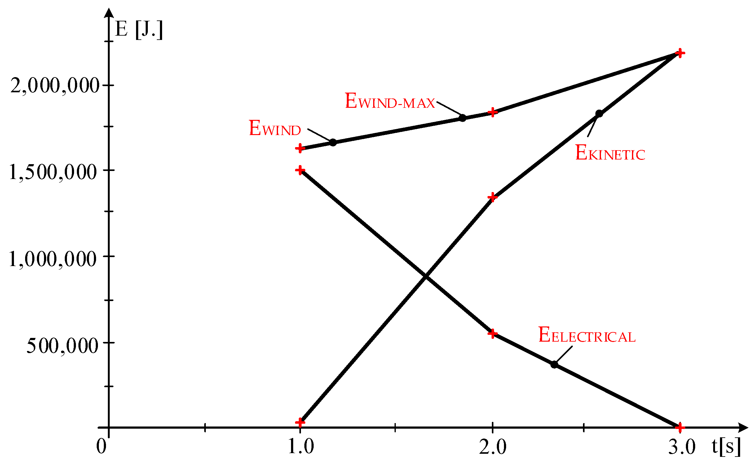
3.2.4. Energy Balance

The energy balance confirms that EWIND, the wind energy captured, is present in the generated electrical energy, EELECTRICAL, and in the kinetic energy associated with rotating masses, ΔEKINETIC.
The energy balance within subinterval 1, EWIND = 1.6236·106 [J], lie in:
E E L E C T R I C A L + Δ E K I N E T I C = 1.5008 10 6 + 1.2247 10 5 = 1.6233 10 6   [ J ]
The energy balance within subinterval 2, EWIND = 1.8883·106 [J] lie in:
E E L E C T R I C A L + Δ E K I N E T I C = 5.4954 10 5 + 1.3384 10 6 = 1.8879 10 6   [ J ]
The energy balance within subinterval 3, EWIND = 2.1869·106 [J] lie in:
E E L E C T R I C A L + Δ E K I N E T I C = 0 + 2.1871 10 6 = 2.1871 10 6   [ J ]
At time t3, maximum wind energy is collected, also while the energy generator is discharging (P**EG-3 = 0). The turbine functions in MPP at the optimal MAS, energy that is not flowed into the system, (P**EG-3 is zero), but can be located in the kinetic energy of the rotating masses. It appears that the turbine is not operating within the optimal energy efficiency range. There is a power gap at this point in time, it poses a disadvantage to the energy system stability.
From the variations in energies values (Figure 8), follows that:
  • The values of the produced electrical energies, EELECTRICAL, decrease (the power to the generator diminishes).
  • The variations of the kinetic energies, ΔEKINETIC, increase and compensate for the reduction of grid-injected electrical energies.
  • The harnessed wind energy increases in direct proportion to the increase in wind speed.
In conclusion, during periods where the wind speed grows, power gaps can occur if dV/dt, the wind speed derivative, and J, the equivalent inertia moment, surpass specific thresholds.

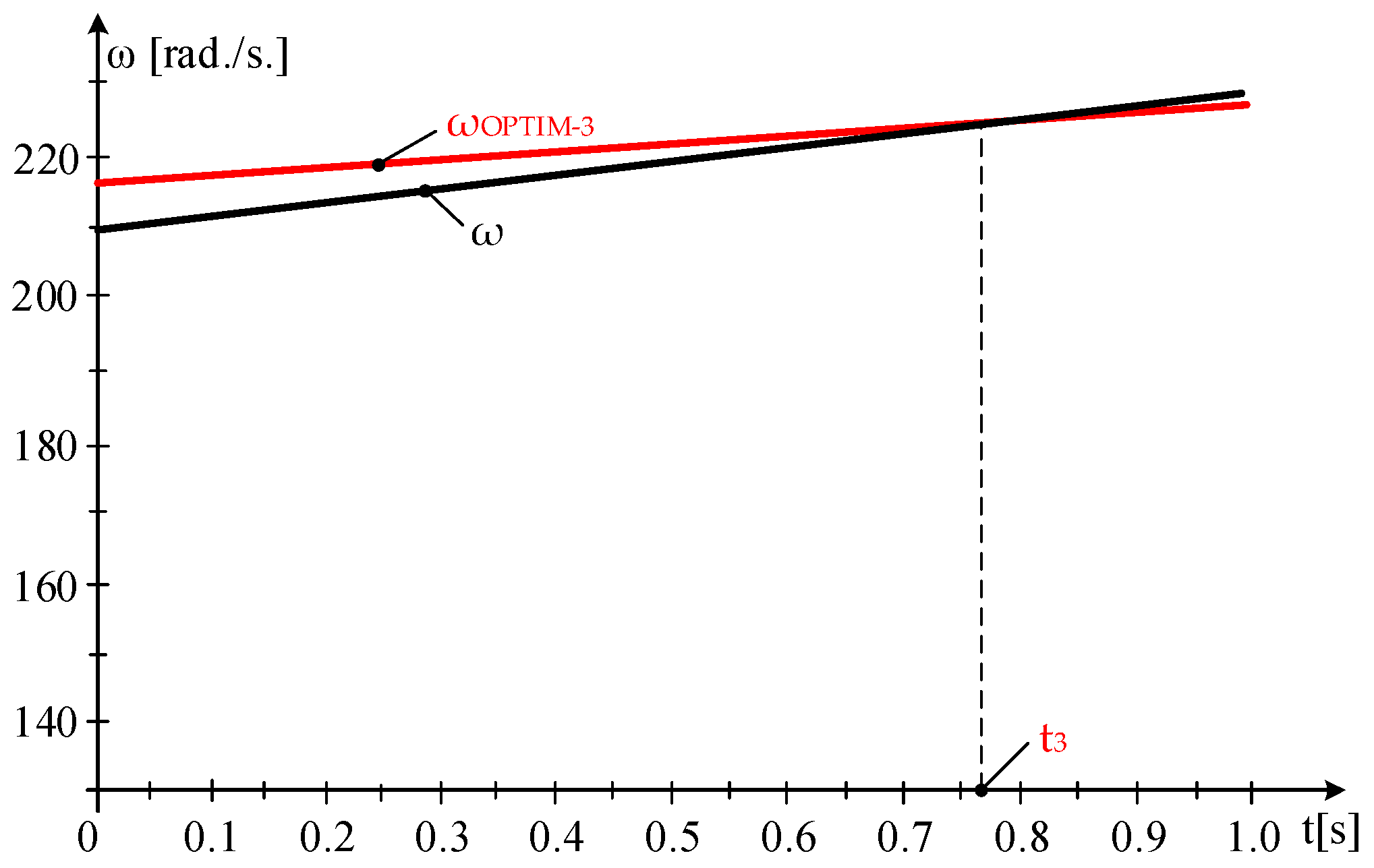
3.2.5. Periods Characterized by Diminished Wind Speed

  • Case Study 3—MPP Region Characterized by Diminishing Wind Velocity
In Figure 9, we select the time interval D-E. during which the wind speed diminishes. The corresponding time intervals and the related speeds are detailed in Table 3.
At point D, Figure 9, WT is assumed to operate in MPP at the equality of the values of the optimal MAS, ωOPTIM and the real angular velocities, ω:
ω O P T I M D = ω D = 24.046 9.52 = 228.92   [ rad / s ]
The velocity of the wind being VD = 9.52 [m/s], the EG load is at the PEG-D power of value:
P E G D = P W T M A X = k P V 3 = 2792.8 9.52 3 = 2.4096 10 6   [ W ]
Taking into consideration the linear variation in wind speed over the D-E interval, it follows:
V D E t = 9.52 + 7.145 9.52 43.073 39.858 t = 9.52 0.73872 t
The interval D-E is divided into three subintervals.
  • Subinterval 1:
Given that the sampling period is 1 s, at t* = 1 s, the calculated wind is:
V 1 = 9.52 + 7.145 9.52 43.073 39.858 1 = 8.7813   [ m / s ]
The wind speed exhibits a linear decrease ranging between 9.52 [m/s] and 8.7813 [m/s]:
V D E 1 t = 9.52 + 8.7813 9.52 t = 9.52 0.7387 t
The optimal mechanical angular speed, ωOPTIM, is:
ω O P T I M 1 = 24.046 9.52 0.7387 t   [ rad / s ]
Thus, the energy and motion equations are derived in the following:
511.92 d ω d t ω = 650860 9.52 0.7387 t ω 1.7488 10 2 e 41.495 9.52 0.7387 t ω 9.52 0.7387 t 3 2.4096 10 6 d E d t = 650860 9.52 0.7387 t ω 1.7488 10 2 e 41.495 9.52 0.7387 t ω 9.52 0.7387 t 3 ω 0 = 228.92 E 0 = 0
The amount of wind energy harnessed in a single second is EWIND(1) = 2.1382·106 [J]. At maximum power operation, the harnessed wind energy within the same time frame is valued at:
E W I N D M A X 1 = 0 1 P W T M A X d t = 0 1 2792.8 9.50 + 0.7387 t 3 d t = 2.1434 10 6   [ J ]
During the same time frame, the debited electricity is:
E E L E C T R I C A L 1 = 0 1 P E G d t = 2.4096 10 6   [ J ]
At t* = 1 [s], as highlighted in Figure 10, ω, the MAS is ω(1) = 226.59 [rad/s] compared with the optimal MAS:
ω O P T I M 1 = 24.046 8.7813 = 211.16   [ rad / s ]
Since ωOPTIM-1 is less than ω(1), the value of the inertial power is negative, indicating that P*INERTIAL is less than 0:
P I N E R T I A L 1 = J ω O P T I M 2 ω 2 2 Δ t = 511.92 211.16 2 226.59 2 2 = 1.7289 10 6   [ W ]
The loading of the EG increases within subinterval 2, at the power of:
P E G 2 = P E G J ω O P T I M 2 ω 2 2 Δ t = 2.4096 10 6 + 1.7289 10 6 = 4.1385 10 6
  • Subinterval 2
At t = 2 [s], the wind speed is:
V 2 = 9.52 + 8.7813 9.52 2 = 8.0426   [ m / s ]
exhibiting a linear change, ranging between 8.7813 [m/s] and 8.0426 [m/s].
V D E 2 t = 8.7813 + 8.0426 8.7813 t = 8.7813 0.7387 t
The optimal MAS, ωOPTIM, is:
ω O P T I M 1 = 24.046 8.7813 0.7387 t   [ rad / s ]
The energy and motion equations result in:
511.92 d ω d t ω = 650860 8.7813 1.7387 t ω 1.7488 10 2 e 41.495 8.7813 0.7387 t ω 8.7813 0.7387 t 3 4.1385 10 6 d E d t = 650860 8.7813 0.7387 t ω 1.7488 10 2 e 41.495 8.7813 0.7387 t ω 8.7813 0.7387 t 3 ω 0 = 226.59 E 0 = 0
In a single second, the harnessed energy from the wind is valued at:
E W I N D 1 = E 1 = 1.6549 10 6   [ J ]
At operation at the MPP, the captured wind energy during the same period, is:
E W I N D M A X 1 = 0 1 P W T M A X d t = 0 1 2792.8 8.7813 0.7387 t 3 d t = 1.6656 10 6   [ J ]
For the same period, the generated electrical energy is:
E E L E C T R I C A L 1 = 0 1 P E G d t = 4.1385 10 6   [ J ]
At t* = 1 [s], ω, the MAS is ω(1) = 204.06 [rad/s], compared to the optimal MAS:
ω O P T I M 2 = 24.046 8.0426 = 193.39   [ rad / s ]
Since ωOPTIM-1 is less than ω(1), the inertial power is negative, indicating that P*INERTIAL < 0:
P I N E R T I A L 1 = J ω O P T I M 2 ω 2 2 Δ t = 511.92 193.39 2 204.06 2 2 = 1.0855 10 6   [ W ]
on subinterval 3, the load on EG is increased to the power of:
P E G 2 = P E G J ω O P T I M 2 ω 2 2 Δ t = 4.1385 10 6 + 1.0855 10 6 = 5.224 10 6   [ W ]
  • Subinterval 3
The wind speed is at t = 3 [s]:
V 3 = 9.52 + 8.7813 9.52 3 = 7.3039   [ m / s ]
Wind speed decreases from 8.0426 [m/s] to 7.3039 [m/s]:
V D E 3 t = 8.0426 + 7.3039 8.0426 t = 8.0426 0.7387 t
ωOPTIM, the optimal MAS, is:
ω O P T I M 3 = 24.046 8.0426 0.7387 t   [ rad / s ]
For the values provided, the energy and motion equations become:
511.92 d ω d t ω = 650860 8.0426 0.7387 t ω 1.7488 10 2 e 41.495 8.0426 0.7387 t ω 8.0426 0.7387 t 3 5.224 10 6 d E d t = 650860 8.0426 0.7387 t ω 1.7488 10 2 e 41.495 8.0426 0.7387 t ω 8.0426 0.7387 t 3 ω 0 = 204.06 E 0 = 0
In a duration of one second, the wind energy captured is EWIND(1) = E(1) = 1.2619·106 [J]. At maximum power point operation, the harnessed wind energy within the same period is:
E W I N D M A X 1 = 0 1 P W T M A X d t = 0 1 2792.8 8.0426 0.7387 t 3 d t = 1.2647 10 6   [ J ]
The delivered electricity for the same period is:
E E L E C T R I C A L 1 = 0 1 P E G d t = 5.224 10 6   [ J ]
At t* = 1 [s], ω, the MAS is measured as ω(1) = 161.74 [rad/s], compared to the optimal MAS:
ω O P T I M 3 = 24.046 7.3039 = 175.63   [ rad / s ]
At time t3, as Figure 11 highlights, the optimal MAS, ωOPTIM-3, is equivalent to ω, the MAS, indicating that the MPP was attained. Consequently, the control algorithm has been validated.
Since ωOPTIM-3 > ω(1), the value of the inertial power is positive, P*INERTIAL > 0:
P I N E R T I A L 1 = J ω O P T I M 2 ω 2 2 Δ t = 511.92 175.63 2 161.74 2 2 = 1.1994 10 6   [ W ]
In the given context, during the subsequent time interval, the EG charge should decrease to the power:
P E G 2 = P E G J ω O P T I M 2 ω 2 2 Δ t = 5.224 10 6 1.1994 10 6 = 4.0246 10 6   [ W ]
The harnessed wind energy is reflected in the electricity provided to the grid as well as in the kinetic energy associated with the rotating components. The fluctuations in kinetic energy across the three subintervals are as follows:
Δ E K I N E T I C 1 = J ω 1 2 ω 0 2 2 = 511.92 226.59 2 228.92 2 2 = 2.7166 10 5   [ J ]
Δ E K I N E T I C 2 = J ω 1 2 ω 0 2 2 = 511.92 204.06 2 226.59 2 2 = 2.4835 10 6   [ J ]
Δ E K I N E T I C 3 = J ω 1 2 ω 0 2 2 = 511.92 161.74 2 204.58 06 2 2 = 3.9624 10 6   [ J ]
In conclusion, the values of the energy for the three subintervals are synthesized in Table 4.
Over a 3 s interval, where the wind speed decreases, 7.145 [m/s] < V(t) < 9.52 [m/s], Figure 12 represents the energy evolutions.
In this scenario, the energy balance is EWIND = EELECTRICAL + ΔEKINETIC. Across the three subintervals, it follows that: ω*OPTIM = k·V*.
  • Subinterval 1:
2.1382 10 6 = 2.4096 10 6 2.7166 10 5 = 2.1379 10 6   [ J ]
  • Subinterval 2:
1.6549 10 6 = 4.1385 10 6 2.4835 10 6 = 1.655 10 6   [ J ]
  • Subinterval 3:
1.2619 10 6 = 5.224 10 6 3.9624 10 6 = 1.2616 10 6   [ J ]
On the periods during which the wind velocity diminishes, power gaps are absent, although the MAS velocity ω leans towards the value of the optimal MAS, ωOPTIM. The turbine functions within MPP at the optimal MAS. The output power in the grid (PEG) exceeds the WT provided power, excepting the kinetic energy of the rotating masses. This situation presents a benefit for the purpose of maintaining stability within the energy system.
From the energy variations illustrated in Figure 12, it can be concluded that:
  • The values of electrical energy output, EELECTRICAL, increase even as wind speed decreases.
  • The absolute differences in the values of the ΔEKINETIC kinetic energies, grow and counterbalance the decline in the values of the captured wind energies.
  • The values of the harnessed wind energies diminish in direct proportion to the reduction in wind speed.
In conclusion, during the periods when the wind velocity decreases, there are no power gaps, regardless of the values of the wind speed derivative, dV/dt, and J, the inertia equivalent moment.

4. Discussion

As a result of the presented study, the following findings were obtained:
  • MM-WT was deduced, with experimental data.
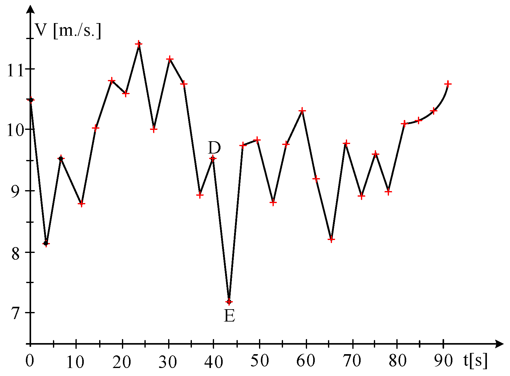
  • The actual wind speed variation in the Dobrogea region was analyzed, and the motion equation was employed to visualize its operation within the optimal area.
  • A method has been proposed to bring and maintain the turbine in its MPP.
  • A control algorithm has been validated, which is based on the sign of the inertial power value, derived from experimental data including wind speed and mechanical angular speed.
  • The time intervals in which power gaps occur have been analyzed.
  • The periods during which wind speed diminishes were analyzed.
Based on the obtained results, the following key points can be emphasized:
  • The system is brought to the turbines MPP in the shortest possible time by either disconnecting the generator from the grid or by switching the engine to motor mode.
  • By calculating the disparity between optimal MAS and present MAS, one can prescribe the power output of the generator.
  • When the wind speed increases, gaps of power occur, leading to the disconnection of the generator from the grid, particularly when it is necessary to operate within the optimal energy efficiency range.
  • As wind speeds diminish over time, power gaps do not occur; however, it is essential to function at MPP. The electrical power output in the system is higher than the power output of the turbine, with the excess power generated from the varying kinetic energies of the rotating masses.
The proposed method establishes a framework for control that considers wind and the angular mechanical speed. Based on the determination of the variations in kinetic energy of rotating masses, values acquired through measurements, the system is optimized to reach its MPP.
The proposed approach addresses genuine needs for wind farms located in areas where wind speed fluctuates significantly over time.
The practical advantages of the proposed approach enable the extraction of maxi-mum wind energy at considerably fluctuating wind velocities over time, where mechanical inertia and fluctuations in wind velocity play a crucial role.

5. Conclusions

This study examines the performance of a WT under fluctuating wind speeds over time and develops a control system based upon the fluctuations of kinetic energies of rotating masses, which are influenced by the wind speed values. In instances of significant changes in wind speed, the set value at the generator may become negative, leading to a power deficit within the electrical energy system.

Author Contributions

Conceptualization, C.P.C. and E.S.; Methodology, C.P.C. and S.C.; Software, C.P.C. and S.C.; Validation, C.P.C., S.C., and E.S.; Formal analysis, E.S.; Investigation, C.P.C. and S.C.; Resources, E.S.; Data curation, C.P.C.; Writing—original draft preparation, C.P.C.; Writing—review and editing, E.S.; Visualization, S.C. and E.S.; Supervision, C.P.C.; Project administration, C.P.C. and E.S.; Funding acquisition, C.P.C. All authors have read and agreed to the published version of the manuscript.

Funding

This research received no external funding.

Data Availability Statement

The original contributions presented in the study are included in the article, further inquiries can be directed to the corresponding author.

Conflicts of Interest

The authors declare no conflicts of interest. The funders had no role in the design of the study; in the collection, analyses, or interpretation of data; in the writing of the manuscript; or in the decision to publish the results.

Abbreviations

The following abbreviations are utilized:
WTwind turbine
MPPmaximum power point
MASmechanical angular speed
EGelectric generator
DFIGdouble fed induction generator
PODpower oscillation damping
MMmathematical model
Jequivalent inertia moment
Vwind speed
MWTmoment related to the shaft of the electric generator
MEGelectromagnetic torque at the electric generator
PNrated power
PWTWT power relative to the electric generator shaft
PWT-AVERAGEaverage power value from the wind turbine
PEGpower of the electric generator
PINERTIALinertial power
Helectromechanical time constant
ωmechanical angular speed
ωNnominal mechanical angular speed
ωOPTIMoptimum angular speed
ωMAXIMmaximum angular speed
ωREALreal angular speed
nOPTIMoptimum speed
Cp(λ)power conversion coefficient
ρair density in the operating location
Rpradius blades
EWINDwind energy
EELECTRICALelectrical energy delivered
ΔEKINETICkinetic energy of the rotating masses

References

  1. Wind. Available online: https://www.iea.org/energy-system/renewables/wind (accessed on 19 March 2025).
  2. Sachin, G.; Shree, K.M.; Shivam, K.; Deepesh, A. A Consolidation Review of Major Wind Turbine Models in Global Market. In Proceedings of the 2020 International Conference on Power Electronics & IoT Applications in Renewable Energy and its Control (PARC), Mathura, India, 28–29 February 2020. [Google Scholar]
  3. Ketian, L.; Zhengxi, C.; Xiang, L.; Yi, G. Analysis and Control Parameters Optimization of Wind Turbines Participating in Power System Primary Frequency Regulation with the Consideration of Secondary Frequency Drop. Energies 2025, 18, 1317. [Google Scholar] [CrossRef]
  4. Rebello, E.; Watson, D.; Rodgers, M. Performance Analysis of a 10 MW Wind Farm in Providing Secondary Frequency Regulation: Experimental Aspects. IEEE Trans. Power Syst. 2019, 34, 3090–3097. [Google Scholar] [CrossRef]
  5. Huynh, P.; Tungare, S.; Banerjee, A. Maximum Power Point Tracking for Wind Turbine Using Integrated Generator-Rectifier Systems. IEEE Trans. Power. Electron. 2021, 36, 504–512. [Google Scholar] [CrossRef]
  6. Sorandaru, C.; Ancuti, M.-C.; Musuroi, S.; Svoboda, M.; Muller, V.; Erdodi, M.G. Fundamental Issue for Wind Power Systems Operating at Variable Wind Speeds: The Dependence of the Optimal Angular Speed on the Wind Speed. In Proceedings of the 2022 International Conference and Exposition on Electrical and Power Engineering (EPE), Iasi, Romania, 20–22 October 2022. [Google Scholar]
  7. Chioncel, C.P.; Spunei, E.; Tirian, G.-O. The Problem of Power Variations in Wind Turbines Operating under Variable Wind Speeds over Time and the Need for Wind Energy Storage Systems. Energies 2024, 17, 5079. [Google Scholar] [CrossRef]
  8. Karthik, R.; Hari, A.S.; Kumar, Y.V.P.; Pradeep, D.J. Modelling and Control Design for Variable Speed Wind Turbine Energy System. In Proceedings of the International Conference on Artificial Intelligence and Signal Processing (AISP), VIT AP Univ, Amaravati, India, 10–12 January 2020. [Google Scholar]
  9. Sorandaru, C.; Musuroi, S.; Frigura-Iliasa, F.M.; Vatau, D.; Dordescu, M. Analysis of the Wind System Operation in the Optimal Energetic Area at Variable Wind Speed over Time. Sustainability 2019, 11, 1249. [Google Scholar] [CrossRef]
  10. Deng, X.F.; Yang, J.; Sun, Y.; Song, D.R.; Yang, Y.G.; Joo, Y.H. An Effective Wind Speed Estimation Based Extended Optimal Torque Control for Maximum Wind Energy Capture. IEEE Access 2020, 8, 65959–65969. [Google Scholar] [CrossRef]
  11. Jakeer, H.; Mahesh, K.M. An Efficient Wind Speed Computation Method Using Sliding Mode Observers in Wind Energy Conversion System Control Applications. IEEE Trans. Ind. Appl. 2020, 56, 730–739. [Google Scholar]
  12. Jie, D.; Shuaizhi, C.; Linlin, P.; Yubao, L. A Wind Speed Prediction Method Based on Signal Decomposition Technology Deep Learning Model. Energies 2025, 18, 1136. [Google Scholar] [CrossRef]
  13. Yao, X.J.; Liu, Y.M.; Bao, J.Q.; Xing, Z.X. Research and Simulation of Direct Drive Wind Turbine VSCF Characteristic. In Proceedings of the IEEE International Conference on Automation and Logistics, Qingdao, China, 1–3 September 2008. [Google Scholar]
  14. Baala, Y.; Bri, S. DFIG-Based Wind Turbine Control Using High-Gain Observer. In Proceedings of the 2020 1st International Conference on Innovative Research in Applied Science, Engineering and Technology (IRASET), Meknes, Morocco, 16–19 April 2020. [Google Scholar]
  15. Yingyu, A.; Li, Y.; Zhang, J.; Wang, T.; Liu, C. Enhanced Frequency Regulation Strategy for Wind Turbines Based on Over-speed De-loading Control. In Proceedings of the 2020 5th Asia Conference on Power and Electrical Engineering (ACPEE), Chengdu, China, 4–7 June 2020. [Google Scholar]
  16. Fan, X.K.; Crisostomi, E.; Zhang, B.H.; Thomopulos, D. Rotor Speed Fluctuation Analysis for Rapid De-Loading of Variable Speed Wind Turbines. In Proceedings of the 20th IEEE Mediterranean Eletrotechnical Conference (IEEE MELECON), Electr Network, Palermo, Italy, 15–18 June 2020. [Google Scholar]
  17. Edrah, M.; Zhao, X.W.; Hung, W.; Qi, P.Y.; Marshall, B.; Karcanias, A.; Baloch, S. Effects of POD Control on a DFIG Wind Turbine Structural System. IEEE Trans. Energy Convers. 2020, 35, 765–774. [Google Scholar] [CrossRef]
  18. Shigeru, Y.; Yoh, Y.; Masahiro, M.; Shozo, S.; Kazuo, Y.; Nobuyuki, H.; Tomoyuki, S. Clarification of the mechanism of wind turbine blade damage taking lightning characteristics into consideration and relevant research project. In Proceedings of the International Conference on Lightning Protection (ICLP), Vienna, Austria, 2–7 September 2012. [Google Scholar]
  19. Ma, Y.; Zhang, L.; Yan, J.; Guo, Z.; Li, Q.; Fang, Z.; Siew, W.H. Inception mechanism of lighting upward leader form the wind turbine blade and a proposed critical length criterion. Proc. CSEE 2016, 36, 6042. [Google Scholar]
  20. Srinivasa Sudharsan, G.; Vishnupriyan, J.; Vijay Anand, K. Active flow control in Horizontal Axis Wind Turbine using PI-R controllers. In Proceedings of the 2020 6th International Conference on Advanced Computing and Communication Systems (ICACCS), Coimbatore, India, 6–7 March 2020. [Google Scholar]
  21. Carstea, C.; Butaru, F.; Ancuti, M.-C.; Musuroi, S.; Deacu, A.; Babaita, M. Wind Power Plants Operation at Variable Wind Speeds. In Proceedings of the 2020 IEEE 14th International Symposium on Applied Computational Intelligence and Informatics (SACI), Timisoara, Romania, 21–23 May 2020. [Google Scholar]
  22. El-Sharkawi, M.A. Dynamic equivalent models for wind power plants. In Proceedings of the 2011 IEEE Power and Energy Society General Meeting, Detroit, MI, USA, 24–28 July 2011. [Google Scholar]
  23. Chioncel, C.P.; Spunei, E.; Babescu, M. Limits of mathematical model used in wind turbine descriptions. In Proceedings of the 2016 International Conference and Exposition on Electrical and Power Engineering (EPE), Iasi, Romania, 20–22 October 2016. [Google Scholar]
  24. Chioncel, C.P.; Chioncel, P.; Gillich, N.; Nierhoff, T. Overview of Classic and Modern Wind Measurement Techniques, Basis of Wind Project Development. Analele Univ. Eftimie Murgu Resita 2016, 3, 73–80. [Google Scholar]
  25. Chioncel, C.P.; Spunei, E.; Tirian, G.O. Visualizing the Maximum Energy Zone of Wind Turbines Operating at Time-Varying Wind Speeds. Sustainability 2024, 16, 2659. [Google Scholar] [CrossRef]
  26. Samokhvalov, D.V.; Jaber, A.I.; Filippov, D.M.; Kazak, A.N.; Hasan, M.S. Research of Maximum Power Point Tracking Control for Wind Generator. In Proceedings of the 2020 IEEE Conference of Russian Young Researchers in Electrical and Electronic Engineering (EIConRus), St. Petersburg and Moscow, Russia, 27–30 January 2020. [Google Scholar]
  27. Dobrin, E.; Ancuti, M.-C.; Musuroi, S.; Sorandaru, C.; Ancuti, R.; Lazar, M.A. Dynamics of the Wind Power Plants at Small Wind Speeds. In Proceedings of the 2020 IEEE 14th International Symposium on Applied Computational Intelligence and Informatics (SACI), Timisoara, Romania, 21–23 May 2020. [Google Scholar]
  28. Monsson. Available online: https://www.monsson.eu/about-us/ (accessed on 6 November 2024).
  29. Babescu, M. Masina sincrona—Modelare—Identificare—Simulare; Publisher Polityehnica Timisoara: Temesvara, Romania, 2003; ISBN 973-625-021-0. [Google Scholar]
  30. Najih, Y.; Adar, M.; Aboulouard, A.; Khaouch, Z.; Bengourram, M.; Zekraoui, M. Mechatronic Control Model of a Novel Variable Speed Wind Turbine Concept with Power Splitting Drive Train: A Bond Graph Approach. In Proceedings of the 2020 IEEE 6th International Conference on Optimization and Applications (ICOA), Beni Mellal, Morocco, 20–21 April 2020. [Google Scholar]
  31. Seyfettin, V.; Fethi, B.G.; Ramazan, B.; Eklas, H. Design and Simulation of a Grid Connected Wind Turbine with Permanent Magnet Synchronous Generator. In Proceedings of the 2020 8th International Conference on Smart Grid (icSmartGrid), Paris, France, 17–19 June 2020. [Google Scholar]
  32. Available online: https://www.thewindpower.net/turbine_en_382_ge-energy_2.5-100.php (accessed on 15 April 2025).
Figure 1. Fluctuations in time of real and optimal mechanical angular velocities.
Energies 18 02574 g001
Figure 2. Actual wind speed variation.
Energies 18 02574 g002
Figure 3. Variations of real and optimal mechanical angular velocities.
Energies 18 02574 g003
Figure 4. Control algorithm.
Energies 18 02574 g004
Figure 5. Optimal and actual MAS variations within subinterval 1.
Energies 18 02574 g005
Figure 6. Optimal and actual MAS evolution within subinterval 2.
Energies 18 02574 g006
Figure 7. Actual and optimal MAS modification within subinterval 3.
Energies 18 02574 g007
Figure 8. Energy values across intervals 1, 2, and 3.
Energies 18 02574 g008
Figure 9. Time frame D-E with decreasing wind speed.
Energies 18 02574 g009
Figure 10. Optimal and actual MAS variations within subinterval 1.
Energies 18 02574 g010
Figure 11. Actual and optimal MAS evolution within the third subinterval.
Energies 18 02574 g011
Figure 12. The energy values for the intervals of 1, 2, and 3.
Energies 18 02574 g012
Table 1. Wind speed at the points of analysis.
PointTime [s]V [m/s]
A010.47
B3.4338.13
C6.6319.52
Table 3. Wind speed at points A, D and E.
PointTime [s]V [m/s]
1.19810.47
D39.8589.52
E43.0737.142
Table 2. Energies in the subintervals analyzed.
SubintervalEWIND [J]EWIND-MAX [J]EELETRICAL [J] EKINETIC [J]
11.6236·1061.6254·1061.5008·1061.2247·105
21.8883·1061.8927·1065.4954·1051.3384·106
32.1869·1062.1877·10602.1871·106
Table 4. Energies in the subintervals analyzed.
SubintervalEWIND [J]EWIND-MAX [J]EELETRICAL [J] EKINETIC [J]
12.1382·1062.1434·1062.4096·106−2.7166·105
21.6549·1061.6656·1064.1385·106−2.4835·106
31.2619·1061.2647·1065.224·106−3.9624·106
Disclaimer/Publisher’s Note: The statements, opinions and data contained in all publications are solely those of the individual author(s) and contributor(s) and not of MDPI and/or the editor(s). MDPI and/or the editor(s) disclaim responsibility for any injury to people or property resulting from any ideas, methods, instructions or products referred to in the content.

