Pyrolysis Kinetics of Pine Waste Based on Ensemble Learning

Abstract

This article aimed to incorporate the coordinated construction of classifiers to develop a model for predicting the pyrolysis of loose biomass. For the purposes of application, the ground form of pine cone was used to perform the thermogravimetric analysis at heating rates of 5, 10, and 15 °C∙min⁻¹. The supervised machine learning technique was considered to estimate the kinetic parameters associated with the thermal decomposition of the material. Here, the integral as well as differential form of the isoconversional method was used along with the Kissinger method for the maximum reaction rate determination. Python (version 3.13.2), along with PyCharm (2024.3.3) as an integrated development environment (IDE), was used to develop code for the given problem. The TG model obtained through the boosting technique provided the best fitting for the experimental dataset of raw pine cone, with the root squared error varying from ±1.82 × 10⁻³ to ±1.84 × 10⁻³, whereas it was in the range of ±1.78 × 10⁻³ to ±1.83 × 10⁻³ for processed pine cone. Similarly, the activation energies derived through the trained models of Friedman, OFW, and KAS were 176 kJ-mol⁻¹, 151.60 kJ-mol⁻¹, and 142.04 kJ-mol⁻¹, respectively, for raw pine cone. It was seen that the boosting technique did not provide a reasonable fit if the number of features was increased in the kinetic models. This happened owing to an inability to maintain a tradeoff between variance and bias. Moreover, the multiclassification in pyrolysis kinetics through the proposed scheme was not able to capture the distribution pattern of target values of the differential method. With the increase in the heating rates, the noise level in the predicted model was also relatively increased.

1. Introduction

The increasing population of humans and the economic expansion of countries have enhanced the dependence of society on conventional resources. Ramifications of this can be understood through shrinking forest areas and ecological problems (Human–wildlife conflicts). Since 2000, around 740 casualties of livestock and 645 incidents of attacks on human settlements in the Narendra Nagar Forest division, Uttarakhand took place, whereas around 1396 leopards died owing to poaching, forest fires, food poisoning, mutual fights, and road accidents [1]. Similarly, the impact on natural resources can be noticed through the retreating rate of glaciers, for example, the Himalayan glaciers, which are melting with an average retreat of 14.9 ± 15.1 m per year (12.7 ± 13.2 m per year in Indus and 15.5 ± 14.4 m per year in Ganga) [2]. In this era, we are to be considerate about nature and be pensive for the coming generation. Therefore, it is essential to reform the energy utilization system by performing a major shift in the energy supply, i.e., to introduce renewable sources in energy-demanding sectors. A source of energy that can offset carbon emissions is solar energy or energy extracted from waste biomass. The intermittency of solar energy and the burden of huge infrastructural costs in terms of component manufacturing will keep it at bay for a long time. On the other hand, thermochemical conversion processes, which include pyrolysis, gasification, and hydrothermal liquefaction, are relatively sustainable and effective in transforming biomass into energy-enriched sources [3,4]. It is reported that the economic prospects and relative effectiveness of the pyrolysis process are good for producing high-value end products (bio-oil, biochar, and producer gas), which can be used for multiple purposes such as soil and water conditioning [5,6]. In the past research work, it has been proven that the pyrolysis process has better flexibility while processing different types of waste material (seaweed, plastic waste, carrot grass, poplar sawdust) for biofuel as well as waste recycling purposes [7,8]. Around two million tons of pine waste are generated every year from the pine forest, which has a stretch of 3430 km² within the 17 forest divisions of the 13 districts of Uttarakhand [9]. Being hazardous due to its inflammable property, it is essential to channelize the negative effects of pine waste for some useful purpose; therefore, converting it into high-end products through pyrolysis could provide some ease to society [10].

Primarily, hemicellulose, cellulose, and lignin are the main constituents of any lignocellulosic biomass, but thermal decomposition of these components must be treated separately owing to their mutual effect on each other’s thermogravimetric profile. Each polymer has different thermal properties during pyrolysis, and it cannot be intertwined while developing any kinetic model [11,12]. However, it is not true when a synthetic chemical substance undergoes thermal decomposition due to the different structure and content of available polymers. Apart from the rudimentary information, the available techniques to examine the pyrolysis kinetics are widely available, and this can be easily investigated through thermogravimetry, which allows the convenience of estimating the kinetic triplets and thermodynamic parameters of biomass pyrolysis [13]. Based on the thermal profile of non-isothermal pyrolysis, the apparent activation energy and frequency factor can be determined using different methodologies, including model-free, model-fitting, or any asymptotic technique for Distributed Activated Energy Model (DAEM) [14,15]. Model-free methods rely on calculating the apparent activation energy without having any presumption about the reaction models, whereas model-fitting models count on the predefined reaction models, which assist in estimating kinetic parameters based on a single heating rate; however, it is not essential that these kinetic models depict the real scenario in most of the cases, owing to certain physico-geometrical assumptions in terms of reactants’ shape and the driving mechanism of reaction, for instance, the nucleation growth or geometrical shrinkage is not comprehensively suitable for delineating the polymer degradation processes [16]. Still, the non-linear regression model is relatively promising due to its capability of providing greater confidence in the predicted value of kinetic parameters. Similarly, DAEM replicates the mass loss with good accuracy and is also considered for evaluating the kinetic triplets [17].

In addition to these well-known approaches for estimating kinetic parameters, several new techniques have also been developed that rely on regression models. Riaz et al. (2024) [18] employed machine learning (ML) and statistical methods to investigate the kinetic model of pyrolysis for high-density polyethylene (HDPE). Based on the application of boosted regression trees (BRT), the estimated value of the apparent activation energy of the HDPE was 323 kJ-mol⁻¹ [18]. The BRT scheme is good at handling outliers and missing values, and owing to its stochastic nature, it can accommodate different types of response types (Gaussian, Binomial, Poisson, etc.). But it needs at least two predictor variables to initiate the algorithm. Chen et al. (2024) [19] applied Random Forest (RF) and Gradient Boost Regression Tree (GBRT) to predict the mass-loss profile of different parts of corn stalk tissues and HDPE during their co-pyrolysis. The estimated value of apparent activation energy derived from their methodology was 149.30 kJ-mol⁻¹ for the co-pyrolysis of corncob with HDPE. It was also claimed that the RF is relatively good compared to the GBRT at predicting the mass-loss profile [19]. However, the interpretability of the RF model is rather poor if it is juxtaposed with the simpler models, and the accuracy of the model is debatable due to many trees. Zhong et al. (2024) [20] compared different ML schemes, RF, Artificial neural networks (ANNs), and support vector machines (SVMs) to determine the reasonable model for estimating the kinetic triplets from thermogravimetric (TG) data of beech wood. They also revealed that the RF model provided the least irregularities in forecasting kinetic and thermodynamic parameters [20]. Ma et al. (2025) [21] applied an ANN model to predict the pyrolysis characteristics of the corn straw with a regression coefficient, R², of 0.99. It was also revealed that the decomposition of corn straw predominantly occurred in the domain of 400–670 K [21]. However, the regression coefficient is not the sole factor to determine the accuracy of the model without any residual plot. Apart from the statistical detail, ANN relies on the processor being used during the execution of parallel processing. It is also not possible for a user to determine the suitable network structure due to the complexity of the neural network. The inability to comprehend the problem statement and the reliability of the ANN solution for an unknown problem statement are some additional loopholes in the architectural structure of the ANN. Díaz-Tovar et al. (2025) [22] applied a modified multiple linear regression model (MLR) and the rate law based on deconvolution (the Sestak–Berggren model) with Fraser Suzuki (F-S) functions to compute the kinetic triplet for the rice husk in the presence of an Fe/Ce catalyst. The apparent activation energy estimated through the isoconversional method varied from 176 kJ-mol⁻¹ to 190 kJ-mol⁻¹, whereas the derived solution from the Kissinger method was 152–169 kJ-mol⁻¹ [22]. Wei et al. (2025) [23] applied MLR along with RF using the Scikit-Learn library to estimate the activation energy for the biomass pyrolysis and torrefaction of 133 samples. It was quoted that the fixed carbon and conversion fraction of the samples significantly impacted the apparent activation energy estimated for the pyrolysis process, whereas the carbon and moisture contents decisively influenced the activation energy of the samples during their torrefaction [23]. Yao et al. (2025) [24] applied an ANN model to examine the chemical looping pyrolysis of biogas residues. The blend of biogas residues with an Fe₂NiO₄ oxygen carrier at ratios of 1:0, 0.7:0.3, and 0.5:0.5 underwent TG transformation in the presence of an N₂ atmosphere at heating rates of 10, 15, 20, and 25 °C-min⁻¹. Based on the modeling application of the ANN, the apparent activation energies retrieved from Ozwa–Flynn–Wall (OFW) and Kissinger–Akahira–Sunose (KAS) were, respectively, 161.65 kJ-mol⁻¹ and 176.93 kJ-mol⁻¹. The minimum error encountered during the training stage was 10⁻⁵, whereas the value of R² achieved during cross-validation was 0.99 [24]. Li et al. (2025) [25] studied the co-pyrolysis of furfural and polyethylene through an ANN. The average apparent activation energies evaluated through FWO and KAS schemes were, correspondingly, 269.17 kJ-mol⁻¹ and 276.77 kJ-mol⁻¹. The mean square error noticed during the computation process was 0.00735 for the ANN model [25].

Having undergone extensive detailing of the various aspects of new ML techniques, it was observed that most of the work encompassed decision tree techniques along with the concept of deep learning. Undoubtedly, RF is a quite robust technique while dealing with large datasets. However, the accuracy of base models used in the RF and the ensemble of different classifiers is still difficult to understand. In this article, rather than using multiple trees, a coordinated ensemble technique was applied to replicate thermogravimetric datasets and was validated through the isoconversional models. Moreover, unlike other ML techniques, for instance Kaggle, the coordinate ensemble scheme could offer higher accuracy, speed, and an ability to handle higher datasets. It has in-built support for missing value in datasets, so it can preprocess the incomplete dataset without any complication. Additionally, the hyperparametric aspect, such as Lasso and Ridge regularization, provides it weightage to handle the overfitting and gives a better generalization for the unseen dataset. Here, in the context of chemical kinetics, the adopted approach can reduce the noisy TG data and assist the user in the scalability of datasets that comprise multiple experiments conducted at different heating rates.

2. Material and Methods

This section is based on the optimization technique and the methodology used for evaluating the kinetic parameters. In addition, the brief details about the experimental set-up and feedstock used for application were also considered.

2.1. Ensemble Classifier

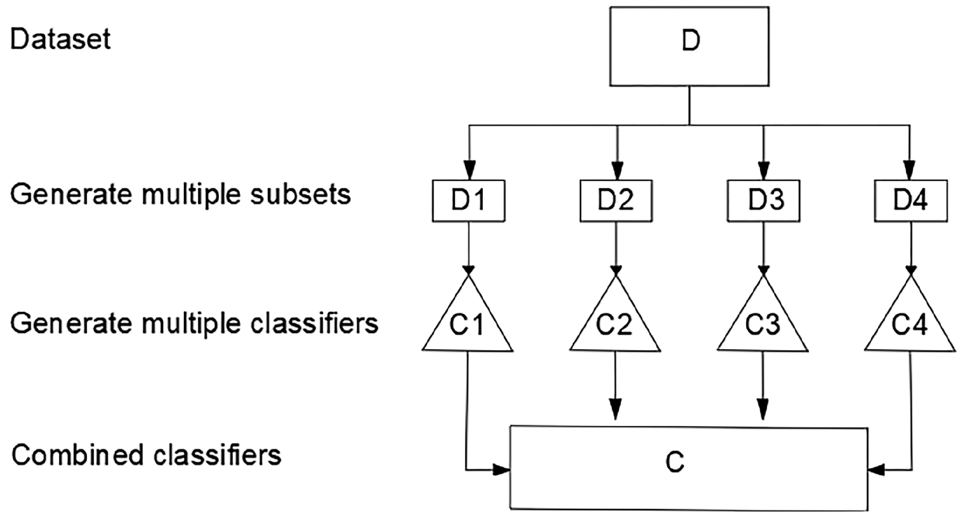
Since the gamut of hypotheses is extensive for the given data, it is difficult to maintain consistency in the accuracy of the learning algorithm and the data itself. It is also possible that the selected hypothesis may not apply to the unseen data. Additionally, the inability of the chosen scheme to find the best hypothesis may lead to error during the calculation process. The poor approximation of the target classes by the hypothesis space also poses a challenge to delineating the model. Therefore, to tackle the statistical, computational, and representation problem of the single model, ensemble learning was introduced [26]. The basic structure of ensemble learning is shown in Figure 1.

This learning algorithm involves the combination of multiple simple models (which can be called weak learners as small decision trees) to create a robust and smart model. Training of these weak learners can either be carried out through bagging (Bootstrap Aggregation) or boosting (coordinated construction of ensembles). Bagging combines these single models trained separately, whereas boosting builds models in a sequential manner and at each step, the error of the previous classifier is rectified. RF is one of the examples of the bagging algorithm; however, it also has different variants, but these are beyond the scope of this study. Despite being easy to interpret, sometimes the RF model is unable to interpret complex datasets. Therefore, there is a need for a new approach which can carry out the same task with greater efficiency and speed, without compromising the performance of the model. The variant of gradient boosting, eXtreme gradient boosting (XG Boost), was used in this study to predict the thermogravimetric behavior of pine waste.

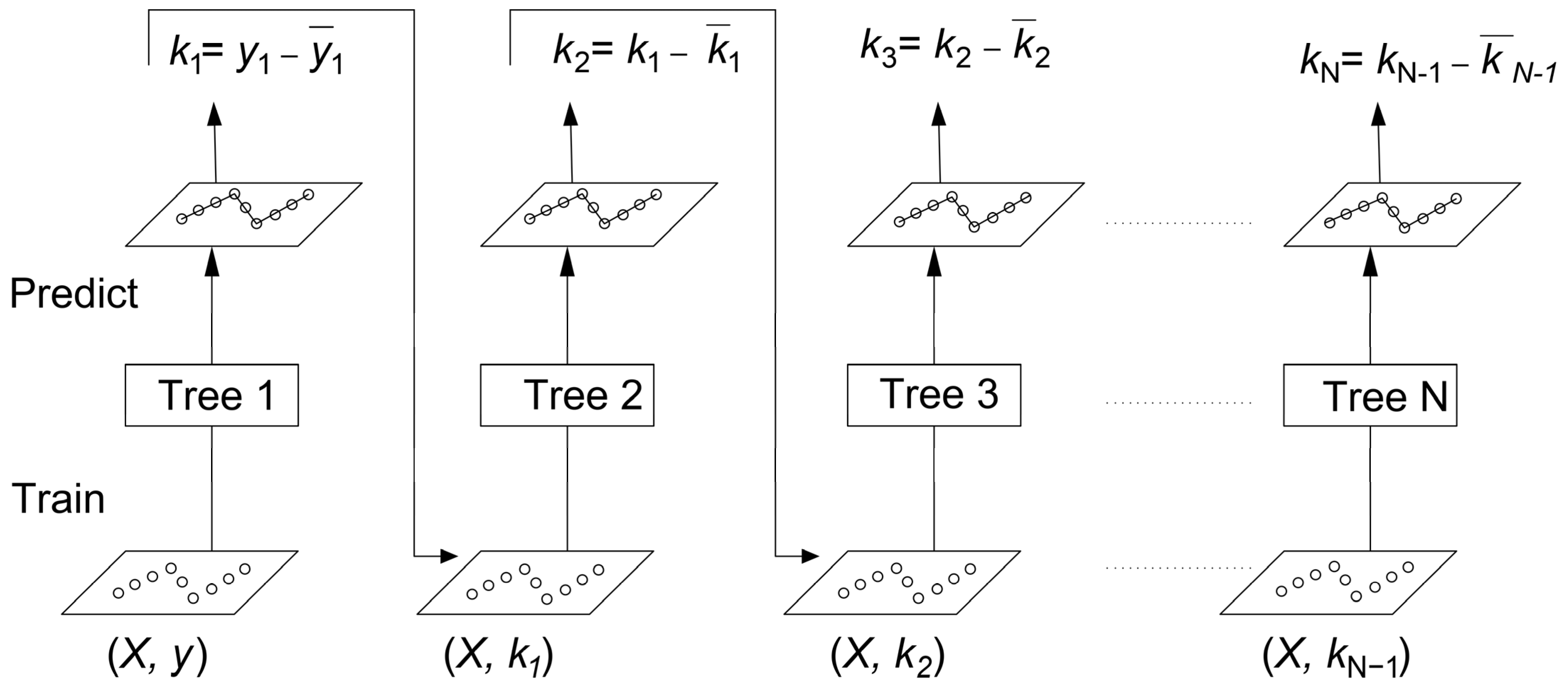
The basis of the gradient boosting (GB) algorithm relies on the same principle as in bagging. The weak learners or small trees are combined into a strong learner, where each new model in the series is trained to minimize the loss function (mean square error or cross-entropy) of the previous model with the assistance of gradient descent. In every step, the algorithm estimates the gradient of the loss function in terms of the predicted value of the current ensemble, and thereafter, it trains a new weak model to minimize the computed gradient. The predicted values of the resultant model are appended to the ensemble, and the same process is successively carried on unless a stopping condition is reached. To understand the gradient boosting, a regression example is shown in Figure 2. Here, X and y are the feature matrix and output label, respectively, which are being trained by Tree 1; k₁, k₂, k₃, …, k_N−1 denote the residual errors in each step. Correspondingly, $\overline{k}$₁, $\overline{k}$₂, $\overline{k}$₃, …, $\overline{k}$_N−1 represent the predicted values obtained as a result of each weak learner. There is another parameter that is called shrinkage or learning rate, which refers to a reduction in the prediction value obtained from each tree.

Mathematically, it can be represented by Equation (1).

$$\overline{y}=y_1+\mu k_1+\mu k_2+\dots +\mu k_N$$

(1)

Here, μ represents shrinkage, whose values vary from 0 to 1.

Unlike gradient boosting, XG Boost introduces an additional element, regularization, in the objective function, which refines its generalization and circumvents the overfitting of the model. Mathematically, the model can be given by Equation (2). Here, the initialization of the algorithm begins with the zero value of the predictor. Thereafter, each tree attempts to minimize the error associated with the weak learner.

$$\overline{y_m}={\sum }_{n=1}^N{h}_n(x_m)$$

(2)

Here, m denotes the data point, N is the number of trees in the ensemble, and the function, h_n$\left(x_m\right)$, represents the prediction value at the mth point. The next step is to formulate the objective function, which is the summation of a loss function (l) and a regularization term (ω). Equation (3) represents the objective function that is to be calculated for any given problem.

$$J={\sum }_{n=1}^{N-1}l (y_m,\overline{y_m})+{\sum }_{n=1}^N\omega \left(h_n\right)$$

(3)

The term loss function estimates the residual error between the true ($y_m$) and predicted value ($\overline{y_m}$), whereas the simplification of the tree structure is sorted by the regularization function, ω.

Rather than fitting the model straight away, the XG Boost scheme attempts to optimize the model iteratively. The initial prediction was kept $\overline{y_m}$ = $0$, and at each iteration, a new tree was added to condition the model. For an arbitrary tree count, n, the value of prediction could be represented by Equation (4).

$${\overline{y_i}}^n={\overline{y_i}}^{n-1}+h_n(x_i)$$

(4)

Another consignment is to define the regularization function, ω, which imposes a penalty on the number of leaves in a tree and the size of the leaf. It can be mathematically written as

$$\omega \left(h_N\right)=\sigma G+0.5 \phi {\sum }_{m=1}^G{\tau }_m^2$$

(5)

Here, G denotes the number of leaves in a tree, σ is a regulation factor that monitors the tree activity, and $\phi$ represents a parameter that penalizes the squared weight of the leaves, τ_m.

Another aspect of the scheme is to manage several nodes. Whether the scion is beneficial or not, or how to create a scion at each node, is decided through the information gain. The information gain at each scion can be estimated by Equation (6).

$$U=0.5 \left[{\displaystyle \frac{G_L^2}{H_L+\phi }}+{\displaystyle \frac{G_R^2}{H_R+\phi }}-{\displaystyle \frac{{\left(G_L+G_R\right)}^2}{H_L+H_R+\phi }}\right]-\sigma$$

(6)

Here, G_L and G_R represent the sums of gradients in the left and right children of the nodes, respectively. Similarly, H_L and H_R are, correspondingly, the sums of Hessians at the left and right child of the nodes. The value of information gain (U) is used by the XG Boost to identify the feature that provides the largest gain so that it can mitigate the error and enhance the performance of the model.

The benefits of the XG Boost are to reduce the complexity of trees, improve the scalability of the model as it can handle a dataset with higher dimensions, to identify the best splits, and to approximate the greedy algorithms through weighted quantiles, which is not seen in the RF. But at the same time, it is intensive, due to the likelihood of overfitting for the small datasets, and it is sensitive owing to the presence of outliers in a dataset. For the given problem, the split percentages for the training set, testing, and validation sets of the proposed TG model were 70%, 15%, and 15% of the total dataset, respectively. The loss function used for data analysis was based on regression squared error.

2.2. Thermogravimetry of Loose Biomass

For the purposes of application and training the dataset, the raw pine cones collected from the Pest region of Hungary were considered. With the help of a modified digital muffle furnace, the milled form of the pine cone was thermally processed at 250 °C for 15 min. in the fuel testing laboratory of the Department of Agriculture Machinery, in the National Agriculture and Innovation Centre, Godollo, Hungary. For the same purpose, 1.5 mm sieve was used. Thereafter, the thermogravimetric (TG) experiments (EXSTAR, Seiko Instruments Inc., Chiba, Japan) were conducted on the collected raw as well as processed samples at the Indian Instrumentation Centre, Roorkee, Uttarakhand [27]. Around 10 mg of each material underwent thermal degradation in the presence of a nitrogen atmosphere at the linear ramp rate of 5, 10, and 15 °C-min⁻¹ for the temperature range of 305–876 K. The scavenging rate of nitrogen was preset to 200 mL-min⁻¹. To measure the temperature inside the chamber, the R-type (Platinum-13% Rhodium, New York, NY, USA) thermocouple was used. The horizontal mechanism was used to avoid the buoyancy effect with the increase in the temperature of the chamber. The reason for the buoyancy is the lack of symmetry in the weighing system. It also depends on the state properties (temperature, pressure) and the nature of the gas. Therefore, the horizontal mechanism is always aiming to minimize the gas volume. It can also be sorted using empirical correction by heating an inert sample under the same thermal conditions as would have been performed on the sample of interest [28]. The ultimate analysis of raw pine cone (RPC) and processed pine cone (PPC) is conducted based on ASTM D5373 standard [29]. The physical and chemical parameters related to RPC and PPC are tabulated in

Table 1. The physical and chemical parameters related to the datasets.

Material	C%	H%	N%	O%	S%	A% 1	FC% 2	VM% 3	HHV 4	Material Density
RPC	50.40	6.77	0.65	40.83	0.10	1.22	18.43	80.35	22.10 MJ-kg−1	505 kg-m−3
PPC	55.48	5.49	0.39	34.53	0.09	4.02	82.16	13.82	28.55 MJ-kg−1	-

¹ Ash content, ² Fixed carbon, ³ Volatile matter, ⁴ Higher heating value.

. The estimated value of the bulk density of the pine cone was 672 kg-m⁻³. As a reference material, Alumina powder was used. It is to be noted that each experiment was conducted thrice.

2.3. Model-Free Technique

The estimation of kinetic parameters for the pyrolysis of pine cones was based on a model-free approach. However, it also includes the isoconversional methods, which do not require any phenomenological models for fitting purposes. To implement this methodology, it is assumed that at a given extent of reaction, the same reactions happen in the same ratio and are independent of temperature. However, this is not always true and it is possible to construct a reaction pathway that does not comply with the isoconversional approach; for example, the number of parallel independent reactions having different reactivity as a function of temperature owing to different activation energies [30] or the competitive reactions having different activation energies, which alter the reaction pathway at different temperatures [31]. Despite all these facts, this methodology is recommended by the International Confederation for Thermal Analysis and Calorimetry (ICTAC) for the kinetic analysis [32]. Here, both differential-based (Friedman) [33] as well as integral-based (Ozawa–Flynn–Wall (OFW)) [34,35] schemes were involved along with the ASTM E 698 method, Kissinger’s method, which relies on the peak reaction rate as a function of ramping rate to estimate the activation and pre-exponential factor. Kissinger’s method is, however, not in the category of isoconversional schemes [36]. This method was claimed to be an excellent approximation for first-order reactions, nth-order, nucleation-growth, and distributed reactivity model [37,38] whereas there are some cases it fails [32].

Mathematically, the model-free methodology can be deduced from the solid-state rate equation.

The rate law in the form of a single order differential in terms of product appearance, and its dependence on conversion, α, temperature, T, and pressure, P, can be written as

$$\beta {\displaystyle \frac{d\alpha }{dT}}=k\left(T\right)·j\left(p\right)·f(\alpha )$$

(7)

where k(T) represents the rate constant, and f(α) denotes the conversion function, which can be represented by Equations (8) and (9). β is the linear ramp rate for the given problem.

$$k\left(T\right)=A·e^{{\displaystyle \frac{E_a}{RT}}}$$

(8)

where A, R, and E_a are the pre-exponential function, universal gas constant, and the apparent activation energy for a given reaction, respectively.

$${\displaystyle \frac{dg\left(\alpha \right)}{d\alpha }}=f\left(\alpha \right)$$

(9)

where $g\left(\alpha \right)$ is the integral form of the solid-state reactions.

The pressure-dependent function, $j\left(p\right)$, can be expressed as

$$j\left(p\right)=\left(1-{\displaystyle \frac{P}{P_{eq}}}\right)$$

(10)

Here, P and P_eq are the partial pressure of gaseous product and the equilibrium vapor pressure, respectively.

However, the relevance of the pressure dependence is for a gas–solid reaction since the reaction rate predominantly relies on the gaseous reactant partial pressure. The characteristic of the pressure function can be either a power law or an adsorption isotherm [39]. In case of hydrocarbon cracking, this term cannot be omitted as a small perturbation in pressure would lead to a proportionate change in initiation, propagation, and termination reactions, which would ultimately cause variation in the global activation energy [40].

Friedman did not consider the pressure dependence; therefore, Equation (7) can be written as

$${\beta }_i{\displaystyle \frac{d\alpha }{dT}}=A·e^{-{\displaystyle \frac{E_{\alpha }}{R{T}_{\alpha , i}}}} f(\alpha )$$

(11)

Take the natural logarithm of Equation (9) to obtain the required expression of the Friedman method.

$$\mathit{ln}\left({\displaystyle \frac{1}{{\beta }_i}}{\displaystyle \frac{d\alpha }{dT}}\right)=\ln A-{\displaystyle \frac{E_{\alpha }}{R{T}_{\alpha , i}}}+\ln f\left(\alpha \right)$$

(12)

Similarly, the OFW method can be deduced using Doyle’s approximation for the temperature integral [41].

$$ln \left({\beta }_i\right)= ln\left({\displaystyle \frac{A_{\alpha }R}{E_{\alpha }g\left(\alpha \right)}}\right)-5.331-1.052{\displaystyle \frac{E_{\alpha }}{R{T}_{\alpha , i}}}$$

(13)

However, a more accurate version of the temperature integral was proposed by Kissinger–Akahira–Sunose (KAS), which can be expressed by Equation (12) [42].

$$\ln \left({\displaystyle \frac{{\beta }_i}{T_{\alpha ,i}^2}}\right) =ln\left({\displaystyle \frac{A_{\alpha }R}{E_{\alpha }g\left(\alpha \right)}}\right)-{\displaystyle \frac{E_{\alpha }}{R{T}_{\alpha , i}}}$$

(14)

Kissinger’s method can be derived by differentiating Equation (9) [43]. For the maximum reaction rate, put ${\displaystyle \frac{d^2\alpha }{d{T}^2}}=0$,

$$0=\left[{\displaystyle \frac{\beta E}{R{T}_{max}^2}}+A·e^{-{\displaystyle \frac{E}{R{T}_{max}}}}·{\displaystyle \frac{df\left(\alpha \right)}{d\alpha }}\right]$$

(15)

For the first-order reaction, Equation (12) can be rewritten as

$$\ln \left({\displaystyle \frac{\beta }{T_{max}^2}}\right)={\displaystyle \frac{-E_a}{R{T}_{max}}}+ln\left({\displaystyle \frac{AR}{E}}\right)$$

(16)

So, Equations (9), (11), (12), and (14) are used to estimate the kinetic parameters for RPC and PPC.

The isoconversional methods are a relatively good approach to identifying the possibility of reaction heterogeneity, which means the variety of products may be generated at different steps of the global conversion. Moreover, they are good at estimating the global conversion of a starting material as compared to model-fitting schemes, since they can easily correlate the conversion of material with both A and E. But at the same time, if someone wishes to model for intermediate product formation, they are not a good choice since the combination of generation and consumption reactions makes the reaction network too complex to estimate conversion. Additionally, the isoconversional kinetics cannot be the same for a material having an overlapped heat evolution profile.

3. Results and Discussions

This section is based on the kinetic analysis and validation of the proposed model with the experimental solution. The replicated dataset was employed to estimate the kinetic parameters for the RPC and PPC, and to determine the applicability of ML in the context of the thermal decomposition of biomass.

3.1. Thermogravimetric Analysis

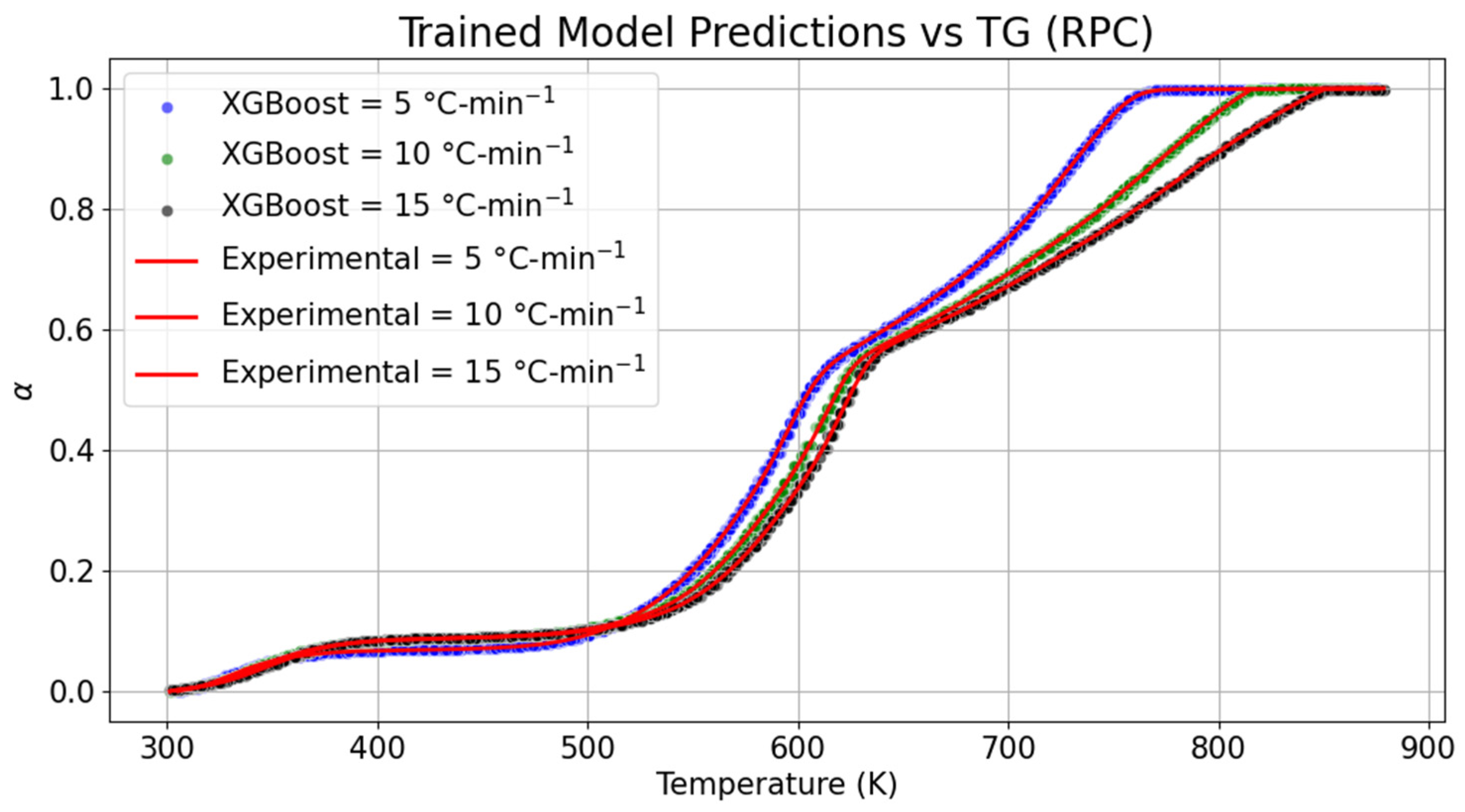
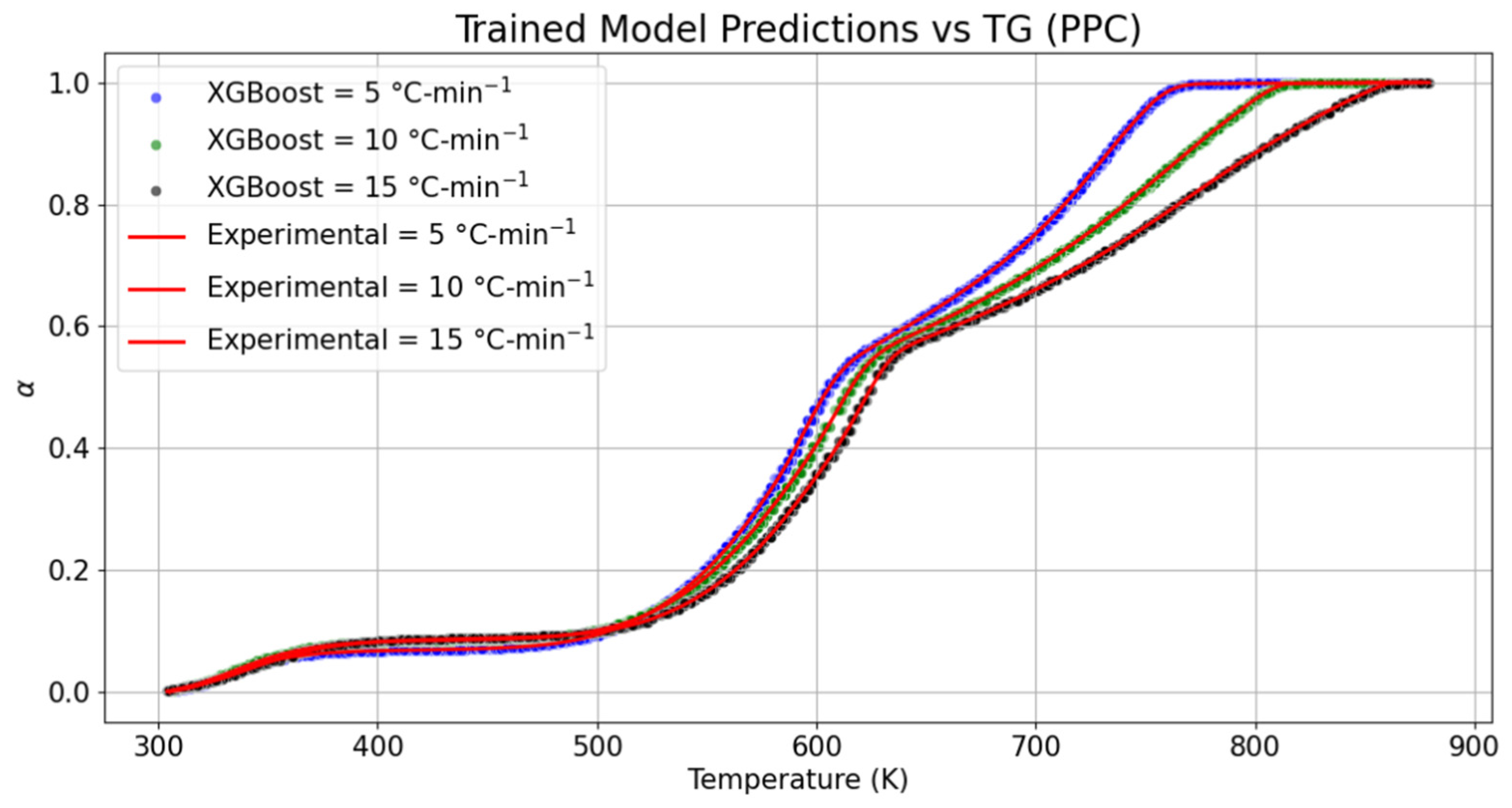
Thermogravimetric (TG) changes in the samples of RPC and PPC are shown in Figure 3 and Figure 4, respectively. The datasets of the TG curve of the RPC were trained through the extreme gradient boosting technique to implement the replicated model to derive the kinetic parameters.

Based on the comparison between the trained model and the TG graph, it was noticed that the drying stage of RPC began in the temperature range of 305–355 K with the conversion percentage of 5.38% at 5 °C-min⁻¹. In the trained model, the same conversion at the same heating rate was obtained with a marginal rise in the upper temperature range by 0.28%. As the heating rate is increased to 10 °C-min⁻¹ and 15 °C-min⁻¹, the upper limit of temperature required for drying RPC was increased by 2.19% and 3.80%, respectively. Concomitantly, the trained model was compared for the same conversion, and drops in the upper threshold of the temperature scale were 0.08% and 0.18% at 10 °C-min⁻¹ and 15 °C-min⁻¹, respectively. It can be concluded based on the distinction between the temperature range of the experimental and trained model TG curves that there is a negligible shrinkage in the evaporation boundary when examined by the ensemble learning method for RPC. Similarly, variation in devolatilization and char formation was also compared with the proposed model. As compared to the experimental datasets obtained at 5, 10, and 15 °C-min⁻¹ for RPC, it was seen that the devolatization boundaries were, respectively, dilated by 0.15 to 0.34%, 0.03 to 0.21%, and 0 to 0.09% at 5, 10, and 15 °C-min⁻¹. No drastic variation in devolatization was also seen between the trained and experimental datasets of RPC. Furthermore, temperature variation while training data during the char formation stage was relatively shrunk by 0.15% at 5 °C-min⁻¹, whereas the temperature range was increased by 5.35% and 5.86% at 10 °C-min⁻¹ and 15 °C-min⁻¹. Overall, the maximum deviation in temperature range was seen at the end of the pyrolysis of the RPC. The model performance details are provided in

Table 2. The performance metrics obtained for the proposed model.

Model	β (°C-min−1)	RMSE	MSE	MAE	R2
TG (RPC)	5	±1.85 × 10−3	3.44 × 10−6	1.12 × 10−3	0.99
	10	±1.81 × 10−3	3.30 × 10−6	1.19 × 10−3	0.99
	15	±1.83 × 10−3	3.36 × 10−6	1.34 × 10−3	0.99
DTG (RPC)	5	±6.24 × 10−4 mg-K−1	3.89 × 10−7 mg-K−1	3.13 × 10−4 mg-K−1	0.99
	10	±4.76 × 10−4 mg-K−1	2.27 × 10−7 mg-K−1	2.45 × 10−4 mg-K−1	1
	15	±5.51 × 10−4 mg-K−1	3.04 × 10−7 mg-K−1	2.56 × 10−4 mg-K−1	0.99
TG (PPC)	5	±1.83 × 10−3	3.37 × 10−6	1.13 × 10−3	0.99
	10	±1.78 × 10−3	3.20 × 10−6	1.19 × 10−3	0.99
	15	±1.82 × 10−3	3.32 × 10−6	1.36 × 10−3	0.99
DTG (PPC)	5	±4.89 × 10−4 mg-K−1	2.39 × 10−7 mg-K−1	2.97 × 10−4 mg-K−1	0.99
	10	±4.13 × 10−4 mg-K−1	1.71 × 10−7 mg-K−1	2.43 × 10−4 mg-K−1	0.99
	15	±4.98 × 10−4 mg-K−1	2.48 × 10−7 mg-K−1	2.41 × 10−4 mg-K−1	0.99
KAS	RPC	±0.48 kJ-mol−1	0.24 kJ-mol−1	4.05 kJ-mol−1	0.99
	PPC	±0.34 kJ-mol−1	0.58 kJ-mol−1	−5.67 kJ-mol−1	0.99
OFW	RPC	±0.48 kJ-mol−1	0.24 kJ-mol−1	4.88 kJ-mol−1	0.99
	PPC	±0.58 kJ-mol−1	0.34 kJ-mol−1	−7.18 kJ-mol−1	0.99
Friedman	RPC	±0.19 kJ-mol−1	0.03 kJ-mol−1	−42.99 kJ-mol−1	0.99
	PPC	±0.28 kJ-mol−1	0.08 kJ-mol−1	−68.81 kJ-mol−1	0.99
Kissinger	RPC	±9.20 × 10−2 kJ-mol−1	8.46 × 10−3 kJ-mol−1	12.89 kJ-mol−1	0.98
	PPC	±7.32 × 10−2 kJ-mol−1	5.35 × 10−3 kJ-mol−1	−7.14 kJ-mol−1	0.98

. Based on the estimated performance metrics, the root mean squared error (RMSE) obtained after the validation set varied from ±1.81 × 10⁻³ to ±1.85 × 10⁻³, whereas the coefficient of regression (R²) obtained after curve fitting was 0.99. In the same manner, the mean squared error and the mean absolute error between the predicted and true values, correspondingly, varied from 3.30 × 10⁻⁶ to 3.44 × 10⁻⁶ and 1.12 × 10⁻³ to 1.34 × 10⁻³.

For further investigation, the trained model was also compared with the TG datasets of PPC. The drying state of PPC was seen to fall in the range of 305.4–357.3 K with 5.54% conversion of the sample mass at 5 °C-min⁻¹, whereas at the same conversion percentage and heating rate, the upper threshold of temperature required for drying was marginally shrunk by 0.55%. As compared to the experimental datasets obtained at 10 °C-min⁻¹ and 15 °C-min⁻¹ with the trained model, it was noticed that the duration of drying was relatively shrunk by 1.03% for the trained model obtained at 10 °C-min⁻¹. However, the temperature range required for drying was marginally elongated by 0.20% at 15 °C-min⁻¹. In case of a change in the mass of samples of PPC during release of volatile gases, the duration of devolatilization captured through the trained model was slightly extended by 0.42% at 5, 0.14% at 10 °C-min⁻¹, and 0.02% at 15 °C-min⁻¹. The behavior of the trained model during the charring process, as compared to the experimental datasets, depicted that the temperature scale required for char formation at 5, 10, and 15 °C-min⁻¹ was, respectively, diminished by 0.02%, 0.26%, and 0.07%. It is clear from both the materials that there is a marginal drift in the thermogravimetric boundaries predicted by the proposed model, irrespective of the heating rates and material. The RMSE values obtained at 5, 10, and 15 °C-min⁻¹ for the trained TG models of PPC were, respectively, ±1.83 × 10⁻³, ±1.78 × 10⁻³, and ±1.82 × 10⁻³. In the same manner, MSE was noticed to be constant for all predicted models obtained at different heating rates. The variation in MAE encountered during the validation of TG models was in the range of 1.13 × 10⁻³–1.36 × 10⁻³.

Statistically, based on t-statistics and p-value, no significant statistical difference between the model and the experimental datasets of both RPC and PPC was observed. Distribution functions obtained at different heating rates were positively skewed for both trained and experimental datasets of RPC and PPC. However, the marginal quantitative deviation in their values was encountered with the rising heating rate. The kurtosis in the distribution function of conversion, α, was relatively high in the trained models (super-Gaussian characteristic) obtained at a higher heating rate. In other words, as compared to the experimental datasets, the variability in the predicted datasets increased with the increasing heating rates.

3.2. Derivative Thermogravimetric Analysis (DTG)

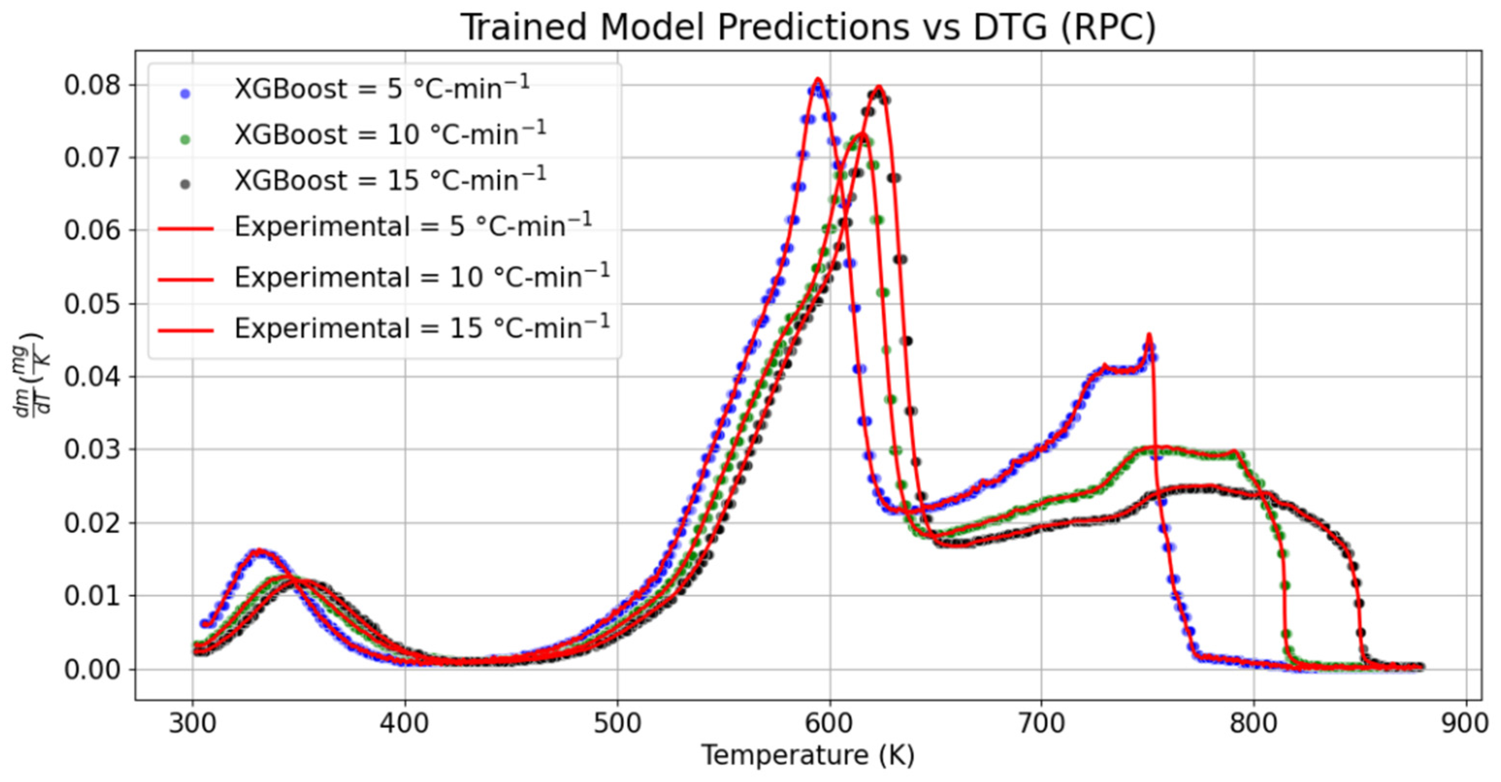
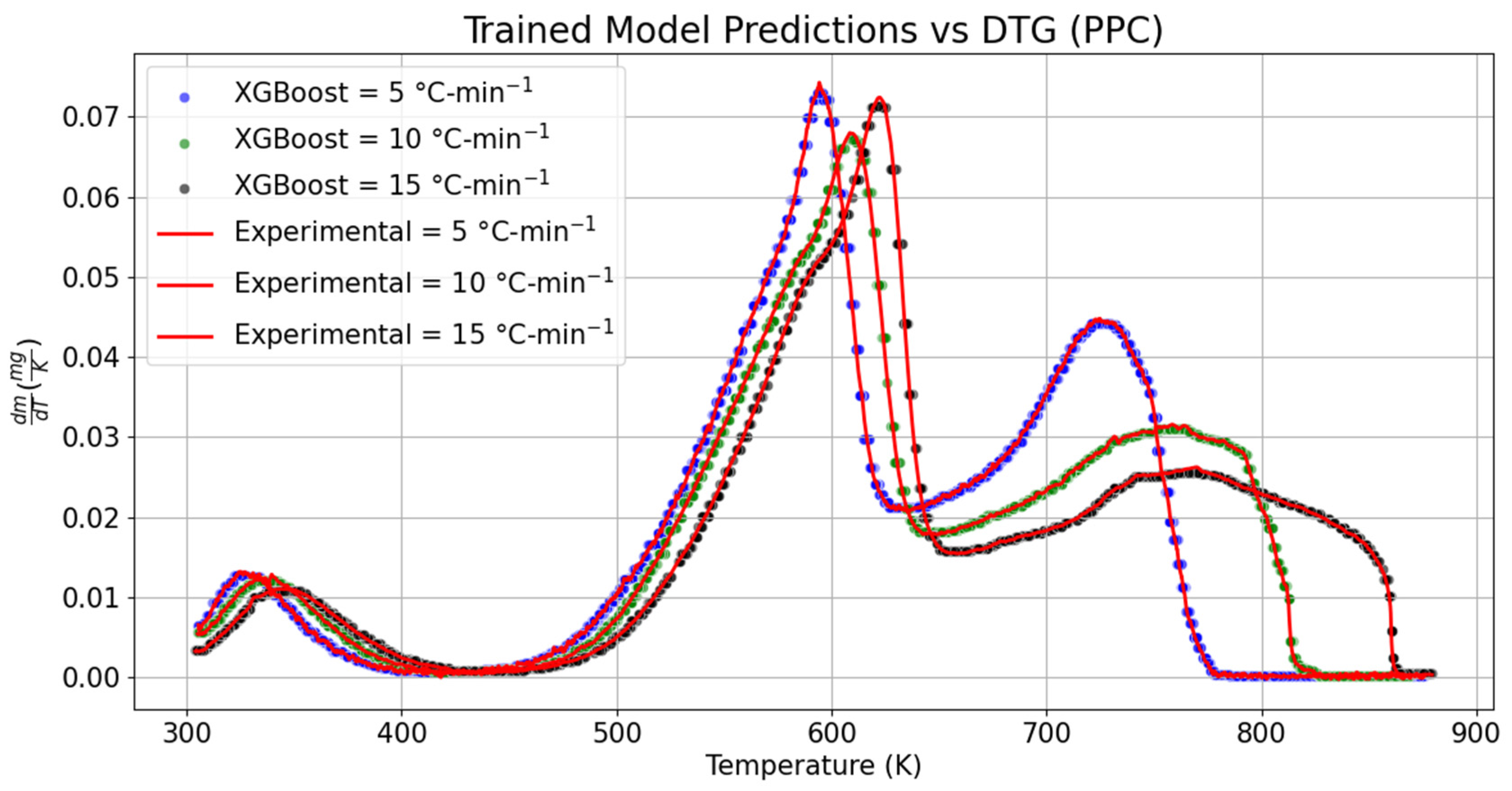
The variation in the sample mass over the given temperature range for RPC and PPC is, respectively, shown in Figure 5 and Figure 6. To compare the global/local maximum and the decomposition of cellulose, hemicellulose, and lignin, the trained model was validated with the 15% DTG datasets of RPC and PPC. The range of temperature over which hemicellulose decomposition was noticed to happen was 303.1 to 426.1 K, with a rate of change in mass of 2.76% per second (0.05% per K) at 5 °C-min⁻¹, which was approximately 37.50% lower than the recorded value for the predicted dataset at the same heating rate. The change in mass with temperature over the plateau of 408–416.50 K was seen to be fairly constant, which was not perceived in the experimental DTG of RPC. The temperature range of hemicellulose decomposition shrunk by 2.11%. In the same manner, the position of the local maximum (hemicellulose peak) was relatively shifted towards the left by the narrow margin of 0.03%, whereas the change in mass at the same position was also diminished by 0.99% for the predicted DTG model of RPC at 5 °C-min⁻¹. Similarly, as compared to the experimental DTG curves, the local maxima obtained from the predicted DTG models at 10 °C-min⁻¹ and 15 °C-min⁻¹ also dropped by 1.35% and 1.83%, respectively. As compared to the experimental DTG datasets, the temperature range over which hemicellulose decomposed at 10 °C-min⁻¹ was relatively dilated by 0.54% in the predicted DTG model. However, it was not seen while modeling the DTG graph at 15 °C-min⁻¹ and the hemicellulose decomposition zone was shrunk by 0.67%. Comparatively, relative jumps of 13.49% and 18.03% were, correspondingly, seen in the change in mass of RPC at the end of hemicellulose decomposition predicted by the trained DTG models at 10 °C-min⁻¹ and 15 °C-min⁻¹. Likewise, the magnitude of global maxima obtained from the trained models at 5, 10, and 15 °C-min⁻¹ dropped by 0.95%, 0.69%, and 0.90%, respectively.

The location of the global maximum in the trained model was also relatively shifted towards the right (or there was a delay in reaching the cellulose decomposition) by 0.3 K at 5 °C-min⁻¹, 0.2 K at 10 °C-min⁻¹, and 0.5 K at 15 °C-min⁻¹. Relatively, as compared to the experimental values, the prediction of the slow decomposition rate of the lignin model over the wide range of temperature was noticed to have a positive drift in its temperature range by 1.2 K at 5 °C-min⁻¹, whereas a negative shift of 0.17% and 0.05% was seen, respectively, at 15 °C-min⁻¹ in the temperature scale for the lignin decomposition. The change in mass with temperature was relatively lowered by 1.55% at 5 °C-min⁻¹. With the increasing heating rate, it was reduced by 0.52% at 10 °C-min⁻¹. Conversely, a negotiable increase of 0.02% was recorded in the proposed DTG model at 15 °C-min⁻¹. Seeing the performance metrics, the RMSE values varied from ±4.13 × 10⁻⁴ mg-K⁻¹ to ±4.98 × 10⁻⁴ mg-K⁻¹ for the proposed DTG models. Similarly, the MSE values were, respectively, 2.39 × 10⁻⁷ mg-K⁻¹, 1.71 × 10⁻⁷ mg-K⁻¹, and 2.48 × 10⁻⁷ mg-K⁻¹ at 5, 10, and 15 °C-min⁻¹. The estimated values of the MAE obtained for the trained models were in the range of 2.41 × 10⁻⁴ mg-K⁻¹ to 2.97 × 10⁻⁴ mg-K⁻¹. Based on the established relationship, it can be concluded that a marginal deviation was seen in the decomposition peaks of cellulose, hemicellulose, and lignin. A shift in temperature scale with the increasing heating rate was reasonably captured by the trained DTG models of RPC. A similar overlapping peak pattern was also noticed while examining the DSC dataset with the machine learning technique [42].

In the same pursuit, the DTG datasets of PPC were also examined to determine whether features of the datasets were captured by the predicted DTG models or not. While comparing the results with experimental datasets, it was seen that the local maximum was relatively shifted by 0.12% towards the left with an increase in the decomposition rate by 1.15%. The temperature scale over which the hemicellulose decomposition took place was also shrunk by 1.08% for the trained DTG model of PPC at 5 °C-min⁻¹. Similarly, the temperature range required for cellulose decomposition was also shortened by 0.34%, whereas it was relatively dilated by 0.14% while predicting the slow decomposition rate of lignin content at 5 °C-min⁻¹. No shift in the location of the global maximum was seen; however, the maximum decomposition rate of PPC dropped by 1.60% for the trained DTG model at 5 °C-min⁻¹. The temperature scale required for the decomposition of lignin was diminished by 0.03% while comparing the trained DTG model with the experimental DTG at 5 °C-min⁻¹. The corresponding value obtained from the trained DTG model at 5 °C-min⁻¹ underpredicted the lignin decomposition by 0.56%.

The change in the decomposition rate for hemicellulose, cellulose, and lignin was compared with the experimental DTG dataset at 10 °C-min⁻¹. It was noticed that the range of hemicellulose decomposition shifted by 2.13% towards the right, whereas the positive drift in the local maximum position was 0.17%. The maximum rate of change in mass with temperature at the local maximum dropped by 2.97%. In the same manner, the cellulose peak was shifted towards the right by 0.09%. The predicted change in mass during cellulose decomposition was reduced by 0.63% at the peak point. The range of temperature required for the cellulose decomposition was also curtailed by 0.09% for the trained DTG model at 10 °C-min⁻¹. At the same heating rate, the temperature range required for the slow decomposition rate of lignin was relatively dilated by 0.12% when it was compared with the experimental DTG dataset. The lignin peak was also noticed to be deviated toward the right by 0.18% in the trained DTG model, whereas the location of the lignin peak was drifted by 1.4 K in the right direction. In the predicted dataset, the temperature scale required for the decomposition of lignin was marginally dilated by 0.12%.

The temperature scale required for decomposition of hemicellulose, cellulose, and lignin in the predicted datasets was, respectively, extended by 1.81%, 0.03%, and 0.02% at 15 °C-min⁻¹. Similarly, the decomposition peak position for hemicellulose was deviated by 0.60% in the left direction, whereas a positive drift of 0.16% was recorded while capturing the lignin decomposition peak at 15 °C-min⁻¹ for the predicted DTG model. The predicted model accurately predicted the global maximum position at 15 °C-min⁻¹; however, quantitatively, the change in mass of PPC with temperature was reduced by 0.80%, which was, respectively, lowered by 2.17% and 2.09% in the case of hemicellulose and lignin. The performance metric for predicted DTG models of PPC had RMSE values of ±4.89 × 10⁻⁴ mg-K⁻¹, ±4.13 × 10⁻⁴ mg-K⁻¹, and ±4.98 × 10⁻⁴ mg-K⁻¹ at 5, 10, and 15 °C-min⁻¹, respectively. Likewise, the MSE varied from 1.71 × 10⁻⁷ mg-K⁻¹ to 2.48 × 10⁻⁷ mg-K⁻¹. The maximum MAE was seen while modeling the DTG dataset at 5 °C-min⁻¹.

The results obtained through t-statistics and p-value are consistent with the obtained solution for the proposed TG models. No evidence was found to depict the statistical deviation between the trained and experimental datasets of DTG. No appreciable change was seen in the skewness of the distribution function obtained through the trained model. It can be concluded that the validation datasets of TG and DTG captured precisely the features of the experimental datasets of TG and DTG. The effect of anomalies in the trained datasets with the experimental solution was examined with the help of the isoconversional kinetic models.

3.3. Validation of the Trained Model

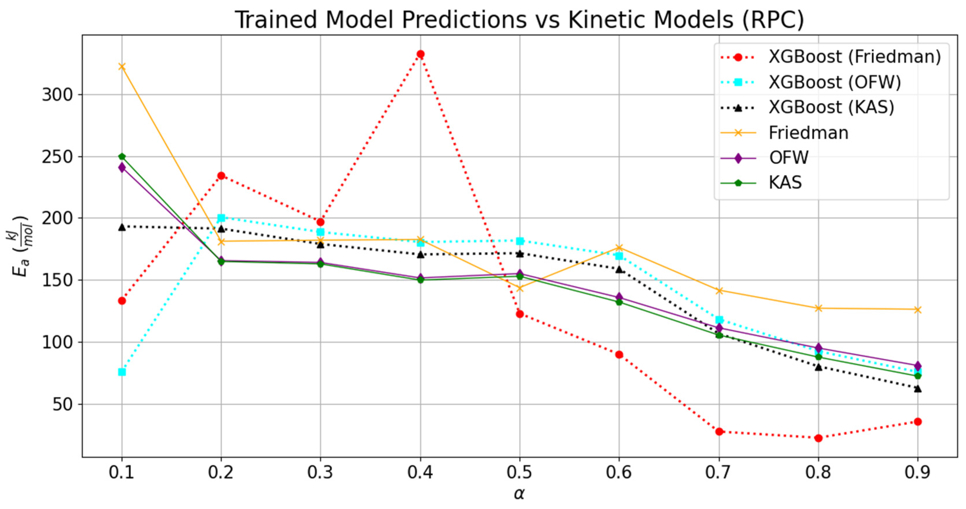
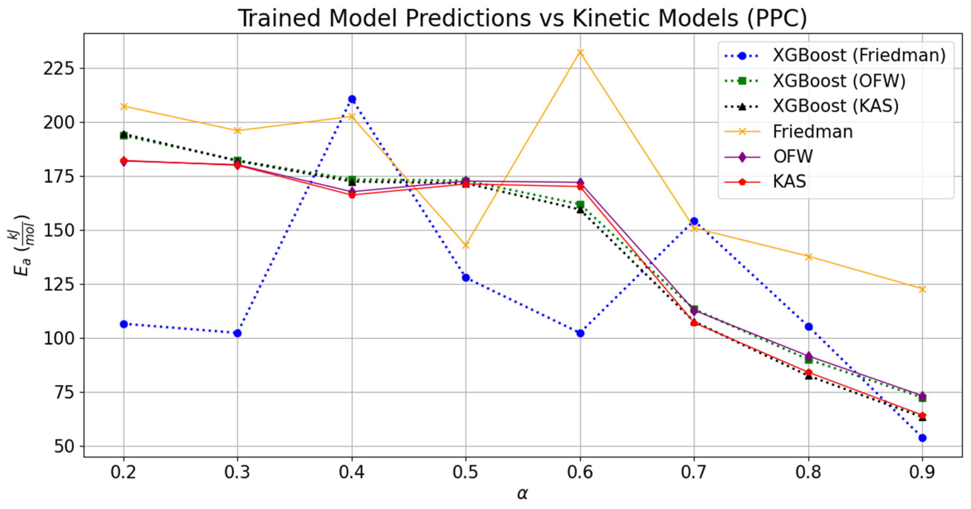
The comparisons of the validated models with the experimentally derived values are shown in Figure 7 and Figure 8. The replicated models for TG and DTG were tested to estimate the kinetic parameters associated with the thermal decomposition of RPC and PPC. The values obtained through the experimental datasets for RPC and PPC are tabulated in

Table 3. Estimated kinetic parameters for thermal degradation of RPC.

Conversion	Differential			Integral
	Friedman			OFW			KAS
α	Ea (kJ-mol−1)	A (min.−1)	R2	Ea (kJ-mol−1)	A (min.−1)	R2	Ea (kJ-mol−1)	A (min.−1)	R2
0.1	322.58	2.47 × 1036	0.97	241.10	1.01 × 1028	0.98	249.66	2.78 × 1019	0.97
0.2	181.24	5.27 × 1018	0.99	165.59	1.52 × 1017	0.99	164.94	3.18 × 108	0.99
0.3	182.07	1.23 × 1018	0.99	164.11	3.64 × 1016	0.99	162.95	6.94 × 107	0.99
0.4	182.65	4.63 × 1017	0.99	151.64	1.29 × 1015	0.99	149.90	2.30 × 106	0.99
0.5	143.83	1.34 × 1014	1	155.13	1.60 × 1015	0.99	152.97	2.72 × 106	0.99
0.6	176.25	6.82 × 1016	0.95	135.85	8.83 × 1012	0.95	132.19	1.35 × 104	0.94
0.7	141.83	1.95 × 1013	0.98	111.40	1.99 × 1010	0.99	105.58	25.54	0.98
0.8	127.20	5.29 × 1011	0.98	95.11	4.11 × 108	0.99	87.79	0.45	0.99
0.9	126.37	2.65 ×1011	0.99	80.99	2.44 × 107	0.99	72.43	0.02	0.99
Average	176	2.75 × 1035	-	144.54	1.19 × 1027	-	142.04	3.09 × 1018	-
Kissinger	103.67 kJ-mol−1	2.20 × 108	0.98

and

Table 4. Computed kinetic parameters related to the PPC.

Conversion	Differential			Integral
	Friedman			OFW			KAS
α	Ea (kJ-mol−1)	A (min.−1)	R2	Ea (kJ-mol−1)	A (min.−1)	R2	Ea (kJ-mol−1)	A (min.−1)	R2
0.1	335.46	1.74 × 1039	1	211.63	1.17 × 1030	1	214.33	3.04 × 1020	1
0.2	207.43	3.90 × 1022	0.83	182.00	9.91 × 1024	0.84	182.24	2.04 × 1015	0.83
0.3	196.04	2.22 × 1020	0.91	180.26	1.79 × 1024	0.92	180	3.39× 1014	0.91
0.4	202.61	1.25 × 1020	0.94	167.77	4.88 × 1022	0.96	166.24	8.56 × 1012	0.96
0.5	143.00	3.03 × 1014	0.97	172.68	7.38 × 1022	0.98	171.35	1.23 × 1013	0.96
0.6	232.45	2.27 × 1021	0.97	172.11	1.19 × 1022	0.97	170.18	1.77 × 1012	0.98
0.7	150.98	5.42 × 1013	0.98	112.92	2.25 × 1016	0.98	107.16	2.77 × 106	0.97
0.8	137.92	9.93 × 1011	0.98	91.74	2.34 × 1014	0.99	84.22	2.52 × 104	0.98
0.9	122.88	2.69 × 1010	0.99	73.35	6.75 × 1012	0.99	64.37	640	0.98
Average	192	1.94 × 1038		151.61	1.30 × 1029		148.89	3.37 × 1019	0.98
Kissinger	110.65 kJ-mol−1	1.033 × 109	0.98

, respectively. Similarly, the parameters retrieved through the trained model for RPC and PPC are, respectively, provided in

Table 5. The kinetic parameters obtained through the trained kinetic model for RPC.

Conversion	Differential			Integral
	Friedman			OFW			KAS
α	Ea (kJ-mol−1)	A (min.−1)	R2	Ea (kJ-mol−1)	A (min.−1)	R2	Ea (kJ-mol−1)	A (min.−1)	R2
0.1	133.55	3.57 × 1012	0.97	175.76	1.34 × 1024	0.99	193.20	1.31 × 1028	0.89
0.2	234.31	6.22 × 1021	0.37	190.69	7.36 × 1025	0.90	191.38	1.56 × 1017	0.89
0.3	197.17	3.36 × 1017	0.25	179.28	1.41 × 1024	0.93	179.00	2.73 × 1015	0.92
0.4	332.70	3.99 × 1029	0.47	171.65	1.05 × 1023	0.97	170.60	1.91 × 1014	0.97
0.5	123.04	1.37 × 1010	0.92	172.83	5.36 × 1022	0.96	171.60	1.23 × 1014	0.96
0.6	90.08	1.86 × 106	0.92	161.45	1.34 × 1021	0.96	158.96	2.03 × 1012	0.95
0.7	27.73	2.16 × 104	0.99	112.53	2.03 × 1016	0.99	106.75	2.56 × 107	0.98
0.8	22.73	8.59 × 103	0.99	112.21	1.46 × 1014	0.99	80.36	1.26 × 105	0.99
0.9	35.76	1.16 × 105	0.99	72.02	5.10 × 1012	0.99	62.98	6.18 × 104	0.98
Average	133.01	4.44 × 1028		149.82	8.50 × 1024		146.09	1.45 × 1027
Kissinger	116.56	3.40 × 109	0.98

and

Table 6. The kinetic parameters obtained through the trained kinetic model for PPC.

Conversion	Differential			Integral
	Friedman			OFW			KAS
α	Ea (kJ-mol−1)	A (min.−1)	R2	Ea (kJ-mol−1)	A (min.−1)	R2	Ea (kJ-mol−1)	A (min.−1)	R2
0.1	144.49	9.52 × 1012	0.86	139.33	1.03 × 1020	0.75	154.80	1.01 × 1024	0.77
0.2	106.66	2.55 × 1011	0.89	193.78	1.47 × 1026	0.88	194.54	3.14 × 1017	0.87
0.3	102.42	2.33 × 1010	0.37	182.24	2.69 × 1024	0.92	182.07	5.23 × 1015	0.91
0.4	210.92	1.07 × 1012	0.79	173.47	1.57 × 1023	0.97	172.51	2.86 × 1014	0.97
0.5	127.97	2.23 × 109	0.97	172.91	7.39 × 1022	0.96	171.68	1.26 × 1014	0.96
0.6	102.42	2.35 × 1010	0.98	162.01	1.48 × 1021	0.96	159.54	2.25 × 1012	0.95
0.7	154.39	2.65 × 103	0.98	113.4	2.40 × 1016	0.98	107.66	3.02 × 107	0.97
0.8	105.50	5.06 × 103	0.98	90.17	1.68 × 1014	0.99	82.62	1.86 × 105	0.99
0.9	54.00	1.48 × 104	0.99	72.50	5.51 × 1012	0.99	63.48	5.72 × 104	0.99
Average	123.19	9.52 × 1012		144.42	1.67 × 1025		143.21	1.13 × 1023
Kissinger	103.50	2.47 × 108	0.98

. The effect of deviation in the predicted TG and DTG datasets can be noticed through the relative variation in the regression models. As compared to the experimentally derived values of activation energies at different conversion points, the relative fitting of the temperature scale over the conversion was rather low, and it can be seen through the difference between the MAE values for different kinetic models. However, the overall regression coefficient was seen to be constant for kinetic models derived from the predicted TG and DTG datasets.

Comparatively, the replicated TG and DTG models and kinetic parameters obtained through them provided a relatively good consensus with the experimentally derived values for the KAS model, followed by the OFW and Kissinger methods. The average activation energies derived through trained datasets of RPC and PPC for KAS, OFW, and Kissinger models were, respectively, 146.09 kJ-mol⁻¹, 149.82 kJ-mol⁻¹, and 116.56 kJ-mol⁻¹, and 143.21 kJ-mol⁻¹, 144.42 kJ-mol⁻¹, and 103.50 kJ-mol⁻¹. The results obtained from integral methods (KAS and OFW) were also compared with the differential method (Friedman). Deviations of 12.63% and 9.83% in the derived activation energy values from OFW and KAS were seen with respect to the corresponding value estimated through the Friedman method for RPC. Likewise, this difference in activation energies obtained through trained models relatively soared up to 17.23% and 16.25% for PPC. Relatively, the variation in the kinetic parameters derived from the OFW model using trained datasets was 29.35% lower than that seen in the corresponding values computed from the experimental datasets for RPC. This margin further dropped by 49% while juxtaposing the deviation obtained in the activation energies from KAS and Friedman with the experimentally derived values for RPC. In the case of PPC, the relative change in the activation energies derived from integral and differential methods using experimental datasets was 21.03 to 22.45% higher than the corresponding difference seen in the activation energies derived through the trained models. It is clear from the machine learning programming that the relative deviation in the kinetic parameters fetched through the boosting technique was drastically lower than the experimental values. But it also has certain limitations related to the multiclassification in the datasets. It was seen that the kinetic parameters obtained through the Friedman method have the highest MAE as compared to the MAEs encountered in OFW, KAS, and Kissinger. The addition of several features was not seen to be beneficial in capturing the data signal. It rather provided the noisy data; therefore, it led to the drastic deviations of 42.99 kJ-mol⁻¹ and 68.81 kJ-mol⁻¹ for RPC and PPC, respectively. As compared to the activation energies derived through the Kissinger method using experimental datasets, the activation energies obtained using the trained DTG datasets for the same methodology were, respectively, deviated by 12.97 kJ-mol⁻¹ and −7.14 kJ-mol⁻¹ for RPC and PPC. The data pattern of variation in frequency factors (A) with activation energy was predicted fairly for all the kinetic models; however, the quantitative variation was relatively high as compared to the corresponding values derived from the experimental datasets. The lowest variation was seen in the Kissinger model, which estimated the kinetic parameters using the predicted trained DTG models of RPC and PPC. The relative increase or decrease in the frequency factors derived through Friedman, OFW, KAS, and Kissinger using the predicted values was, respectively, −100, −99.30, 4.69 × 10⁸, and 14.50, and −1, −1, 3350, and −0.76 for RPC and PPC. So, the maximum deviation was seen while simultaneously estimating the kinetic parameters in OFW; albeit, it was not the case when the activation energy was compared. This means the coordinated ensemble learning may not provide the best solution if the number of features is added to the XG Boost technique. The results were compared with the ANN model proposed by Yao et al. (2025), and they were in good agreement with the estimated solution [24].

Despite the good convergence for the large datasets, the objective of the chosen methodology is still unable to comprehend the underlying relationship between features and target variables, which is one of the challenging aspects of the XG Boost. Moreover, the range limitation or extrapolation issue was also noticed while using the coordinated ensemble technique. Similar kinds of issues were also deeply discussed by Chen et al. (2024) [19].

4. Conclusions

The ensemble learning technique was used to predict the TG and DTG datasets and its effect on the kinetic models was evaluated using the kinetic models. Based on the relative analysis of datasets derived for both RPC and PPC, the following conclusions were inferred.

• The predicted models for TG and DTG curves have shown marginal deviation in the temperature scale. Comparatively, the maximum variation in the proposed model was seen while predicting the TG datasets during the drying process at higher heating rates. However, the change in mass with temperature was fairly predicted, but the temperature scale was either shrunk or dilated. The prediction of the release of volatile gases through the trained model for both RPC and PPC did not show any appreciable change. However, the distribution characteristic of trained datasets relatively supported the higher-order Gaussian function. In the context of the prediction of DTG curves, the range of temperature required for hemicellulose decomposition shows the maximum change as compared to cellulose and lignin for RPC and PPC. It was noticed that the shift of 2.11% was seen in the trained model for RPC at 5 °C-min⁻¹. For both materials, the lowest RMSE value proposed was estimated at 10 °C-min⁻¹, whereas the highest value was recorded at 5 °C-min⁻¹.
• While computing the kinetic parameters using the replicated datasets, the deviation in the activation energy was at its maximum for the differential method. In case of frequency factor variation, the OFW surpassed the other methodology. A good consensus between the predicted and experimentally derived kinetic parameters was seen for the KAS method, followed by Kissinger. The underpredicted values of kinetic parameters were predominantly seen while determining the solution for PPC. A limitation is encountered if the regression model is way too simple and has multiple classifications for the chosen objective function. However, the XG Boost technique produced a robust solution for the large datasets. It can be sorted using the support vector regression or basic lasso regression technique. Based on the comparative aspect, it is relatively easy to incorporate the vast library with Python (version 3.13.2) and it can be easy to use, but the memory management of Rust could be relatively good when both are juxtaposed for the machine learning technique [43].